


Languages
Pages
Legal


WP-2013-004
Distribution fees and mutual fund flows: Evidence from a naturalexperiment in the Indian mutual funds market
Santosh Anagol, Vijaya Marisetty, Renuka Sane and Buvaneshwaran Venugopal
Indira Gandhi Institute of Development Research, MumbaiFebruary 2013
http://www.igidr.ac.in/pdf/publication/WP-2013-004.pdf

Distribution fees and mutual fund flows: Evidence from a naturalexperiment in the Indian mutual funds market
Santosh Anagol, Vijaya Marisetty, Renuka Sane and Buvaneshwaran VenugopalIndira Gandhi Institute of Development Research (IGIDR)
General Arun Kumar Vaidya Marg Goregaon (E), Mumbai- 400065, INDIA
Email (corresponding author): [email protected]
Abstract
Mutual fund companies typically charge investors distribution fees, such as 12b-1 fees in the United
States, which they then use to pay commissions to brokers. We evaluate a major Indian investor
protection reform that limited the ability of mutual funds to charge distribution fees to pay broker
commissions. We identify the impact of this policy change by comparing funds charging high
distribution fees prior to the reform to those charging low distribution fees; we show that trends in asset
growth across these groups prior to the reform were similar, and argue that a comparison of their asset
growth after the reform is indicative of the policy impact. Contrary to industry claims that banning
distribution fees would dramatically reduce investment in mutual funds, we find no evidence that the
post-reform asset growth was lower for funds charging higher distribution fees prior to the reform. We
primarily find that asset growth in funds with previously high distribution fees was higher after the
policy change. At the aggregate level, our results suggest that Indian mutual fund growth in the
post-policy period was lower for reasons independent of this policy change, such as a general move
away from mutual funds towards real assets such as gold and real estate following the 2008 financial
crisis.
Keywords: regulation, commission ban
JEL Code: JEL Codes: G23, G28
Acknowledgements:
We thank Shawn Cole, Ruchi Chojer, Mark Duggan, Fernando Ferreira, Keith Gamble, Ginger Jin, G. Sethu, Saikat Deb, Sayee
Srinivasan, K. N. Vaidyanathan, Shing-YiWang and participants atWharton, the IGIDR Emerging Markets Finance Conference,
and the 2013 American Economic Association conference for valuable feedback. We thank ACE Fintech Pvt Ltd for providing
access to the Indian mutual funds data, and Karvy Computershare Limited for access to disaggregated data on mutual fund ows.
We thank the Center for the Advanced Study of India at the University of Pennsylvania for funding. Maria Guo, Mengshu Shen,
and Jason Tian provided excellent research assistance. This paper was earlier circulated as: "Are Mutual Funds Sold or Bought?
Evidence from the Indian Mutual Funds Market".
Distribution Fees and Mutual Fund Flows: Evidence from a
Natural Experiment in the Indian Mutual Funds Market∗
Santosh Anagol1, Vijaya Marisetty2, Renuka Sane3, and Buvaneshwaran Venugopal4
1Wharton2RMIT University
3Finance Research Group, Indira Gandhi Institute for Development Research4C.T. Bauer College of Business, University of Houston
February 4, 2013
Abstract
Mutual fund companies typically charge investors distribution fees, such as 12b-1 fees inthe United States, which they then use to pay commissions to brokers. We evaluate a majorIndian investor protection reform that limited the ability of mutual funds to charge distributionfees to pay broker commissions. We identify the impact of this policy change by comparingfunds charging high distribution fees prior to the reform to those charging low distributionfees; we show that trends in asset growth across these groups prior to the reform were similar,and argue that a comparison of their asset growth after the reform is indicative of the policyimpact. Contrary to industry claims that banning distribution fees would dramatically reduceinvestment in mutual funds, we find no evidence that the post-reform asset growth was lower forfunds charging higher distribution fees prior to the reform. We primarily find that asset growthin funds with previously high distribution fees was higher after the policy change. At theaggregate level, our results suggest that Indian mutual fund growth in the post-policy periodwas lower for reasons independent of this policy change, such as a general move away frommutual funds towards real assets such as gold and real estate following the 2008 financial crisis.
∗We thank Shawn Cole, Ruchi Chojer, Mark Duggan, Fernando Ferreira, Keith Gamble, Ginger Jin, G. Sethu,Saikat Deb, Sayee Srinivasan, K. N. Vaidyanathan, Shing-Yi Wang and participants at Wharton, the IGIDR EmergingMarkets Finance Conference, and the 2013 American Economic Association conference for valuable feedback. Wethank ACE Fintech Pvt Ltd for providing access to the Indian mutual funds data, and Karvy Computershare Limitedfor access to disaggregated data on mutual fund flows. We thank the Center for the Advanced Study of India atthe University of Pennsylvania for funding. Maria Guo, Mengshu Shen, and Jason Tian provided excellent researchassistance. This paper was earlier circulated as: “Are Mutual Funds Sold or Bought? Evidence from the IndianMutual Funds Market”.
1

1 Introduction
The financial crisis of 2008 spurred an active policy debate on the optimal way to pursue consumer
financial protection (Campbell et al., 2011). Two main policy options have received attention (Ko
and Lee, 2011). One approach is to empower consumers to make better financial decisions through
financial literacy training and disclosure regulation. A small but growing literature evaluates fi-
nancial literacy training programs, with mixed results.1
Another policy approach is direct intervention into how financial products are sold, such as capping
or banning commissions to financial product brokers. A number of significant reforms have already
been made. As of January 1, 2013, The U.K. Financial Services Authority has implemented a ban
on commissions paid to independent financial advisors by financial product providers (Collinson,
2012). Australia will implement a similar ban on commissions in July 2013 (Bowen, 2011). There
is also a longstanding policy debate in the United States on whether mutual funds should be
allowed to charge a separate class of operating expenses, known as 12b-1 fees, specifically for the
purpose of paying distribution expenses such as broker commissions (Ferris and Chance (1987),
Walsh (2005)).2
Commissions bans are motivated by the idea that commissions influence brokers to sell products
that are not necessarily in line with the interest of their customers (Anagol et al. (2012), Mul-
lainathan et al. (2012)). Policymakers hope that by eliminating commissions, investors will be
more likely to directly pay for financial advice, and will become more aware about how brokers
are compensated. On the other hand, brokers and financial product companies argue that commis-
sions bans reduce the incentive for brokers to educate consumers about financial products ((Sriram,
2012), (Basu and Govindaraj, 2012)). Despite the fact that major reforms have already been un-
dertaken, we have little empirical evidence on how interventions to reduce commissions affect the
distribution of financial products.
This paper provides the first estimates of the impact of a major policy reform aimed at reducing
commissions paid to brokers to sell financial products. We exploit a policy change that occurred
on August 1, 2009, in which the Securities Exchange Board of India (SEBI) banned entry loads
charged by all mutual fund firms operating in India.3 Prior to this reform, mutual fund firms used
entry loads primarily to pay commissions to brokers who sold their products. The stated goal of the
1Carlin and Robinson (2011), Cole et al. (2011), Hastings and Mitchell (2011), Cole and Shastry (2010) presentevaluations of financial literacy programs in a variety of contexts. For a recent review of financial literacy programs,see Hastings et al. (2012).
2Walsh (2005) references a 1995 Investment Company Institute report that shows 63 percent of 12b-1 fees areused for compensation of broker-dealers and related expenses.
3An entry load, typically called a “front-end load” in the U.S., is a fee that is calculated as a percentage of thetotal investment made in the mutual fund. Entry loads are immediately deducted from the customer’s investment atthe time of investment.
2

policy was to “empower the investor in deciding the commission paid to the distributors and also
to ensure transparency in commissions paid for mutual fund products”.4 This law change reduced
the ability of mutual funds to pay broker commissions, as funds could no longer use the immediate
income earned from an investor’s entry load to pay out a commission to the broker who made the
sale.5
The ban on entry loads could have multiple potential impacts on flows into mutual funds. If
investors face high search costs and the primary role of brokers is to reduce search costs, then the
entry load ban could cause a reduction in flows (Sirri and Tufano, 1998). Consistent with this
idea, the Indian mutual fund industry has argued strongly that the entry load ban has reduced
flows into mutual funds by limiting the ability of fund companies to pay commissions. One of the
key theoretical arguments made by proponents of allowing mutual funds to charge fees to defray
broker commissions (such as entry loads in India or 12b-1 fees in the United States) is that such
fees actually reduce the total cost of mutual fund investments; broker commissions lead to a larger
mutual fund sector that can take advantage of economies of scale and charge lower fees overall
(Ferris and Chance, 1987). The validity of such an argument hinges on whether the charging of
distribution fees, such as the entry loads studied here, actually leads to larger fund flows.
On the other hand, it is also possible that the removal of entry loads could lead to an increase in
flows into mutual funds. The entry load ban effectively caps the up-front cost of investing at zero.
To the extent that some investors would now choose to invest given this lower up front cost, it is
possible that flows could rise.6 Furthermore, the amount of money that actually enters the fund
given a fixed investment will mechanically be higher under the entry load ban policy, as no money
is deducted from the initial investment to pay the entry load.
We present three types of evidence to evaluate the impact of the entry load ban on Indian mutual
fund growth. First, we present data on net flows aggregated up to the industry level. We find that
net flows into mutual funds have declined dramatically following the imposition of the entry load
ban. This initial evidence is consistent with Indian fund companies’ claims that the entry load ban
has diminished the ability of the industry to attract flows. However, it is important to note that
this analysis of aggregate data only involves a comparison of before and after the entry load ban;
4For newspaper accounts of the importance of entry loads as the primary source of commissions, see (1) “MFsLook For Life Beyond Entry Load Ban,” Times of India, July 19, 2010 (2)“Mutual Fund Industry Struggling to WooRetail Investors,” Business Today, February 2011 Edition.
5For example, suppose an investor invested 100 rupees in an Indian mutual fund prior to the law change. Typicallya mutual fund would take 2.25 rupees out of this as an investment as an entry load and pay it to the broker who soldthe product. The entry load ban prevents mutual fund companies from taking any of the investor’s initial investmentas revenue; the full amount of the investment must be invested in the fund on the investor’s behalf. Thus, if themutual fund company wants to pay the broker a commission, they must use other sources of funds to do so.
6This assumes there is not a major supply contraction; however, given that the marginal cost of managing anadditional dollar is low, it seems unlikely that this policy change would lead to a substantial reduction in mutualfunds available for investment.
3

other time varying factors, such as changes in the economic environment unrelated to the entry
load ban, could equally explain such observations.
We next analyze a newly assembled monthly panel dataset on Indian mutual funds over the period
April 2006 through June 2012 to test whether the entry load ban had a causal impact on fund
growth. Our primary identification strategy is to exploit the fact that funds charging high entry
loads prior to the entry load ban were more strongly “treated” by the policy than funds charging
low entry loads; on average, funds in our high entry load group had their entry loads decreased
from 2.22 percent to zero, whereas funds in our low entry load group only had their loads reduced
from .42 percent to zero. To the extent that the policy had important impacts, we would expect
them to be borne out more strongly in the group of funds that charged high entry loads prior to
the reform versus funds that charged low entry loads.
We analyze two outcome variables on fund growth: assets under management and net flows into
funds. We show that pre-trends in both these variables are similar across the high load and low
load samples prior to the imposition of the entry load ban, and thus argue that comparing the post
policy outcomes in these two groups is a reasonable way to ascertain the policy impact. On assets
under management, the results suggest that, if anything, the policy led to larger growth of assets
in funds that previously charged high entry loads.7 We also analyze the net-flow measure used in
Sirri and Tufano (1998), although this measure is noisier in our case due to data availability. Again,
we find that funds that charged higher entry loads prior to the policy change experience larger net
flows after the entry load ban than funds that charged low entry loads prior to the ban. Both of
these findings stand in contrast to the hypothesis that the entry load ban has played an important
causal role in the aggregate decline in net flows during the post entry load ban period.
One weakness of the comparison between high versus low entry load funds is that entry load levels
were endogenously chosen prior to the ban. Therefore, it is possible that differences in the ex-post
net flows of these funds are determined by other time varying factors independent of the entry load
ban. While we are comforted by the fact that pre-trends in assets under management and net flows
were similar across these two groups in the sample of all funds, we next conduct an analysis of
fund growth specifically within the subset of index funds. We argue that it is unlikely there are
divergent trends in unobservables for index funds around the period of the policy change given that
all index funds are reasonably homogenous products (Hortacsu and Syverson, 2004). While it is
harder to draw conclusions from our index funds analysis due to the small number of index funds
in our sample, we do not find any graphical or regression-based evidence to suggest the policy ban
induced a large wedge between the growth of high and low entry load index funds.
7Assets under management within a fund change over time for two reasons. First, the assets in the fund appreciatein value due to fund returns. Second, the fund grows due to inflows and outflows. In our comparisons the first effectis effectively controlled for by the fact that trends in the average returns in high entry load versus load entry loadfunds, excluding fees, were essentially the same both before and after the reform.
4

The main empirical results suggest that the entry load ban was not a major factor in the large
general decline in net flows to the Indian mutual fund industry in the post entry load ban period.
In our last section, we provide some speculative evidence on why net flows into Indian mutual
funds declined in the post-reform period. Using newly available, nationally representative data
on household financial decisions in India, we show that there has been a substantial increase in
investments in real assets (primarily gold and real estate) during the period following the entry
load ban. We argue that Indian investors, similar to investors around the world, have generally
shifted their money away from financial assets, such as mutual funds, towards real asset classes in
response to the financial crisis of 2008, and would have likely done so even in the absence of the
entry load ban.
We make two primary contributions. First, this paper is, to our knowledge, the first analysis of
a major policy intervention that attempted to limit the ability of financial product providers to
pay commissions to brokers. Given the rise in importance of such policies (such as the UK and
Australian commissions bans mentioned above), as well as the longstanding debate in the United
States on the investor welfare implications of 12b-1 fees, we believe our results will be useful for other
policymakers considering the regulation of mutual fund distribution fees. Based on our findings,
the primary explanation for the drop in net flows in the Indian mutual funds sector observed in
the post-reform period after the entry load ban appears to be a move from financial assets towards
real assets, as opposed to the removal of incentives for brokers to sell mutual funds.
Second, our paper is the first to exploit a natural experiment strategy to evaluate the impact of
mutual fund fees that are earmarked for distribution expenses (such as 12b-1 fees in the U.S.).8
Previous work has typically studied the correlation between fund flows and the level of 12b-1 fees
or other broker compensation, controlling for all other observable fund characteristics.9 These
studies have found that funds that charge 12b-1 fees or other sales loads do generally experience
greater growth. While we find these previous results persuasive, it is possible there are unobserv-
8One important difference between the entry loads we study here and 12b-1 fees is that entry loads are chargedto the investor at the time of investment, while 12b-1 fees are an annual recurring expense. Both types of fees aresimilar, however, in that fund companies are forced to meet distribution expenses out of monies raised through thesefees exclusively.
9The majority of the previous work finds a positive relationship between sales loads and fund flows. Christoffersenet al. (2012) uses unique data on commission levels, including the share of loads that brokers receive as commissions, toshow that funds with higher commission levels attract greater flows and have lower subsequent performance. Barberet al. (2005), Zhao (2008), Bergstresser et al. (2009) and Walsh (2005) find that, conditional on many observablecharacteristics, funds that charge higher 12b-1 fees grow faster. However, Ferris and Chance (1991) and Trzcinka andZweig (1990) find no significant relationship between 12b-1 fees and fund flows; their data cover shorter periods oftime and thus suggest that the relationship between sales loads and flows is time varying. The earliest work on therelationship between sales loads appears to be Friend et al. (1962), who found a positive correlation between salesloads and fund flows in the United States during the period 1952 through 1958 (Christoffersen et al., 2012). A relatedliterature studies the impacts of commissions on real estate broker behavior, although none of these studies evaluatethe impacts of law changes on the level of commissions that brokers can charge (Jia and Pathak (2009), Levitt andSyverson (2008)).
5

able factors, correlated with 12b-1 fees, that partially drive the relationship between fees and fund
flows. For example, funds that charge higher 12b-1 fees might attract differentially less sophisti-
cated investors, and the behavior of less sophisticated investors might differ from the behavior of
sophisticated investors for other reasons besides sales loads. The entry load ban imposed by the
Indian government constitutes an exogenous shock to the ability of high entry load funds to charge
entry loads; we exploit this exogenous drop in entry loads for these funds to estimate the causal
impact of distribution fees on fund flows.
The paper proceeds as follows. Section 2 presents background information on the Indian mutual
funds industry and the entry load ban. Section 3 presents a basic framework for evaluating the
impact of commissions bans. Section 4 describes the data sources and presents the trends in fund
flows. Section 5 presents the empirical methodology and the results. Section 6 provides evidence
on household participation in asset classes other than mutual funds. Section 7 concludes.
2 The Indian Mutual Funds Industry and the Entry Load Ban
Indian mutual fund assets in 2009 amounted to approximately U.S.$90 billion.10 While the size
may be 1/100th the size of the US mutual fund industry11, assets under management in India have
seen a real growth rate more than double that of the growth rate of assets under management
in the United States (12 percent average annual real growth in assets under management in the
Indian mutual fund industry since 1997, versus 5.3 percent real average annual growth in the
U.S.).12 There are approximately 10 million mutual fund investors in India (Halan, 2010) and
about 40 asset management companies. Assets in Indian equity-oriented mutual funds constitute
approximately seven percent of the market capitalization of the Bombay Stock Exchange.
As in the United States, a large fraction of mutual fund sales comes through a network of thou-
sands of mutual fund intermediaries known as Individual Financial Advisors (IFAs) and brokers
(Kamiyama, 2007).13 There are approximately 92,000 IFAs in India, and in 2007, they mobilized
57 percent of new assets under management to mutual funds. There are approximately 2.5 million
insurance agents in India, some of whom also sell mutual fund products. In the period before the
entry load ban policy was initiated, the sales process typically worked as follows. An individual
investor would pay the amount they wanted to invest, say 100 rupees, to the IFA. The IFA would
10The India Rupee/U.S. dollar exchange rate taken from finance.yahoo.com on Monday, October 26, 2009.11These data come from the 2009 Investment Company Fact Book produced by the Investment Company Institute
(the trade association of mutual funds and other asset management companies in the United States). We includemutual funds and closed-end funds for comparability with the Indian data.
12Growth rates of assets under management calculated from monthly reports of the Association Mutual Funds inIndia monthly reports.
13Bergstresser et. al (2005) estimate that U.S. investors paid 15.2 billion dollars in distribution fees in 2002, whichare not much less than the 23.8 billion dollars spent on management fees in that same year.
6
transfer this whole amount to the mutual fund company, which would then deduct the entry load
(typically 2.25 percent) and invest the remaining 97.75 rupees in the mutual fund. The 2.25 rupee
entry load would then typically be sent back to the IFA as compensation.
Prior to the entry load ban of August 2009, the amount that mutual fund companies could spend
on distribution expenses was capped at the total amount of entry loads brought into the fund
(Chanda, 2006). Funds were not allowed to use income from annual operating expenses or exit
loads to pay commissions to meet distribution costs, including payments to brokers. The rationale
for this rule was that because new investors are the primary beneficiary of any distribution costs,
they should be charged for the costs of distribution. While most funds paid the broker an amount
equal to the entry load, funds were allowed to save revenue from entry loads over time and use
those monies to pay commissions in the future.
On June 30, 2009, the Securities and Exchange Board of India (SEBI) announced that starting on
August 1, 2009, mutual funds would no longer be allowed to charge entry loads. Specifically, the
law change had three components:
1. Funds could not deduct any amount of an investor’s initial investment (entry load ban)
2. Funds could charge up to 1 percent of redemptions (“exit loads”) and use these to pay
commissions
3. Distributors had to disclose any commissions paid to them
The most important impact of this policy is that it directly reduced the source of funds that mutual
fund companies could use to pay distribution costs (item (1)). Funds were no longer allowed to
charge investors directly, at the time of investment, and use those proceeds to pay brokers or other
distribution costs. Instead, funds had to rely on two other funding sources to pay distribution
costs. First, as noted in item (2), funds could use fees collected by investors at the time of exit to
meet distribution costs. Second, funds could use any monies saved from entry loads charged prior
to the ban to meet current distribution costs.14 We study the impact of this exogenous change in
the sources of funds that Indian mutual fund companies could use to meet distribution costs.
Unfortunately, there is no publicly available disaggregated data on the amounts of commissions
brokers received from mutual fund companies. Contracts between brokers and the mutual fund
companies are proprietary and fund companies seem wary to release such information. However,
the available aggregate data suggests that commissions have declined substantially in the post entry
load ban period. Shah et al. (2010) estimate that the average commissions paid to brokers equaled
14These funds are called the fund’s “unutilized load balance.” Fund companies were allowed to use as much ofthis unutilized load balance (including unutilized entry and exit loads) to pay commissions as they wished after thepolicy change. On March 9, 2011, SEBI instituted a rule that funds were not allowed to use more than one third ofthe unutilized load balance as of July 31, 2009 for commissions in any given year (Securities and Exchange Board ofIndia, 2012b).
7

1.78 percent of the initial investment in 2008, 1.39 percent in 2009, and .94 percent in the first
quarter of 2010. Shah and Kant (2011) note that according to mutual fund industry executives,
commissions have come down from approximately 1.2 to 1.5 percent to approximately .75 percent
after the entry load ban. Price Waterhouse Coopers India (2012) states: “Prior to the no-load
regime, the distributor could earn a commission between three to four percent on NFOs [new fund
offers] and two to 2.5 percent on existing schemes. Post the restriction on entry loads, this has
been reduced to a range of .75 percent to one percent.” This decline is unsurprising, given that the
typical Indian mutual fund charged 2.25 percent in entry loads prior to the ban and used all of that
income to pay brokers.15
SEBI had two primary motivations for enacting this policy. First, SEBI argued that investors were
generally not aware of entry loads, and thus made sub-optimal decisions when choosing mutual
funds.16 SEBI envisioned a market where the customer would directly pay the broker for advice,
instead of the broker being compensated by the mutual fund company via an entry load.17 Second,
SEBI believed that entry loads gave brokers an incentive to encourage investors to move in and
out of different mutual fund investments too frequently; removing entry loads would remove the
incentive for brokers to “churn” investors in this manner.18
There has been an active policy debate surrounding the entry load ban policy since its inception.
The policy was further tweaked in September 2011 when fund houses were allowed to charge the
customer 100 rupees at the time of investment, and pass this on to the broker as a commission.19
In August 2012, SEBI further changed the mutual fund fee policy with the goal of forcing funds
to use income from annual expense charges instead of exit loads to pay commissions. SEBI argued
that fund companies had an incentive to encourage investor exit under the current regime.20
3 Mutual Fund Flows and Commissions
We present a simple framework to illustrate the impacts of a policy that reduces the ability of
mutual fund firms to pay commissions to brokers. We consider how this policy change might affect
15Shah and Kant (2011) also quote Dhruva Chatterji, an analyst at Morningstar India: “After the ban on entryload, asset management companies are now compensating the upfront commission to distributors. However, theirability to pay from their pockets is getting limited due to depleting reserves. The upfront commission has alreadycome down from what it was at the time of the entry-load ban and it is likely to go down further.”
16In essence, SEBI argue that entry loads are a shrouded fee in the sense of Gabaix and Laibson (2006), Koszegiet al. (2012), Anagol and Kim (2012).
17Although no systematic data exists on the prevalence of investors making direct payments to brokers for advice,anecdotal evidence suggests that this has been very uncommon.
18Studying the impact of the entry load ban on “churning” is an interesting avenue for future research. We do notaddress this question in this paper as we do not have access to investor level data to actually measure the amount ofchurning individuals did before and after the policy change.
19For new customers, fund companies could charge up to 150 rupees to pass on to the broker as commission.20For details on the August, 2012 reform see Securities and Exchange Board of India (2012a).
8

the behavior of two stylized types of customers. We first consider customers who face high search
costs on their own, and thus can only locate mutual funds with the help of a broker. In this case
customers are directly influenced by the recommendations made by brokers. We show that the
entry load ban could cause these types of customers to invest less in mutual funds.
We also consider the behavior of customers who do not require help in choosing a fund, but have
to go through a broker to execute their decision. In this case, brokers mainly serve to process the
investment transaction, but do not have a causal influence on what product the customer actually
chooses. In this case, it is possible that flows into funds could rise due to the entry load ban, as
these customers can now avail of broker services without paying entry loads.21
3.1 Customers that Need Brokers to Locate Funds
In this model, clients can only observe mutual funds through brokers. The broker chooses the
number of clients to market mutual funds to.22 The broker faces a cost k(e) that is a function of
his effort e, in trying to sell to customers. We assume that e ≥ 0 (effort must be zero or positive),
k(0) = 0 (zero effort has zero cost), k′(e) ≥ 0 (the cost of selling is increasing in effort), and
k(e)→∞, e→∞.
The broker is remunerated for his effort by the product provider, i.e. the mutual fund company
in our case. We assume that there are two kinds of products: a high commission product H with
a commission of tH , and a low commission product L with a commission of tL. We assume that
tH > tL, and that brokers take tH and tL as given. These two products can be thought of as the
high and low entry load funds that existed prior to the entry load ban.
Brokers benefit from selling a mutual fund product in two (related) ways. First, the broker earns
commissions from the product provider for every sale. Second, the broker may also benefit from
future sales of funds to the same customer; the ability of the broker to earn these future sales
depends on the suitability of advice he gives during the first interaction. We first analyze the case
where brokers only care about the initial commission earned, and then consider the case where
brokers have dynamic incentives as well.
21Brokers might still choose to serve these customers because the mutual fund company pays them a commissionout of other funds besides entry loads.
22These clients could either be individuals who had made investments with the broker in the past, or individualswho the broker seeks and have not made investments in the past. While this is an important distinction from theperspective of stock market participation, our data does not allow us to distinguish flows from these two types ofinvestors so we abstract from this detail in the model.
9

Case 1: Commissions Only
We first study the case where brokers do not care about the suitability of products, and instead
only focus on the up-front commissions they earn for selling the product. In this case the broker
gets paid ti for every unit of product i sold. The broker chooses his effort level e to maximize the
following profit function:
π = ti − k(e)
The broker’s first order condition is k′(e) = ti, which sets the marginal cost of effort equal to the
marginal revenue from selling an additional product ti. The higher the commission amount, the
more effort brokers will put in to selling the product. Conditional on putting in effort to make a
sale, the broker will clearly always prefer to sell product H over product L, as the commission is
higher on product H. If the commissions ban implies that ti = 0, then the broker will not exert
any effort in soliciting clients and fund flows will fall.
Case 2: Suitability Concerns and Commissions
We use the model of Ottaviani and Inderst (2012) to illustrate the impact of a commissions ban
when the broker cares about the suitability of the product for the customer. In their set-up, there
are two customers, A and B, and two products, H and L. Product type H is suitable for customer
type A and product type L is suitable for customer type B.23 For simplicity, the model assumes
that the commission on product L, tL = 0. In our case, it is natural to think of the high commission
product (H) as the funds that charged high entry loads prior to the entry load ban, and the low
commission product (type L) as the funds that charged low entry loads prior to the entry load ban.
The broker’s payoff in terms of providing suitable advice, not including commissions, is equal
to v when the broker recommends the correct product to the consumer, and v when the broker
recommends the incorrect product to the consumer. The broker receives a higher suitability payoff
when he recommends the correct product versus the incorrect product: v > v. The broker believes
with probability q that the high commission product H is correct for the consumer in terms of
suitability. The broker will sell product H when the expected payoff from selling H is greater than
that of selling L:
tH + qv + (1− q)v ≥ qv + (1− q)v
The broker chooses to recommend the high commission product H if his belief q is greater than
23Customer type A might be an active investor who is trying to find actively managed funds that beat the market,while customer type B prefers a passive strategy of investing in index funds.
10

the following cut-off point:
q∗ =1
2− tH
2ρ
where ρ = v − v.
As the value of the commission on product H (tH) increases, the cut-off where the broker begins
to recommend the more suitable product decreases. In other words, conditional on the broker’s
beliefs about suitability q, the broker is more likely to recommend the H type product as the
commission on that product is increased. The policy experiment we study in this paper is similar
to a comparative static where we exogenously reduce the commission on product H. In this case
the cut-off value for recommending the H type product increases, and we expect that, conditional
on the broker’s beliefs about suitability q, the broker will be less likely to recommend the high
commission product. Thus, even when brokers have a concern for suitability, the exogenous change
in commissions could reduce the flows into the high entry load funds.
3.2 Customer Observes the Product Directly
In the model above, we have assumed that customers need brokers to educate them about the
different types of product on the market, and that brokers have a causal impact on customers’
choices between high and low commission products. We now introduce a class of sophisticated
customers S who observe mutual funds without the effort of the broker, and choose to buy the
product without the broker’s input. However, these customers are obligated to pay the commission
as this is the only distribution channel for the product.24 These customers simply choose the
product that offers the highest expected return:
u = R(X − ti)
where X is the amount invested, R is the return on the product and t is the upfront commission
deducted.
There are two reasons why the entry load ban might lead to an increase in flows to funds that had
high entry loads prior to the ban. First, in the event of a commissions ban that sets t = 0, none
of the investors’ money gets deducted to pay an entry load, and thus a greater amount enters into
the fund. In other words, if investors continued to invest the same amount into the high entry
24As of January 2008 all mutual fund companies were required to allow investors to invest directly with the fundcompany as a way of avoiding entry loads (Securities and Exchange Board of India, 2007). Approximately sevenpercent of assets under management in Indian mutual funds, as of March 2010, came through this direct route (Shahet al., 2010). Customers who were sophisticated enough to know about this direct route should not be affected bythe entry load ban policy, as they were not paying entry loads even prior to the policy. However, customers who werenot aware of the direct route might have avoided investing in high load mutual funds prior to the entry load ban.
11

load funds after the ban, the net flows into those funds would increase because entry loads were
no longer being deducted. Second, given that the price of investing t has gone down, we expect
there will be a substitution effect away from other savings products and consumption items towards
mutual funds.
3.3 Aggregate Impact of Entry Load Ban
Overall, the impact of the entry load ban on flows into mutual funds depends on the relative
importance of the investor types discussed above. If most investors’ decisions are directly influenced
by broker commissions, then it is plausible that the entry load ban could lead to a decline in net
flows. On the other hand, if the mutual fund choices of consumers are not affected by broker
incentives, then it is possible that flows will increase due to the fact that lower loads mean greater
inflows mechanically, and because investors will substitute into lower load products.
4 Describing Indian Mutual Fund Flows
4.1 Aggregate Data on Indian Fund Flows
We begin our empirical analysis of the entry load ban by presenting data on the aggregate evolution
of flows into Indian mutual funds. Figures 1 and 2 show the levels of net flows, inflows, and outflows
to existing equity open-ended mutual funds around the policy change studied here. This data
was obtained from monthly reports posted at the Association of Mutual Funds of India (AMFI)
website.25 The vertical dashed line indicates August 2009, the date of the ban on entry loads.
Overall, the pattern of net flows in the pre-period follows the level of the Sensex stock exchange
more closely than in the post-reform period, and flows into mutual funds appear to be lower in the
post reform period versus the pre-reform period.
This pattern of net flows is consistent with a variety of underlying patterns in inflows and outflows,
so Figure 2 separately plots inflows and outflows. The plot of inflows shows that there are still
substantial inflows into mutual funds in the post-policy reform period. However, the inflows do
not seem to follow the market closely relative to how inflows followed the market in the pre-reform
period. Outflows continue to follow the market closely in the post-reform period. These figures
suggest that the fall in net flows into Indian mutual funds in the post entry load ban period has
primarily been due to a change in the amount of inflows, as opposed to an increase in outflows
(relative to the stock market).
25AMFI is the main trade organization of the Indian mutual funds industry.
12
Another potential measure of investor participation in Indian mutual funds is the number of retail
mutual fund accounts. Figure 3 presents the number of retail investor accounts. After the 2009
ban, there was an approximately 9.4 percent decline in retail accounts.
Overall, the aggregate data suggests that mutual fund growth declined after the implementation
of the entry load ban. It is important to note, however, that the results in these plots conflate
the impact of the entry load ban with all other time varying market conditions. It is difficult to
conclude from these aggregate plots alone whether the entry load ban has had a causal impact on
flows into mutual funds.
5 Empirical Analysis of Fund Level Data
In this section, we use fund level data to investigate whether the substantial drop in inflows into
Indian mutual funds is due to the entry load ban imposed in August 2009.
5.1 Creation of Fund Level Data Set
We manually construct a new monthly data set of fund level net flows, assets under management,
fees and other fund characteristics for the Indian mutual funds sector. For the period April 2006
through September 2010, the AMFI website lists the average assets under management for each
Indian mutual fund in that month. From October 2010 through June 2012, average assets under
management are reported on a quarterly basis.26 We downloaded each of these listings and merged
them over time to create a panel data set of average assets under management for each fund in
each month. This constitutes our base sample of fund*month observations.
Our analysis focuses primarily on equity mutual funds. Equity mutual funds are the only set of
funds where commissions motivated sales agents are likely to be important. In the Indian market
debt mutual funds are primarily invested in by corporations. Due to tax reasons, corporations use
debt mutual funds for short term cash management. For example, as of March 2011, only 5.01
percent of the assets under management in debt type schemes were owned by retail investors.27
However, for equity oriented schemes, the percentage owned by retail investors is 64.2 percent.28
26For the period when only quarterly data on assets under management are available, we linearly impute valuesfor the months where was not reported.
27Statistics calculated from Table 1 Asset Under Management and Folios - Category Wise - Aggregate - As onMarch 31, 2011 on the AMFI website (www.amfiindia.com). Debt type funds include liquid/money market funds,gilt (government bond) funds, and debt-oriented schemes.
28Equity type funds include equity oriented mutual funds, balanced mutual funds, Gold ETFs, and ETFs otherthan gold.
13

Given our focus on equity mutual funds, we delete all non-equity fund observations, and any funds
that appear to only serve institutional investors. Deleted funds are primarily short term mutual
funds that Indian firms use for cash management. The data appendix reports the specific terms we
searched on within the fund title to determine which funds to eliminate from the sample. The set of
funds remaining after removing the non-equity funds constitutes our primary sample of individual
fund level data.29 In addition to removing debt funds, our primary data set also does not include
closed-end funds.30 Closed-end funds cannot take in new money after they are started, and thus
they are constrained to have a net flow rate of less than zero. We attempted to keep all funds that
invested any proportion of their assets in equities; we present our empirical results both including
and excluding funds that invested a small amount in equities. In total, we begin with 65,533
fund*month observations on average asset under management from the AMFI website.
We next merge the data set of average assets under management to data on net asset values obtained
from two sources. For the period April 2009 through June 2012 we use net asset value data from
the AMFI website. Ideally, we would have liked to obtain the net asset value data from the AMFI
website for all months, but unfortunately, AMFI only makes its historical net asset value data
available starting in April 2009. We download the net asset values of funds on the first day of the
calendar month where data from all funds was available.31 We then merge the net asset value data
onto the assets under management data. 37,143 observations on net asset value successfully merge
to fund level observations on assets under management. There are 1,852 fund*month observations
on net asset values from the AMFI website that do not have a corresponding entry on assets under
management; given that we do not have information on the assets under management for these
funds in those months, we drop them from the sample.
For the period April 2006 through April 2009, we use data on net asset values from the ACE
database, a proprietary database on Indian mutual funds. We first manually created a crosswalk
between the names of the funds in the AMFI assets under management data and the names in the
ACE database. 35,656 of our observations on assets under management are successfully merged
onto net asset values for the period April 2006 through April 2009. There are 4,990 observations
on net asset values in the ACE data for which we do not have the corresponding assets under
management from the AMFI database; these observations are dropped from the analysis.
The last important piece of data needed on funds is the level of fees charged. Indian mutual
funds charge three types of fees. Entry loads are collected as a percentage of an investor’s initial
investment. Management fees are collected on an annual basis as a percentage of the total assets
29We also drop 613 observations for funds that had minimum investments greater than 25,000 rupees as thesefunds were likely targeted as institutional investors.
30Dropping closed-end funds removes 5,924 fund*month observations from the data set.31Occasionally the first day of the month is not a trading day, and thus some funds do not report net asset values
on those days. In this case, we use the data closest to the first day of the month.
14

held in the fund. Exit loads are collected as a percentage of the amount withdrawn from the fund.32
We collected fee data as follows. First, most Indian mutual fund companies post monthly historical
fact-sheets on their funds at their websites. We manually went through these monthly fact-sheets
and collected data on the entry loads and exit loads charged for each fund. Using this method we
are able to obtain the historical entry and exit load data for 39,642 (59.8 percent) of our fund level
observations.
For the remaining funds, we took two approaches to filling in their entry load and exit load infor-
mation. First, for a limited set of these funds, the ACE database contained a snapshot of the entry
and exit loads charged as of August 2009, the last month before the entry load ban. We assume
that the fund charged these entry loads and exit loads for all periods it was in existence prior to the
entry load ban. We believe this assumption is reasonable given that for the funds where fact-sheet
information is available, changes in fee structure for the same fund were rare (besides those changes
that were mandated by the entry load ban). For funds that did not have either historical fact-sheet
information or the fee information from the ACE database, we manually searched for the funds
initial offer documents. These offer documents contain the fees the fund intended to charge in the
future. Using all of these methods, we are able obtain entry load data for 98 percent of the funds
in our sample.
We study two primary outcome variables to measure the impact of the entry load ban on fund
growth. First, we look at how assets under management have evolved after the entry load ban.
Assets under management within a fund change for two reasons. First, the value of the existing
assets in the fund changes based on the return earned on the securities within the fund. Second,
investors purchase and sell units of the fund. We show that the trends in returns earned on high
entry load and low entry load funds were very similar throughout our whole period, and thus any
comparison of assets under management across these two groups essentially already controls for
changes in returns over time. The main advantage of the assets under management variable is that
it is consistently and cleanly measured for all of the funds in our sample.
We also present results on the measure of fund growth, Net Flowi,t, as defined in Sirri and Tufano
(1998):
Net Flowi,t =AUMi,t+1 − (1 +Ri,t)AUMi,t
AUMi,t
Ri,t is the return, excluding fees, earned on the securities held by the fund. AUMi,t is fund i’s
assets under management at time t.
32In the early part of our data some funds charged a contingent deferred sales charge (CDSC), which is a fee thatis charged if the investor withdraws their investment within a certain amount time. Given that these are essentiallythe same as exit loads (which are also typically only charged if the investor exits within a certain amount of time),we include the CDSC data as exit loads.
15

This net flow measure displays a significant amount of noise over time, even when we average
across a large number of funds. The main issue appears to be that our assets under management
measure is an average of the assets under management in the fund within a month. However, our
returns measure is based on the return in the fund from the first day of the month to the first
day of the next month. This mis-match can lead to systematically over-estimated net flows in one
month and underestimated net flows in the next. Unfortunately, without daily data on assets under
management, we are unable to determine to what extent the noise in this measure is due to this
measurement issue.
Another important issue with this definition of net flows is that, in cases where a fund has very
small total net assets in the prior period and large growth, it can produce very large net flow
measures that are not necessarily indicative of fund growth. We therefore choose a trimmed sample
as our baseline sample, where we remove the top and bottom one percent of observations in terms
of net flows. In practice, this means that funds with net flow growth rates of less than -88 percent
or greater than 350 percent are excluded from the sample. Figure 4 shows the histogram of net
flows after the top and bottom one percent of observations have been trimmed.
5.2 Methodology
Our primary empirical methodology in this paper is to compare the impact of the entry load ban
on funds that charged high entry loads prior to the ban versus funds that charged low entry loads
to the ban.
Figure 5 presents the distribution of month*fund observations across the levels of entry loads
observed in the data in the pre-reform period. The figure shows two important mass points, one at
the zero entry load point, and one at the 2.25 entry load point. For simplicity, we thus define two
types of funds prior to the reform. High entry load funds are defined as those funds that charged
an average entry load of 2.25 percent or higher prior to the reform.33 Low entry load funds are
those funds that charged an average entry load of less than 2.25 percent prior to the reform. We
test whether high entry load funds have attracted differentially more or less net flows after the
imposition of the entry load ban.
Our results include all funds in existence prior to the reform. Funds that appear in our data but
then exit prior to the reform are categorized as high or low entry load based on the level of entry
load they charged prior to the reform. We believe these funds are useful observations on how entry
loads impacted flows prior to the law change. However, it is not possible to categorize funds that
33We also categorize funds that charged an entry load of 2.25 percent for the majority of the periods prior to thereform as being in the high entry load group. 32 out of the 650 funds in the high entry load group fall in to thiscategory; these funds charged an average of 2.1 percent entry loads so they are more similar to the high entry loadgroup than the low entry load group.
16

were started after the entry load ban as high or low entry load funds, as they were mandated by law
to have zero entry loads. 5,372 fund*month observations are dropped for funds that were started
after the entry load ban was introduced in August of 2009.
5.3 The Impact of the Entry Load Ban on All Fund Flows
Table 1 presents summary statistics on high and low entry load funds from the beginning of our
data (April 2006) through the implementation of the reform in August 2009. The average entry
load charged by high entry load funds is 2.23 percent, whereas low entry load funds charged .48
percent. The difference in entry loads charged by high versus low entry load funds is statistically
significant at the one percent level; this is consistent with the idea that the entry load ban should
have a stronger effect on high versus low entry load funds. Figure 6 plots the average entry load
charged by funds in our high entry load group and our low entry load group. The figure shows that
average entry loads in the high entry load group were essentially flat at approximately two percent
prior to the reform, and then experienced a discrete and large drop to zero after the reform. In the
low entry load group, the average entry load was slightly declining over time prior to the reform.
The mean size of funds in the high entry load group was 46.5 million dollars, where as the mean
size of funds in the low entry load group was 25.2 million dollars (significantly different at the one
percent level). Net flows into low entry load funds were approximately 21 basis points higher than
high entry load funds, but this difference is not statistically significant.
The mean return (before any expenses) in the high entry load group is 10 basis points higher
per month than in the high entry load group although this difference is not statistically significant.
Figure 7 plots the mean monthly return for the high entry load and low entry load groups separately.
The returns in the high entry load group are more volatile than the low entry load group, but the
trends are nearly identical. This figure shows that, at least in terms of returns (which is arguably
the most important product characteristic of a fund), there do not seem to be important trend
differences across high and low entry load funds prior to the entry load ban. Thus, any difference
we might see in fund growth across these two types of funds after the policy reform was not driven
by a major change in return performance after the policy change.
The table also shows that high entry load funds are funds that generally charged higher fees overall;
average annual management fees were approximately 1 percent higher in the high entry load group.
Exit loads were also higher in the high entry load group, although the size of the difference in exit
loads is small. High entry load funds also had lower minimum investment requirements on average.
Table 2 shows the proportion of pre-reform observations that are in ten major categories of Indian
funds. In both groups, the most common type of fund are general equity funds that invest in
a variety of equity instruments. Sector funds are those that focus on specific sectors such as
17

infrastructure, banking, agriculture, etc. Balance funds are funds that invest a substantial portion
of assets in debt and equities. It is important to note that the allocation of the low entry load
funds across these fund categories is substantially different from the fund categories in the high
entry load group. There are two major differences between the distribution of low entry load and
high entry load funds across these categories. First, approximately 16 percent of the low entry load
observations are index funds, while only 1.5 percent of the high entry load funds are index funds.
Second, 31 percent of the low entry load group are “Income” funds. These are funds that primarily
invest in debt securities, but allocate a small (unobserved) proportion to equities. We suspect that
these funds have lower entry loads because they catered to more sophisticated investors who were
interested in avoiding fees, although we do not have data on investor characteristics to test this.
We present our main empirical results both with and without the “Income” fund group to make
sure any differences in our findings are not being driven by this specific group of funds alone.
Before presenting regression based results on the impact of the entry load ban on fund growth in
our two groups of funds, we first present simple graphical evidence on how fund growth has evolved
in these two types of funds over time. The left panel of Figure 8 plots the mean logarithm of
assets under management for our high entry load and low entry load groups over the period of our
sample. As these two types of funds have essentially the same trends in returns (Figure 7), we can
use changes in assets under management as a signal of how fund growth has varied for the two
types of funds. The trends in log assets under management in both groups prior to the reform are
very similar. Both series are highest in early 2008, hit a bottom in mid 2009, and show a large
increase in the few months before the policy ban. Despite the fact that funds in the low entry load
group were statistically and economically different from the high entry load group along a number
of observable characteristics in the pre-reform period, these differences did not cause these two
types of funds to have substantially different patterns of asset growth prior to the reform. Given
the similarity in trends prior the reform, we argue that it is unlikely that any patterns we observe
after the reform would be due to differential trends in unobservables.
Figure 8 also shows the main result of our paper. After the policy reform in August 2009, there
does not seem to be a major decline in assets under management in the high entry load group
versus the low entry load group. Both groups appear to experience a small decline in assets under
management in the post-reform period. Note that, as shown in Figure 7, monthly returns in the
post reform period were generally positive, so the fall in assets under management for both types
of funds implies substantial negative flows out of mutual funds during the post-reform period.
What is interesting, however, is the fact that both high and low entry load funds experienced drops
in asset growth. This result is inconsistent with the hypothesis that the entry load ban had an
important impact on fund growth. If anything, the figure shows that high entry load funds have
grown more in the post-reform period versus low entry load funds; this result would be consistent
with investors moving money out of low entry load funds and into high entry loads. Such a strategy
18

would make sense given that in the pre-reform period high entry load funds did experience higher
average returns. However, given that we do not have investor level data, it is not possible for us to
directly test whether investors did move funds from previously low entry load funds to previously
high entry load funds. The right panel of Figure 8 plots the average assets under management in
both groups, but now excludes all of the “monthly income plans,” which were funds that typically
charged low entry loads and invested only a small proportion of their portfolios in equities. The
same general pattern of low asset growth across both groups in the post reform period emerges in
this sample as well.
Figure 9 shows the average monthly net flows as calculated in Sirri and Tufano (1998). The series is
much noisier than the assets under management series, perhaps because of the mis-match between
our assets under management data and the returns data described earlier. As was shown in the
summary statistics, the mean net flow for both groups is close to zero, although there is substantial
variation in net flow rates over time. Given the noisiness of this measure over time, it is difficult
to visually compare the pre-trends using this outcome measure. One discernable pattern is that
starting in early 2008, both groups see a decline in net flows (on average), and then both groups
display an increase in net flows starting in early 2009. It is quite clear, however, that after the
policy change, net flows into low entry load funds have declined substantially relative to net flows
into high entry load funds. The right panel of Figure 9, which shows the figure excluding income
funds, shows a similar pattern. This result is inconsistent with the hypothesis that the entry load
ban has caused a decline in mutual fund growth in the high entry load group alone.
5.4 All Funds: Empirical Results
The figures above showed that, in terms of average asset growth, funds that had high entry loads
prior to the reform have fared better than funds that charged low entry loads after the entry load
ban. While the figures suggest that the entry load ban was not a major cause of the Indian mutual
industry’s negative net flows in the post reform period, Tables 1 and 2 did show a number of
differences across the high and low entry load groups that would be useful to control for when
comparing post-reform asset growth. We now turn to a regression approach where we explicitly
control for all time invariant fund characteristic differences across these two groups (using fund
fixed effects), as well as time varying characteristics such as return performance, which should be
important in explaining asset growth at the fund level. These tests allow us to determine whether
the negative impact of the entry load ban on mutual funds might be obfuscated by other important
changes occurring across these two groups during our study period.
Our primary statistical results are produced using the following estimating equation where we
19

separately estimate the impact of the entry load ban on high versus low entry load funds:
Yi,t = β0 + β1Post Reform*High Entry Load Fundt + β2Post Reformt
+ β3High Entry Load Fundi + βPi,t + γi + εi,t (1)
Yi,t is our outcome variable (either log assets under management or net flows) for fund i in month
t. The variable Post Reformt is an indicator for observations in months after the reform was
implemented (August 2009 and afterwards). The variable High Entry Load Fundi is an indicator
for those funds that charged a positive entry load before the policy’s implementation. We are
interested in estimating β1, which is the difference in our outcome variable across high versus low
entry load funds in the period after the policy change.
Pi,t is a vector of covariates that allow us to control for the affect of prior performance (potentially
convex) on fund growth (Sirri and Tufano (1998)). γi is a fund level fixed effect which controls for
the fund type, fund’s asset management company, and any other time invariant fund features. Note
that the inclusion of the fund level fixed effect γi means we are identifying the other coefficients
in the model with variation in changes in past performance and entry load levels over time (as
opposed to variation in entry loads across funds). Standard errors are heteroskedasticity robust
and are clustered at the fund level.
Table 3 presents the results of these regressions where the dependent variable is the logarithm of
assets under management. Column (1) includes no controls and is thus just a simple comparison of
net flows to high versus low entry load funds after the entry load ban. This specification suggests
that high entry load funds had lower assets under management in the post ban period. However,
this result is only significant at the ten percent level, and this simple set of variables explains only
1.7 percent of the variation in assets under management.
Column (2) introduces fund level fixed effects, to determine whether the negative result we saw
in Column 1 is driven by variation across funds as opposed to variation within funds induced
by the policy change. The inclusion of fund level fixed effects moves the coefficient on the Post
Reform*High Entry Load Fund close to zero (-.063). The coefficient is not significant at standard
significance levels. These fixed effects control for any fund specific characteristics that do not change
over time, including the style of the fund (large cap, small cap, infrastructure, etc.) and the fund
family (Fidelity, Tata, etc.). Note that in all of the remaining specifications, we no longer estimate
the coefficient on the High Entry Load Fund variable as that effect is subsumed by the fund fixed
effects.
Columns (3) introduces Month*Year fixed effects (i.e. a separate dummy variable for every month
in the data). These fixed effects control for the common time variation across both groups apparent
20

in Figure 8. The introduction of the these variables does not have an important impact.
Column (4) adds fixed effects for the interaction between the post reform period and the fund
family that the fund is a part of. The interactions account for changes in asset management that
might happen differentially across funds in different fund families over time; it also accounts for
any changes in marketing or other behavior at the fund family level over time. Prior work has
typically included the average measure of the dependent variable across the family to control for
family level effects. However, Gormley and Matsa (2012) show that this approach can potentially
lead to inconsistent estimates; they recommend using the interaction of a time variable and a fixed
effect for the group of interest as is done here. The inclusion of time-varying family effects does
not change our estimate of the program impact substantially.
We now introduce a measure of fund performance as an explanatory variable. This measure is
defined as follows. For each month t, we calculate the fund’s total return over the period t − 7
through t−1 (i.e. the total return in the six months prior to the current month). We then define the
variable Rank as the fund’s percentile rank within its fund category for that month. For example, a
fund that was in the 10th percentile in its fund category based on its past six month returns would
have a value of 10 for this variable.34 A fund in the 90th percentile would have a value of 90. To
allow for a potentially non-linear relationship between past fund performance, as shown in Sirri and
Tufano (1998), we include two variables to measure this relationship as is done in Christoffersen
et al. (2012). The variable Lag Ranked Returns Low is defined as min(.5, Rank). The variable
Lag Ranked Returns High is defined as Rank − Lag Ranked Returns Low. The inclusion of both
these variables allows us to estimate a different slope on the performance variable below and above
median performance.
Column (5) presents our results when we include a measure of past performance. The sample size in
this column is lower because we require six months of lagged return data to form the fund ranking
variables. The coefficient on the Lag Ranked Returns Low is small and statistically insignificant.
The coefficient on Lag Ranked Returns High is negative and significant, which suggests that funds
that had high performance in the past six months have lower assets under management in the
current month; this result is contrary to prior work that has typically found that greater past
performance causes larger growth in fund assets. We suspect that this negative coefficient may
be due to mean reversion in returns. Funds that had high performance in the past six months
are likely to have higher assets under management coming in the current month, as well as lower
performance in the current month due to mean reversion. Current month returns will affect our
measure of assets under management because our measure is an average of the daily assets under
management within the fund. This mean reverting behavior in returns can cause funds that had
34The fund categories in our data are Index, Tax Savings, General Equity, Large Cap, Sector Fund, Bond EquityMix, International, Small and Mid Cap, Balance, and Gold. We use broadly defined categories, similar to the sixbroad categories used in Christoffersen et al. (2012).
21

high performance in the past to appear to have lower assets under management in the current
period. Irrespective of the explanation for this coefficient, the inclusion of this past performance
variable has little impact on our estimate of the policy’s differential impact across high versus low
entry load funds.35
Table 4 presents the same specifications as in Table 3, but exclude the income type funds that
were substantially more prevalent in the low entry load group (Table 2). This leads to perhaps a
more balanced comparison in terms of the fund categories represented in the low and high entry
load groups. Table A.1 shows summary statistics for the all funds sample that excludes the income
type funds. When income funds are excluded from the low entry load group, we consistently find
positive estimates of β1; if anything, assets under management grew in the previously high entry
load group in the period after the entry load ban.
Table 5 presents our estimation results where we use net flows into the fund as a measure of fund
growth. Column (1) includes only the variables necessary to assess the differential impact of the
policy change on the high and low entry load groups. Column (2) introduces fund fixed effects to
the specification. Column (3) adds the logarithm of the fund’s assets under management in the
prior period as a control variable. In general, we find that larger funds tended to have lower net
flows over the period of our sample.36 Column (4) introduces Month*Year fixed effects to control
for time effects. Column (5) introduces an interaction term between the fund’s family and the
post-reform indicator; this controls for potentially differential trends across fund families over time
in the way suggested by Gormley and Matsa (2012).
In Column (6) we control for the past performance of the fund using the Lag Ranked Returns Low
and Lag Ranked Returns High variables defined earlier. The sample size is lower in this column
because we require six months of lagged return to form the fund ranking variables. Similar to
previous studies, we find evidence for a convex performance-flow relationship. The slope in the
low performance range (i.e. the coefficient on the Lag Ranked Returns Low variable) is estimated
to be negative and statistically insignificant. The coefficient on the Lag Ranked Returns High
variable is estimated to be positive and significant, which is consistent with the standard finding
in the literature of a convex performance flow relationship (Sirri and Tufano (1998)). In terms of
economic magnitude, a 10 percentage point increase in a fund’s ranking above the median ranking
is associated with a 40 basis point increase in net flows in the current month.
The difference between the high and low entry load funds after the entry load ban, as measured
by the coefficient on the Post*High Entry Load Fund variable, is estimated as positive across all of
these specifications (although not statistically significant except in Columns (1)). While the coeffi-
35We do not believe that this negative coefficient is due to measurement error, as when we use net flows as ourdependent variable we do find the standard convex relationship between fund flows and prior performance.
36Using U.S. data on mutual fund flows, Christoffersen et al. (2012) also finds a negative relationship between thelogarithm of fund size and inflows.
22

cient of .67 percentage points in the full specification (Column (6)) is not statistically significant at
the 5 percent level, the lower bound on the 95 percent confidence interval around this estimate (-.19
percentage points) effectively rules out the possibility of a large negative impact of the reform on
net flows. For example, this lower bound on the confidence interval is small in absolute value terms
relative to the standard deviation in monthly net flows of 7.19 percentage points in this sample.
Table 6 presents the same specifications as Table 5, but now removes the income funds from the
low entry load group. The removal of the income type funds leads to an even larger, positive, and
significant estimated difference between the high and low entry load funds in the period after the
policy. In these specifications, flows into the high entry load funds were approximately 4 percentage
points higher per month in the period after the entry load ban versus the period before the entry
load ban. Again, these results are inconsistent with the idea that the entry load ban caused lower
net flows into Indian mutual funds.37
Overall, our results on asset growth suggest that it is very unlikely that the policy had a causal
impact in reducing the net flows into high entry load funds. On the contrary, these results suggest
that the period after the policy change was a time when previously high entry load funds attracted
greater net flows. In fact, we find that as we tighten the comparison between the high and entry
load groups (i.e. add more controls in Tables 3, 4, 5, 6), the coefficient on the Post*High Entry
Load Group variable tends to increase. While there were important differences between the high
and low entry load groups prior to the reform, the fact that controlling for many of these differences
leads us to find that the policy had a positive impact on flows into high entry load funds strongly
contradicts the idea that this policy has played an important role in the slowdown in mutual fund
growth in the post-reform period.
We, however, are cautious to interpret the positive coefficient β1 estimated here as a direct result of
the policy; some additional insight can be gained from interpreting the regression results in light of
Figure 9. The estimated positive impact of the policy is primarily driven by a decline in net flows
to funds that charged low entry loads in the pre-period, as opposed to an increase in the net flows
into high entry load funds. If the entry load ban policy caused an increase in net flows into high
entry load funds, then we would have expected to see net flows into high entry load funds rise after
the policy change. Instead, we observe that the trend in net flows in the high entry load group
has not changed substantially after the reform, while net flows into the low entry load group have
fallen substantially. We suspect that factors independent of the entry load ban, such as different
responses of the types of investors that invested in high versus low entry load funds to the financial
crisis, may explain these results, although we cannot test this directly.
37The right panel of Figure 9 shows the time series pattern of net flows in the high and low entry load groups.The figure shows a very similar pattern to the sample where income funds were included.
23

5.5 Index Fund Results
The above results showed that, in terms of asset growth, funds that charged high entry loads have
not fared especially poorly relative to funds that charged low entry loads prior to the entry load
ban. One potential concern with these results is that entry load levels prior to the reform were not
randomly assigned. Therefore, there might be other time varying factors correlated with pre-reform
entry loads and unrelated to the reform that mask the true effect of the entry load ban. One fact
that makes us less concerned about this is that the pre-reform trends in assets under management
and net flows (Figures 8 and 9) in the high and low entry load groups were similar prior to the
reform; it seems reasonable to assume that their trends would have been similar had the reform
not occurred.
In this section we look at a specific set of funds, index funds, where it is unlikely that there were
important differences across high and low entry load versions prior to the reform. We compare
the asset growth of index funds that charged high entry loads versus those that charged low entry
loads, then see if high entry load funds have experienced lower asset growth in the period after the
reform. We point out two major differences in our analysis of index funds versus all funds. First,
index funds were substantially more likely to charge zero entry loads prior to the reform and less
likely to charge an entry load of 2.25%. Thus, we define our low entry load group for index funds
as the group of funds that charged zero percent entry loads prior to the reform, and our high entry
load group has the set of funds that charge an entry load greater than zero percent prior to the
entry load ban. Second, the sample of index funds in both the high and low entry load groups is
relatively small, and thus the statistical results are less precise than the full sample. We discuss
this further below.
Table 7 presents summary statistics on the high and low entry load index funds prior to the reform.
High entry load index funds charged 1.39 percent in entry loads on average, while (by definition)
the low entry load index funds charged zero percent. Figure A.1 shows that the entry load ban led
to a large and discrete drop in the level of entry loads charged by the high entry load index funds.
Net flows into the low entry and high load groups were 2.9 percent per month and 2.46 percent
per month respectively. Net flows were not statistically different at the ten percent level. However,
the low entry load funds are significantly larger, with the average assets under management in low
entry load funds equal to 55.3 million dollars versus only 4.73 million dollars in high entry load
funds. On average, the high entry load index funds earned approximately 80 basis points less per
month (before fees).38 However, this difference does not appear to have changed much over time
and the trends in returns in these two groups of funds are very similar as shown in Figure A.2.
High entry load funds also charge higher management expense ratios, and higher exit loads within
38We have checked whether this is due to a small number of funds in either group that earned different returns,but we found no evidence that this difference is due to outliers.
24
the first 30 days after investment. Low entry load funds have a higher minimum investment level.
Figure 10 presents the average log assets under management for the high and low entry load
groups. The trends in assets under management across the two groups here are less similar than the
corresponding pictures in the sample of all funds; in particular the low entry load group experienced
a much larger decline in assets under management during 2008 and early 2009. After the policy
change, the high entry load group has experienced a small decline, while the low entry load group
has experienced a small increase in assets under management. At the time of the policy change
there were 18 index funds in each of the high and low entry load index fund groups. This figure
alone suggests that high entry load funds might have fared slightly worse in the period after the
entry load ban versus funds in the low entry load group. However, given the differences in trends
prior to the reform, it turns out it is perhaps harder to argue that these groups of index funds
would have been similar in the absence of the policy change.
One way to determine whether the differential trends across the two groups after the policy change
reflects the policy impact, versus other time-varying factors, is to explicitly control for other dif-
ferences across these groups in a regression framework. Table 8 presents the results of a regression
analysis based on Equation 1. In Column (1), which is a simple difference-in-difference estimate
of the policy impact, high entry load funds appear to be .65 log points larger than low entry load
funds. However, when we include fund fixed effects in Columns (2) - (4), we see that the difference
between the two groups is small and not statistically significant. The regression results do not
appear to show an important difference between the growth in assets in these two types of funds
after the reform.
Figure 11 presents the average net flows into high and low index funds. From this figure, it does
appear that high entry load funds have experienced perhaps slightly lower net flows in the period
after the entry load ban relative to low entry load funds. In particular, net flows into the low
entry load funds were visibly higher than net flows into the high entry load funds in the six months
after the reform. Given the noisiness of these series it is difficult to determine from the figure
alone whether these differences are statistically significant. Table 9 conducts an empirical test to
determine whether the difference in net flows into high versus low entry load funds in the post-
reform period is significant. The empirical results suggest that these two types of funds did not
have significantly different net flows after the policy change, either in a raw comparison (Column
(1)), or a specification that includes fund fixed effects, lagged performance, month and year fixed
effects, and family fixed effects (Column (4)).
We have also tried this specification excluding the six months after the reform to determine whether
the negative point estimates are due mainly to this short period after the policy change. We do
find that the coefficients are less negative (but not positive) in this restricted sample. However, the
standard errors are too large to determine whether the estimates from this restricted sample are
25

different from the full sample. It is also worth noting that all of the negative estimates we find on
the Post*High Entry Load Fund interaction in Table 9 are equal to less than .2 standard deviations
in net flows. Thus, if there was a negative policy impact, it has a very small effect relative to the
regular monthly variation in net flows in our sample period.
Overall, when we focus on index funds, which are funds with perhaps the lowest level of hetero-
geneity prior the reform, we find little evidence to suggest that the entry load ban has caused a
reduction in the growth of Indian mutual funds. One important caveat to these results is that the
standard errors on the regression coefficients are large. Therefore, we cannot decisively rule out
large negative coefficients associated with the reform. For example, the point estimates on the net
flow regression are negative, so it is possible that with a larger sample size, we would have been
able to reject the null hypothesis of no difference between the high and low entry load groups.
Nonetheless, we argue that the combination of the graphical evidence which shows little difference
in the two types of funds as well as the generally small size of the point estimates from the regres-
sions suggests that the policy did not have an important differential impact on asset growth in high
versus low entry load index funds.
5.6 Changes in Exit Loads Charged by Mutual Funds
The entry load ban policy change explicitly allowed funds to charge up to one percent in exit loads,
and then use revenues from those exit loads to pay commissions to brokers selling mutual fund
products.39 We now present evidence on whether funds increased exit loads after the imposition
of the entry load ban. Our primary source of data on exit loads comes from the monthly mutual
fund factsheets that Indian fund companies are required to post on their websites. Exit loads are
typically only charged to an investor if they exit the fund within a pre-specified period of time after
their investment. For example, many funds charge investors one percent of the amount withdrawn
if the money is withdrawn within the first year. Some funds charged a schedule of exit loads, i.e.
one percent if you exit in less than 180 days and .5 percent if you exit between 180 and 365 days.
In general, firms had two levers to increase revenues from exit loads after the ban on entry loads was
introduced. First, they could increase the percentage rate charged to investors upon exit. Second,
they could increase the time period that exit loads were applied to (for example requiring a one
percent exit load if investors exited within the first two years, as opposed to just the first year).
To quantify changes in both of these levers we calculate the following three measures of exit loads
for each fund*month observation: the exit load charged for exiting in the first thirty days after
investment (x1), the exit load charged for exiting between 31 and 180 days after investment (x2),
39For a general discussion of the economic rationale for different types of mutual fund fees see Chordia (1996).
26

and the exit load charged for exiting between 181 and 365 days (x3).40 We chose these cut-off
points to correspond to the most common cut-off points of exit loads in our data.
As an example, consider a fund that charged a 1 percent exit load for exiting within 30 days after
investment, a .5 percent exit load for exiting between 30 days and 180 days after investment, and a
.25 percent exit load for exiting between 180 and 365 days after investment. This fund would have
x1 = 1, x2 = .5, x3 = .25. We make separate plots for each xi={1,3} in the high entry load versus
low entry load group to assess whether exit loads differentially increased more in high entry load
funds as a way to raise revenue to pay commissions.41
Figures 12, 13, and 14 present the average exit load charged by funds in the high entry load and
low entry load groups separately for the measures x1, x2 and x3 respectively. The left panel in each
of these figures includes the full sample of funds where we were able to obtain exit load data, and
therefore represent both changes of exit loads within funds as well as the changes in the composition
of the sample due to availability of the exit load data. The left panels begin in April 2007 as prior
to this, we were only able to obtain exit load data for less than 10 funds in the low entry load group.
Starting in April 2007, we have exit load data on at least 16 funds in the low entry load group.
The right panel in each of the figures presents the average exit load for the sample of funds in the
high and low entry load groups where we found exit load data for every month during the period
one year before and one year after the policy change. The right panels therefore give a better sense
of how individual funds changed their exit loads in response to the policy change.
We point out two important results from these figures. First, all of the figures show that in general,
exit loads at any point in time were higher for funds in the high entry load group versus the low
entry load group. This is consistent with the idea that funds that charged high entry loads also
tended to charge high exit loads.
Second, focusing on the left panel within each of these figures, in the high entry load group there
has been a steady increase in exit loads over time, but there appears to be no discrete changes
in exit loads charged at the time of the reform. In the low entry load group, exit loads have also
increased slowly over time. There is a discernable increase in exit loads in the low entry load group
around six months prior to the reform. However, this jump is primarily driven by the entry of some
new funds at around this time that charged higher exit loads. Looking at the right panel of each of
these figures, which focuses on the set of funds that existed throughout a two year window around
the policy change, neither the high or low entry load group show any meaningful changes around
40Less than five percent of funds charged any exit load for exit after 365 days, so we do not include data on feescharged for longer than 365 days.
41In the case where a fund had a cut-off in-between our chosen cut-offs of 30, 180, and 365 days we calculatedthe average fee within our cutoffs weighted by the number of days the fee was applicable. For example, for a fundthat charged 1 percent if the investor exited within 25 days and zero for exit after 25 days, x1 would be equal to2530
1 + 530
0 = 56.
27
the policy change. Overall, these figures suggest that mutual fund companies did not increase
exit loads as a way to increase revenues to pay commissions once the entry load ban was put in
place.42,43
We also obtained data from Karvy Computershare Ltd., one of the two large technology firms that
handles the intermediation process between brokers and mutual fund companies. Karvy intermedi-
ates approximately 45 percent of the total flows into Indian mutual funds. Karvy provided us with
aggregate data on the amount of exit loads collected as well as the total amount of outflows, per
month, for Indian non-index equity mutual funds. We can use this data to calculate the effective
exit load rate paid by investors. Figure 15 shows the amount of revenues generated through exit
loads by mutual funds. This figure shows that the policy change did not substantially effect the
amount of exit loads collected by funds, either in terms of the percentage rate charged or in terms
of the absolute amount of exit loads charged.
6 Where Did Households Invest?
The results so far are inconsistent with the entry load ban being the main reason for the massive
outflows out of mutual funds after the entry load ban. What then explains the outflows observed
in the Indian mutual funds industry during the post entry load ban period?
The period between 2009 and 2012 followed the 2008 financial crisis and was also characterized by
very high rates of inflation. Anecdotal evidence suggests this made households wary of investing in
financial assets, and led them towards real assets such as real estate and gold.44 We suspect that
this general pattern is responsible for the aggregate decline in net flows into mutual funds during
this period, as opposed to the ban on entry loads.
Aggregate data from the Reserve Bank of India suggests that the period after the entry load ban
was in general a time when households were moving out of financial assets and into real assets such
as real estate and gold. Net financial saving (i.e. savings in financial instruments such as stocks,
mutual funds, bonds, and bank accounts) fell from 12.2 percent of GDP in financial year 2009-2010
42One possibility is that the incentive to raise exit loads after the policy change was offset by the fact that fundsno longer had an incentive to lock investors into funds. For example, if brokers no longer had an incentive to churninvestors because of the removal of entry loads, then funds might not have as strong an incentive to lock in investorsusing exit loads. More data on individual investor churning would be necessary to tease these two effects apart.
43We also made similar figures on exit loads for the two other samples we analyzed earlier in the paper. For thesample of all funds, excluding income funds, the time path of exit loads was very similar to the time path shownfor the full sample of all funds. For the sample of index funds, we found some evidence that high entry load fundsincreased exit loads around the time of the policy change. However, all of this effect was driven by the action of onemutual fund company (the Life Insurance Corporation India); given the small sample size of the set of index fundswhere we were able to obtain exit load data, we do not include those figures.
44For research on gold as an inflation hedge, see Ghosh et al. (2004). For research on the effectiveness of realestate as an inflation hedge, see Rubens et al. (2009).
28

to 9.3 percent in 2010-2011, and to 7.8 percent in 2011-2012 (Reserve Bank of India, 2012). The
2011-2012 Annual Report of the Reserve Bank of India highlights this issue specifically:
...with real interest rates on bank deposits and instruments such as small savings re-
maining relatively low on account of the persistent high inflation, and the stock market
adversely impacted by global developments, households seemed to have favoured invest-
ment in valuables, such as gold. In the post-global crisis period, valuables have increased
from 1.3 percent of GDP at current market prices in 2008-09 to 2.8 per cent in 2011-12;
the share of valuables in investment (gross capital formation) has also increased from
3.7 per cent to 7.9 per cent, over this period. The apparent proclivity of households
towards investment in valuables such as gold could have also impacted the pace of their
investment in physical assets such as housing in 2011-12.
To confirm that the above aggregate patterns are also likely to be true for household investments into
mutual funds, we use data from Consumer Pyramids, a newly available representative household
survey of all households in India conducted by the Centre for Monitoring Indian Economy (CMIE)
on a quarterly basis. This is a panel data set where each survey household is contacted quarterly
to answer questions on income, consumption, saving and borrowing. This survey began in March
2009 with 120,000 households. In March 2011, new households were added to the panel and the
sample size was increased to 150,000 households.45
In Figure 16, we present the proportion of households with outstanding investments in various
asset classes. This includes financial instruments, such as mutual funds, life insurance, and fixed
deposits, as well as real assets, such as gold and real estate. The figure shows a substantial increase
in the proportion of total households with outstanding investments in gold and real-estate.
7 Conclusion
We study the impact of a ban on entry loads which reduced the ability of Indian mutual funds to
pay commissions to financial product brokers. Aggregate data shows that net flows into mutual
funds declined dramatically in the three years after the entry load ban was introduced.
We expect that if the entry load ban led to increased search costs for customers as brokers were
no longer interested in selling products, fund growth should be lower for previously high entry load
funds relative to low entry load funds. We find evidence to the contrary. When we analyze the
simplest measure of fund size, assets under management, if anything, previously high entry load
45A household in the Consumer Pyramids data includes persons who share a “common kitchen”. Multiple levels ofgeographical stratification were followed by the random selection of villages and Census Enumeration Blocks (CEBs)46
from cities.
29

funds have experienced less of a decline in assets under management than low entry load funds.
Our analysis of net flows finds similar results.
Our study provides new evidence on how regulations aimed at capping broker compensation change
overall mutual fund flows. Unfortunately, data limitations prevent us from doing a complete welfare
analysis of this policy change. For example, it is possible that the policy has had large benefits
by reducing how much investors churn their investments, as brokers no longer have an incentive to
encourage investors to enter and exit funds frequently to maximize entry load earnings. Currently
available data do not allow us to estimate how the policy has affected investment churning, as this
would required high frequency investor level data on the purchase and sale of mutual fund products.
We see this as an important area for future research.
It is also important to note that our results are specific to the market conditions experienced in
India after the post 2009 entry load ban. As we have shown, this period appears to have been a
time when investors primarily moved assets from financial assets to real assets. It is possible that
our results might have been different if the entry load ban had been initiated during a time when
investors were still eager to invest in financial assets. More research is needed to understand how
the impact of direct interventions in the sales processes of financial products interacts with market
conditions.
30

References
Anagol, Santosh and Hoikwang Kim, “The Impact of Shrouded Fees: Evidence from a Natural
Experiment in the Indian Mutual Funds Market,” American Economic Review, 2012, 102 (1),
576–593.
, Shawn Cole, and Shayak Sarkar, “Understanding the Incentives of Commissions Motivated
Agents: Theory and Evidence from the Indian Life Insurance Market,” Working Paper, 2012.
Barber, Brad M., Terrance Odean, and Lu Zheng, “Out of Sight, Out of Mind: the Effects
of Expenses on Mutual Fund Flows,” Journal of Business, 2005, 78 (6), 2095–2119.
Basu, Debashish and Aditya Govindaraj, “Fidelity’s Exit, A Slap on SEBI’s Face,” Moneylife,
January 31, 2012.
Bergstresser, Daniel, John M. R. Chambers, and Peter Tufano, “Assessing the Costs and
Benefits of Brokers in the Mutual Fund Industry,” The Review of Financial Studies, 2009, 22
(10), 4129–4156.
Bowen, Chris, “Future of Financial Advice: Information Pack,” Technical Report, Common-
wealth of Australia 2011.
Campbell, John, Howell Jackson, Brigitte Madrian, and Peter Tufano, “Consumer Fi-
nancial Protection,” Journal of Economic Perspectives, 2011, 25(1), 91–114.
Carlin, Bruce and David Robinson, “What Does Financial Literacy Training Teach Us?,”
Working Paper, 2011.
Chanda, D., “Re: Rationalisation of Initial Issue Expenses and Dividend Distribution Procedure
for Mutual Funds,” Circular, Securities and Exchange Board of India 2006.
Chordia, Tarun, “The Structure of Mutual Fund Charges,” Journal of Financial Economics,
1996, 41 (1), 3–39.
Christoffersen, Susan, Richard Evans, and David Musto, “What Do Consumers’ Fund
Flows Maximize? Evidence from Their Brokers’ Incentives,” Journal of Finance, 2012, forth-
coming.
Cole, Shawn and Gauri Kartini Shastry, “Smart Money: The Effect of Education, Cognitive
Ability, and Financial Literacy on Financial Market Participation,” Working Paper 2010.
, Thomas Sampson, and Bilal Zia, “Prices or Knowledge? What Drives Demand for Financial
Services in Emerging Markets?,” Journal of Finance, 2011, forthcoming.
31

Collinson, Patrick, “FSA Ban on Commission-Based Selling Sparks “Death of Salesman” Fears,”
The Guardian, December 30, 2012.
Ferris, Stephen and Don Chance, “The Effect of 12b-1 Plans on Mutual Fund Expense Ratios:
A Note,” Journal of Finance, 1987, 42 (4), 1077–1982.
and , “Mutual Fund Distribution Fees: An Empirical Analysis of the Impact of Deregulation,”
Journal of Financial Services Research, 1991, 5, 25–42.
Friend, Irwin, Francis Brown, Edward Herman, and Douglas Vickers, “A Study of Mutual
Funds,” Technical Report, U.S. Government Printing Office 1962.
Gabaix, Xavier and David Laibson, “Shrouded Attributes, Consumer Myopia, and Information
Suppression in Competitive Markets,” Quarterly Journal of Economics, 2006, 121 (2), 505–540.
Ghosh, Dipak, Eric Levin, Peter MacMillan, and Robert Wright, “Gold as an Inflation
Hedge?,” Studies in Economics and Finance, 2004, 22 (1), 1–25.
Gormley, Todd and David Matsa, “Common Errors: How to (and Not to) Control for Unob-
served Heterogeneity,” Working Paper, 2012.
Halan, Monika, “Mint 50: Mutual Funds to Invest In,” Livemint, 2010.
Hastings, Justine and Olivia Mitchell, “How Financial Literacy and Impatience Shape Re-
tirement Wealth and Investment Behaviors,” Working Paper, NBER January 2011.
, Brigitte Madrian, and William Skimmyhorn, “Financial Literacy, Financial Education,
and Economic Outcomes,” NBER Working Paper, 2012.
Hortacsu, Ali and Chad Syverson, “Product Differentiation, Search Costs, and Competition
in the Mutual Fund Industry: A Case Study of S&P 500 Index Funds,” Quarterly Journal of
Economics, 2004, 119 (2), 403–456.
Jia, Panle and Parag Pathak, “The Impact of Commissions on Home Sales in Greater Boston,”
American Economic Review, 2009, Papers and Proceedings.
Kamiyama, Tetsuya, “India’s Mutual Fund Industry,” 2007, 10 (4).
Ko, Jeremy K. and Alex Yoon-Ho Lee, “Economic Models and Regulatory Remedies for the
Problem of Consumer Credit,” Available at SSRN: http://ssrn.com/abstract=1800848 August
2011.
Koszegi, Botond, Paul Heidhues, and Takeshi Murooka, “The Market for Deceptive Prod-
ucts,” Working Paper, 2012.
32

Levitt, Steve and Chad Syverson, “Market Distortions when Agents are Better Informed: The
Value of Information in Real Estate Transactions,” Review of Economics and Statistics, 2008, 90
(4), 599–611.
Mullainathan, Sendhil, Markus Noeth, and Antoinette Schoar, “The Market for Financial
Advice: An Audit Study,” NBER Working Paper, 2012.
Ottaviani, Marco and Roman Inderst, “How (Not) to Pay for Advice: A Framework for
Consumer Financial Protection,” Journal of Financial Economics, 2012, 105 (2), 393–411.
Price Waterhouse Coopers India, “Distribution Spectrum and the Changing Business Envi-
ronment: Indian Mutual Fund Industry,” 2012.
Reserve Bank of India, “Reserve Bank of India Annual Report,” Technical Report 2012.
Rubens, Jack, Michael Bond, and James Webb, “The Inflation-Hedging Effectiveness of
Real Estate,” Journal of Real Estate Research, 2009, 4 (2), 45–55.
Securities and Exchange Board of India, “Waiver of load for direct applications,” Technical
Report, Securities and Exchange Board of India 2007.
, “The Gazette of India: Extraordinary Part - III - Section 4,” Technical Report, Securities and
Exchange Board of India 2012.
, “Master Circular for Mutual Funds,” Circular, Securities and Exchange Board of India 2012.
Shah, Alpesh, Ashish Garg, Kamala Radhakrishnan, and N.K. Prasad, “Equity Mutual
Funds: Charting Your Course with a Compass,” Boston Consulting Group, 2010.
Shah, Mehul and Chandan Kant, “Top distributors make mil-
lions as fund houses bleed,” http://business-standard.com/india/news/
top-distributors-make-millions-as-fund-houses-bleed/470840/ April 11, 2011.
Sirri, E. and P. Tufano, “Costly Search and Mutual Fund Flows,” Journal of Finance, 1998, 53,
1589–1622.
Sriram, R., “Mutual funds should reach out to small-town investors and simplify products,”
Economic Times, July 19, 2012.
Trzcinka, Charles and Robert Zweig, “An Economic Analysis of the Cost and Benefits of
SEC Rule 12b-1,” Monograph Series in Finance and Economics, Salomon Brothers Center for
the Study of Financial Institutions 1990.
33

Walsh, Lori, “The Costs and Benefits to Fund Shareholders of 12b-1 Plans: An Examination
of Fund Flows, Expenses and Returns,” Working Paper, Securities and Exchange Commission
2005.
Zhao, Xinge, “Conflict of Interests Between Load Fund Investors and Brokers and Financial
Advisors,” Working Paper, 2008.
34

Figure 1 Net Flows into Equity Open-Ended Mutual FundsThis figure presents the net flows into equity open-ended mutual funds on the left hand side y-axis in crores of rupees (1 CroreRupees equals approximately 200,000 U.S.D). The level of the Bombay Sensex Index (Indian stock market index) is shown asa sold line and is measured on the right hand side y-axis. The dashed vertical line indicates the policy change that eliminatedthe ability of mutual funds to charge entry loads.
Figure 2 Inflows To and Outflows From Equity Open-Ended Mutual FundsThis left panel in this figure presents the gross inflows into equity open-ended mutual funds in crores of rupees (1 CroreRupees equals approximately 200,000 U.S.D). The right panel shows the gross outflows out of Equity Open Ended mutualfunds in crores of rupees. The level of the Bombay Sensex Index (Indian stock market index) is shown as a sold line and ismeasured on the right hand side y-axis in both panels. The dashed vertical line indicates the policy change that eliminatedthe ability of mutual funds to charge entry loads.
35
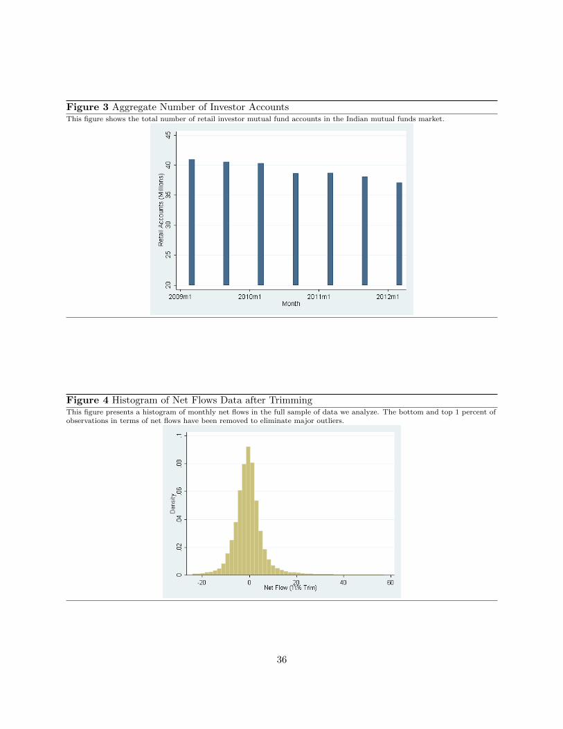
Figure 3 Aggregate Number of Investor AccountsThis figure shows the total number of retail investor mutual fund accounts in the Indian mutual funds market.
Figure 4 Histogram of Net Flows Data after TrimmingThis figure presents a histogram of monthly net flows in the full sample of data we analyze. The bottom and top 1 percent ofobservations in terms of net flows have been removed to eliminate major outliers.
36

Figure 5 Distribution of Fund Observations Across Entry Load LevelsThis figure presents a histogram of monthly fund observations across the levels of entry loads charged in the pre-reformsample (all entry loads were mandated to be equal to zero in the post-reform sample).
Figure 6 Entry Loads on High Vs. Low Fee FundsThis figure shows the average entry loads charged by funds in the high entry load fund group and the low entry load fundgroup. The high entry load group is defined as any fund that charged an entry load of 2.25 percent or higher prior to thereform; the low entry load group is the set of funds that charged entry loads less than 2.25 percent prior to the reform. Thedashed vertical line indicates the date the policy went into force (August 2009). The left panel includes all funds. The rightpanel excludes funds that invested only a small portion of their portfolios in equity.
37

Figure 7 Returns on High Vs. Low Fee FundsThis figure shows the average monthly returns earned in the high and low entry load groups over time. The high entry loadgroup is defined as any fund that charged an entry load of 2.25 percent or higher prior to the reform; the low entry load groupis the set of funds that charged entry loads less than 2.25 percent prior to the reform. The dashed vertical line indicates thedate the policy went into force (August 2009). The left panel includes all funds. The right panel excludes funds that investedonly a small portion of their portfolios in equity.
Figure 8 Assets Under Management in High Vs. Low Fee FundsThis figure presents the logarithm of the assets under management in the high entry load group (solid line) and the low entryload group (dashed line). The high entry load group is defined as any fund that charged an entry load of 2.25 percent orhigher prior to the reform; the low entry load group is the set of funds that charged entry loads less than 2.25 percent prior tothe reform. The dashed vertical line indicates the date the policy went into force (August 2009). The left panel includes allfunds. The right panel excludes funds that invested only a small portion of their portfolios in equity.
38

Figure 9 Average Monthly Net Flows in High Vs. Low Fee FundsThis figure presents the average net flows into funds in the high entry load group (solid line) and the low entry load group(dashed line). The underlying data were trimmed to remove the top and bottom one percent of net-flow observations. Thehigh entry load group is defined as any fund that charged an entry load of 2.25 percent or higher prior to the reform; the lowentry load group is the set of funds that charged entry loads less than 2.25 percent prior to the reform. The dashed verticalline indicates the date the policy went into force (August 2009). The left panel includes all funds, and the right panel excludesincome type funds.
Figure 10 Index Funds: Assets Under Management in High Vs. Low Fee FundsThis figure presents the logarithm of assets under management in the high entry load index fund group (solid line) and thelow entry load index fund group (dashed line). The high entry load group is defined as any fund that charged an entry loadgreater than zero prior to the reform; the low entry load group is the set of funds that charged zero entry loads prior to thereform. The dashed vertical line indicates the date the policy went into force (August 2009).
39

Figure 11 Index Funds: Average Net Flows in High Vs. Low Fee FundsThis figure presents the average net flows in the high entry load index fund group (solid line) and the low entry load indexfund group (dashed line). The high entry load group is defined as any fund that charged an entry load greater than zero priorto the reform; the low entry load group is the set of funds that charged zero entry loads prior to the reform. The dashedvertical line indicates the date the policy went into force (August 2009).
Figure 12 Exit Loads Payable for Exit Within First 30 DaysThis figure presents the average exit load charged by an investor who exited within the first 30 days in funds in the high entryload group (solid line) and the low entry load group (dashed line). The high entry load group is defined as any fund thatcharged an entry load of 2.25 percent or higher prior to the reform; the low entry load group is the set of funds that chargedentry loads less than 2.25 percent prior to the reform. The dashed vertical line indicates the date the policy went into force(August 2009). The left panel includes all funds in the high and low entry load groups. The right panel includes thesub-sample of funds in each group where we were able to obtain exit load data for all the months within a two year window ofthe entry load ban.
40

Figure 13 Exit Loads Payable for Exit Between 31 and 180 DaysThis figure presents the average exit load charged by an investor who exited after 30 days but before 180 days in funds in thehigh entry load group (solid line) and the low entry load group (dashed line). The high entry load group is defined as any fundthat charged an entry load of 2.25 percent or higher; the low entry load group is the set of funds that charged entry loads lessthan 2.25 percent prior to the reform. The dashed vertical line indicates the date the policy went into force (August 2009).The left panel includes all funds in the high and low entry load groups. The right panel includes the sub-sample of funds ineach group where we were able to obtain exit load data for all the months within a two year window of the entry load ban.
Figure 14 Exit Loads Payable for Exit Between 181 and 365 DaysThis figure presents the average exit load charged by an investor who exited after 181 days but before 365 days in funds in thehigh entry load group (solid line) and the low entry load group (dashed line). The high entry load group is defined as anyfund that charged an entry load of 2.25 percent or higher prior to the reform; the low entry load group is the set of funds thatcharged zero entry loads less than 2.25 percent prior to the reform. The dashed vertical line indicates the date the policy wentinto force (August 2009). The left panel includes all funds in the high and low entry load groups. The right panel includes thesub-sample of funds in each group where we were able to obtain exit load data for all the months within a two year window ofthe entry load ban.
41

Figure 15 Exit Loads Collected
This figure presents estimated exit loads based on the aggregate data provided to us by the mutual fund registrar
firm Karvy. The left panel shows exit loads as a percentage of all fees, and the right panel presents the total amount
(in Rs.) of exit loads collected.
Figure 16 Proportion of Households with Outstanding Investments in Major Asset Classes
This figure presents the proportion of households with outstanding investments in various assets in each quarter.
42

Table 1 Summary Statistics: All Funds in the Pre-Reform Period
This table presents summary statistics on low entry load funds, high entry load funds, and all funds. The high entry
load group is defined as any fund that charged an entry load of 2.25 percent or higher prior to the reform; the low
entry load group is the set of funds that charged entry loads less than 2.25 percent prior to the reform. The Total
column includes all funds in the data. Conversions from Indian Rupees to U.S. Dollars are done at 50 rupees per
dollar. Standard deviations of the variable are presented in parentheses below the mean. The significance stars in
the high entry load funds column indicate whether the mean value of the variable is significantly different across the
High and low entry load groups. ***,**,* indicate significance at 1%,5%,10% respectively.
Low Entry Load Fund High Entry Load Fund Total
Entry Load (%) 0.48 2.23*** 1.76(0.68) (0.37) (0.90)
Net Flow (1% Trim) 0.55 0.34 0.39(9.67) (7.69) (8.25)
Assets Under Management (Rupees Millions) 1258.6 2323.2*** 2042.2(5230.1) (4138.5) (4477.3)
Assets Under Management (U.S. Dollars Millions) 25.2 46.5*** 40.8(104.6) (82.8) (89.5)
Log(AUM(t)) 4.71 6.21*** 5.81(2.41) (2.28) (2.41)
Return(t) (%) 0.70 0.80 0.77(5.29) (8.67) (7.92)
Management Expense Ratio 1.10 2.14*** 1.87(0.61) (0.46) (0.68)
Exit Load First 30 Days 0.48 0.69*** 0.64(0.45) (0.53) (0.52)
Exit Load 31 to 180 Days 0.37 0.67*** 0.60(0.44) (0.53) (0.53)
Exit Load 181 to 365 Days 0.33 0.66*** 0.58(0.45) (0.55) (0.54)
Minimum Investment (Rupees) 7854.6 4486.8*** 5358.0(6698.3) (2361.4) (4232.5)
Minimum Investment (U.S. Dollars) 157.1 89.7*** 107.2(134.0) (47.2) (84.6)
# Funds 232 620 852# Fund*Month Observations 5998 16723 22721
43
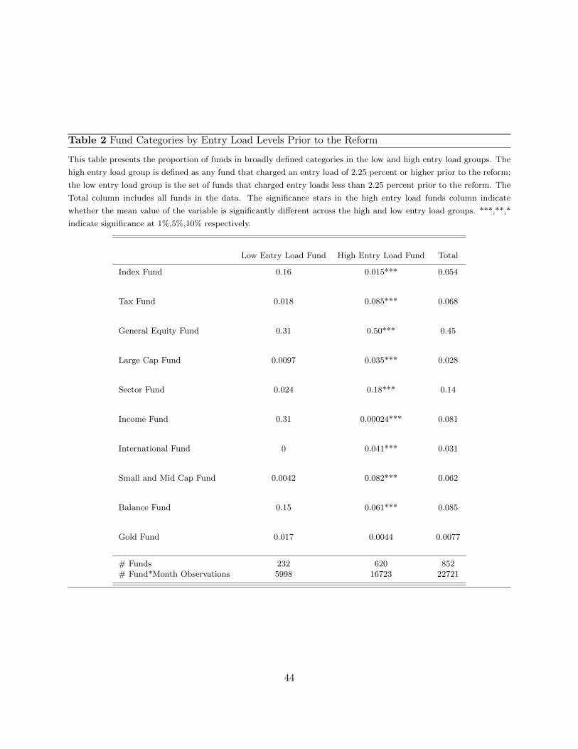
Table 2 Fund Categories by Entry Load Levels Prior to the Reform
This table presents the proportion of funds in broadly defined categories in the low and high entry load groups. The
high entry load group is defined as any fund that charged an entry load of 2.25 percent or higher prior to the reform;
the low entry load group is the set of funds that charged entry loads less than 2.25 percent prior to the reform. The
Total column includes all funds in the data. The significance stars in the high entry load funds column indicate
whether the mean value of the variable is significantly different across the high and low entry load groups. ***,**,*
indicate significance at 1%,5%,10% respectively.
Low Entry Load Fund High Entry Load Fund Total
Index Fund 0.16 0.015*** 0.054
Tax Fund 0.018 0.085*** 0.068
General Equity Fund 0.31 0.50*** 0.45
Large Cap Fund 0.0097 0.035*** 0.028
Sector Fund 0.024 0.18*** 0.14
Income Fund 0.31 0.00024*** 0.081
International Fund 0 0.041*** 0.031
Small and Mid Cap Fund 0.0042 0.082*** 0.062
Balance Fund 0.15 0.061*** 0.085
Gold Fund 0.017 0.0044 0.0077
# Funds 232 620 852# Fund*Month Observations 5998 16723 22721
44

Table 3 All Funds: Comparison of AUM in High vs. Low Entry Load Funds
This table presents regression results on the impact of the entry load ban on assets under management in high
entry load funds versus low entry load funds. The dependent variable is the logarithm of assets under manage-
ment in the fund. The data includes monthly observations over the period April 2006 through June 2012. The
Post Reform dummy variable takes a value of one for the months August, 2009 and afterwards, and zero otherwise.
The High Entry Load Fund variable takes a value of one for funds that charged an entry load of 2.25 percent or
higher in the pre-reform period. Post*High Entry Load Fund is an interaction of the Post Reform variable and the
High Entry Load Fund variable. The variable Lag Ranked Returns Low is defined as min(.5,Rank), where Rank is
defined as the percentile ranking (0 - 100) of the fund’s past six month returns within its category. The variable
Lag Ranked Returns High is defined as Rank−Lag Ranked Returns Low. Family*Post Reform FE are a set of fixed
effects for each fund family separately in the pre-reform period and the post-reform period.
(1) (2) (3) (4) (5)VARIABLES
Post*High Entry Load Fund -0.22* -0.069 -0.074 -0.035 0.040(0.13) (0.088) (0.088) (0.083) (0.083)
Post Reform 0.30** 0.30***(0.12) (0.081)
High Entry Load Fund 1.48***(0.19)
Lag Ranked Returns Low -0.00041(0.00053)
Lag Ranked Returns High -0.0019***(0.00054)
Constant 4.75*** 5.75*** 5.56*** 5.63*** 5.01***(0.16) (0.017) (0.059) (0.052) (0.15)
Observations 47,248 47,248 47,248 47,248 42,074R-squared 0.067 0.929 0.932 0.938 0.946Fund FE NO YES YES YES YESMonth*Year FE NO NO YES YES YESFamily*Post Reform FE NO NO NO YES YESMean Log AUM 5.88 5.88 5.88 5.88 5.95S.D. Log(AUM) 2.40 2.40 2.40 2.40 2.37
45

Table 4 Excluding Income Funds: Comparison of AUM in High vs. Low Entry Load Funds
This table presents regression results on the impact of the entry load ban on assets under management in high
entry load funds versus low entry load funds. The sample excludes income funds that only held a small proportion
of assets in equity. The dependent variable is the logarithm of assets under management in the fund. The data
includes monthly observations over the period April 2006 through June 2012. The Post Reform dummy variable
takes a value of one for the months August, 2009 and afterwards, and zero otherwise. The High Entry Load Fund
variable takes a value of one for funds that charged an entry load of 2.25 percent or higher in the pre-reform period.
Post*High Entry Load Fund is an interaction of the Post Reform variable and the High Entry Load Fund variable.
The variable Lag Ranked Returns Low is defined as min(.5,Rank), where Rank is defined as the percentile ranking (0
- 100) of the fund’s past six month returns within its category. The variable Lag Ranked Returns High is defined as
Rank − Lag Ranked Returns Low. Family*Post Reform FE are a set of fixed effects for each fund family separately
in the pre-reform period and the post-reform period.
(1) (2) (3) (4) (5)VARIABLES
Post*High Entry Load Fund -0.0047 0.13 0.12 0.20** 0.29***(0.15) (0.091) (0.091) (0.096) (0.098)
Post Reform 0.088 0.10(0.13) (0.085)
High Entry Load Fund 1.27***(0.20)
Lag Ranked Returns Low -0.000054(0.00052)
Lag Ranked Returns High -0.0021***(0.00056)
Constant 4.96*** 5.88*** 5.69*** 5.75*** 4.89***(0.18) (0.017) (0.061) (0.053) (0.17)
Observations 43,247 43,247 43,247 43,247 38,886R-squared 0.052 0.931 0.935 0.940 0.948Fund FE NO YES YES YES YESMonth*Year FE NO NO YES YES YESFamily*Post Reform FE NO NO NO YES YESMean Log AUM 5.99 5.99 5.99 5.99 6.04S.D. Log(AUM) 2.35 2.35 2.35 2.35 2.33
46
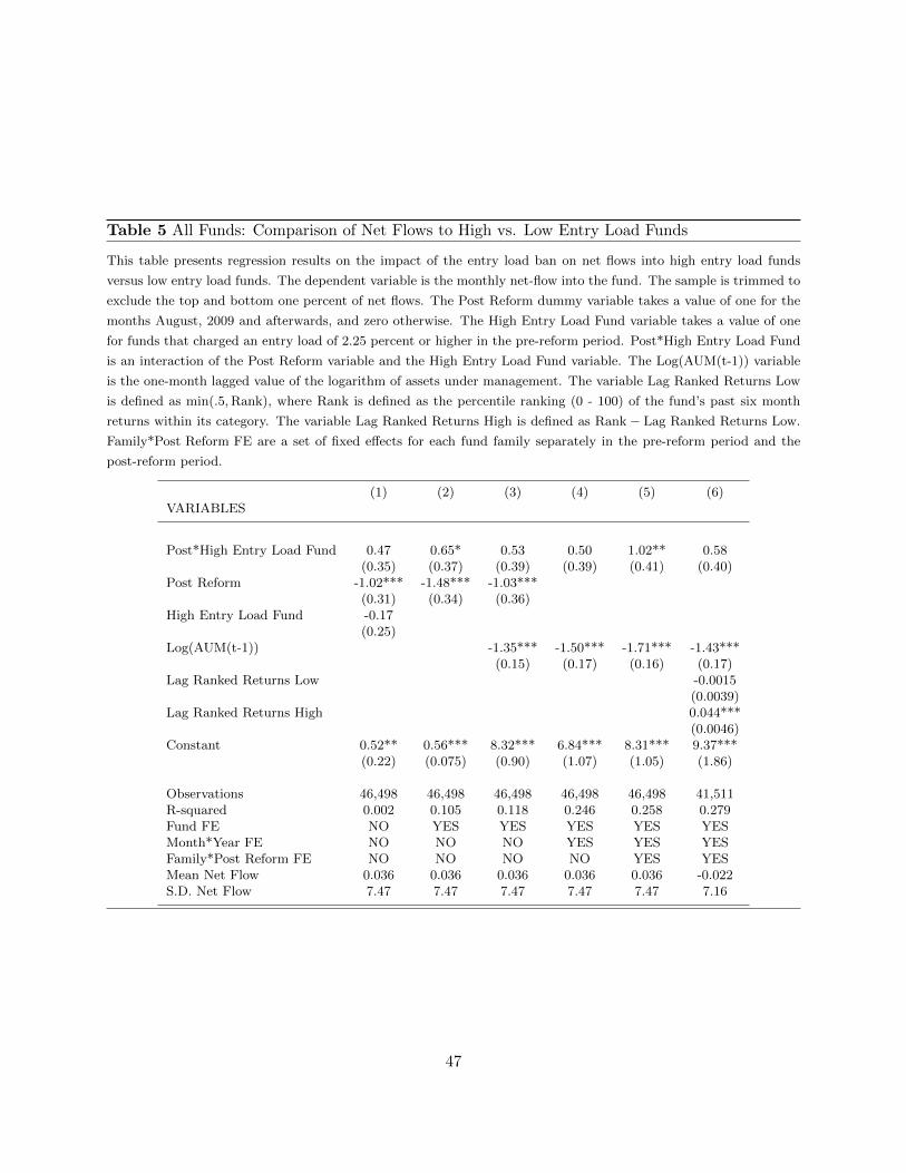
Table 5 All Funds: Comparison of Net Flows to High vs. Low Entry Load Funds
This table presents regression results on the impact of the entry load ban on net flows into high entry load funds
versus low entry load funds. The dependent variable is the monthly net-flow into the fund. The sample is trimmed to
exclude the top and bottom one percent of net flows. The Post Reform dummy variable takes a value of one for the
months August, 2009 and afterwards, and zero otherwise. The High Entry Load Fund variable takes a value of one
for funds that charged an entry load of 2.25 percent or higher in the pre-reform period. Post*High Entry Load Fund
is an interaction of the Post Reform variable and the High Entry Load Fund variable. The Log(AUM(t-1)) variable
is the one-month lagged value of the logarithm of assets under management. The variable Lag Ranked Returns Low
is defined as min(.5,Rank), where Rank is defined as the percentile ranking (0 - 100) of the fund’s past six month
returns within its category. The variable Lag Ranked Returns High is defined as Rank − Lag Ranked Returns Low.
Family*Post Reform FE are a set of fixed effects for each fund family separately in the pre-reform period and the
post-reform period.
(1) (2) (3) (4) (5) (6)VARIABLES
Post*High Entry Load Fund 0.47 0.65* 0.53 0.50 1.02** 0.58(0.35) (0.37) (0.39) (0.39) (0.41) (0.40)
Post Reform -1.02*** -1.48*** -1.03***(0.31) (0.34) (0.36)
High Entry Load Fund -0.17(0.25)
Log(AUM(t-1)) -1.35*** -1.50*** -1.71*** -1.43***(0.15) (0.17) (0.16) (0.17)
Lag Ranked Returns Low -0.0015(0.0039)
Lag Ranked Returns High 0.044***(0.0046)
Constant 0.52** 0.56*** 8.32*** 6.84*** 8.31*** 9.37***(0.22) (0.075) (0.90) (1.07) (1.05) (1.86)
Observations 46,498 46,498 46,498 46,498 46,498 41,511R-squared 0.002 0.105 0.118 0.246 0.258 0.279Fund FE NO YES YES YES YES YESMonth*Year FE NO NO NO YES YES YESFamily*Post Reform FE NO NO NO NO YES YESMean Net Flow 0.036 0.036 0.036 0.036 0.036 -0.022S.D. Net Flow 7.47 7.47 7.47 7.47 7.47 7.16
47

Table 6 Excluding Income Funds: Comparison of Net Flows to High vs. Low Entry Load Funds
This table presents regression results on the impact of the entry load ban on net flows into high entry load funds
versus low entry load funds. The sample excludes income funds that only held a small proportion of assets in
equity. The dependent variable is the monthly net-flow into the fund. The sample is trimmed to exclude the top
and bottom one percent of net flows. The Post Reform dummy variable takes a value of one for the months August,
2009 and afterwards, and zero otherwise. The High Entry Load Fund variable takes a value of one for funds that
charged an entry load greater than or equal to 2.25 percent prior the reform. Post*High Entry Load Fund is an
interaction of the Post Reform variable and the High Entry Load Fund variable. The Log(AUM(t-1)) variable is
the one-month lagged value of the logarithm of assets under management. The variable Lag Ranked Returns Low
is defined as min(.5,Rank), where Rank is defined as the percentile ranking (0 - 100) of the fund’s past six month
returns within its category. The variable Lag Ranked Returns High is defined as Rank − Lag Ranked Returns Low.
Family*Post Reform FE are a set of fixed effects for each fund family separately in the pre-reform period and the
post-reform period.
(1) (2) (3) (4) (5) (6)VARIABLES
Post*High Entry Load Fund 1.10*** 1.50*** 1.62*** 1.59*** 2.41*** 1.87***(0.41) (0.44) (0.44) (0.44) (0.48) (0.47)
Post Reform -1.71*** -2.32*** -2.13***(0.39) (0.41) (0.42)
High Entry Load Fund -0.56*(0.32)
Log(AUM(t-1)) -1.27*** -1.45*** -1.57*** -1.35***(0.15) (0.17) (0.17) (0.18)
Lag Ranked Returns Low -0.0025(0.0037)
Lag Ranked Returns High 0.041***(0.0045)
Constant 0.91*** 0.63*** 8.12*** 6.31*** 7.28*** 7.74***(0.29) (0.078) (0.91) (1.08) (1.09) (1.86)
Observations 42,588 42,588 42,588 42,588 42,588 38,382R-squared 0.004 0.115 0.127 0.273 0.285 0.303Fund FE NO YES YES YES YES YESMonth*Year FE NO NO NO YES YES YESFamily*Post Reform FE NO NO NO NO YES YESMean Net Flow 0.018 0.018 0.018 0.018 0.018 0.0010S.D. Net Flow 7.31 7.31 7.31 7.31 7.31 7.05
48
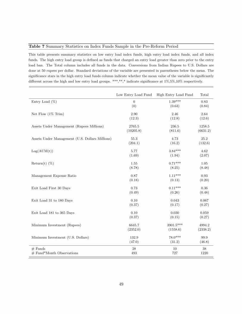
Table 7 Summary Statistics on Index Funds Sample in the Pre-Reform Period
This table presents summary statistics on low entry load index funds, high entry load index funds, and all index
funds. The high entry load group is defined as funds that charged an entry load greater than zero prior to the entry
load ban. The Total column includes all funds in the data. Conversions from Indian Rupees to U.S. Dollars are
done at 50 rupees per dollar. Standard deviations of the variable are presented in parentheses below the mean. The
significance stars in the high entry load funds column indicate whether the mean value of the variable is significantly
different across the high and low entry load groups. ***,**,* indicate significance at 1%,5%,10% respectively.
Low Entry Load Fund High Entry Load Fund Total
Entry Load (%) 0 1.39*** 0.83(0) (0.63) (0.84)
Net Flow (1% Trim) 2.90 2.46 2.64(12.3) (12.8) (12.6)
Assets Under Management (Rupees Millions) 2765.5 236.5 1258.5(10205.8) (811.6) (6631.2)
Assets Under Management (U.S. Dollars Millions) 55.3 4.73 25.2(204.1) (16.2) (132.6)
Log(AUM(t)) 5.77 3.84*** 4.62(1.69) (1.94) (2.07)
Return(t) (%) 1.55 0.71*** 1.05(8.78) (8.25) (8.48)
Management Expense Ratio 0.87 1.11*** 0.93(0.18) (0.13) (0.20)
Exit Load First 30 Days 0.73 0.11*** 0.36(0.49) (0.26) (0.48)
Exit Load 31 to 180 Days 0.10 0.043 0.067(0.37) (0.17) (0.27)
Exit Load 181 to 365 Days 0.10 0.030 0.059(0.37) (0.15) (0.27)
Minimum Investment (Rupees) 6645.7 3901.5*** 4994.2(2352.0) (1558.6) (2338.2)
Minimum Investment (U.S. Dollars) 132.9 78.0*** 99.9(47.0) (31.2) (46.8)
# Funds 28 10 38# Fund*Month Observations 493 727 1220
49

Table 8 Index Funds: Comparison of AUM in High vs. Low Entry Load Funds
This table presents regression results on the impact of the entry load ban on assets under management in high
entry load index funds versus low entry load index funds. The dependent variable is the logarithm of assets under
management in the fund. The data includes monthly observations over the period April 2006 through June 2012.
The Post Reform dummy variable takes a value of one for the months August, 2009 and afterwards, and zero
otherwise. The High Entry Load Fund variable takes a value of one for funds that charged greater than a zero entry
load in the pre-reform period. Post*High Entry Load Fund is an interaction of the Post Reform variable and the
High Entry Load Fund variable. The variable Lag Ranked Returns Low is defined as min(.5,Rank), where Rank is
defined as the percentile ranking (0 - 100) of the fund’s past six month returns within its category. The variable
Lag Ranked Returns High is defined as Rank − Lag Ranked Returns Low.
(1) (2) (3) (4)VARIABLES
Post*High Entry Load Fund 0.65 -0.0088 0.0064 0.053(0.50) (0.47) (0.48) (0.46)
Post Reform -0.27 0.27(0.46) (0.45)
High Entry Load Fund -1.88***(0.42)
Lag Ranked Returns Low -0.0062*(0.0033)
Lag Ranked Returns High -0.0029(0.0030)
Constant 5.75*** 4.65*** 4.15*** 5.18***(0.34) (0.095) (0.29) (0.36)
Observations 2,377 2,377 2,377 2,121R-squared 0.195 0.842 0.852 0.862Fund FE NO YES YES YESMonth*Year FE NO NO YES YESMean Log AUM 4.78 4.78 4.78 4.87S.D. Log(AUM) 1.91 1.91 1.91 1.83
50

Table 9 Index Funds: Comparison of Net Flows in High vs. Low Entry Load Funds
This table presents regression results on the impact of the entry load ban on assets under management in high entry
load index funds versus low entry load index funds. The dependent variable is net flows into the fund. The data
includes monthly observations over the period April 2006 through June 2012. The Post Reform dummy variable
takes a value of one for the months August, 2009 and afterwards, and zero otherwise. The High Entry Load Fund
variable takes a value of one for funds that charged greater than a zero entry load in the pre-reform period.
Post*High Entry Load Fund is an interaction of the Post Reform variable and the High Entry Load Fund vari-
able. The variable Lag Ranked Returns Low is defined as min(.5,Rank), where Rank is defined as the percentile
ranking (0 - 100) of the fund’s past six month returns within its category. The variable Lag Ranked Returns High is
defined as Rank − Lag Ranked Returns Low.
(1) (2) (3) (4)VARIABLES
Post*High Entry Load Fund -0.80 -0.049 -0.26 -1.28(0.92) (1.39) (1.44) (1.32)
Post Reform -2.05** -2.53**(0.81) (1.19)
High Entry Load Fund -0.62(0.95)
Lag Ranked Returns Low 0.050***(0.018)
Lag Ranked Returns High -0.0026(0.031)
Constant 3.01*** 2.67*** -0.42 2.92*(0.81) (0.32) (4.42) (1.55)
Observations 2,240 2,240 2,240 2,016R-squared 0.017 0.085 0.272 0.301Fund FE NO YES YES YESMonth*Year FE NO NO YES YESMean Net Flow 1.37 1.37 1.37 1.35S.D. Net Flow 10.5 10.5 10.5 10.3
51

A Data Appendix
A.1 Terms Used to Identify Funds Dropped from Sample
Any fund with one of the following terms was eliminated from the sample to ensure the sample was
primarily composed of equity funds that retail investors might plausibly invest in:
fixed, institutional, liquid, gilt, treasury, series, income, dividend, fmp, debt, bond,
instn, g-sec, floating, money market, quarterly interval, floater, ultra short term, sun-
daram money fund, rlexible fund, ftp, micf, mgst, mglt, credit opportunities, floating
rate, short term plan, money manager, government securities, deposit fund, cash man-
agement, mmis, savings plus, govt securities, triple ace, short term fund, quarterly
plan, saving advantage, savings advantage, ssif, providend fund, gsf, cash fund, cf-plan,
ust growth, very cautious, sweep, regular savings, medium term plan, long term plan,
monthly interval, half yearly interval, annual interval, hsbc interval, hdfc short term
opportunities, hdfc multiple yield, hdfc high interest, gssif, gfrf, overnight, money plus,
fortis interval, short maturity, insta cash, cash opportunities, life govt, cash manager
52

Table A.1 Summary Statistics: All Funds Excluding Monthly Income Plans in the Pre-ReformPeriod
This table presents summary statistics on low entry load funds, high entry load funds, and all funds. The sample
includes all funds except for monthly income plan type funds. The high entry load group is defined as any fund that
charged an entry load of 2.25 percent or higher prior to the reform; the low entry load group is the set of funds that
charged entry loads less than 2.25 percent prior to the reform. The Total column includes all funds in the data.
Conversions from Indian Rupees to U.S. Dollars are done at 50 rupees per dollar. Standard deviations of the variable
are presented in parentheses below the mean. The significance stars in the high entry load funds column indicate
whether the mean value of the variable is significantly different across the High and low entry load groups. ***,**,*
indicate significance at 1%,5%,10% respectively.
Low Entry Load Fund High Entry Load Fund Total
Entry Load (%) 0.67 2.23*** 1.92(0.72) (0.37) (0.77)
Net Flow (1% Trim) 0.99 0.34** 0.46(10.3) (7.69) (8.27)
Assets Under Management (Rupees Millions) 1597.9 2323.8 2179.1(6165.4) (4138.9) (4623.2)
Assets Under Management (U.S. Dollars Millions) 32.0 46.5 43.6(123.3) (82.8) (92.5)
Log(AUM(t)) 4.93 6.21*** 5.96(2.35) (2.28) (2.35)
Return(t) (%) 0.84 0.80 0.81(6.20) (8.67) (8.24)
Management Expense Ratio 1.01 2.14*** 1.87(0.56) (0.46) (0.68)
Exit Load First 30 Days 0.40 0.69*** 0.64(0.49) (0.53) (0.54)
Exit Load 31 to 180 Days 0.26 0.67*** 0.60(0.45) (0.53) (0.54)
Exit Load 181 to 365 Days 0.23 0.66*** 0.58(0.44) (0.55) (0.55)
Minimum Investment (Rupees) 5510.8 4485.5** 4683.6(4228.4) (2360.1) (2848.3)
Minimum Investment (U.S. Dollars) 110.2 89.7** 93.7(84.6) (47.2) (57.0)
# Funds 166 594 760# Fund*Month Observations 4161 16719 20880
53
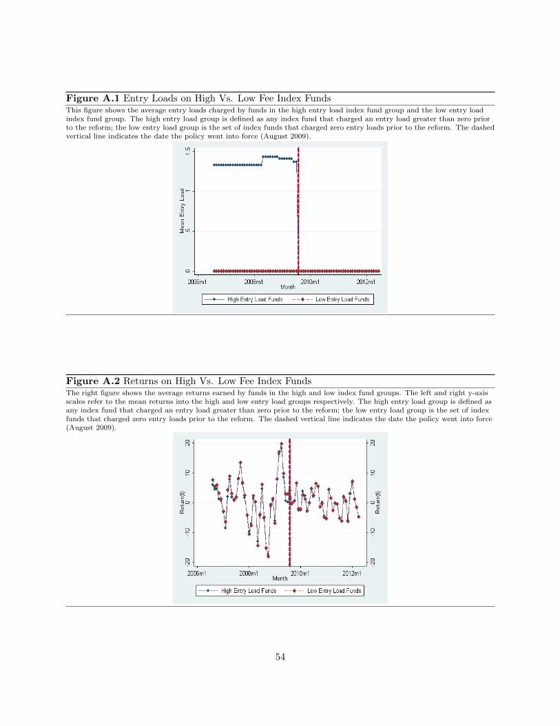
Figure A.1 Entry Loads on High Vs. Low Fee Index FundsThis figure shows the average entry loads charged by funds in the high entry load index fund group and the low entry loadindex fund group. The high entry load group is defined as any index fund that charged an entry load greater than zero priorto the reform; the low entry load group is the set of index funds that charged zero entry loads prior to the reform. The dashedvertical line indicates the date the policy went into force (August 2009).
Figure A.2 Returns on High Vs. Low Fee Index FundsThe right figure shows the average returns earned by funds in the high and low index fund groups. The left and right y-axisscales refer to the mean returns into the high and low entry load groups respectively. The high entry load group is defined asany index fund that charged an entry load greater than zero prior to the reform; the low entry load group is the set of indexfunds that charged zero entry loads prior to the reform. The dashed vertical line indicates the date the policy went into force(August 2009).
54
Top Related