


Languages
Pages
Legal


Disentangling Global Value Chains∗
Alonso de Gortari
First version: August 2016
�is version: September 2018
[latest version]
Abstract
�is paper studies the implications of a key fact: �at many di�erent global value chain (GVC) net-
works aggregate up to the same multi-country input-output data. I argue in favor of networks where
the use of inputs varies depending on the use of output - in contrast to the current literature based on
networks where all output uses the same inputs. I provide evidence for this approach using Mexican
customs data: cars exported to the U.S. use a higher share of imported American inputs than those
exported elsewhere. �is heteroegeneity ma�ers since both quantitative counterfactual estimates and
measures of globalization such as value-added trade vary across GVC networks. I argue that GVCs
are be�er measured when leveraging additional information: incorporating Mexican customs data im-
plies that 30% of U.S. imported Mexican manufactures is U.S. value returning home - higher than the
conventional estimate of 17%.
∗�is paper is based on my 2017 job market paper of the same title and the 2018 paper “Bounding the Gains from Trade”. I am
extremely grateful to my advisors Pol Antras, Elhanan Helpman, and Marc Melitz for their mentorship and guidance through-
out this project, and am also thankful for the comments of numerous participants at seminars and conferences. I gratefully
acknowledge the hospitality of Banco de Mexico, where part of this paper was wri�en. All errors are my own.

1 Introduction
While writing this paper, the North American Free Trade Agreement (NAFTA) was renegotiated for the
�rst time since its inception in 1994, the United Kingdom discussed its potential exit from the European
Customs Union, and the seeds of a possible full-blown trade war between the U.S. and China were sown.
What are the potential costs of these economic shocks? How do they ripple across country borders? Are
the shocks ampli�ed in this age of globalization where over two-thirds of world trade is in intermediate
inputs? Speci�cally, would a 25% tari� on imported Mexican vehicles - as considered by the current U.S.
federal administration - hurt the American worker more or less depending on the share of American value
built into these cars? Further, if Mexican car exports to the U.S. rely heavily on American value-added - as
suggested by anecdotal evidence - why is this so? �roughout the next pages, I will argue that, addressing
these questions requires �rst developing a more accurate, systematic, understanding of the nature of the
global value chains (GVCs, henceforth) underlying world trade than has so far been achieved.
In a nutshell, this paper is about, �rst, showing that the conventional framework used to study GVCs
may be mismeasuring these objects severely. Second, that this mismeasurement ma�ers because it a�ects
the quantitative exercises carried out by both academics and policymakers to study global trade in a world
of highly fragmented production. And, third, that there is a lot of readily available information (data) that
can help improve measurement and thus provide more precise answers to these questions.
�is paper is based upon one central fact: �at any multi-country input-output dataset - the data
typically used to study GVCs - is consistent with many di�erent GVC networks. With this idea in hand,
the paper makes four main contributions - with one section devoted to each. First, I develop a general
theory of GVCs that can be used to compare how di�erent theories of production prescribe the way in
which GVCs should be constructed from input-output data. Second, I show that an in�nite number of
microfounded GVC models can perfectly replicate any given input-output database and that each delivers
di�erent counterfactual predictions to any shock such as a NAFTA trade war. �ird, I show that any given
database is also consistent with a wide range of values for any measure used to study globalization such
as the U.S. content of imported Mexican goods or the U.S.-China value-added trade balance. Fourth, and
�nally, I argue that information beyond that contained in input-output tables, such as transaction-level
customs data, can be used to complement the former and improve the precision of GVC �ow estimates.
I kick o� in section 2 by developing a general theory of GVCs that can accomodate, with further as-
sumptions, how di�erent classes of microfounded models behave in equilibrium and what implications
they have on GVC �ows. For example, the vast majority of trade models with intermediate inputs assume
that technology features roundabout production in which all of a country-industry’s output is produced
using the exact same input mix.1
While speci�c microfoundations di�er substantially, I show that round-
about production models all have the same implications for how GVC �ows are mapped across stages of
production in equilibrium and thus on how GVC �ows should be constructed from input-output data. �is
class of models thus represent one set of assumptions that can be imposed in order to further restrict the
above general theory of GVCs. However, there are many other ways of doing so.
1Roundabout models come in many varieties, some examples include Krugman and Venables (1995), Eaton and Kortum (2002),
Balistreri et al. (2011), di Giovanni and Levchenko (2013), Bems (2014), Caliendo and Parro (2015), Ossa (2015), Allen et al. (2017).
1
I argue in favor of the class of models featuring specialized inputs - models in which goods sold to
di�erent countries or industries are built with di�erent input mixes and value-added shares. While the
class of roundabout models prescribe a single way of constructing a GVC network from any given input-
output database, imposing the specialized inputs assumptions on the general GVC theory has a di�erent
set of implications in that an in�nite number of GVC networks can be constructed from the same data.
More formally, I show that roundabout models prescribe that GVCs should be constructed recursively
using �rst-order Markov chains while specialized inputs models prescribe higher-order Markov chains.
Specialized inputs are consistent with the modern supply chains in which �rms make complex deci-
sions when deciding where to source inputs at each stage of production and where intermediate input
suppliers customize their goods to be compatible with only speci�c downstream uses. For example, the
lithium ba�ery supplier in Apple’s famously long iPod supply chain manufactures it exactly to the size of
the metal frame while the screen supplier ensures that the touch, color, and dimming capabilities are in
line with Apple’s iOS so�ware (Linden et al. 2011). Today, this form of input compatibility is ubiquitous
(Rauch 1999, Nunn 2007, Antras and Staiger 2012, Antras and Chor 2013) and implies that the type of in-
puts used to produce exports, at the country-industry level, should vary depending on use of output since
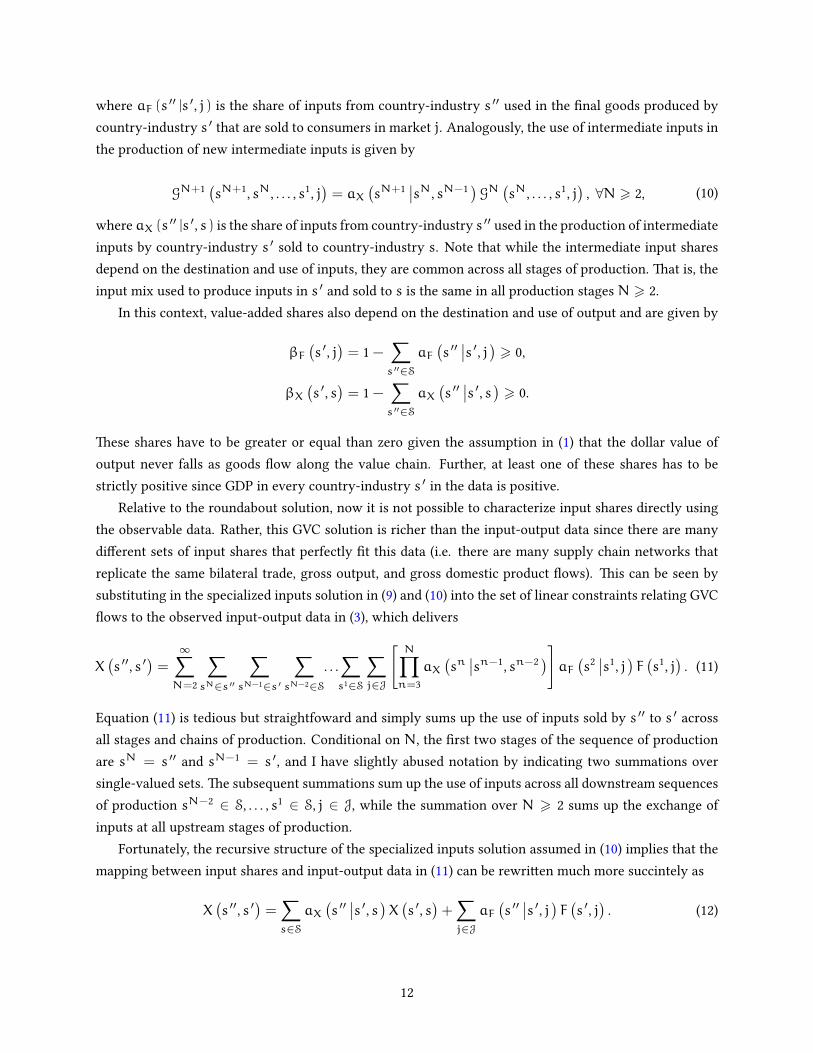
�rms exporting to di�erent countries and industries have di�erent supply chains.2
Indeed, �gure 1 takes
a �rst peek at Mexican customs microdata and shows the distribution of foreign inputs used in Mexico to
produce car exports to the U.S. and Germany. While roundabout models assume that these input mixes
should be exactly the same, in reality the �rms exporting cars from Mexico to the U.S. tend to have supply
chains using U.S. car parts heavily while the �rms exporting to Germany use much fewer U.S. car parts.
Having made the case for specialized inputs, section 3 then shows that quantitative counterfactual
predictions depend crucially on the GVC network. For the sake of clarity, and at the cost of generality,
I illustrate this point with the simplest structural model as given by an extension of a perfect competi-
tion Armington model to specialized inputs - basically, an Armington model where each country-industry
produces a speci�c variety for each market. I show that there is an in�nite ways of parameterizing this
model so that it perfectly replicates any input-output dataset. Moreover, the GVC network ma�ers quan-
titatively since the welfare gains from trade depend on the expenditure share on domestic inputs used for
the production of domestically sold goods. �ese two points imply that mapping the model to di�erent
GVC networks produces di�erent counterfactual estimates following any economic shock - even though
all parameterizations replicate the same input-output data in the benchmark equilibrium. In particular,
this model nests the special case of roundabout production in which the gains from trade are given by the
formula in Arkolakis et al. (2012) and where any counterfactual exercise delivers a single point estimate.3
2Various recent studies suggest that the use of inputs, within country-industries, depend on the downstream use of output.
For example, within-industry exports vary across destinations due to quality (Bastos and Silva 2010), trade regime (Dean et al.
2011), and credit constraints (Manova and Yu 2016). Likewise, the use of imports varies across �rm size (Gopinath and Neiman
2014, Blaum et al. 2017a, 2017b, Antras et al. 2017), multinational activity (Hanson et al. 2005), �rm capital intensity (Scho� 2004),
and the quality of output (Fieler et al. 2017). Further, recent research has made explicit connections between imports and exports
through quality linkages (Bastos et al. 2018), trade participation (Manova and Zhang 2012), and rules-of-origin (Conconi et al.
2018). Finally, production processes vary also in terms of the intensity of labor inputs. Processing trade �rms export lower-cost
labor assembly goods (De La Cruz et al. 2011, Koopman et al. 2012) while �rms exporting to richer countries hire higher-skilled
workers (Brambilla et al. 2012, Brambilla and Porto 2016). �us, value-added shares also di�er depending on the use of output.
3�e Arkolakis et al. (2012) formula does not apply with specialized inputs since the partial elasticity of relative imports from
2

Other13%
CAN3%
DEU4%
JPN
6%
USA
74%
Foreign Inputs inExports to the U.S.
1
Other24%
POL
8% DEU38%
JPN12%
USA18%
Foreign Inputs inExports to Germany
2
Figure 1: Distribution of Foreign Inputs Used In Mexican Final Good Motor Vehicle Exports to
the U.S. and Germany: �e shares are constructed using Mexican customs shipment-level data for
2014; details are discussed in section 2.4.1. In contrast to these charts, the conventional approach
for constructing GVCs assumes common input distributions across destinations.
Further, I show how to use specialized inputs models to construct bounds on any counterfactual esti-
mate - i.e. �nding the upper and lower bounds across all GVC networks that replicate the input-output data
- and show, empirically, that the bounds tend to be quite wide. For example, using the World Input-Output
Database (WIOD), I �nd that a NAFTA trade war where both the U.S. and Mexico increase trade barriers
on each other by 50% delivers a welfare cost to the U.S. between 0.19-0.29% of real income while the cost
form Mexico lies between 3.25-4.66%. In contrast, the special case of roundabout production predicts 0.26%
and 3.68%, respectively. �e goal of this exercise is not to provide highly credible numbers - since the Arm-
ington model is highly simplistic - but rather to illustrate, �rst, the fact that any dataset is consistent with
a range of counterfactual values and, second, that one can construct bounds on them. I conjecture that
future work with richer, more credible, microfoundations will yield similar qualitative implications.4
Analogous to the case of counterfactuals, section 4 shows that measures of globalization - that is,
measures seeking to quantify the current fragmentation of production such as value-added trade (Johnson
and Noguera 2012, Koopman et al. 2014) or average downstreamness (Antras et al. 2012) - also depend
crucially on the GVC network. In particular, in current practice, papers tend to de�ne these measures
directly in terms of input-output analysis (Leontief 1941). In contrast, I de�ne these measures more broadly
using the general theory of GVCs described in section 2 and show that the measures given by input-output
analysis are special cases obtained by further imposing the roundabout assumptions on the general theory.
�is approach is useful because the measures de�ned with input-output analysis are not consistent with
two sources depends on third country trade costs. Hence, the macro-level restriction “the import demand system is CES” fails.
4Examples of richer specialized inputs microfoundations include Yi (2010), Costinot et al. (2012), Antras and Chor (2013),
Fally and Hillberry (2016), Johnson and Moxnes (2016), Antras and de Gortari (2017), and Ober�eld (2018).
3

a world of specialized inputs, but the correct measures can be derived by instead imposing the specialized
inputs assumptions on the general theory. Hence, the general theory provides a common framework for
comparing measures of globalization across di�erent equilibrium theories of production.
I then show how to construct approximate bounds on any measure of globalization and use the WIOD
for 2014 to illustrate that, in practice, value-added trade might be severely mismeasured. For example, a
set of statistics o�en cited during the NAFTA debate were the share of U.S. value-added returning home
through Mexican �nal good imports.5
Higher shares are typically interpreted as proxying a higher cost
of supply chain disruption - i.e. when the U.S. hurts Mexico, this will ripple back and hurt the U.S. more
when it provides more value to these supply chains - and conventional estimates (based on the roundabout
approach) predict that about 17% of the value-added in Mexican manufacturing imports corresponds to U.S.
value returning home. In contrast, I show that the same input-output data is consistent with bounds as
low as 6% and as high as 47%. In other words, in reality Mexican-American supply chains may be much
less or much more integrated depending on how one constructs GVCs. In a second exercise, I focus on the
U.S.-China trade de�cit. As famously shown by Johnson and Noguera (2012), the value-added de�cit based
on the roundabout approach is lower than the gross de�cit since China re-exports a lot of U.S. value-added
back to the U.S. With specialized inputs, however, I �nd that the upper bound is given by a value-added
surplus (i.e. China re-exports a lot more U.S. value-added) but the lower bound is given by a much higher
value-added de�cit (thus, potentially, reversing the key �nding in Johnson and Noguera 2012).
In sum, the key message of sections 2, 3, and 4, is that any given input-output dataset is consistent
with many GVC networks and that the specialized inputs approach together with the bounds approach is
useful for determining the potential mismeasurement that trickles over from the GVC �ows to quantitative
counterfactual estimates and measures of globalization. In other words, since all GVC networks aggregate
up to the same bilateral �ows they all exhaust the information contained in the input-output data. �at is,
there is no further information that can shed light on which speci�c point estimates - be it the roundabout
point estimates, the upper or lower bound, or any point contained therein - are most accurate.
Finally, I devote section 5 to improving measurement, in the sense of obtaining the best informed guess
of the true GVC network underlying input-output data, by incorporating information from other sources.
Speci�cally, I propose an optimization problem that searches over all GVCs consistent with specialized
inputs and a given input-output dataset and chooses the network closest to a set of targets chosen by
the researcher. �is framework is useful when a researcher has information about the underlying GVC
network that is informative but insu�cient for constructing the GVC network directly. For example, in
some countries, there exist datasets including the universe of �rm-to-�rm transactions in which case the
microdata is su�cient for measuring GVC �ows directly.6
More o�en, however, a researcher has some
information such as Mexican customs data that is not su�cient for measuring GVCs directly since it con-
tains no data on domestic transactions. In such a case, the researcher can take a stand on how to use the
Mexican customs data - i.e. her best informed guess about Mexican GVC �ows - by disciplining the targets
5For example, U.S. Secretary of Commerce Wilbur Ross argued in the Washington Post (September 21, 2017) that disrupting
Mexican-American supply chains was not worrisome since Mexican imports contained ‘only’ 16% of U.S. value-added (in 2011).
6In reality, no dataset truly covers the universe of domestic and foreign transactions (in the sense of including data on every
single buyer/seller transaction). However, a Belgian dataset comes quite close; see Tintelnot et al. (2017) and Kikkawa et al. (2017).
4

with this information, and then using the optimization problem to �ll in the missing pieces by ensuring
that the Mexican GVC �ows aggregate up to the input-output data.
I illustrate this approach by using the Mexican customs data to construct the input mix used in each
Mexican manufacturing industry for exports to each destination and industry. In order to use the data, I
take the stand that Mexico only does processing trade - that is, that imported intermediate inputs are used
exclusively for producing exports. While a strong assumption, it is not too far-fetched since processing
trade is widely prevalent in Mexico (De La Cruz et al. 2011). �en, by combining this microdata with the
input-output data or, rather, by disciplining GVC �ows with this informed best guess, I am able to �nd
that the share of U.S. value-added in Mexican manufacturing imports returning home is not 17% as given
by the roundabout model but rather around 30%. Hence, Mexican-American supply chains are much more
integrated than suggested by conventional estimates.
�is measurement framework is quite �exible and can be used to incorporate various forms of infor-
mation into GVC measurement in future work. To begin, my analysis using Mexican customs data does not
incorporate information from other countries but can readily be extended to the la�er case by exploiting
the information in �rm-level datasets across countries. Further, the approach can also incorporate more
abstract forms of information since it only requires that a researcher take a stand on how to use this in-
formation to discipline the optimization targets. For example, rules of origin are widely believed to shape
supply chains in the NAFTA region (Conconi et al. 2018) - and so even if a researcher had no customs-level
data to support this claim, she could obtain a GVC network with highly integrated NAFTA supply chains
by mapping the (abstract) rules-of-origin information into targets of the optimization problem.
From a history of science standpoint, this paper is inspired by Samuelson (1952) which asked how to
measure bilateral trade �ows in the presence of only aggregate export data. �is paper takes the same
idea to the next iteration: How to measure GVC �ows in the presence of only bilateral input-output data?
From a philosophy of science standpoint, this paper is inspired by Popper (1959) and argues for a falsi�able
approach to GVC measurement. �at is, instead of imposing the theoretically-based roundabout approach
outright, I argue in favor of studying GVCs under initially broad sets of plausibly accurate GVCs obtained
through specialized inputs and to then re�ne these estimates as more information becomes available.
2 �e Hunt for GVCs: �e Challenge
�is section provides the GVC framework to be used throughout the rest of the paper to discuss counter-
factuals, measures of globalization such as value-added trade, and measurement in a GVC world. I proceed
in four steps. First, I describe the data contained in a multi-country input-output table. Second, I develop
a general theory that provides notation and a unifying framework for comparing di�erent theories of pro-
duction. I will argue in the rest of the paper that this framework is also useful for deriving explictely the
connection between the literature on structural models and counterfactuals and the literature on measures
of globalization such as value-added trade. �ird, I discuss three speci�c theories of production, two widely
used theories given by a world of ‘only trade in �nal goods’ and a world of roundabout production and a
third more modern theory which I will call specialized inputs, and show how they relate through the use
5
of the general GVC theory. Fourth, and �nally, I argue empirically in favor of the theory of specialized
inputs using Mexican customs shipment-level data and U.S. domestic input-output tables.
2.1 Multi-Country Input-Output Data
Let J denote both the set and number of countries and K the set and number of industries. I de�ne
S = J × K as the set and number of country-industries, with a generic element s ∈ S being a country-
industry denoted as s = {j,k} with j ∈ J and k ∈ K. Multi-country input-output datasets typically contain
data on bilateral intermediate input �ows across two country-industry pairs, with X (s ′, s) the dollar value
of intermediate inputs sold from country-industry s ′ to country-industry s, and �nal good �ows between
a country-industry and consumers, with F (s ′, j) the dollar value of �nal goods sold from country-industry
s ′ to consumers in country j. �ese are the basic building blocks from which all other aggregate moments
are built. For example, gross output of country-industry s ′ equals
GO(s ′)=∑s∈S
X(s ′, s
)+∑j∈J
F(s ′, j)
,
while its gross domestic product equals
GDP(s ′)= GO
(s ′)−∑s∈S
X(s, s ′
).
�ere are currently various sources of multi-country input-output datasets such as those produced by
the World Input-Output Database Project (WIOD), the Global Trade Analysis Project (GTAP), the Institute
for Developing Economies (IDE-JETRO), the Eora Global Supply Chain Database (Eora MRIO), and the
OECD Inter-Country Input-Output Tables (ICIO). Each dataset has its own advantages and limitations and
the analysis in this paper can be readily applied to each. I will focus throughout on the WIOD, which is
the most widely used dataset by the international trade literature, and which is available in its 2016 release
for J = 44 countries, K = 56 industries (17 in manufacturing), and for the years 2000-2014.
2.2 A General GVC�eory
I introduce notation that centers a�ention on GVCs as the central objects of interest instead of parting
directly from a speci�c theory of production. I argue that this general theory can accomodate almost any
speci�c theory of production if one imposes additional assumptions and that this approach is useful since
it provides a unifying framework for comparing the implications of each speci�c theory.
GVC �ows compromise the key building blocks of this theory. Let G (·) denote the dollar value of
production �owing through an initial node across a speci�c ordered set of country-industries all the way
to �nal consumption. To �x ideas, I begin by describing notation assuming a single industry world, that is
S = J. Take three countries j, j ′, j ′′ ∈ J. �en G (j ′, j) denotes the dollar value of �nal consumption goods
that j ′ sells to j while G (j ′′, j ′, j) is the dollar value of intermediate inputs that j ′′ sells to j ′ which j ′ uses
as inputs for goods then sold as �nal consumption to j.
6

More generally, intermediate inputs may be traded at a stage of production that is N ∈ N stages
upstream relative to the production of �nal consumption goods, and I will write a generic truncated GVC
�ow as GN(jN, jN−1
, . . . , j1, j). �e superscript N on GN (·) indicates the dimension of this function, i.e.
N is the number of nodes previous to �nal consumption that are speci�ed. Every node corresponds to a
country with jn ∈ J ∀n and then is only meant to indicate the dimension for which country jn is relevant.
�e �ow GN(jN, jN−1
, . . . , j1, j)
thus indicates the dollar value of inputs from jN sold to jN−1, that jN−1
uses to produce new inputs sold to jN−2, so on and so forth, until the goods arrive at j1 and are put into
�nal goods shipped and sold to consumers in j. Since using apostrophes is cumbersome with large N, in
general I will use the notation G1
(j1, j)
instead of G (j ′, j) and likewise G2
(j2, j1, j
)instead of G (j ′′, j ′, j).
�e extension to a multi-industry world is immediate. Let K be the set of sectors and S = J×K be
the set of country-sectors. GVCs can be de�ned generically as follows.
De�nition 2.1. For any length N ∈ Z+, GN : SN × J → R+
is the function describing truncated GVC
�ows leading to �nal consumption in countries in J through a sequence ofN upstream stages of production
given by an element of SN.
A generic GVC is GN(sN, . . . , s1
, j)
and, as before, I refer to the elements of a country-industry pair as
sn = {jn,kn} with jn ∈ J the country and kn ∈ K the industry of sn ∈ S, where the n is only meant
to indicate the dimension of GN (·) for which sn is relevant. For example: a �ow of length N = 1 could
be G1
(s1
, j)= G1 ({Mexico,cars} , U.S.), the sales of Mexican cars to U.S. consumers, while a �ow of length
N = 2 could be G2
(s2
, s1, j)= G2 ({U.S.,steel} , {Mexico,cars} , U.S.), the sales of U.S. steel in the form of
intermediate inputs that are used exclusively by the Mexican car industry to produce �nal goods sold to
U.S. consumers. Analogously for anyN ∈ Z+and any sequence of production in SN that produces a �nal
good eventually sold to consumers in some country in J.
�e crucial challenge embedded in this theory of GVCs is that the word truncated appears in De�nition
2.1. Speci�cally, GN (·) is a truncated GVC because it only speci�es the �ow throughN stages of production
even though its most upstream stage, sN, also uses inputs and the full chain of production is characterized
by a (potentially) in�nite number of stages of production. �e challenge is thus to develop a theory of
production that links GVC �ows across di�erent stages of production. �at is, take an arbitrary GVC
GN(sN, sN−1
, . . . , s1, j). Since this tells how many inputs are sold from sN to the sequence sN−1 →
· · · → s1 → j then there has to be some relation with the GVC �ow GN−1
(sN−1
, . . . , s1, j)
denoting the
inputs that sN−1itself sells to this sequence of production.
In its most general form, the only restriction I impose is that �ows across di�erent stages of production
must satisfy ∑sN∈S
GN(sN, sN−1
, . . . , s1, j)6 GN−1
(sN−1
, . . . , s1, j)
. (1)
�at is, the right-hand side denotes the value of intermediate inputs sold by sN−1to be used through
the sequence in GN−1
(sN−1
, . . . , s1, j). �e le�-hand side denotes the total value of intermediate inputs,
across all sources sN ∈ S, sold to sN−1and used down this same sequence of production. Imposing equa-
tion (1) thus implies that the total value of inputs purchased by sN−1for a speci�c downstream sequence
of production need be less or equal than the value of the output that sN−1itself produces for that sequence.
7

�is theory is general and can encompass most production processes. It relies only on the key restric-
tion that the dollar value of output not fall as goods �ow down the value chain. Whenever the value of
output increases, which implies that equation (1) holds with strict inequality, I will say that value was
added at theN− 1th stage of production to the inputs purchased from stageN by GN−1
(sN−1
, . . . , s1, j).
For example, this theory assumes that∑s2∈S
G2(s2
, {Mexico,cars} , U.S.
)6 G1 ({Mexico,cars} , U.S.) .
�e right-hand side indicates the dollar value of Mexican cars sold to U.S. consumers and corresponds to
a truncated GVC �ow because the Mexican car industry uses intermediate inputs produced further up-
stream to produce these cars. Meanwhile, G2 ({U.S.,steel} , {Mexico,cars} , U.S.) is the dollar value of U.S.
steel bought as inputs directly in order to produce these exports, so that the summation across all pos-
sible input sources s2 ∈ S yields aggregate input sales to the downstream sequence on the right-hand
side. �e inequality holds strictly if the Mexican car industry adds domestic value-added directly into the
intermediate inputs purchased from the previous stage of production.
I refer to equation (1) as theGVC challengewhich can only be solved by imposing a theory of production
linking GVC �ows across di�erent stages of production. In other words, solving the GVC challenge requires
taking a stand on how GN(sN, sN−1
, . . . , s1, j)
and GN−1
(sN−1
, . . . , s1, j)
relate to each other across all
stages and sequences of production. �roughout the rest of the paper I will restrict a�ention to a static
world in which all goods are produced simultaneously in a single period since this is how input-output data
is typically interpreted in the GVC literature. However, in future work this framework could potentially
incorporate an extension with dynamic production since one can interpret s as a triple of country-industry-
time period in which inputs of past periods �ow down the value chain to be used as inputs in future periods.
2.2.1 Relation to Multi-Country Input-Output Data
Needless to say, GN(sN, . . . , s1
, j)
is not observed directly in input-output tables. If these �ows were ob-
served, then the GVC challenge in equation (1) would be solved trivially since it would rely only on mea-
suring the objects of interest directly. �is does not mean that input-output data is useless, but rather that
it only contains some (non-exhaustive) information about how to solve the GVC challenge in equation (1).
I now show how the GVC �ows relate to this data.
�e �rst thing to note is that input-output data typically provides perfect information about the very
last stage of production, namely that of �nal good production. �is implies that the simplest GVC �ows,
those with N = 1, are observed. Indeed, bilateral �nal good �ows can be de�ned in terms of GVCs as
F(s ′, j)= G1
(s ′, j)
. (2)
�is mapping is the basic building block from which all theories of intermediate input trade will build
upon since this is the only part of the supply chain that is observed directly in input-output data.
Second, bilateral intermediate input �ows are much more complicated since they aggregate the dollar
8

value of inputs traded across two country-industries across all stages of the supply chain. �e relation
between these aggregate �ows and GVC �ows is given by
X(s ′, s
)=
∞∑N=2
∑sN−2∈S
· · ·∑s1∈S
∑j∈J
GN(s ′, s, sN−2
, . . . , s1, j)
. (3)
�e �ow GN(s ′, s, sN−2
, . . . , s1, j)
is the value of inputs from s ′ sold to s at the Nth stage of production
and to be used through a speci�c downstream sequence of production. Summing up across sN−2 ∈ S, …,
s1 ∈ S, j ∈ J thus delivers the aggregate value of inputs from s ′ sold to s at the Nth stage of production
used across all downstream sequences of production. �e �rst summation acrossN > 2 then sums up the
value of inputs traded across all stages of the supply chain. �is aggregate value is thus what is typically
reported in input-output tables.
Speci�c theories of production provide a guide for disentangling GVC �ows across di�erent stages of
production while taking into account the observed input-output data. �at is, since G1 (s ′, j) is observed,
any theory of production needs to take a stand on how to disentangle the GVC �ows GN(sN, . . . , s1
, j)
for
all N > 2 taking into account the restrictions in equation (1) and the fact that a lot of the information is
potentially lost in the aggregation into bilateral intermediate input �ows in equation (3).
2.3 Two Old Solutions, and One New One
I now discuss three possible solutions to the GVC challenge. �e �rst corresponds to a theory in which
only �nal goods are traded, this was the standard GVC theory a few decades ago. �e second corresponds
to the benchmark GVC theory used presently, both in structural models and in terms of literature on
measures of globalization, which incorporates intermediate inputs albeit in a very simpli�ed manner. �e
third corresponds to a new solution which takes seriously the fact that, in reality, supply chain networks
are very complex and that most of this richness is o�en lost through the aggregation into input-output
data. Each subsequent solution is more general and nests the previous one.
Importantly, the theories of production I now discuss require only specifying how the theory behaves in
equilibrium since the input-output data is always interpreted as an equilibrium in the real world. In the rest
of the paper, thinking about counterfactuals will require digging deeper into the speci�c microfoundation
underlying these solutions since one needs to account for how the equilibrium changes a�er a given shock.
In contrast, for the purposes of both studying measures of globalization and improving measurement,
though, specifying how the theory behaves in equilibrium is su�cient.
2.3.1 �e ‘Only Trade in Final Goods’ Solution
�e simplest solution to disentangling GVCs in (1) is to assume that GVC linkages are non-existent. In
other words, parting from the observed GVCs G1
(s1
, j)
assume that the mapping into previous stages of
production at N > 2 is given by
GN(sN, sN−1
, . . . , s1, j)= 0, (4)
9

across any sequence of production. Substituting into the de�nition of intermediate input �ows in equa-
tion (3) implies that for all country-industry pairs s ′ and s
⇒ X(s ′, s
)= 0,
since intermediate inputs are not used at any stage of production. Hence, this system of GVC �ows im-
plies that every dollar of �nal output is made up entirely of domestic value-added created at the most
downstream stage of production
⇒ GO(s ′)= GDP
(s ′)=∑j∈J
G1(s ′, j)=∑j∈J
F(s ′, j)
.
�ese assumptions are extreme and at odds with today’s global economy since over two-thirds of world
trade is in intermediate inputs. Indeed, most datasets report X (s ′, s) > 0 for the majority of country-
industry pairs so that this GVC characterization cannot be squared with current data. However, these
restrictions were still widely imposed even a few decades ago. For example, both the modern version of
the Armington model developed by Anderson (1979) and the classical Ricardian model of Dornbusch et al.
(1977) assume that intermediate inputs play no role so that both models can be characterized, in equilib-
rium, by this GVC representation. While this paradigm is less prevalent today, it is an useful starting point
for showing how to map more complex theories of international trade into the above GVC framework.
2.3.2 �e Roundabout Solution
Disentangling GVCs in the presence of intermediate input trade is much more complex since, in principle,
there are many theories of production that can solve the GVC challenge in equation (1). �is observation
motivates this paper since, so far, the literature has largely focused on a solution in which every single
dollar of output within each country-industry is produced using the exact same input mix. Formally, the
mapping is solved by assuming the existence of a set of technical coe�cients a (s ′ |s) denoting the share of
inputs from s ′ used by s to produce output at any stage of production and for any sequence of production.
Parting from the observed GVCs, G1
(s1
, j), the mapping into previous stages of production at N > 2 is
given by
GN(sN, sN−1
, . . . , s1, j)= a
(sN∣∣sN−1
)GN−1
(sN−1
, . . . , s1, j)
. (5)
Rearranging, any GVC �ow can thus be characterized entirely by �nal good �ows and the technical coef-
�cients as
⇒ GN(sN, sN−1
, . . . , s1, j)=
N∏n=2
a(sn∣∣sn−1
)F(s1
, j)
. (6)
Substituting into the relation between GVC �ows and intermediate input �ows in (3), it is straightfor-
ward to see that the following relation holds
⇒ X(s ′′, s ′
)= a
(s ′′∣∣s ′ )
∑s∈S
X(s ′, s
)+∑j∈J
F(s ′, j) .
10

In other words, since X (s ′, s) and F (s ′, j) are observed in input-output data, this theory of production can
only be squared with the data if the technical coe�cients are given by
⇒ a(s ′ |s
)=X (s ′, s)
GO (s). (7)
�e expenditure by s on inputs from s ′ is simply given by aggregate value of inputs purchased from s ′
relative to gross output. Since gross output is typically larger than aggregate intermediate input purchases,
this implies that every dollar of output of s has a share of domestic value-added given by
⇒ β (s) = 1 −∑s ′∈S
a(s ′ |s
)=GDP (s)
GO (s). (8)
�e roundabout solution has two very useful properties. First, it incorporates intermediate inputs,
whereas the previous ‘only trade in �nal goods’ solution did not. Second, it is so highly tractable that the
measurement problem regarding how to disentangle GVCs is completely eliminated as long as one has
input-output data at hand. Roundabout production implies that any GVC �ow in (6) is characterized by
�nal good �ows and the technical coe�cients, but since the la�er are characterized by input-output data
as well in (7), then any GVC �ow is fully and uniquely characterized by input-output data.
In other words, any microstructure with roundabout production has GVCs that can be characterized,
in equilibrium, by the mapping in (6), and this is equivalent, in terms of measurement, to input-output
analysis. As is well known, the la�er is a measurement framework that leaves no degrees of freedom open
to the researcher since it is fully characterized by input-output data. Importantly, though, while input-
output analysis is o�en de�ned directly as a set of input and value-added shares given by (7) and (8), I
derived these input shares from �rst principles in the sense that I imposed assumptions on the mapping of
GVCs across di�erent stages of the supply chain in (5) and then derived the input shares as an implication.7
�is la�er approach is more useful since it parts from a general theory of GVCs, consistent with many
di�erent theories of production, and in which di�erent measurement frameworks can be contrasted in
terms of the additional assumptions imposed in order to disentangle GVCs from the observable data.
2.3.3 �e Specialized Inputs Solution
�e specialized inputs solution departs from the roundabout solution and assumes that the use of inputs
depends on the destination of output and the use of output, both in terms of whether goods are sold as
�nal goods or intermediate inputs and to which industry they are sold to as inputs in the la�er case. �e
GVC �ow of inputs used directly for the production of �nal goods is thus given by
G2(s2
, s1, j)= aF
(s2
∣∣s1, j)F(s1
, j)
, (9)
7Input-output analysis is typically described using matrix algebra. Imposing the GVC mapping (5) on the de�nition of bilateral
intermediate input �ows in (3) and using matrix algebra implies that
⇒ X = AF+A2F+ · · · = A [I−A]−1
F,
whereGO = [I−A]−1
F is gross ouput and [I−A]−1
is known as the Leontief inverse matrix.
11
where aF (s′′ |s ′, j) is the share of inputs from country-industry s ′′ used in the �nal goods produced by
country-industry s ′ that are sold to consumers in market j. Analogously, the use of intermediate inputs in
the production of new intermediate inputs is given by
GN+1(sN+1
, sN, . . . , s1, j)= aX
(sN+1
∣∣sN, sN−1)GN(sN, . . . , s1
, j)
, ∀N > 2, (10)
where aX (s ′′ |s ′, s) is the share of inputs from country-industry s ′′ used in the production of intermediate
inputs by country-industry s ′ sold to country-industry s. Note that while the intermediate input shares
depend on the destination and use of inputs, they are common across all stages of production. �at is, the
input mix used to produce inputs in s ′ and sold to s is the same in all production stages N > 2.
In this context, value-added shares also depend on the destination and use of output and are given by
βF(s ′, j)= 1 −
∑s ′′∈S
aF(s ′′∣∣s ′, j) > 0,
βX(s ′, s
)= 1 −
∑s ′′∈S
aX(s ′′∣∣s ′, s) > 0.
�ese shares have to be greater or equal than zero given the assumption in (1) that the dollar value of
output never falls as goods �ow along the value chain. Further, at least one of these shares has to be
strictly positive since GDP in every country-industry s ′ in the data is positive.
Relative to the roundabout solution, now it is not possible to characterize input shares directly using
the observable data. Rather, this GVC solution is richer than the input-output data since there are many
di�erent sets of input shares that perfectly �t this data (i.e. there are many supply chain networks that
replicate the same bilateral trade, gross output, and gross domestic product �ows). �is can be seen by
substituting in the specialized inputs solution in (9) and (10) into the set of linear constraints relating GVC
�ows to the observed input-output data in (3), which delivers
X(s ′′, s ′
)=
∞∑N=2
∑sN∈s ′′
∑sN−1∈s ′
∑sN−2∈S
. . .
∑s1∈S
∑j∈J
[N∏n=3
aX(sn∣∣sn−1
, sn−2)]aF(s2
∣∣s1, j)F(s1
, j)
. (11)
Equation (11) is tedious but straightfoward and simply sums up the use of inputs sold by s ′′ to s ′ across
all stages and chains of production. Conditional on N, the �rst two stages of the sequence of production
are sN = s ′′ and sN−1 = s ′, and I have slightly abused notation by indicating two summations over
single-valued sets. �e subsequent summations sum up the use of inputs across all downstream sequences
of production sN−2 ∈ S, . . . , s1 ∈ S, j ∈ J, while the summation over N > 2 sums up the exchange of
inputs at all upstream stages of production.
Fortunately, the recursive structure of the specialized inputs solution assumed in (10) implies that the
mapping between input shares and input-output data in (11) can be rewri�en much more succintely as
X(s ′′, s ′
)=∑s∈S
aX(s ′′∣∣s ′, s)X (s ′, s)+∑
j∈JaF(s ′′∣∣s ′, j) F (s ′, j) . (12)
12

In words, the right-hand side sums up all the intermediate inputs from s ′′ used by s ′ to produce further
downstream inputs sold to all s ∈ S and �nal goods sold to all j ∈ J. Since this is the total value of inputs
sold from s ′′ to s ′ this has to equal the observed �ow X (s ′′, s ′).
All of the information in input-output data is contained in X (s ′, s) and F (s ′, j). �us, any set of input
shares aX (s ′′ |s ′, s) and aF (s′′ |s, j) satisfying (12) for all bilateral pairs characterize a system of GVC
�ows that perfectly �t the observable data. Crucially, ��ing the data requires imposing S× S restrictions
but the specialized inputs GVC network depends on S× S×(S+ J) input shares. �ese degrees of freedom
imply that there are many di�erent GVC networks that replicate the same observable data.
�e roundabout solution is the knife-edge case of specialized inputs in which the input shares for both
�nal and intermediate inputs are assumed to be common and independent of the use or destination of
output. �at is, in this knife-edge case the share of inputs from s ′′ used by s ′ at any stage of production
equals
aX(s ′′∣∣s ′, s) = aF (s ′′ ∣∣s ′, j) = a (s ′′ ∣∣s ′ ) , ∀s ∈ S and ∀j ∈ J.
And the restrictions in (12) imply that the input shares �t the observable data if and only if
a(s ′′∣∣s ′ ) = X (s ′′, s ′)
GO (s ′),
which are exactly the input shares assumed outright in the roundabout solution or input-output analysis.
2.3.4 Taking Stock
I have discussed three solutions showing how theory can be used to disentangle the GVC challenge de-
scribed in (1). Each subsequent theory is more general than the previous one and all three are useful for
understanding the aggregation issues present in input-output data.
First, a few decades ago, bilateral trade data did not distinguish between intermediate input and �nal
good trade and so, in practice, the data was silent regarding whether the ‘only trade in �nal goods’ solution
was potentially accurate or not. Current input-output datasets, however, show that the majority of world
trade is in intermediate inputs and so are now disaggregate enough to be able to reject this GVC theory.
Second, the roundabout solution incorporates intermediate input �ows but assumes that the use of
inputs is common regardless of the destination or use of ouput and across all stages of production. �is
theory is the knife-edge case that �ts the data perfectly and in a unique way. However, it also implicitely
implies assuming that further disaggregating the data would yield no additional insights or information.
�ird, and �nally, the specialized inputs solution can �t the data perfectly in many ways and thus
implicitely assumes that there is important information that is hidden by the aggregation present in input-
output datasets. �e rest of the paper is concerned with using the specialized inputs solution to understand
the implications of such aggregation in currently available input-output datasets.
As a �nal comment, note that there are many other potential ways of disentangling the GVC map-
ping in (1). For example, a richer form of input specialization could be characterized by input shares
aX (s ′′′ |s ′′, s ′, s) where the input mix used in s ′′ for exports to s ′ is tailored according to the further
downstream production stage at s. More formally, this corresponds to building GVCs recursively using
13

third-order Markov chains while the above specialized inputs and roundabout solutions correspond to the
special cases of second-order and �rst-order Markov chains.8
Alternatively, one could assume intermediate
input trade but that GVCs cannot be characterized recursively and are instead �nite with output at some
stage N > 1 consisting entirely of domestic value-added produced at that stage. I focus throughout the
rest of the paper on the specialized inputs solution since it is, in my view, the most natural and tractable
generalization of the roundabout solution. But the reader should keep in mind that the GVC framework
in (1) can be used to study many other solutions in future research.
2.4 Evidence for Specialized Inputs
2.4.1 Evidence from Firm-Level Data
I now use customs shipment-level data to study the presence of specialized inputs in the sales of a given
country-industry to di�erent export markets. Speci�cally, I use the universe of Mexican customs data for
2014 to impute the type of inputs used in exports to di�erent markets. I proceed in three steps. First,
for each �rm I construct its aggregate intermediate input purchases from each country and its aggregate
exports to each country. Second, I assume the roundabout solution at the �rm-level so that all of a �rm’s
exports have the same input mix.9
�is lets me obtain a measure of the dollar value of imports from
each country used in the exports to each country at the �rm-level. �ird, I take all of the �rms within
a manufacturing industry and compute the aggregate value of imports from a given source used in the
exports to a given destination within a manufacturing industry. �is lets me construct the distribution of
foreign inputs used in exports to each destination market - which should be common across markets if the
roundabout solution were accurate at the industry-level.10
Figure 2 con�rms the prevalence of specialized inputs in Mexican manufacturing �nal good exports at
the level of aggregation consistent with typical multi-country datasets.11
Speci�cally, each chart plots the
distribution of foreign inputs from the four main suppliers and a rest of world remainder (rows) used in
the exports to each of the �ve main export destinations (columns) in the top nine Mexican manufacturing
industries. In other words, the cells across a column represent the distribution of foreign inputs in a speci�c
type of exports and add up to 100%. For example, motor vehicles is Mexico’s main export industry and the
corresponding chart shows that the use of inputs in exports to the U.S. and Germany, Mexico’s main North
American and European trade partners, di�er substantially (i.e these are the distributions in �gure 1).
8A previous version of this paper, de Gortari (2017), shows how to disentangle GVCs using Markov chains of any order.
9Most �rms are multi-product �rms and so di�erent inputs are probably used for di�erent exported products within each
�rm. However, the data has no information on what happens within the �rm so this issue cannot be addressed. Having said this,
assuming the roundabout solution at the �rm-level is a much weaker assumption than assuming it at the industry-level.
10Customs data does not contain domestic purchases so value-added shares cannot be measured at the �rm-level and this
analysis also rests on assuming common value-added shares across �rms within an industry. Imposing the roundabout solution
at the industry-level also assumes this and so, in this respect, this analysis is just as far-fetched as the standard approach.
11�e la�er is an important point since one could de�ne manufacturing industries at the �rm-level and then the distribution of
inputs used in exports to di�erent destinations would be common by construction since I have assumed the roundabout solution at
the �rm-level. However, the charts in �gure 2 are presented at the relevant level of aggregation since, for example, manufacturing
�ows in the WIOD are available for only 17 aggregate manufacturing industries. Going forward, while multi-country datasets are
likely to become more disaggregate over time it is unlikely that these datasets become available at a disaggregate enough level to
be consistent with the roundabout solution at the industry-level anytime soon.
14

BRA DEU GBR JPN USA
CHN
DEU
FRA
USA
ROW
Chemicals
5
5
2
2
2
2
1
1
3
3
5
53
35
42
38
16
18
35
44
42
32
22
17
54
21
CAN CHN DEU JPN USA
CHN
JPN
KOR
USA
ROW
Computers, Electronics
5
7
5
6
8
7
12
2
5
9
38
27
23
39
22
28
32
41
31
14
23
30
43
15
28
BRA CAN CHN DEU USA
CHN
JPN
KOR
USA
ROW
Electrical
7 8
11
11
2
10
8
3
1
5
4
14
24
31
24
31
16
34
25
52
33
55
22
49
20
AUS CAN ESP JPN USA
CAN
CHN
IRL
USA
ROW
Food, Tobacco
1
0
11
4
2
1
5
5
0
1
3
0
3
2
7
14
74 58
35
50
40
34
62
64
24
BRA CAN CHN DEU USA
CHN
DEU
KOR
USA
ROW
Machinery
8
6
12
3
5
10
2
3
414
43
29
54
26
14
39
35
24
16
18
19
23
17
57
19
BRA CAN CHN DEU USA
CAN
DEU
JPN
USA
ROW
Motor Vehicles
3
9
12
5
9
6
6
3
2
12
3
4
6
54
22
20
46
20
69
16
38
18
30
74
13
AUS BRA CAN JPN USA
CAN
CHN
FRA
USA
ROW
Other Transport
12
2
0
8
3
0
12
2
1
11
2
0
5
3
3
9
14
72
31
58
22
63
13
74
80
BRA CAN GBR JPN USA
CHN
ITA
TWN
USA
ROW
Textiles
6
2
12
5
2
3
1 3
5
11
2
2
36
37
19
56
25
26
45
25
24
15
53
70
15
CHN DEU FRA JPN USA
CAN
CHN
DEU
USA
ROW
Wood, Paper
0
1
0
12
0
4
4
1
8
1
1
12
1
52
24
23
28
33
27
48
44
55
35
71
15
Figure 2: Foreign Input Shares in Mexican Manufacturing Exports Across Destinations: Each chart
presents the distribution of foreign inputs from the four main input suppliers and a rest of world re-
mainder (rows) used in the exports shipped to the �ve main export destinations (columns) for each
manufacturing industry (i.e. cells across rows within each column sum up to 100%). �ese nine
manufacturing industries account for 95% of Mexico’s �nal good manufacturing exports. Shares
are constructed using Mexican customs shipment-level data assuming that the roundabout solu-
tion holds at the �rm-level. In contrast to these charts, assuming the roundabout solution at the
industry-level implies common input distributions across export destinations.
Overall, �gure 2 shows substantial heterogeneity in input shares in sales to di�erent destinations and
con�rms the fact that NAFTA supply chains are highly integrated. �e U.S. is always one of the �ve main
export markets and always one of the top four input suppliers. Furthermore, the U.S. tends to have an
outsized role as input supplier in the exports that return to its own market - thus con�rming the widely-
available anecdotal evidence that Mexico-U.S. trade is based heavily on goods that cross the border back
and forth. For example, U.S. inputs account for over 70% of foreign inputs in the exports to the U.S. in four
of these nine manufacturing industries and the share is around or above 50% in all but one.
15

2.4.2 Evidence from Disaggregate Domestic Input-Output Tables
I now use domestic input-output tables to study the presence of specialized inputs in the sales of a given
industry to other industries. For example, the computer and electronics industry produces diverse products
such as semiconductors, o�en sold to downstream electronics producers, and navigation instruments, o�en
sold to ship-building companies. However, since computer and electronics is o�en reported as a whole,
GVC estimates based on the roundabout solution assume that the input mix in goods sold to both the
downstream electronics and the ship-building industries is the same. Domestic tables can be used to proxy
the importance of this type of bias since they are o�en available at di�erent levels of disaggregation.
�e U.S. Bureau of Economic Analysis reports domestic input-output tables for the year 2007 at a level
of disaggregation of both 389 and 71 industrial categories (corresponding to the 6- and 3-digit NAICS
classi�cation). I use this data to study the industry aggregation bias through the following thought exper-
iment: I assume the roundabout solution is accurate at the 389 industry-level, so that all output within a
given industry is built with the same input mix regardless of what industry it is sold to, and then compare
these input shares to the ones implied by the more aggregate data with only 71 industrial categories. If
there were no industry aggregation bias, then the input mix used in the production of each of the 6-digit
industries bundled into a single 3-digit industry should be the exactly same and equal to the aggregate
3-digit input mix. If not, then there is an aggregation bias because industries with di�erent input mixes
are being bundled together − thus breaking the assumption that all output within a given industry, at the
3-digit level, is built with the same input mix, even if it is true at the 6-digit level.
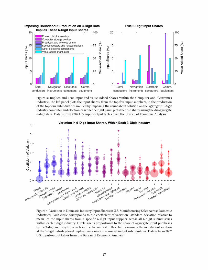
Figure 3 illustrates the industry aggregation bias in the 3-digit computers and electronics industry.
Speci�cally, the la�er is composed of 20 6-digit industries, of which the four largest are semiconductors,
navigation instruments, electronic computers, and communication equipment. Meanwhile, its �ve largest
input suppliers are printed circuit assembly, computer storage devices, broadcast and wireless communi-
cation equipment, semiconductors and related devices, and other electronic components. Figure 3’s le�
panel shows that imposing the roundabout solution on the 3-digit computers and electronics implies that
every product within each 6-digit subindustry is produced with the same input and value-added mix. For
example, computer storage devices accounts for 2.7% of the aggregate output value of the 3-digit comput-
ers and electronics and is thus also the input share used in all 6-digit subindustries. Figure 3’s right panel,
however, uses the more disaggregate 6-digit data to show that input shares vary substantially within each
subindustry. For example, computer storage devices are used intensively as inputs in electronic computers
(15% of output value) but only marginally in the other three plo�ed 6-digit industries.
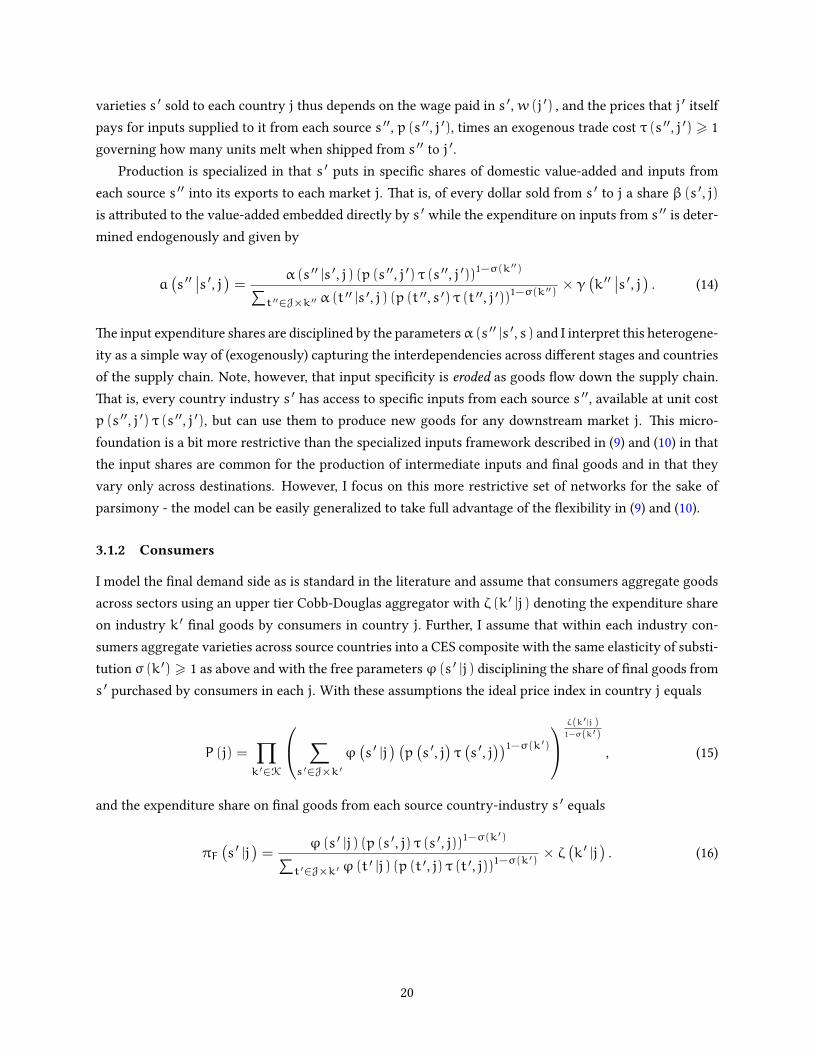
Figure 4 summarizes the industry aggregation bias across all U.S. manufacturing as proxied by the
coe�cient of variation−standard deviation relative to mean−of input shares from each source within each
3-digit code.12
In the absence of aggregation bias, there is no heterogeneity in input shares at the 6-digit
level and the coe�cient of variation is zero. Alternatively, when the aggregation is done across industries
with substantial heterogeneity the coe�cient of variation is large. Each column in �gure 4 corresponds to a
12Speci�cally, for each 3-digit industry k3dig ∈ K3dig
I compute the coe�cient of variation of the input shares a (t |k ) from a
given source t ∈ K6digand across all the 6-digit subindustries k bundled in k3dig
. For example, for the 3-digit industry computers
and electronics, �gure 4 plots one circle for the coe�cient of variation ofa (printed circuit assembly |k ) across all 6-digit subindus-
tries indexed by k, and another circle for a (computer storage devices |k ). Analogously, across all 6-digit suppliers t ∈ K6dig.
16
0
25
50
75
100
Va
lue
-Ad
de
d S
ha
re (
%)
Imposing Roundabout Production on 3-Digit Data
Implies These 6-Digit Input Shares
Semi-
conductors
Navigation
instruments
Electronic
computers
Comm.
equipment
0
5
10
15
20
Inp
ut
Sh
are
s (
%)
Printed circuit assembly
Computer storage devices
Broadcast and wireless comm.
Semiconductors and related devices
Other electronic components
Value-added (right axis)
0
25
50
75
100
Va
lue
-Ad
de
d S
ha
re (
%)
True 6-Digit Input Shares
Semi-
conductors
Navigation
instruments
Electronic
computers
Comm.
equipment
0
5
10
15
20
Inp
ut
Sh
are
s (
%)
Figure 3: Implied and True Input and Value-Added Shares Within the Computer and Electronics
Industry: �e le� panel plots the input shares, from the top �ve input suppliers, in the production
of the top four subindustries implied by imposing the roundabout solution on the aggregate 3-digit
industry computer and electronics while the right panel plots the true shares using the disaggregate
6-digit data. Data is from 2007 U.S. input-output tables from the Bureau of Economic Analysis.
Figure 4: Variation in Domestic Industry Input Shares in U.S. Manufacturing Sales Across Domestic
Industries: Each circle corresponds to the coe�cient of variation−standard deviation relative to
mean−of the input shares from a speci�c 6-digit input supplier across all 6-digit subindustries
within each 3-digit industry. Circle size is proportional to the share of aggregate input purchases
by the 3-digit industry from each source. In contrast to this chart, assuming the roundabout solution
at the 3-digit industry-level implies zero variation across all 6-digit subindustries. Data is from 2007
U.S. input-output tables from the Bureau of Economic Analysis.
17

given 3-digit manufacturing industry, with each circle corresponding to the coe�cient of variation of input
shares from some 6-digit input supplier across the 6-digit subindustries of the 3-digit industry; the size of
each circle is proportional to the importance of each input supplier. Figure 4 reveals one key takeaway:
�ere is substantial variation in input shares within each 3−digit sector. For example, for computers and
electronics the �ve biggest circles are those corresponding to input shares from the sources in �gure 3. �e
largest circle corresponds to other electronic components (the most important supplier) and, as �gure 3
shows, there is relatively li�le variation in input shares so the coe�cient of variation is 0.8. In contrast,
the high variation in computer storage devices visible in �gure 3 yields a coe�cient of variation of 2.7.
Overall, �gure 4 reveals substantial heterogeneity in input shares across sales to di�erent industries
and is informative about specialized inputs in multi-country tables since the la�er are typically available
at an industrial classi�cation level similar to the 3-digit NAICS. Hence, while this exercise cannot be done
with multi-country tables, it is likely that the industry aggregation bias is as prevalent as implied by the
U.S. domestic tables. In particular, since multi-country tables are based on domestic tables, this implies
that assuming common input shares for the U.S. in the la�er leads to distorted supply chain networks.13
3 GVCs and Counterfactuals
A �rst strand of the GVC literature is concerned with understanding the implications of economic shocks,
such as changes in trade barriers, on international trade. In particular, in a seminal contribution, Arkolakis
et al. (2012) (ACR henceforth) argued that, with some assumptions in hand, the welfare gains from trade
can be studied across a variety of di�erent microfoundations with a simple formula depending on the
change in the domestic expenditure share. �ough their benchmark analysis is carried out in a world of
‘only trade in �nal goods’, they show that their results extend to the world of roundabout production.
�is section shows that in richer theories of production, and speci�cally in models with specialized
inputs, the gains from trade vary drastically depending on the GVC network even conditional on a given
input-output dataset. In particular, this section builds on the solutions to the GVC challenge described in
section 2 but goes deeper in that it provides speci�c microfoundations for each theory. �e goal is not to
develop the most general model, but rather to deliver crisp qualitative results and so I focus on the simplest
possible microfoundation. Indeed, I will show how the quantitative implications of any counterfactual
experiment may di�er radically depending on the assumptions made in order to solve the GVC challenge
in (1) and recover the GVC �ows underlying input-output tables. �ough these models are simple, they
provide powerful empirical implications and, while outside the scope of this paper, I conjecture that richer
and, perhaps, more credible microfoundations yield similar qualitative implications.
I proceed in four steps. First, I begin by describing an Armington model with specialized inputs. Sec-
ond, I show that the gains from trade can be represented in terms of a set of domestic expenditure shares
- though, in contrast to ACR, the relevant expenditure shares are the expenditures on domestic inputs
used for the production of domestically-sold goods instead of the aggregate domestic expenditure share.
13�e issue of aggregation in input-output tables motivated an important literature in the 1950’s with several papers developing
conditions under which aggregation is innocuous. �e outlook on whether they might hold in practice was grim, though. In the
words of Hatanaka (1952) and McManus (1956), “�ere is very li�le chance that they will be ful�lled by any model”.
18

Since any input-output dataset is consistent with many networks delivering di�erent domestic expenditure
shares in domestically-sold goods, this implies that any counterfactual exercise may be consistent with a
range of quantitative values. �ird, I show that the reason why the domestic expenditure share is not the
relevant su�cient statistic in a world of specialized inputs is because it does not capture how changes in
trade barriers ripple through supply chain linkages. Fourth, and �nally, I show how to construct bounds
on any counterfactual exercise based on the class of models consistent with the above gains from trade
formulas. I illustrate this empirically with the 2014 WIOD and construct the bounds on the autarky gains
from trade and on the welfare losses across Mexico and the U.S. following a NAFTA trade war.
3.1 Armington Meets Specialized Inputs
I extend the standard Armington model with roundabout production (for example as in Costinot and
Rodrıguez-Clare 2014) to specialized inputs. �ere are J countries and K industries, with each country-
industry s ∈ J×K producing each J di�erentiated varieties − each tailored to a speci�c market. �e
standard roundabout model is the special case in which each country-industry produces the same di�er-
entiated variety for all markets.
�e model is based on �ve main assumptions: (i) both intermediate inputs and �nal goods are produced
with the same technology, (ii) production is specialized in terms of destination country but not destination
industry, (iii) production features constant returns to scale with an upper-tier Cobb-Douglas production
function across labor and intermediate inputs from di�erent sectors and a lower-tier constant elasticity of
substitution (CES) composite of inputs across source countries, (iv) market structure is perfect competition,
(v) the only source of value-added in country j is equipped labor L (j) and commands a wagew (j). While
these restrictions are highly restrictive, the model will prove powerful empirically when going to the data.
3.1.1 Production
Formally, assumptions (iii) and (iv) imply that the model can be described directly in terms of unit prices,
the dual, with the price of a unit of goods from s ′ sold to j given by
p(s ′, j)= w
(j ′)β(s ′,j) ∏
k ′′∈K
∑s ′′∈J×k ′′
α(s ′′∣∣s ′, j) (p (s ′′, j ′) τ (s ′′, j ′))1−σ(k ′′)
γ(k ′′|s ′ ,j )
1−σ(k ′′)
,(13)
where notation is such that country-industry pairs are summarized by s ′′ = {j ′′,k ′′} and s ′ = {j ′,k ′}.
�e upper-tier Cobb-Douglas is characterized by β (s ′, j), the value-added share, and γ (k ′′ |s ′, j), the
expenditure share on sector k ′′ inputs, with β (s ′, s) +∑k ′′∈K γ (k
′′ |s ′, s) = 1. �e lower-tier CES
composite is characterized by two parameters. First, an elasticity σ (k ′′) > 1 governing the degree of
substitutability of the inputs of k ′′ purchased across sources j ′′ ∈ J. �at is, the CES composite of inputs
from an arbitrary sector k ′′ ∈ J is a combination of the inputs from di�erent sources indexed by s ′′ ∈J×k ′′. Second, a set of exogenous input shi�ersα (s ′′ |s ′, j) governing the relative expenditure on industry
k ′′ inputs from each source j ′′ ∈ J, note s ′′ ∈ J× k ′′, satisfying
∑s ′′∈J×k ′′ α (s ′′ |s ′, j) = 1. �e price of
19
varieties s ′ sold to each country j thus depends on the wage paid in s ′,w (j ′) , and the prices that j ′ itself
pays for inputs supplied to it from each source s ′′, p (s ′′, j ′), times an exogenous trade cost τ (s ′′, j ′) > 1
governing how many units melt when shipped from s ′′ to j ′.
Production is specialized in that s ′ puts in speci�c shares of domestic value-added and inputs from
each source s ′′ into its exports to each market j. �at is, of every dollar sold from s ′ to j a share β (s ′, j)
is a�ributed to the value-added embedded directly by s ′ while the expenditure on inputs from s ′′ is deter-
mined endogenously and given by
a(s ′′∣∣s ′, j) = α (s ′′ |s ′, j) (p (s ′′, j ′) τ (s ′′, j ′))1−σ(k ′′)∑
t ′′∈J×k ′′ α (t ′′ |s ′, j) (p (t ′′, s ′) τ (t ′′, j ′))1−σ(k ′′)× γ
(k ′′∣∣s ′, j) . (14)
�e input expenditure shares are disciplined by the parametersα (s ′′ |s ′, s) and I interpret this heterogene-
ity as a simple way of (exogenously) capturing the interdependencies across di�erent stages and countries
of the supply chain. Note, however, that input speci�city is eroded as goods �ow down the supply chain.
�at is, every country industry s ′ has access to speci�c inputs from each source s ′′, available at unit cost
p (s ′′, j ′) τ (s ′′, j ′), but can use them to produce new goods for any downstream market j. �is micro-
foundation is a bit more restrictive than the specialized inputs framework described in (9) and (10) in that
the input shares are common for the production of intermediate inputs and �nal goods and in that they
vary only across destinations. However, I focus on this more restrictive set of networks for the sake of
parsimony - the model can be easily generalized to take full advantage of the �exibility in (9) and (10).
3.1.2 Consumers
I model the �nal demand side as is standard in the literature and assume that consumers aggregate goods
across sectors using an upper tier Cobb-Douglas aggregator with ζ (k ′ |j) denoting the expenditure share
on industry k ′ �nal goods by consumers in country j. Further, I assume that within each industry con-
sumers aggregate varieties across source countries into a CES composite with the same elasticity of substi-
tution σ (k ′) > 1 as above and with the free parametersϕ (s ′ |j) disciplining the share of �nal goods from
s ′ purchased by consumers in each j. With these assumptions the ideal price index in country j equals
P (j) =∏k ′∈K
∑s ′∈J×k ′
ϕ(s ′ |j
) (p(s ′, j)τ(s ′, j))
1−σ(k ′)
ζ(k ′|j )
1−σ(k ′)
, (15)
and the expenditure share on �nal goods from each source country-industry s ′ equals
πF(s ′ |j
)=
ϕ (s ′ |j) (p (s ′, j) τ (s ′, j))1−σ(k ′)∑t ′∈J×k ′ ϕ (t ′ |j) (p (t ′, j) τ (t ′, j))1−σ(k ′)
× ζ(k ′ |j
). (16)
20

3.1.3 Mapping to Input-Output Data
To map the model to the data I build the model’s analogs of the elements of the input-output table. From
the �nal consumption side note that �nal good purchases by consumers in j from source s ′ equals the �nal
good share in (16) times aggregate income
F(s ′, j)= πF
(s ′ |j
)×w (j)L (j) .
�e intermediate input side is constructed by noting that a share of the exports to a given market is at-
tributed to the inputs embedded in them. Aggregate intermediate input exports from s ′′ to s ′ are obtained
by noting that the intermediate input share in (14) delivers the share of inputs from each source in total
exports to each country. �us, aggregate bilateral intermediate input �ows must implicitely satisfy
X(s ′′, s ′
)=∑j∈J
a(s ′′∣∣s ′, j)
∑s∈j×K
X(s ′, s
)+ F
(s ′, j) , (17)
where the right-hand side traces the value of inputs from s ′′ in the exports of both intermediate inputs
and �nal goods from s ′ to j. �e summation then adds up all inputs from s ′′ used by s ′ in exports to all
markets. In practice, input �ows can be computed, conditional on a set of input shares, using this equation
as a �xed point.14
�is model has enough degrees of freedom to �t the data perfectly. Conditional on any vector of
iceberg trade costs τ (s ′, j) > 1 and any elasticity of substitution σ (k) > 1, the parametersϕ (s ′ |j) adjust
to match �nal good �ows, the input mix parameters α (s ′′ |s ′, j) adjust to match intermediate input �ows,
and the Cobb-Douglas and value-added shares β (s ′, j), γ (k ′′ |s ′, j), and ζ (k ′ |j) adjust to match GDP.
More importantly, there are too many degrees of freedom and so there is a continuum of parameterizations
that replicate the same input-output data.
�e roundabout model corresponds to the knife-edge case of no specialization in which exports to
all markets use the same input mix.15
With these restrictions, (17) implies the well-known property of
roundabout models, and of input-output analysis more generally, that input shares are proportional to
bilateral trade shares. �at is if value-added and input expenditure shares do not vary across markets then
there is a single parameterization of the model that �ts the data and delivers the exact same supply chain
14Alternatively, they can be computed directly with linear algebra through X = a [I− a]−1
F. �is approach is reminiscent
of the Leontief inverse matrix but requires a matrix of size S2 × S2instead of size S× S.
15More precisely, I use the term roundabout when referring to production processes in which all output uses the same input
mix and in which the model is implemented literally in that the sectors in the theory are mapped one-to-one to the sectors in
the data (for example Costinot and Rodrıguez-Clare 2014, Caliendo and Parro 2015, and Caliendo et al. 2017). More generally,
the above specialized inputs model can also be interpreted as a more disaggregate multi-industry roundabout model in which
country j has K× J industries in which the goods produced by industry k for country j are only sold to country j. �e mapping
to the data is not one-to-one, however, since the theory has K× J industries per country whereas the data has K. �is paper is
by no means the �rst to take issue with the aggregation in input-output data. Rather, I show how to use the same data in new
ways by constructing bounds that take the (potential) aggregation concerns into account. In the future, the advent of �rm-to-�rm
data will make the cu�ing-edge approaches of Bernard et al. 2018, Lim 2017, and Tintelnot et al. 2017 more widely applicable.
21

network in equilibrium as the one given measured by input-output analysis
if β(s ′, j)= β
(s ′)
, and γ(k ′′∣∣s ′, j) = γ (k ′′ ∣∣s ′ ) , and α
(s ′′∣∣s ′ , j
)= α
(s ′′∣∣s ′ ) ,∀j ∈ J,
⇒ a(s ′′∣∣s ′, j) = a (s ′′ ∣∣s ′ ) = X (s ′′, s ′)∑
t ′′∈S X (t ′′, s ′).
(18)
Hence, while roundabout models may �t the data perfectly, this cannot be interpreted as evidence for the
roundabout approach since many other specialized inputs models also �t it perfectly. Moreover, input-
output data contains no information identifying which networks are most accurate.
3.2 �e Gains from Trade
�is model delivers a su�cient statistics formula that can be used to calculate the change in welfare follow-
ing any change in trade barriers. I derive this formula using the exact hat-algebra approach in four steps.
Speci�cally, let a hat variable denote the ratio of a given variable x across two equilibria, i.e. x = x1/x0, and
let τ (s ′, j) denote the (exogenous) change in trade costs of goods shipped from s ′ to j. As is standard, to
make notation cleaner I assume that domestic trade costs do not change, i.e. τ (s ′, j) = 1 for all s ′ ∈ j×K.
First, I derive the change in expenditure shares. From equation (14), the change in input expenditures
from source s ′′ used by s ′ for goods sold to j as a share of overall expenditure on sector k ′′ inputs equals
a (s ′′ |s ′, j)
γ (k ′′ |s ′, j)=
(p (s ′′, j ′) τ (s ′′, j ′))1−σ(k ′′)∑t ′′∈J×k ′′ a (t
′′ |s ′, j)× (p (t ′′, s ′) τ (t ′′, j ′))1−σ(k ′′). (19)
Analogously, from equation (16), the change in �nal good expenditures consumed from source s ′ by con-
sumers in j relative to overall expenditure on sector k ′ �nal goods equals
πF (s′ |j)
ζ (k ′ |j)=
(p (s ′, j) τ (s ′, j))1−σ(k ′)∑t ′∈J×k ′ πF (t
′ |j) (p (t ′, j) τ (t ′, j))1−σ(k ′). (20)
Both expenditure changes a (s ′′ |s ′, j) and πF (s′ |j) depend on exogenous deep parameters given by the
Cobb-Douglas industry-level expenditure shares and the elasticities of substitutions, the exogenous change
in trade costs, the initial supply chain network as proxied by the original equilibrium’s intermediate input
and �nal good expenditure shares, and the endogenous change in unit prices.
Second, I derive the endogenous change in unit prices in terms of domestic expenditure shares. From
equation (13), the change in unit prices of goods from s ′ sold to j can be wri�en in terms of the change in
input expenditure shares from some source s ′′ using the de�nition in equation (19) as
p(s ′, j)= (w (j))β(s
′,j)∏k ′′∈K
(a(s ′′∣∣s ′, j)− 1
1−σ(k ′′) × p(s ′′, j ′
)τ(s ′′, j ′
))γ(k ′′|s ′,j ), (21)
where each s ′′ may in principle be a source located in any country, that is s ′′ ∈ J× k ′′. As is standard in
the su�cient statistics literature, it proves useful to characterize domestic unit prices in terms of domestic
22

expenditure shares. �at is, take (21) and focus on the domestic industries s ′ ∈ j×K of country j. Domestic
unit prices can be wri�en exclusively in terms of the changes in domestic expenditure shares as follows
p(s ′, j)=∏
s ′′∈j×K
w (j)β(s′′
,j)∏
s ′′′∈j×Ka(s ′′′∣∣s ′′, j)−γ(k ′′′|s ′′ ,j )
1−σ(k ′′′)
δ(k ′′|s ′,j ) (22)
where s ′, s ′′, and s ′′′ all correspond to domestic industries of j. �e change in domestic unit prices thus
depends on the endogenous change in domestic wages and the change in expenditures on domestic in-
termediate inputs used for the production of domestically-sold goods. Further, the change in domestic
prices depends on the change in these expenditures across all stages of the supply chain as captured by the
value-added and Cobb-Douglas expenditure shares and by the auxiliary variable δ (k ′′ |s ′, j) de�ned as
δ(k ′′∣∣s ′, j) = 1[k ′′=k ′] + γ
(k ′′∣∣s ′, j)+ ∑
s ′′′∈j×Kγ(k ′′∣∣s ′′′, j)γ (k ′′′ ∣∣s ′, j)+ . . . .
In other words, δ (k ′′ |s ′, j) is an expenditure share capturing the aggregate (gross) use of inputs from k ′′
used in all upstream stages of production of a purely domestic supply chain for inputs that are eventually
embedded in goods sold by s ′ domestically.16
�ird, I derive the endogenous change in the �nal consumption price index in terms of domestic �nal
good expenditure shares. From equation (15), the change the price index of country j can be wri�en in
terms of the change in �nal good expenditure shares from some source s ′ using the de�nition in equa-
tion (20) as
ˆP (j) =∏k ′∈K
(πF(s ′ |j
)− 1
1−σ(k ′) × p(s ′, j)τ(s ′, j))ζ(k ′|j )
(23)
Fourth, and �nally, substituting the change in unit prices in (22) into the change in the price index in
(23) de�ned in terms of domestic industries s ′ ∈ j × K delivers the following formula for the change in
welfare in terms of the change in domestic expenditure shares
w (j)
ˆP (j)=∏
s ′∈j×K
πF (s ′ |j) 1
1−σ(k ′) ×∏
s ′′∈j×K
∏s ′′′∈j×K
a(s ′′′∣∣s ′′, j)γ(k ′′′|s ′′ ,j )δ(k ′′|s ′ ,j )1−σ(k ′′′)
ζ(k ′|j ) . (24)
�is formula incorporates many of the elements found previously in the literature such as the supply
chain elements from Antras and de Gortari (2017), the domestic expenditure shares from ACR, and the
multi-industry input-output linkages of Caliendo and Parro (2015). Speci�cally, �rst, in a single-industry
world this formula becomes
w (j)
ˆP (j)=
[πF (j |j) a (j |j, j)
1−β(j,j)β(j,j)
] 1
1−σ
, (25)
16Note this expenditure contains value-added counted multiple times. Since the focus is on domestic shares, the Cobb-Douglas
expenditure shares γ (k ′′ |s ′, j ) for country j can be wri�en as a K×K square matrix γwith the corresponding δ (k ′′ |s ′, j ) shares
given by δ = [I− γ]−1
.
23
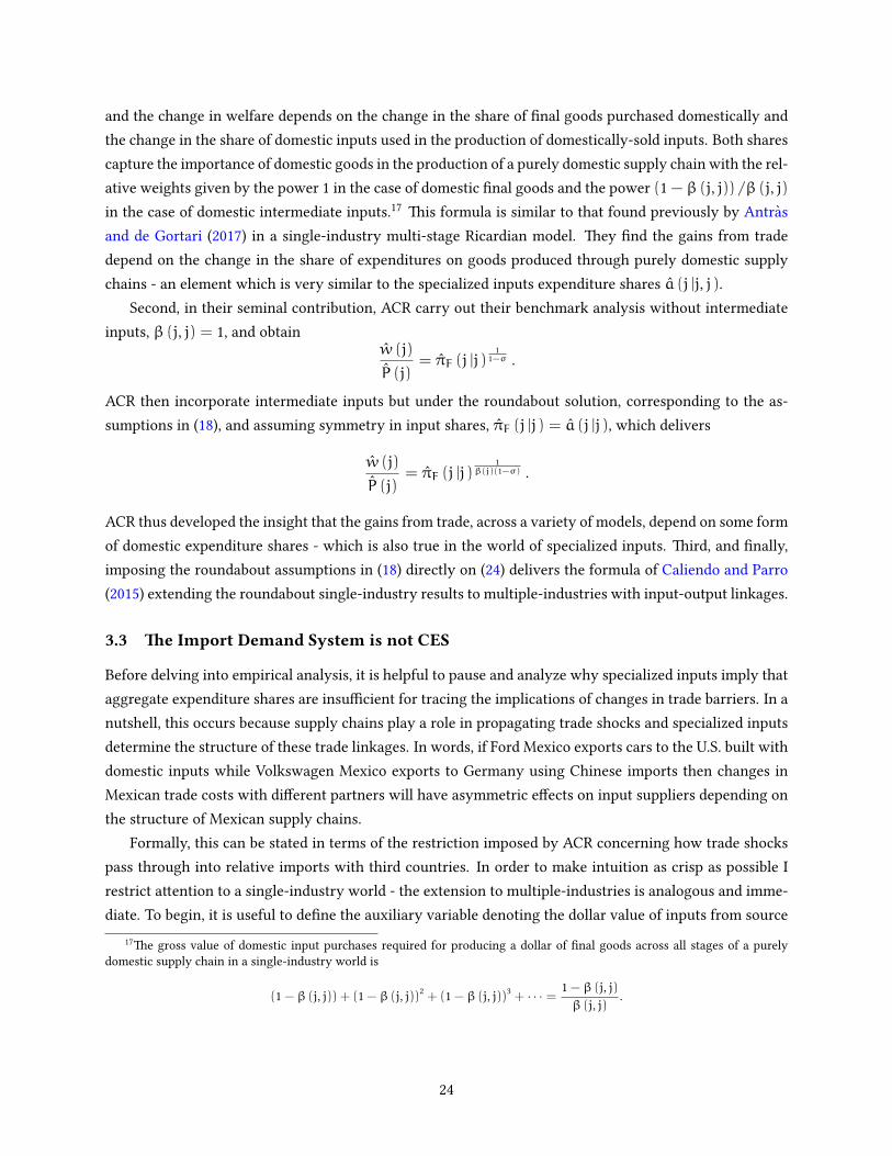
and the change in welfare depends on the change in the share of �nal goods purchased domestically and
the change in the share of domestic inputs used in the production of domestically-sold inputs. Both shares
capture the importance of domestic goods in the production of a purely domestic supply chain with the rel-
ative weights given by the power 1 in the case of domestic �nal goods and the power (1 − β (j, j)) /β (j, j)
in the case of domestic intermediate inputs.17
�is formula is similar to that found previously by Antras
and de Gortari (2017) in a single-industry multi-stage Ricardian model. �ey �nd the gains from trade
depend on the change in the share of expenditures on goods produced through purely domestic supply
chains - an element which is very similar to the specialized inputs expenditure shares a (j |j, j).
Second, in their seminal contribution, ACR carry out their benchmark analysis without intermediate
inputs, β (j, j) = 1, and obtain
w (j)
ˆP (j)= πF (j |j)
1
1−σ .
ACR then incorporate intermediate inputs but under the roundabout solution, corresponding to the as-
sumptions in (18), and assuming symmetry in input shares, πF (j |j) = a (j |j), which delivers
w (j)
ˆP (j)= πF (j |j)
1
β(j)(1−σ).
ACR thus developed the insight that the gains from trade, across a variety of models, depend on some form
of domestic expenditure shares - which is also true in the world of specialized inputs. �ird, and �nally,
imposing the roundabout assumptions in (18) directly on (24) delivers the formula of Caliendo and Parro
(2015) extending the roundabout single-industry results to multiple-industries with input-output linkages.
3.3 �e Import Demand System is not CES
Before delving into empirical analysis, it is helpful to pause and analyze why specialized inputs imply that
aggregate expenditure shares are insu�cient for tracing the implications of changes in trade barriers. In a
nutshell, this occurs because supply chains play a role in propagating trade shocks and specialized inputs
determine the structure of these trade linkages. In words, if Ford Mexico exports cars to the U.S. built with
domestic inputs while Volkswagen Mexico exports to Germany using Chinese imports then changes in
Mexican trade costs with di�erent partners will have asymmetric e�ects on input suppliers depending on
the structure of Mexican supply chains.
Formally, this can be stated in terms of the restriction imposed by ACR concerning how trade shocks
pass through into relative imports with third countries. In order to make intuition as crisp as possible I
restrict a�ention to a single-industry world - the extension to multiple-industries is analogous and imme-
diate. To begin, it is useful to de�ne the auxiliary variable denoting the dollar value of inputs from source
17�e gross value of domestic input purchases required for producing a dollar of �nal goods across all stages of a purely
domestic supply chain in a single-industry world is
(1 − β (j, j)) + (1 − β (j, j))2
+ (1 − β (j, j))3
+ · · · = 1 − β (j, j)
β (j, j).
24

j ′′ that country j ′ uses to produce exports for market j as
X(j ′′∣∣j ′, j) = a (j ′′ ∣∣j ′, j) (X (j ′, j)+ F (j ′, j)) .
From (12), the use of inputs across markets equals aggregate input purchasesX (j ′′, j ′) =∑j∈JX (j ′′ |j ′, j) .
With these variables in hand, the partial elasticity of imports in j ′ from source j ′′ 6= j ′ relative to domestic
input purchases with respect to changes in trade costs with a third country i ′′ 6= j ′ equals
∂ lnX (j ′′, j ′) /X (j ′, j ′)
∂ ln τ (i ′′, j ′)= (1 − σ) 1[j ′′=i ′′] +
∑j∈J
(X (j ′′ |j ′, j)
X (j ′′, j ′)−
X (j ′ |j ′, j)
X (j ′, j ′)
)∂ lnX (j ′ |j ′, j)
∂ ln τ (i ′′, j ′). (26)
�e �rst term captures the direct e�ect on relative imports present when j ′′ = i ′′. In roundabout
models this is the only e�ect. More generally, however, supply chains play a role. �e partial elasticity
∂ lnX (j ′ |j ′, j) /∂ ln τ (i ′′, j ′) captures the change in domestic input purchases due to both a substitution
e�ect capturing a shi� in imports from i ′′ to domestic inputs in exports to j and a supply chain e�ect
derived from the change in downstream production as proxied by the changing level of exports to j. �at
is
∂ lnX (j ′ |j ′, j)
∂ ln τ (i ′′, j ′)= − (1 − σ)a
(i ′′∣∣j ′, j)+ ∂ ln (X (j ′, j) + F (j ′, j))
∂ ln τ (i ′′, j ′).
Further, the term in parenthesis in equation (26) ampli�es/dampens the e�ect on relative imports depend-
ing on the di�erential importance of each export market j for inputs from j ′′ relative to j ′.
In words, if Mexican exports to Germany use mostly Chinese inputs, then a reduction in Mexico-
Germany shipping costs reduces both imports from China and domestic input sales following the substi-
tution towards more German inputs. However, imports from China fall relatively more since exports to
Germany used Chinese inputs intensively. On net, the supply chain e�ect exerts an opposing force and
increases Chinese imports relatively more than domestic sales following the rise in exports to Germany.
Hence, the supply chain e�ect illustrates how changes in trade barriers with third countries a�ect
imports asymmetrically depending on the depth of supply chain integration. In contrast, the roundabout
model is the knife-edge case in which supply chain linkages are symmetric. In other words, when Mexico
uses the exact same input mix to produce all exports this model satis�es what ACR de�ne as the import
demand system being CES in which case the asymmetric e�ect of trade costs on relative imports operating
through supply chain linkages disappears. Formally
�e conditions in (18) ⇒ ∂ lnX (j ′′, j ′) /X (j ′, j ′)
∂ ln τ (i ′′, j ′)= (1 − σ) 1[j ′′=i ′′].
�e empirical evidence on supply chain linkages suggests that specialized inputs play a crucial role in
propagating trade shocks. For example, Barrot and Sauvagnat (2016), Carvalho et al. (2016), and Boehm
et al. (2018) show that supply chain disruptions due to natural disasters are propagated by input speci�city
through trade networks. Increases in suppliers’ marginal costs mostly a�ect tightly-linked �rms, rather
than entire industries symmetrically as in roundabout models.
Finally, note that the gravity equation’s empirical success is not grounds in favor of the roundabout
25

model. I show in appendix section X that gravity regressions fare well across simulations of the special-
ized inputs model even though structural gravity does not hold. While third country trade costs do shi�
bilateral trade �ows, on aggregate the bilateral terms dominate. �e overall e�ect is to a�enuate the trade
elasticity since this model misspeci�cation, i.e. incorrectly assuming structural gravity, is similar to intro-
ducing classical measurement error. �is suggests that gravity-based trade elasticity estimates are biased
downwards when deep supply chain linkages are pervasive.
3.4 Bounding Counterfactuals
3.4.1 Autarky Gains from Trade - Single Industry Bounds
I begin by showcasing the bounds approach to counterfactuals in a highly simplistic se�ing. For now, I
ignore the data’s industrial dimension and assume that there is a single industry per country, i.e. S = J,
and compute the bounds on the gains relative to autarky. In this se�ing, the change in expenditure shares
equal the observed equilibrium’s expenditure shares, i.e. πF (j′ |j ′ ) = πF (j
′ |j ′ ) /1 and a (j ′ |j ′, j ′ ) =
a (j ′ |j ′, j ′ ) / (1 − β (j ′, j ′)) = a (j ′ |j ′, j ′ ) /∑j ′′∈J a (j
′′ |j ′, j ′ ), and since the �nal good shares are ob-
served in the data the only endogenous variables are the input shares a (j ′′ |j ′, j).
�e autarky bounds for country j ′ in any model delivering a welfare formula as in (25) are given by
min/max
∑j ′′∈J a (j
′′ |j ′, j ′ )
1 −∑j ′′∈J a (j
′′ |j ′, j ′ )× ln
a (j ′ |j ′, j ′ )∑j ′′∈J a (j
′′ |j ′, j ′ ),
subject to X(j ′′, j ′
)=∑j∈J
a(j ′′∣∣j ′, j) (X (j ′, j)+ F (j ′, j)) , ∀j ′′ ∈ J,
∑j ′′∈J
a(j ′′∣∣j ′, j) 6 1, ∀j ∈ J,
a(j ′′∣∣j ′, j) > 0, ∀j ′′, j ∈ J.
(27)
�e objective function is a concave transformation of equation (25), while the constraints restrict the search
to expenditure shares that replicate the input-output data. �is optimization problem is relatively easy
to solve since the objective function is well-behaved and the constraints are linear. In the special case
with constant value-added shares, that is β (j ′, j) = β (j ′) for all j ∈ J, this reduces to a simpler linear
programming problem that bounds a (j ′ |j ′, j ′ ) directly.
Crucially, computing bounds requires only zooming in on all possible supply chain networks within
country j ′. �at is, while the world economy depends on J× J× J shares, the optimization solves only for
J× J endogenous variables. �is occurs because this model features li�le specialization in that country
j ′ buys speci�c inputs from j ′′, but can then use them to produce exports to any market. Hence, the
linkages through specialized inputs of country j ′ extend at most from its immediate import suppliers to its
direct export markets. In other words, the observed bilateral trade �ows to and from country j ′ curtail its
specialized network and computing the bounds requires only searching for extremal domestic supply chain
linkages.18
Figure 5 illustrates this in a simple two-country network with constant value-added shares.
18�is breaks down with a higher degree of specialization. For example, suppose that instead a (j ′′′ |j ′′, j ′, j ) disciplines the
26
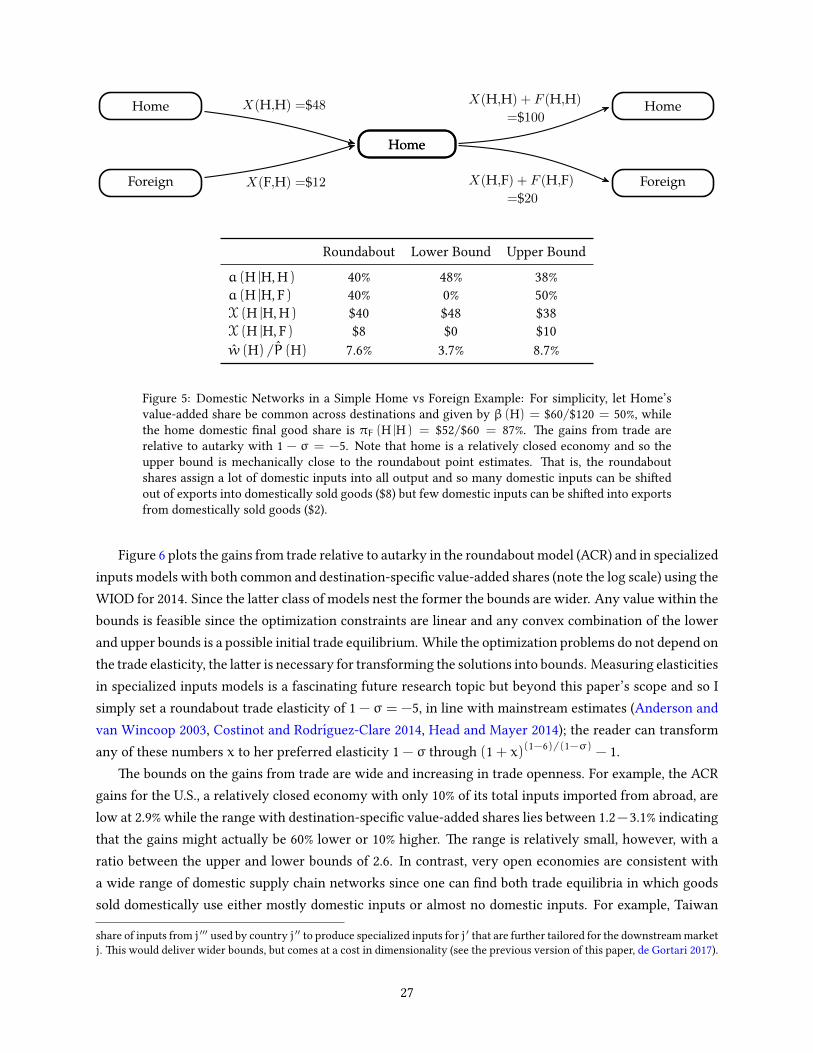
Home
Home Home
Foreign Foreign
Home
X(H,H) =$48
X(F,H) =$12
X(H,H) + F (H,H)
=$100
X(H,F) + F (H,F)
=$20
Roundabout Lower Bound Upper Bound
a (H |H, H) 40% 48% 38%
a (H |H, F) 40% 0% 50%
X (H |H, H) $40 $48 $38
X (H |H, F) $8 $0 $10
w (H) / ˆP (H) 7.6% 3.7% 8.7%
Figure 5: Domestic Networks in a Simple Home vs Foreign Example: For simplicity, let Home’s
value-added share be common across destinations and given by β (H) = $60/$120 = 50%, while
the home domestic �nal good share is πF (H |H ) = $52/$60 = 87%. �e gains from trade are
relative to autarky with 1 − σ = −5. Note that home is a relatively closed economy and so the
upper bound is mechanically close to the roundabout point estimates. �at is, the roundabout
shares assign a lot of domestic inputs into all output and so many domestic inputs can be shi�ed
out of exports into domestically sold goods ($8) but few domestic inputs can be shi�ed into exports
from domestically sold goods ($2).
Figure 6 plots the gains from trade relative to autarky in the roundabout model (ACR) and in specialized
inputs models with both common and destination-speci�c value-added shares (note the log scale) using the
WIOD for 2014. Since the la�er class of models nest the former the bounds are wider. Any value within the
bounds is feasible since the optimization constraints are linear and any convex combination of the lower
and upper bounds is a possible initial trade equilibrium. While the optimization problems do not depend on
the trade elasticity, the la�er is necessary for transforming the solutions into bounds. Measuring elasticities
in specialized inputs models is a fascinating future research topic but beyond this paper’s scope and so I
simply set a roundabout trade elasticity of 1 − σ = −5, in line with mainstream estimates (Anderson and
van Wincoop 2003, Costinot and Rodrıguez-Clare 2014, Head and Mayer 2014); the reader can transform
any of these numbers x to her preferred elasticity 1 − σ through (1 + x)(1−6)/(1−σ) − 1.
�e bounds on the gains from trade are wide and increasing in trade openness. For example, the ACR
gains for the U.S., a relatively closed economy with only 10% of its total inputs imported from abroad, are
low at 2.9% while the range with destination-speci�c value-added shares lies between 1.2−3.1% indicating
that the gains might actually be 60% lower or 10% higher. �e range is relatively small, however, with a
ratio between the upper and lower bounds of 2.6. In contrast, very open economies are consistent with
a wide range of domestic supply chain networks since one can �nd both trade equilibria in which goods
sold domestically use either mostly domestic inputs or almost no domestic inputs. For example, Taiwan
share of inputs from j ′′′ used by country j ′′ to produce specialized inputs for j ′ that are further tailored for the downstream market
j. �is would deliver wider bounds, but comes at a cost in dimensionality (see the previous version of this paper, de Gortari 2017).
27
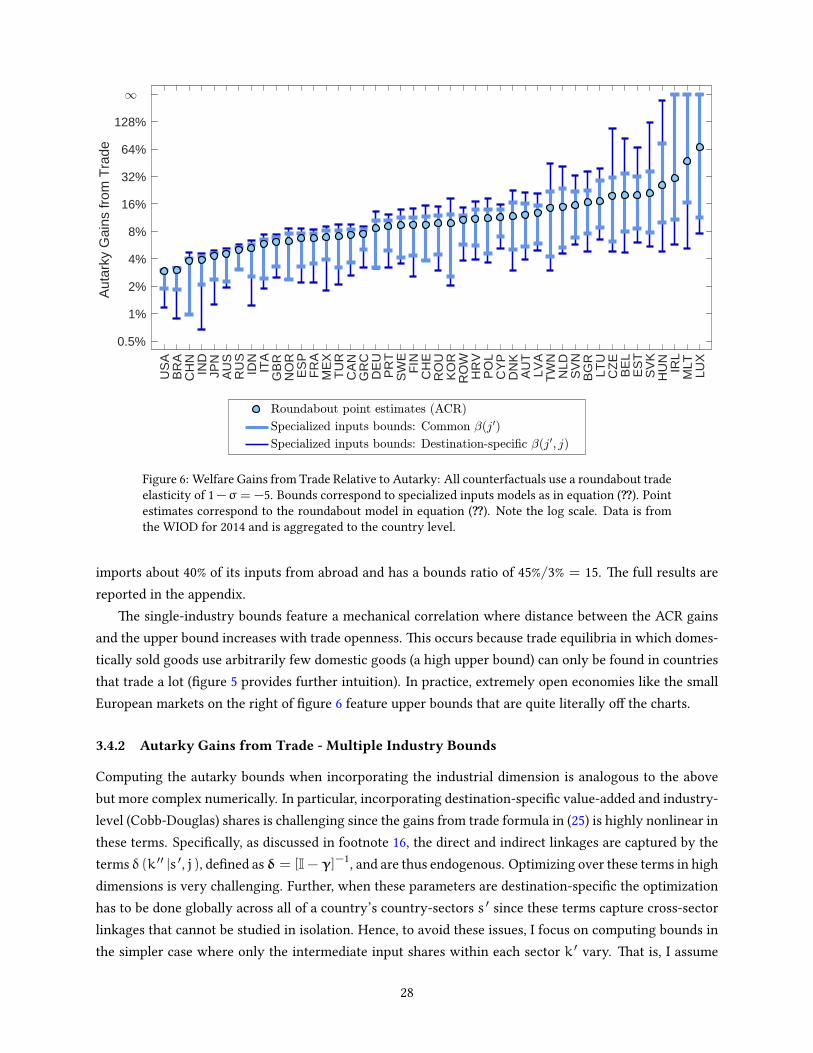
US
AB
RA
CH
NIN
DJP
NA
US
RU
SID
NIT
AG
BR
NO
RE
SP
FR
AM
EX
TU
RC
AN
GR
CD
EU
PR
TS
WE
FIN
CH
ER
OU
KO
RR
OW
HR
VP
OL
CY
PD
NK
AU
TLV
AT
WN
NLD
SV
NB
GR
LTU
CZ
EB
EL
ES
TS
VK
HU
NIR
LM
LTLU
X
0.5%
1%
2%
4%
8%
16%
32%
64%
128%
A
utar
ky G
ains
from
Tra
de
Figure 6: Welfare Gains from Trade Relative to Autarky: All counterfactuals use a roundabout trade
elasticity of 1−σ = −5. Bounds correspond to specialized inputs models as in equation (�). Point
estimates correspond to the roundabout model in equation (�). Note the log scale. Data is from
the WIOD for 2014 and is aggregated to the country level.
imports about 40% of its inputs from abroad and has a bounds ratio of 45%/3% = 15. �e full results are
reported in the appendix.
�e single-industry bounds feature a mechanical correlation where distance between the ACR gains
and the upper bound increases with trade openness. �is occurs because trade equilibria in which domes-
tically sold goods use arbitrarily few domestic goods (a high upper bound) can only be found in countries
that trade a lot (�gure 5 provides further intuition). In practice, extremely open economies like the small
European markets on the right of �gure 6 feature upper bounds that are quite literally o� the charts.
3.4.2 Autarky Gains from Trade - Multiple Industry Bounds
Computing the autarky bounds when incorporating the industrial dimension is analogous to the above
but more complex numerically. In particular, incorporating destination-speci�c value-added and industry-
level (Cobb-Douglas) shares is challenging since the gains from trade formula in (25) is highly nonlinear in
these terms. Speci�cally, as discussed in footnote 16, the direct and indirect linkages are captured by the
terms δ (k ′′ |s ′, j), de�ned as δ = [I− γ]−1
, and are thus endogenous. Optimizing over these terms in high
dimensions is very challenging. Further, when these parameters are destination-speci�c the optimization
has to be done globally across all of a country’s country-sectors s ′ since these terms capture cross-sector
linkages that cannot be studied in isolation. Hence, to avoid these issues, I focus on computing bounds in
the simpler case where only the intermediate input shares within each sector k ′ vary. �at is, I assume
28

that β (s ′, j) = β (s ′) and γ (k ′′ |s ′, j) = γ (k ′′ |s ′ ) are common across all destinations j ∈ J and given
by the data. �e more general framework is le� open for future work.
�e autarky bounds for country j ′ in any multi-industry model delivering a welfare formula as in
equation (24) can be found by solving for the extremal supply chain networks within each pair of sectors
k ′′ and k ′ separately and then incorporating all the solutions into equation (24). Speci�cally, the extremal
domestic shares in country j ′ for the pair of sectors k ′′ and k ′ are found through
min/max a(s ′′∣∣s ′, j ′ ) ,
subject to X(t ′′, s ′
)=∑j∈J
a(t ′′∣∣s ′, j)
∑s∈j×K
X(s ′, s
)+ F
(s ′, j) ,∀t ′′ ∈ J×k ′′,
∑t ′′∈J×k ′′
a(t ′′∣∣s ′, j) = γ (k ′′ ∣∣s ′ ) ,∀j ∈ J,
a(t ′′∣∣s ′, j) > 0,∀t ′′ ∈ J×k ′′, j ∈ J,
(28)
where s ′′ = {j ′,k ′′} and s ′ = {j ′,k ′} are domestic country-industries. Optimization problem (28) is a
linear program with J × J endogenous variables and easy to solve numerically. �e bounds are then
given by solving this problem for the K×K industry pairs and inserting the solutions into the terms
a (s ′′ |s ′, j ′ ) = a (s ′′ |s ′, j ′ ) /γ (k ′′ |s ′ ) and πF (s′ |j ′ ) = πF (s
′ |j ′ ) /ζ (k ′ |j ′ ) in equation (24).
Figure 7 con�rms that the well known fact that multi-industry models deliver larger gains from trade
(Costinot and Rodrıguez-Clare 2014) also holds true for the bounds in the 2014 WIOD. Note, however, that
this does not hold by construction. Rather, the multi-industry bounds are much larger and overlap li�le
with the single-industry bounds because heterogeneity in openness across sectors leads to disproportion-
ate e�ects on the gains from trade. To understand this be�er, imagine a world in which the input-output
data across all industry pairs were identical (in shares) to the aggregate single industry data. Following
Ossa (2015) we know that even in this very special world the gains computed when using the multi-
industry data may be much higher as long as there is heterogeneity in the elasticites of substitution across
industries. However, if there were no heterogeneity then the gains should be the same regardless of the
level of disaggregation. In Figure 7 I have imposed common elasticities across industries and yet the multi-
industry gains are much higher. �is occurs because, in reality, even countries that are relatively closed
on aggregate o�en have some very open industries consistent with many supply chain networks.
Hence, in a world of specialized inputs heterogeneity in openness across industries implies that the
gains from trade may di�er widely depending on the supply chain network even if trade elasticities are
common across industries. In future work, mixing both approaches and incorporating heterogeneity in
elasticites measured in the context of specialized inputs may produce even wider bounds.
3.4.3 Arbitrary Changes in Trade Costs
Ultimately, perhaps the most relevant empirical exercise is computing bounds on counterfactuals based on
real world and policy-motivated events. Relative to the autarky case, however, computing bounds follow-
ing arbitrary changes to trade barriers is much more complex. While describing how to do it theoretically
29

US
A
BR
A
CH
N
IND
JPN
AU
S
RU
S
IDN
ITA
GB
R
NO
R
ES
P
FR
A
ME
X
TU
R
CA
N
GR
C
DE
U
SW
E
FIN
CH
E
KO
R
RO
W
PO
L
DN
K
AU
T
TW
N
NLD
BE
L
IRL
0.5%
1%
2%
4%
8%
16%
32%
64%
128%
A
utar
ky G
ains
from
Tra
de
Figure 7: Welfare Gains from Trade Relative to Autarky, Multiple Sectors: All counterfactuals use
common roundabout trade elasticities 1 − σ (k) = −5 in all sectors. Point estimates correspond to
the roundabout model as in eq X and eq X. Bounds correspond to multi-sector specialized inputs
models as in equation (24). Note the log scale. Data is from the WIOD for 2014 and is aggregated
the J = 30 largest economies and K = 25 sectors per country (see appendix).
is straightforward, in practice it may be hard to solve numerically with current computing power. Fortu-
nately, though, computing approximate bounds is feasible and are informative about the true bounds.
I relegate the formal description of this optimization problem to Appendix Section X and begin by
discussing here the main numerical challenges. First, the counterfactual gains in general depend on the
full supply chain network whereas in the autarky experiments the gains depend only on the domestic
supply chain network. Hence, while the multi-industry autarky bounds relied on solving K×K separate
linear optimization problems of size J× J each, computing bounds for an arbitrary shock to trade barriers
requires solving a single global optimization problem with J×K×J×K×J endogenous variables. Second,
and relatedly, this implies that the objective function is given by the full formula in equation (24) which
is nonlinear. �ird, the constraints are highly nonlinear since they include �xed points for the changes in
unit prices and wages. �ese three points imply the increase in dimensionality makes this problem hard
to solve numerically unless the data is aggregated to few countries and industries.
All is not lost though since, �rst, computing general counterfactuals for a given supply chain network
is straightforward and, second, the specialized inputs framework described above provides a simple way
of constructing supply chain networks conditional on a given input-output dataset. In the special case
of the specialized inputs Armington microfoundation, we need only �nd a set of input shares that satisfy
equation (17) for all pairs of country-sectors. Further, since these constraints are linear then if two supply
30

Figure 8: Approximate Bounds of a NAFTA Trade War: �e le� panel plots the U.S. and Mexico
welfare loss following a 50% increase in trade barriers for goods shipped from Mexico to the U.S
across 10,000 supply chain networks that replicate the WIOD in 2014. Each circle is a supply chain
network constructed as a random linear combination, within each country-sector, of the supply
chain networks corresponding to the autarky specialized inputs lower bound, the roundabout so-
lution, and the autarky specialized inputs upper bound underlying Figure 7. �e right panel plots
the welfare losses when Mexico retaliates and trade barriers also increase by 50% for goods shipped
from the U.S. to Mexico. Note the true bounds on these counterfactuals are wider than these sets.
chain networks replicate a given input-output dataset then any linear combination of these two supply
chain networks will also do so.
Figure 8 looks at the e�ects of a NAFTA trade war between Mexico and the U.S. across the set of supply
chain networks that can be constructed as linear combinations of the supply chain networks underlying
the autarky lower bounds, the roundabout solution, and the autarky upper bounds in �gure 7. Specif-
ically, the le� panel of �gure 8 �rst takes each of these three benchmark networks, then computes the
observed equilibrium (which replicates the 2014 WIOD), and then recomputes the equilibrium following a
50% increase in the trade barriers Mexico faces when exporting goods to the U.S. �en, I take 10,000 linear
combinations of these supply chain networks and redo this exercise while plo�ing each simulation as a
dot; the color of each dot proxies how close it is to the three benchmark networks. �e right panel does
the same exercise except that it assumes that Mexico retaliates and trade barriers for goods shipped from
the U.S. to Mexico also increase by 50%.
�e sets depicted in �gure 8 are narrower than the true bounds, by de�nition, but show that one can
easily �nd sizable deviations to the predictions of a roundabout model.19
In this particular example, the
19�e curious reader may wonder why the points in these sets are not convex combinations of the three benchmark networks.
�ere are two reasons. First, the linear combinations are within industry pairs so, for example, there are some supply chain
31
roundabout model tends to underpredict the costs of NAFTA trade war for Mexico and overpredict for
the U.S. relative to the overall set. Of course, this may not be true in reality since the true supply chain
network corresponds to only one point which may be anywhere in the set and have li�le to do with the
average network. Further, even if we made the heroic assumption that this model represents the true data
generating process in reality, I cannot say whether the true supply chain network is contained within the
depicted sets since these only correspond to approximate bounds and the true bounds may be much wider.
As a word of caution, the magnitudes from this exercise are not to be taken at face value. �e above
model is very stylized and does not incorporate elements such as tari� income, �xed costs of production,
nor monopoly power. Rather, the goal is, �rst, to illustrate in the simplest possible way how quantitative re-
sults may di�er drastically depending on how researchers interpret input-output datasets. �ough outside
the scope of this paper, I conjecture that more complex and richer microfoundations deliver qualitatively
similar results. Second, the goal is to motivate the need for further measurement so that input-output
datasets can be interpreted accurately. By doing this, structural models can then be disciplined by supply
chain networks that are informed by data, and are thus hopefully as close as possible to the true underlying
networks, instead of relying on the theoretically-built roundabout networks.
4 GVCs and Measures of Globalization
A second strand of the GVC literature is concerned with measuring the extent of fragmentation of pro-
duction across borders and stages of the supply chain. �is literature has developed various measures to
be�er capture this fragmentation than those based on traditional statistics such as gross trade �ows. �e
most popular of thses statistics are those based on value-added trade (Hummels et al. 2001, Johnson and
Noguera 2012, Koopman et al. 2014) which aim to capture where value is created rather than where value
is shipped from. A second set of popular statistics are those based on average upstreamness (Fally 2012,
Antras et al. 2012, Antras and Chor 2013) which aim to measure a country’s average position along the
value chain. �ere are many others such as measures of the factor content of trade (Tre�er and Zhu 2010),
value-added exchange rates (Bems and Johnson 2017), international in�ation spillovers (Auer et al. 2017),
and business cycle synchronization (di Giovanni and Levchenko 2010, Johnson 2014b, Duval et al. 2016,
di Giovanni et al. 2017). I will refer to all of these measures generically as measures of globalization.
�is section shows how measures of globalization vary drastically depending on the supply chain net-
work even within a given input-output dataset. In order to sharpen the analysis, I focus throughout on
decompositions of value-added trade but the same ideas hold generally for any of the measures of global-
ization listed above. I proceed in three steps. First, I show that any measure of globalization can be de�ned
using the general theory of GVCs from section 2. �is contrasts with the standard approach in which these
measures are de�ned with a speci�c equilibrium theory of production, mainly the roundabout solution, in
mind. De�ning these more generally proves useful since this permits the comparison of di�erent theories
networks in which the U.S. is close too the lower bound input shares in some industries but close to the upper bound in other
industries. Second, in the autarky case the gains from trade are monotonic in the domestic input shares and so there is a one-
on-one relation between linear combinations (at the country level) and the gains from trade. More generally, this is not the case
since the counterfactual equilibrium depends nonlinearly (and possibly non-monotonically) on the observed equilibrium through
the �xed point in unit prices and wages.
32

of production in terms of their implications on measures of globalization. Second, I show how to compute
bounds on these measures when imposing the specialized inputs solution and compare them to the con-
ventional measures given by the roundabout solution. �ird, and �nally, I illustrate the la�er empirically
with the WIOD and showing how the bounds on the share of U.S. value-added in imported Mexican �nal
goods and the U.S.-China value-added de�cit, two widely studied measures in the GVC literature, are very
wide and thus imply that the conventional roundabout estimates may be highly mismeasured.
A key di�erence between this section on measures of globalization and the previous section on coun-
terfactuals is that here we still need to take a stand on a theory of production in order to do empirical
analysis but we do not need to take a stand on a speci�c microfoundation. �at is, here we still need
to assume that the theory of production is given by either the roundabout or specialized inputs solution.
However, we need only assume that the theory of production delivers a certain type of supply chain net-
work in equilibrium but can disregard the speci�c microfoundation that delivers such equilibrium. In this
sense, this section is much more �exible than the previous one in that it requires much fewer assumptions.
4.1 Decomposing Value-Added Trade
Decomposing �nal good consumption into where each dollar of value-added was produced is useful in
order to understand how �nal consumption in some country, say the U.S., is linked to the production
capacity of another, say China, through �nal good exports of a third country, say Mexico. Further, this
decomposition can be used to construct value-added trade imbalances by taking the di�erence between
the aggregate value of, say, Chinese value-added consumed in the U.S. arriving through �nal good exports
of any country and the aggregate value of U.S. value-added that is eventually consumed in China. More
speci�cally, in the most general form, the dollar value of value-added from s ′′ that arrives through �nal
good exports of s ′ and is consumed in country j is de�ned as
VA(s ′′∣∣s ′, j) = 1[s ′′=s ′]
G1(s ′, j)−∑s2∈S
G2(s2
, s ′, j)
+
∞∑N=3
∑sN−2∈S
· · ·∑s2∈S
GN−1(s ′′, sN−2
, . . . , s2, s ′, j
)−∑sN∈S
GN(sN, s ′, sN−2
, . . . , s2, s ′, j
) .
(29)
�e �rst term imputes value-added created directly at the assembly stage, appearing only if s ′′ = s ′, while
the remaining terms impute value-added created by s ′′ at all further upstream stages of production and
which eventually arrives, through any possible sequence, to s ′ to be shipped to consumers in j.
Value-added trade can be rewri�en in terms of a model’s equilibrium supply chain network once one
takes a stand on the theory of production solving the GVC challenge in (1). To exemplify this, I begin
by showing how this decomposition simpli�es once one assumes the specialized input solution in (9) and
(10), and then show how it relates to the other solutions. To make the exposition clearer, I derive the
decomposition separately for the value-added created at each stage N. First, the value-added by s ′′ at the
33

most downstream stage, N = 1, into �nal good sales of s ′ to j equals
VA1(s ′′∣∣s ′, j) = 1[s ′′=s ′]βF
(s ′, j)F(s ′, j)
, (30)
where the super-index on VA is meant to index the stage at which this value-added is produced. Clearly,
since the most downstream stage is that of �nal production, s ′′ adds value-added to �nal good sales of s ′
if and only if s ′′ = s ′, and the decomposition is given by the share of value-added βF (s′, j) in each dollar
of output times the sales of �nal goods. Second, the value-added generated at the N = 2 upstream stage
is given by
VA2(s ′′∣∣s ′, j) = βX (s ′′, s ′)aF (s ′′ ∣∣s ′, j) F (s ′, j) , (31)
and the decomposition is now given by the value-added share in intermediate inputs βX (s ′′, s ′) times the
level of inputs from s ′′ used in the �nal good sales from s ′ to j. �ird, and �nally, the decomposition of
value-added for any further upstream stage N > 3 is given by
VAN(s ′′∣∣s ′, j) = ∑
sN−1∈S
. . .
∑s2∈S
βX(s ′′, sN−1
) [ N∏n=3
aX(sn∣∣sn−1
, sn−2)]aF(s2
∣∣s ′, j) F (s ′, j) , (32)
with sN = s ′′ and s1 = s ′. Hence, the total value-added of s ′′ embedded in �nal good sales of s ′ to j is
given by the sum of value-added by s ′′ created at all stages of production
VA(s ′′∣∣s ′, j) = ∞∑
N=1
VAN(s ′′∣∣s ′, j) .
While writing the decomposition in terms of summations across stages of production is useful for
illustrating the intuition behind it, in practice it is tedious to implement numerically. I now show how
to write this decomposition compactly with linear algebra. First, organize �nal good �ows F (s, j) into
a vector F of size 1×SJ. Second, organize the intermediate input shares aX (s ′′ |s ′, s) into a matrix aX
stacked as
aX =
aX (1 |1, 1) aX (1 |1, 2) . . . aX (1 |1, S) aX (1 |2, 1) . . . aX (1 |S, S)
aX (2 |1, 1) aX (2 |1, 2) . . . aX (2 |1, S) aX (2 |2, 1) . . . aX (2 |S, S)...
.
.
.
.
.
.
.
.
.
.
.
.
aX (S |1, 1) aX (S |1, 2) . . . aX (S |1, S) aX (S |2, 1) . . . aX (S |S, S)
,
of size S× S2, and let aF be an analogous matrix of elements aF (s
′′ |s ′, j) but of size S × SJ. �ird, let
βX and βF be vectors of elements βX (s ′, s) and βF (s′, j) and of size 1 × S2
and 1 × SJ. Finally, denote
the Kronecker product with ⊗ and the Khatri-Rao, or column-wise Kronecker, product with ∗ to de�ne
the following auxiliary matrices. Let˜F = F ∗ (ISJ×SJ) be of size SJ × SJ, aX = aX ∗ (IS×S ⊗ 11×S) of
size S2 × S2, aF = aF ∗ (IS×S ⊗ 11×J) of size S2 × SJ,
˜βX = βX ∗ (IS×S ⊗ 11×S) of size S × S2, and
˜βF = βF ∗ (IS×S ⊗ 11×J) of size S× SJ. �e matrix with elements VA (s ′′ |s ′, j) of size S× SJ is given
34

by
VA = ˜βF˜F+ ˜βX [I− aX]−1 aF ˜F. (33)
�e relation between matrix and full notation is that the �rst term˜βF
˜F summarizes the value-added
created at the most downstream stageVA1 (s ′′ |s ′, j) and is the matrix representation of (30). Analogously,
˜βX (aX)N−2 aF ˜F is the matrix representation of VAN (s ′′ |s ′, j) forN > 2 so that the second term in (33),
given by
∑∞N=2
˜βX (aX)N−2 aF ˜F = ˜βX [I− aX]−1 aF ˜F, is the matrix representation of (31) and (32).
I have so far derived the decomposition of value-added by source when imposing the specialized inputs
solution, but since the roundabout solution is a special case it is nested within these formulas. Indeed,
remember that in the roundabout solution the input mix is independent of the use or destination of output
and given by aX (s ′′ |s ′, s) = aF (s′′ |s ′, j) = a (s ′′ |s ′ ) for all s ∈ S and j ∈ J. Hence, imposing the GVC
mapping in (5) implies that the value-added decomposition in (29) becomes
VA = β [I− a]−1 ˜F, (34)
where now˜F = F ∗ (IS×S ⊗ 11×J), β is a diagonal matrix of size S× S with elements β (s), and a is
the square matrix of technical coe�cients a (s ′ |s) and of size S× S. �is decomposition of value-added
trade is the standard decomposition used in the GVC literature and mirrors the formulas in Johnson and
Noguera (2012) and Koopman et al. (2014).
�e key di�erence between the specialized inputs and roundabout decomposition of value-added trade
is that the former depends on an inverse matrix [I− aX]−1
of size S2 × S2while the la�er depends on
the Leontief inverse matrix [I− a]−1
of size S× S. �e former is much larger since it summarizes the
larger set of information contained in the specialized inputs technical coe�cients in which input shares
vary depending on the use and destination of output. Finally, decomposing value-added by source in
the world of ‘only trade in �nal goods’ is trivial since, by construction, all value-added is created at the
assembly stage. �at is, imposing the GVC mapping in (4) implies that the value-added decomposition in
(29) becomes
VA(s ′′∣∣s ′, j) = 1[s ′′=s ′]F
(s ′, j)
.
�is discussion illustrates the value of having developed a general theory of GVCs in section 2. While
measures of globalization such as the decomposition of value-added trade have been traditionally de�ned
directly in terms of roundabout networks as in (34), here I have de�ned this measure for any theory of
production in (29). Once a researcher takes a stand on a speci�c theory, then the additional assumptions
can be used to simplify the decomposition in (29). Hence, a general theory provides a unifying framework
for comparing di�erent theories of production in terms of their implications on measures of globalization.20
As a �nal point note that imposing a theory of production in this case does not require imposing a
speci�c microfoundation, but rather, only requires assuming how the theory behaves in equilibrium. For
example, the decomposition (34) requires assuming the roundabout solution. But it does not require taking
20Further, de�ning concepts cleanly at this general level should also prove useful for resolving outstanding debates in the
literature based on speci�c theories of production. For example, there is an ongoing discussion about how to de�ne certain
value-added measures among Koopman et al. (2014), Los et al. (2016), Johnson (2017), and Koopman et al. (2018).
35

a stand on whether this equilibrium is achieved through a roundabout Armington model (as described in
(18)) or roundabout Ricardian model (as in Eaton and Kortum 2002) or any other microfoundation.
4.2 Bounding Value-Added Trade
Conditional on an input-output dataset and a theory of production, measures of globalization can be
bounded. In particular, when imposing the specialized inputs solution in (9) and (10) the bounds on the
value-added from some country-sector t ′′ embedded in the �nal goods shipped from some country-sector
t ′ to consumers in some country i are given by
min/max
∞∑N=1
VAN(t ′′∣∣t ′, i) ,
subject to X(s ′′, s ′
)=∑s∈S
aX(s ′′∣∣s ′, s)X (s ′, s)+∑
j∈JaF(s ′′∣∣s ′, j) F (s ′, j) , ∀s ′′, s ′,
∑s ′′∈S
aX(s ′′∣∣s ′, s) 6 1, ∀s ′, s∑
s ′′∈SaF(s ′′∣∣s ′, j) 6 1, ∀s ′, j,
aX(s ′′∣∣s ′, s) ,aF
(s ′′∣∣s ′, j) > 0, ∀s ′′, s ′, s, j.
(35)
�e endogenous variables are the destination-speci�c input shares for the production of both intermediate
inputs and �nal goods. Similarly to the autarky bounds optimization problems (27) and (28), the constraints
are all linear and rely only on ensuring that the constructed supply chain network replicate the observed
input-output data. In contrast to the autarky bounds, however, this optimization searches globally over the
full supply chain network. �at is, whereas the autarky optimization can be done separately within each
sector s ′, here the objective function depends on how value-added �ows across all stages and sequences
of production and thus needs to be studied as a whole.
In practice, this problem is hard to solve exactly with current computing power since the objective
function is highly nonlinear and the problem is highly dimensional. Speci�cally, note that VAN (t ′′ |t ′, i)
is a polynomial of orderN in the endogenous variables and so the objective function is the in�nite sum of
polynomials of every order. Further, with J countries and K industries per country, JK× JK× (JK+ J)
endogenous variables need to be solved for.
A straightforward alternative is to, instead, truncate the objective function and implement an approx-
imate bounds approach. De�ne the N-th order bounds as the solutions to the optimization problem
min /max
N∑N=1
VAN(s ′′∣∣s ′, j) , (36)
subject to the same constraints in (35). �ough a solution to (36) does not deliver the bounds on (35) when
N < ∞, the bounds are likely to be close as long as N is large enough. �is can be seen by noting that
in the limit, when N → ∞, the approximate bounds converge to the true bounds. Further, since value is
36
created at each stage of production, this implies that value created in very upstream stages of production
represents a relatively small share of �nal good consumption. Hence, the terms corresponding to higher-
order polynomials beyond N are relatively unimportant when N is large enough.
�e approximate bounds approach is more easily implemented numerically since the �rst-order bounds,
when N = 1, are characterized by a linear programming optimization problem while the second-order
bounds, whenN = 2, are de�ned by a quadratic programming optimization problem. Both can be feasibly
solved in high dimensions. �e problem can be further simpli�ed by focusing on the heterogeneity in input
shares while keeping constant value-added shares. �at is, when imposing that βX (s ′, s) = βF (s′, j) =
GDP (s ′) /GO (s ′), the second-order bounds are solved by a linear program while the third-order bounds,
with N = 3, are solved by a quadratic program.21
In practice, it will become clear below that even the
second-order bounds are quite informative about the true bounds.
4.3 Value-Added Trade in the World Input-Output Database
4.3.1 U.S. Value-Added Returned Home�rough Imported Mexican Final Goods
One of the most important features, if not the most important one, of trade in the NAFTA region is that
supply chains have become deeply integrated. A simple statistic that has received widespread a�ention
recently, especially revolving around the current NAFTA renegotiation discussion, is the amount of U.S.
value-added that returns home through �nal good imports from its NAFTA partners. �is statistic ma�ers
because, �rst, it says something about how the di�erent countries are exploiting their comparative advan-
tage by specializing on speci�c segments of the supply chain instead of on specializing on di�erent goods
and, second, because it informs how changes in trade barriers ripple across country borders.22
But how much U.S. value actually returns home through, say, imported Mexican �nal goods? Figure 9
shows that current estimates might be o� by a wide margin. Speci�cally, �gure 9 provides estimates for
the U.S. content in imported Mexican manufacturing �nal goods in 2014. �e roundabout point estimates
correspond to the benchmark numbers used in both academia and policy and show that, for example,
about 17% of the $118 billion of imported Mexican manufactures correspond to U.S. value-added created at
upstream stages of production. Figure 9 also computes the second-order bounds on these estimates when
using the specialized inputs framework in (33) together with the optimization problem in (36). �is shows
that the true share of U.S. value-added in imported Mexican manufactures may be as low as 6% or as high
as 47%. Intuitively, the shares vary drastically because, conditional on the level of imported Mexican goods,
the upper bound corresponds to networks in which Mexico uses a lot of U.S. inputs to produce these goods
while the lower bound corresponds to networks in which Mexico uses very few U.S. inputs.
Of course, the true bounds are wider and thus the true estimates may not even be contained within
these second-order bounds. However, the la�er are so wide that I hope this is su�cient to convince the
21In this case the linear inequality constraints in (35) are replaced by
∑s′′∈S aX (s
′′ |s ′, s ) =∑s′′∈S aF (s
′′ |s ′, j ) = 1−β (s ′).22
�e typical thinking in the policy world is that a higher share of U.S. content in imports from, say, Mexico implies that
supply chains are more integrated and so disrupting these would be more costly. �e exact quantitative e�ects, of course, will
depend on elasticities of substitution and the costs of relocating supply chains across countries. However, Blanchard et al. (2016)
have shown that this basic intuition holds formally. Speci�cally, they show that countries, such as the U.S., should set lower tari�s
on imports that contain a high share of their own domestic content.
37

Total
Motor Vehicles
Computers, Electro
nics
Electrical
Wood, Paper
Machinery
Food, Tobacco
Textiles
Other Transport
Chemicals
Metal Products
Rubber, Plastics
Coke, Ref. O
il Prod.
Pharmaceuticals
Non-Metallic
Min.
Basic Metals
0%
10%
20%
30%
40%
50%
60%
70%
80%
90%
100%
Sha
re T
hat I
s U
.S. V
alue
-Add
ed
Figure 9: Share of U.S. Value-Added in Imported Mexican Final Goods: Point estimates are obtained
through the roundabout decomposition in (34). �e bounds correspond to the second-order bounds
on the specialized inputs decomposition in equation (33) obtained by solving the optimization prob-
lem in (36) with N = 2 and common value-added shares. �e numbers at the top are the dollar
value in billions of imported Mexican �nal goods in each manufacturing category. Data is from the
WIOD for 2014.
reader that, in practice, the share of U.S. value in imported Mexican goods may be highly mismeasured.
4.3.2 U.S.-China Trade Imbalances
Another value-added trade statistic that has received widespread a�ention both in the academic and policy
worlds is the value-added trade balance between the U.S. and China. In their seminal contribution, Johnson
and Noguera (2012) showed the trade de�cit looks less extreme if it is computed as the di�erence between
the U.S. value consumed in China and the Chinese value consumed in the U.S. instead of the di�erence in
gross exports between the two countries. �e reasoning is that the former provides a be�er measure of
how both economies are relatively linked, and one that does so in terms of the �nal consumer’s perspective,
since gross exports from, say China, in principle may say li�le about China’s importance to those exports
(i.e. how much value-added China contributes).
But is it really true that the U.S.-China trade de�cit is smaller when computed in value-added terms
or is this just an arti�ce of how input-output datasets are conventionally interpreted? Figure 10 plots the
U.S.-China trade balance both in gross and value-added terms between 2000-2014. �e di�erence between
the gross trade balance (circles) and the value-added trade balance based on the roundabout solution (di-
38

2000 2001 2002 2003 2004 2005 2006 2007 2008 2009 2010 2011 2012 2013 2014
-$500
-$400
-$300
-$200
-$100
$0
$100B
illio
n D
olla
rs, 2
014
Pric
es
Figure 10: U.S.-China Trade Imbalances: �e series with circles corresponds to the gross trade
balance. �e other three series correspond to the value-added trade balance. �e middle-series
(diamonds) corresponds to the roundabout point estimates, which can be computed with input-
output analysis, and are based on the decomposition in (34). �e upper and lower series (triangles)
are second-order approximations to the bounds on the specialized inputs decomposition in (33) and
computed through the optimization problem (36) with common value-added shares. Data is from
the WIOD.
amonds) replicate the key �nding in Johnson and Noguera (2012) that the gross de�cit in 2004 overstates
the value-added de�cit by about 25%. Furthermore, the evolution of both series across time looks exactly
like the third �gure in Johnson (2014a). However, specialized inputs tell a potentially very di�erent story.
�e second-order bounds show these �ndings may actually be more pronounced in that the value-added
balance at the upper bound is a surplus. Alternatively, the lower bound shows these �ndings may actually
be reversed in that the value-added de�cit at the lower bound is larger than the gross de�cit.23
Intuitively,
a value-added surplus means that in reality China is exporting back to the U.S. a lot more U.S. value than is
currently accounted for. Meanwhile, a larger value-added de�cit means that in reality China is exporting
back to the U.S. so li�le U.S. value that this imbalance is much larger than when studied in gross terms.
23Since the value-added trade balance is based on the decomposition of value-added trade VA (s ′′ |s ′, j ), the bounds are found
by replacing the objective function in (35) with
∞∑N=1
∑t′′∈USA×K
∑t′∈J×K
VAN (t ′′ |t ′, CHINA ) −
∞∑N=1
∑t′′∈CHINA×K
∑t′∈J×K
VAN (t ′′ |t ′, USA ) ,
and the approximate bounds are computed analogously to (36).
39
Again, as before, �gure 10 does not necessarily imply that the widely-held view that the value-added
de�cit is smaller than the gross de�cit is wrong. But it does illustrate the point that even facts which are
now part of conventional wisdom may be pure arti�ce of how supply chain networks have been measured
so far. �e key point is that determining facts regarding whether the value-added de�cit is or is not smaller
than the gross de�cit requires more knowledge about the supply chain networks underlying input-output
datasets in order to make either statement convincingly. Indeed, the bounds in �gure 10 deliver a very
stark message: �e di�erence between the conventional measures of value-added and gross trade balances
are dwarfed by the di�erences in the potential mismeasurement in the former statistic.
5 GVCs and Measurement: Bringing in New Sources of Information
�is last section is devoted to a third strand of the GVC literature concerned with measuring GVC �ows.
�e motivation is twofold. First, section 2 provided evidence from �rm-level data and domestic input-
output tables that is not consistent with the roundabout interpretation of multi-country input-output data
(at the current level of industrial aggregation). �is evidence thus suggests that the specialized inputs
solution is more appropriate for studying GVCs and that this type of information can be used to measure
GVCs more accurately. Second, sections 3 and 4 showed that both the bounds on counterfactuals and mea-
sures of globalization, conditional on a given input-output dataset, are wide. Hence, be�er measurement
is needed in order to obtain more accurate quantitative answers to both questions.
5.1 Disciplining GVCs with New Sources of Information
As discussed previously, speci�c GVC networks can be found as the solution to optimization problems that
minimize some objective function while searching over the set of GVC networks consistent with a given
input-output database. For example, the optimization problems (27) and (28) minimized the welfare gains
from trade while (35) minimized a measure of value-added trade. However, these optimization problems
did not minimize a feature of the network per se but rather a statistic of interest based on this statistic.
I now show how to use additional information, beyond that contained in input-output datasets, to
construct a GVC network while also exploiting the information contained in the input-output data. �is
approach is useful when a researcher has some useful information about the GVCs underlying input-output
data but that is insu�cient for fully characterizing the �ows directly. For example, a researcher with access
to the universe of �rm-to-�rm transaction data for a whole country, say Belgium, could build the GVC
�ows linking Belgian industries to other industries in Belgium and the world directly and there would be
no need to complement this data with the input-output data (i.e. the input-output data is redundant in this
scenario). However, in practice, there are many �rm-level datasets that are informative about GVC �ows
but are too limited for measuring the la�er directly. For example, most countries construct customs-level
datasets but these lack the universe of domestic transactions and so do not include the whole GVC picture.
40

In this type of scenarios, GVCs can be measured with the following optimization problem
min h({aX(s ′′∣∣s ′, s)}
s ′′∈S,s∈S ,
{βX(s ′, s
)}s∈S ,
{aF(s ′′∣∣s ′, j)}
s ′′∈S,j∈J ,
{βF(s ′, j)}j∈J
),
subject to X(s ′′, s ′
)=∑s∈S
aX(s ′′∣∣s ′, s)X (s ′, s)+∑
j∈JaF(s ′′∣∣s ′, j) F (s ′, j) , ∀s ′′,
∑s ′′∈S
aX(s ′′∣∣s ′, s)+ βX (s ′, s) = 1, ∀s, (37)∑
s ′′∈SaF(s ′′∣∣s ′, j)+ βF (s ′, j) = 1, ∀j,
aX(s ′′∣∣s ′, s) ,aF
(s ′′∣∣s ′, j) ,βX
(s ′, s
),βF
(s ′, j)> 0, ∀s ′′, s, j.
�e objective function h (·) depends on the endogenous variables, the input and value-added expendi-
ture shares from the specialized inputs framework, and (potentially) some exogenous parameters chosen
by the researcher. For example, a simple and tractable objective function is given by targeting some ex-
ogenous value for each share and minimizing the weighted sum of the squared deviations
h (·) =∑s ′′∈S
∑s∈S
ω0
X
(s ′′∣∣s ′, s) [aX (s ′′ ∣∣s ′, s)− a0
X
(s ′′∣∣s ′, s)]2
+∑s ′′∈S
∑j∈J
ω0
F
(s ′′∣∣s ′, j) [aF (s ′′ ∣∣s ′, j)− a0
F
(s ′′∣∣s ′, j)]2 (38)
+∑s∈S
ω0
X
(s ′, s
) [βX(s ′, s
)− β0
X
(s ′, s
)]2
+∑j∈J
ω0
F
(s ′, j) [βF(s ′, j)− β0
F
(s ′, j)]
2
.
In this case, a0
X (s ′′ |s ′, s), a0
F (s′′ |s ′, j), β0
X (s ′, s), and β0
F (s′, j) are targets chosen by the researcher,
disciplined by the information in customs data for example, whileω0
X (s ′′ |s ′, s),ω0
F (s′′ |s ′, j),ω0
X (s ′, s),
and ω0
F (s′, j) correspond to the weights on each target and are also chosen by the researcher. Solving
the optimization with this objective function thus delivers the GVC network closest to the researcher’s
targets, in the sense of minimizing the weighted sum of squared deviations, among all of the GVC networks
consistent with an input-output dataset as characterized by the constraints in (37).
Careful inspection of (37) reveals that the optimization problem is de�ned for a speci�c country-sector
s ′. �at is, this problem delivers values for the inputs shares from all sources s ′′ in the production of
intermediates sold to all country-sectors s and countries j. �is is a larger problem than the multi-industry
counterfactual bounds in (28) since the la�er has more structure because the cross-industry Cobb-Douglas
production function requires only searching for the input shares of the domestic k ′ industry from suppliers
of industry k ′′. However, it is a smaller problem than the multi-industry value-added bounds in (35) which
requires searching over the full supply chain network and thus for the input shares across all country-
industry bounds s ′ simultaneously. While the measurement problem (37) is also large and nonlinear, I
de�ne it more restrictively in order to get exact solutions.
Finally, in the following empirical application I use the quadratic objective function since this is the
easiest nonlinear function that can be solved in high dimensions given that it has linear �rst-order condi-
tions. Hence, measuring a full GVC network using (37) with (38) requires taking a stand on the weights
41

and targets and solving S optimization problems, one for each s ′ ∈ S, of size S × (S+ J) each. Needless
to say, measurement can be done with many other objective function functional forms in future work.24
5.2 Improving Measurement with Mexican Customs Shipment-Level Data
I now implement this approach while disciplining the targets using Mexican customs data. In particu-
lar, remember that this data delivers the distribution of foreign inputs use to produce each of Mexico’s
manufacturing exports but contains no information on domestic purchases. Hence, it cannot be mapped
to overall input expenditure shares without further assumptions. I take the stand that Mexico only does
processing trade - i.e. that imported inputs are only used to produce exports. While this is a very strong
assumption, it is not too far-fetched for Mexico since it is, together with China, one of two large economies
in which processing trade is widely prevalent (De La Cruz et al. 2011).
Table 1 presents the share of U.S. value-added in Mexican manufacturing imports according to the
roundabout solution (column I), the lower and upper bound on specialized inputs (columns II and III), and
the point estimates obtained through the use of Mexican customs data (columns IV and V). �e di�erence
between the la�er two columns is that column IV assumes common value-added shares within each man-
ufacturing industry and across all output, while column V additionally targets that Mexican domestic sales
have twice as much directly added Mexican value-added than exports. �e la�er is in line with De La Cruz
et al. 2011, who show that processing exports also tend to be less intensive in domestic value-added.
�e main takeaway is that Mexican-American supply chains are much more integrated than as sug-
gested by conventional estimates. For example, in motor vehicles - the largest imported manufacturing
industry - the U.S. tends to import back around 38% of its own domestic value whereas the roundabout
estimates predict a much smaller share of only 17%. For overall manufacturing, the U.S. share is about 30%
and also substantially higher than the roundabout estimate of 17%. �ese di�erences are in line with the
input shares observed in �gure 2: While the customs data show that Mexico uses a high share of Ameri-
can inputs to produce exports to the U.S., these estimates trace value across all stages of production and
con�rm that a large part of these exports is American value-added. In contrast, the roundabout approach
waters down the share of U.S. content by assuming common input shares in all output.
6 Conclusion
TBD
24�e problem cannot be made smaller without further structure because the input shares across suppliers and destinations
of s ′ are interlinked through the linear constraints. However, the problem can easily be made more general, for example by
searching for the full supply chain network in a single optimization problem, by choosing an objective function h (·) featuring
complementarities across input shares from di�erent country-sectors s ′ ∈ S.
42

Roundabout
Specialized Inputs Specialized Inputs
Common V.A. Lower Export V.A.
Approx. Bounds Mex. Customs Mex. Customs
Lower Upper + Proc. Trade + Proc. Trade
U.S. Value-Added in
I II III IV V
Imports from Mexico (%)
Total Manufactures 17 6 47 27 30
Basic Metals 9 1 9 5 5
Chemicals 17 3 63 33 37
Coke, Re�ned Oil Prod. 14 4 78 43 25
Computers, Electronics 23 7 44 13 16
Electrical 19 5 43 25 28
Food, Tobacco 9 5 55 37 39
Machinery 14 3 32 20 24
Metal Products 14 5 59 27 32
Motor Vehicles 17 10 52 37 39
Non-Metallic Minerals 8 2 47 24 17
Other Transport 16 3 44 24 30
Pharmaceuticals 9 7 39 15 24
Rubber, Plastics 19 3 58 34 41
Textiles 12 3 31 24 26
Wood, Paper 14 2 49 33 38
Table 1: U.S. Value-Added in Manufacturing Imports from Mexico: Column I is computed with the
roundabout formula (34). Columns II and III correspond to the specialized inputs bounds depicted
in �gure 7. Columns IV and V correspond to the specialized inputs estimates obtained through
(37) when disciplining the targets with Mexican customs data and a processing trade assumption.
Column IV further assumes common value-added shares in each Mexican manufacturing industry
whereas column V assume twice as much direct Mexican value-added in domestic sales relative to
exports. Data is from the WIOD for 2014.
43

References
Allen, T., C. Arkolakis, and Y. Takahashi (2017): “Universal Gravity,” NBER Working Paper 20787.
Anderson, J. E. (1979): “A �eoretical Foundation for the Gravity Equation,” �e American Economic Re-view, 69, 106–116.
Anderson, J. E. and E. van Wincoop (2003): “Gravity with Gravitas: A Solution to the Border Puzzie,”
�e American Economic Review, 93, 170–192.
Antras, P. and D. Chor (2013): “Organizing the Global Value Chain,” Econometrica, 81, 2127–2204.
Antras, P., D. Chor, T. Fally, and R. Hillberry (2012): “Measuring the Upstreamness of Production and
Trade Flows,” �e American Economic Review, 102, 412–416.
Antras, P. and A. de Gortari (2017): “On the Geography of Global Value Chains,” NBER Working Paper23456.
Antras, P., T. C. Fort, and F. Tintelnot (2017): “�e Margins of Global Sourcing: �eory and Evidence
from U.S. Firms,” American Economic Review, 107, 2514–2564.
Antras, P. and R. W. Staiger (2012): “O�shoring and the Role of Trade Agreements,” American EconomicReview, 102, 3140–3183.
Arkolakis, C., A. Costinot, and A. Rodriguez-Clare (2012): “New Trade Models, Same Old Gains?”
American Economic Review, 102, 94–130.
Auer, R. A., A. A. Levchenko, and P. Saur (2017): “International In�ation Spillovers �rough Input Link-
ages,” NBER Working Paper 23246.
Balistreri, E. J., R. H. Hillberry, and T. F. Rutherford (2011): “Structural estimation and solution of
international trade models with heterogeneous �rms,” Journal of International Economics, 83, 95–108.
Barrot, J.-N. and J. Sauvagnat (2016): “Input Speci�city and the Propagation of Idiosyncratic Shocks in
Production Networks,” �e�arterly Journal of Economics, 1543–1592.
Bastos, P. and J. Silva (2010): “�e quality of a �rm’s exports: Where you export to ma�ers,” Journal ofInternational Economics, 82, 99–111.
Bastos, P., J. Silva, and E. Verhoogen (2018): “Export Destinations and Input Prices,” American EconomicReview, 108, 353–392.
Bems, R. (2014): “Intermediate inputs, external rebalancing and relative price adjustment,” Journal of Inter-national Economics, 94, 248–262.
Bems, R. and R. C. Johnson (2017): “Demand for Value Added and Value-Added Exchange Rates,” AmericanEconomic Journal: Macroeconomics.
Bernard, A. B., A. Moxnes, and Y. U. Saito (2018): “Production Networks, Geography and Firm Perfor-
mance,” Journal of Political Economy.
Blanchard, E. J., C. P. Bown, and R. C. Johnson (2016): “Global Supply Chains and Trade Policy,” .
Blaum, J., C. Lelarge, and M. Peters (2017a): “Firm Size and the Intensive Margin of Import Demand,” .
——— (2017b): “�e Gains From Input Trade With Heterogeneous Importers,” American Economic Journal:Macroeconomics, Forthcomin.
Boehm, C. E., A. Flaaen, and N. Pandalai-Nayar (2018): “Input Linkages and the Transmission of Shocks:
Firm-Level Evidence from the 2011 Tohoku Earthquake,” �e Review of Economics and Statistics, Forth-
44

comin.
Brambilla, I., D. Lederman, and G. Porto (2012): “Exports, Export Destinations, and Skills,” �eAmericanEconomic Review, 102, 3406–3438.
Brambilla, I. and G. G. Porto (2016): “High-income export destinations, quality and wages,” Journal ofInternational Economics, 98, 21–35.
Caliendo, L. and F. Parro (2015): “Estimates of the Trade and Welfare E�ects of NAFTA,” Review ofEconomic Studies, 82, 1–44.
Caliendo, L., F. Parro, and A. Tsyvinski (2017): “Distortions and the Structure of the World Economy,”
NBER Working Paper 23332.
Carvalho, V. M., M. Nirei, Y. U. Saito, and A. Tahbaz-Salehi (2016): “Supply Chain Disruptions: Evi-
dence from the Great East Japan Earthquake,” .
Conconi, P., M. Garcia-Santana, L. Puccio, and R. Venturini (2018): “From Final Goods to Inputs : the
Protectionist E�ect of Rules of Origin,” American Economic Review, Forthcomin.
Costinot, A. and A. Rodriguez-Clare (2014): “Trade �eory with Numbers: �antifying the Conse-
quences of Globalization,” in Handbook of International Economics, Elsevier B.V., vol. 4, 197–261.
Costinot, A., J. Vogel, and S. Wang (2012): “An Elementary �eory of Global Supply Chains,” �e Reviewof Economic Studies, 80, 109–144.
de Gortari, A. (2017): “Disentangling Global Value Chains,” .
De La Cruz, J., R. B. Koopman, Z. Wang, and S.-J. Wei (2011): “Estimating Foreign Value-Added in Mex-
ico’s Manufacturing Exports,” U.S. International Trade Commission Working Paper.
Dean, J. M., K. C. Fung, and Z. Wang (2011): “Measuring Vertical Specialization: �e Case of China,”
Review of International Economics, 19, 609–625.
di Giovanni, J. and A. A. Levchenko (2010): “Pu�ing the Parts Together: Trade, Vertical Linkages, and
Business Cycle Comovement,” American Economic Journal: Macroeconomics, 2, 95–124.
——— (2013): “Firm entry, trade, and welfare in Zipf’s world,” Journal of International Economics, 89, 283–
296.
di Giovanni, J., A. A. Levchenko, and I. Mejean (2017): “�e Micro Origins of International Business
Cycle Comovement,” NBER Working Paper 21885.
Dornbusch, R., S. Fischer, and P. A. Samuelson (1977): “Comparative Advantage, Trade, and Payments
in a Ricardian Model with a Continuum of Goods,” �e American Economic Review, 67, 823–839.
Duval, R., N. Li, R. Saraf, and D. Seneviratne (2016): “Value-added trade and business cycle synchro-
nization,” Journal of International Economics, 99, 251–262.
Eaton, J. and S. Kortum (2002): “Technology, Geography, and Trade,” Econometrica, 70, 1741–1779.
Fally, T. (2012): “Production Staging: Measurement and Facts,” .
Fally, T. and R. Hillberry (2016): “A Coasian Model of International Production Chains,” NBER WorkingPaper 21520, 1–53.
Fieler, A. C., M. Eslava, and D. Y. Xu (2017): “Trade, �ality Upgrading, and Input Linkages: �eory and
Evidence from Colombia,” American Economic Review, Forthcomin.
Gopinath, G. and B. Neiman (2014): “Trade Adjustment and Productivity in Large Crises,” AmericanEconomic Review, 104, 793–831.
45

Hanson, G. H., R. J. Mataloni, and M. J. Slaughter (2005): “Vertical Production Networks in Multina-
tional Firms,” �e Review of Economics and Statistics, 87, 664–678.
Hatanaka, M. (1952): “Note on Consolidation Within a Leontief System,” Econometrica, 20, 301–303.
Head, K. and T. Mayer (2014): “Gravity Equations: Workhorse, Toolkit, and Cookbook,” in Handbook ofInternational Economics, Elsevier B.V., vol. 4, 131–195.
Hummels, D., J. Ishii, and Y. Kei-Mu (2001): “�e nature and growth of vertical specialisation in world
trade,” Journal of International Economics, 54, 75–96.
Johnson, R. C. (2014a): “Five Facts about Value-Added Exports and Implications for Macroeconomics and
Trade Research,” Journal of Economic Perspectives, 28, 119–142.
——— (2014b): “Trade in Intermediates and Business Cycle Comovement,” American Economics Journal:Macroeconomics, 6, 39–83.
——— (2017): “Measuring Global Value Chains,” NBER Working Paper 24027.
Johnson, R. C. and A. Moxnes (2016): “Technology, Trade Costs, and the Pa�ern of Trade with Multistage
Production,” .
Johnson, R. C. and G. Noguera (2012): “Accounting for Intermediates: Production Sharing and Trade in
Value Added,” Journal of International Economics, 86, 224–236.
Kikkawa, A. K., G. Magerman, and E. Dhyne (2017): “Imperfect Competition and the Transmission of
Shocks: �e Network Ma�ers,” .
Koopman, R., Z. Wang, and S.-J. Wei (2012): “Estimating domestic content in exports when processing
trade is pervasive,” Journal of Development Economics, 99, 178–189.
——— (2014): “Tracing Value-Added and Double Counting in Gross Exports,” American Economic Review,
104, 459–494.
Koopman, R., Z. Wang, S.-J. Wei, and K. Zhu (2018): “A Comparison of Two Approaches to Gross Trade
Decomposition,” .
Krugman, P. and A. J. Venables (1995): “Globalization and the Inequality of Nations,” �e �arterlyJournal of Economics, 110, 857–880.
Leontief, W. (1941): �e Structure of American Economy 1919-1929: An Empirical Application of EquilibriumAnalysis, Oxford University Press.
Lim, K. (2017): “Firm-to-Firm Trade in Sticky Production Networks,” .
Linden, G., K. Kraemer, and J. Dedrick (2011): “Innovation and Job Creation in a Global Economy: �e
Case of Apple’s iPod,” Journal of International Commerce and Economics, 3, 223–239.
Los, B., M. P. Timmer, and G. J. de Vries (2016): “Tracing Value-Added and Double Counting in Gross
Exports: Comment,” �e American Economic Review, 106, 1958–1966.
Manova, K. and Z. Yu (2016): “How �rms export: Processing vs. ordinary trade with �nancial frictions,”
Journal of International Economics, 100, 120–137.
Manova, K. and Z. Zhang (2012): “Export Prices and Destinations,” �e �arterly Journal of Economics,127, 379–436.
McManus, M. (1956): “On Hatanaka’s Note on Consolidation,” Econometrica, 24, 482–487.
Nunn, N. (2007): “Relationship-Speci�city, Incomplete Contracts, and the Pa�ern of Trade,” �e�arterlyJournal of Economics, 122, 569–600.
46
Oberfield, E. (2018): “A �eory of Input-Output Architecture,” Econometrica, 86, 559–589.
Ossa, R. (2015): “Why trade ma�ers a�er all,” Journal of International Economics, 97, 266–277.
Popper, K. R. (1959): �e Logic of Scienti�c Discovery, London: Hutchinson.
Rauch, J. E. (1999): “Networks versus markets in international trade,” Journal of International Economics,48, 7–35.
Samuelson, P. A. (1952): “Spatial Price Equilibrium and Linear Programming,” �e American EconomicReview, 42, 283–303.
Schott, P. K. (2004): “Across-Product versus Within-Product Specialization in International Trade,” �e�arterly Journal of Economics, 119, 647–678.
Tintelnot, F., A. K. Kikkawa, M. Mogstad, and E. Dhyne (2017): “Trade and Domestic Production
Networks,” .
Trefler, D. and S. C. Zhu (2010): “�e structure of factor content predictions,” Journal of InternationalEconomics, 82, 195–207.
Yi, K.-M. (2010): “Can Multistage Production Explain the Home Bias in Trade?” �e American EconomicReview, 100, 364–393.
47
Top Related