


Languages
Pages
Legal


Disclaimer: I use these notes as a guide rather than a comprehensive coverage of the topic. They are neither a substitute for attending the lectures nor for reading the assigned material.
1
FSM Pros & Cons
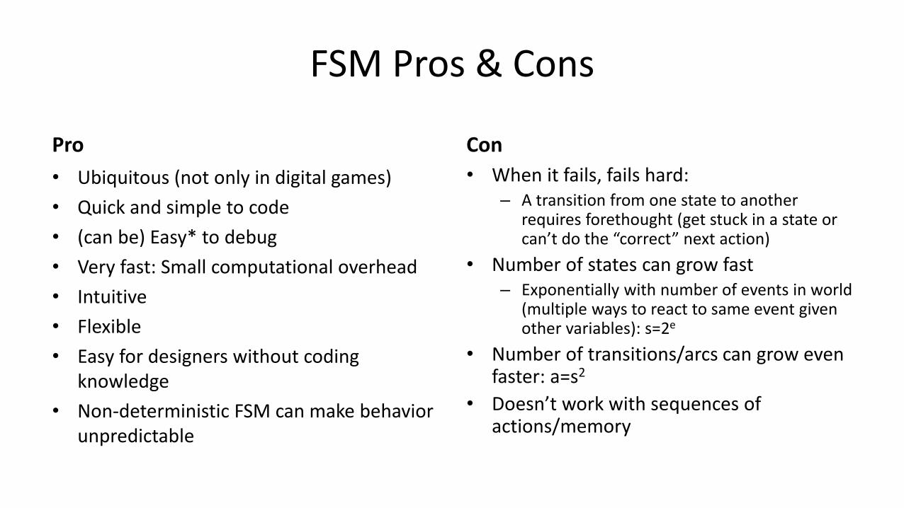
Pro
• Ubiquitous (not only in digital games)
• Quick and simple to code
• (can be) Easy* to debug
• Very fast: Small computational overhead
• Intuitive
• Flexible
• Easy for designers without coding knowledge
• Non-deterministic FSM can make behavior unpredictable
Con
• When it fails, fails hard:– A transition from one state to another
requires forethought (get stuck in a state or can’t do the “correct” next action)
• Number of states can grow fast– Exponentially with number of events in world
(multiple ways to react to same event given other variables): s=2e
• Number of transitions/arcs can grow even faster: a=s2
• Doesn’t work with sequences of actions/memory

More problems with FSM
• Maintainability: – Addition/removal of state requires change of conditions of all other states
that have transition to the new or old one. Susceptible to errors
• Scalability: – FSMs with many states lose readability, becoming rats nest.
• Reusability: – Coupling between states is strong; often impossible to use the same
behavior in multiple projects
• Parallelism:– With a FSM, how do you run two different states at once?
4

Decision Making: (Decision & Behavior) Trees
2019-09-30
M&F Ch 5.2

Decision Trees
M&F 5.3

Decision Trees
• Fast, simple, easily implemented, easy to grok (simple ones)• Modular & easy to create• Simplest decision making technique• Used extensively to control
– Characters– In-game decision making (eg animation); complex strategic and tactical AI
• Can be learned (rare in games) – Learned tree still easy to grok: rules have straightforward interpretation– Can be robust in the presence of errors, missing data, and large numbers of
attributes– Do not require long training times
• w/out learning, it’s essentially a GUI (or fancy structure) for conditionals
8

D-Tree Structure
• Dtree made of connected decision points
– root == starting decision
– leaves == actions
• For each decision, one of 2+ options is selected
• Typically use global game state
9
Decisions
• Can be of multiple types
– Boolean
– Enumeration
– Numeric range
– etc.
• No explicit AND or OR, but representable
– Tree structure represents combinations
10

AND / OR in D-Tree
11Can these be translated into rules? If so, how?

D-Tree Decisions
• No explicit AND or OR, but representable– A AND B: serial TRUE decisions:
• A?->TRUE->B?->TRUE
– A OR B: TRUE if either of:• A TRUE (and B TRUE or FALSE)
• A ?FALSE->B? TRUE
– Tree structure represents combinations
– Lack of compound Boolean sentences is more a convention, as granularity of decisions has benefits for automated restructuring tree later
12
Enemy Visible OR Audible?…or…Enemy NOT Visible AND Audible?

Decision Complexity and Efficiency
• Tree structure affords shared condition evaluation
– Number of decisions in tree usually much smaller than number of decisions in tree
– E.g. 15 different decisions w/ 16 actions, but only 4 considered
• This insight exploited by RETE (later)
• Must tree be binary?
13M&F 5.6

Branching
• N-ary trees
– Usually ends up as if/then statements
– Can be faster if using enums w/ array access
– Speedup often marginal & not worth the effort
• Binary trees
– Easier to optimize
– ML techniques typically require binary trees
– Can be a graph, so long as it’s a DAG
M&F Figs 5.7, 5.8 14
Knowledge Representation
• Typically work directly w/ primitive types• Requires no translation of knowledge
– Access game state directly– Since whole tree isn’t evaluated, expensive to query knowledge can be lazy/on-demand for performance improvement (consider in comparison to rule based system)
– Can cause HARD-TO-FIND bugs• Rare decisions when do pop up, weird effects• Structure of game-state changes breaks things
– Cons avoidable w/ careful world interface• See Millington CH 10
15

Tree Balancing
• More balanced faster (theory)– Balance ~= same number of leaves on each
branch– O(N) vs O(Log2 N)
• Short path to likely action faster (practice)– O(1)– Defer time consuming decisions ‘til last
• Performance tuning– Dark art – since fast anyway, rarely important– Balance, but keep common paths short &
bury long decisionsM&F Fig 5.9
16

See M Ch 5.2
class DecisionTreeNode:def makeDecision() #recursively walk tree
class Action: def makeDecision():
return this
class FloatDecision(Decision):minValuemaxValuedef getBranch():
if max >= test >= min:return trueNode
else:return falseNode
class Decision(DecisionTreeNode):trueNodefalseNodetestValuedef getBranch()def makeDecision() :
branch = getBranch() #runs testreturn branch.makeDecision() #recursive walk
17

Randomness
• Predictable == bad• Can add a random decision node
– random behavior choice adds unpredictability, interest, and variation
• Keep track of decision from last cycle– Random choice made at every frame can
make unstable behavior– Add timeout so behavior can change
• See M 5.2.10 for implementation deets
M&F 5.12
18

D-Trees VS FSMs?
• Decision tree: same set of decisions is always used. Any action can be reached through the tree.– Root to leaf every time
• FSM: only transitions from the current state are considered. Not every action can be reached. – FSM update function called (each frame, or based on transition
condition)
– If transition “triggered”, schedule for “fire” the associated actions (onExit, transition action, onEnter
19

Learning Decision Trees
• Real power of D-trees comes from learning
• Problem: Construct a decision tree from examples of inputs and actions
• Sol’n: Quinlan’s “Induction of Decision Trees”– ID3, C4.5, See5
• http://en.wikipedia.org/wiki/ID3_algorithm
– J48 (GPL java implementation)• http://www.opentox.org/dev/documentation/components/j48
• See Weka (GNU GPL)
20

Andrew Ng – The State of AI (December 15, 2017)
• “99% of the economic value created by AI today is through one type of AI: which is learning a mapping A B, or input to output maps”– Falls under category of supervised
learning
• Other types (ordered falloff)– Transfer learning
– Unsupervised learning
– Reinforcement learning
Input Output
Picture Is it you? (0/1)
Loan application Will the applicant repay the loan? (0/1)
Online: (Ad, User) Will you click? (0/1)
Voice input Text transcript
English French
Car: image, radar/lidar Positions of other cars
https://www.youtube.com/watch?v=NKpuX_yzdYs

Learning Decision Trees
• A simple technique whereby the computer learns to predict human decision-making
• Can also be used to learn to classify
– A decision can be thought of as a classification problem
• An object or situation is described as a set of attributes
– Attributes can have discrete or continuous values
• Predict an outcome (decision or classification)
– Can be discrete (classification) or continuous (regression)
– We assume positive (true) or negative (false)
22
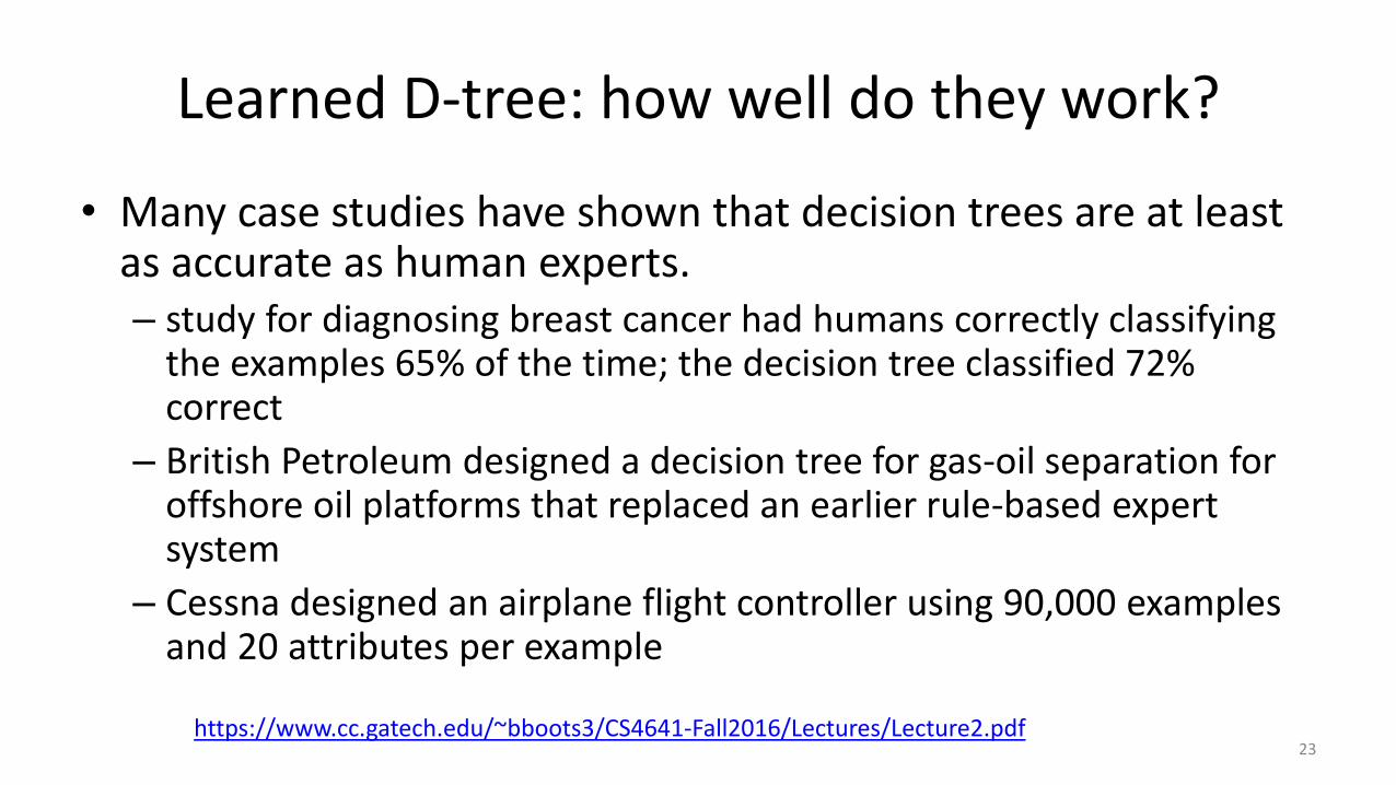
Learned D-tree: how well do they work?
• Many case studies have shown that decision trees are at least as accurate as human experts. – study for diagnosing breast cancer had humans correctly classifying
the examples 65% of the time; the decision tree classified 72% correct
– British Petroleum designed a decision tree for gas-oil separation for offshore oil platforms that replaced an earlier rule-based expert system
– Cessna designed an airplane flight controller using 90,000 examples and 20 attributes per example
23https://www.cc.gatech.edu/~bboots3/CS4641-Fall2016/Lectures/Lecture2.pdf
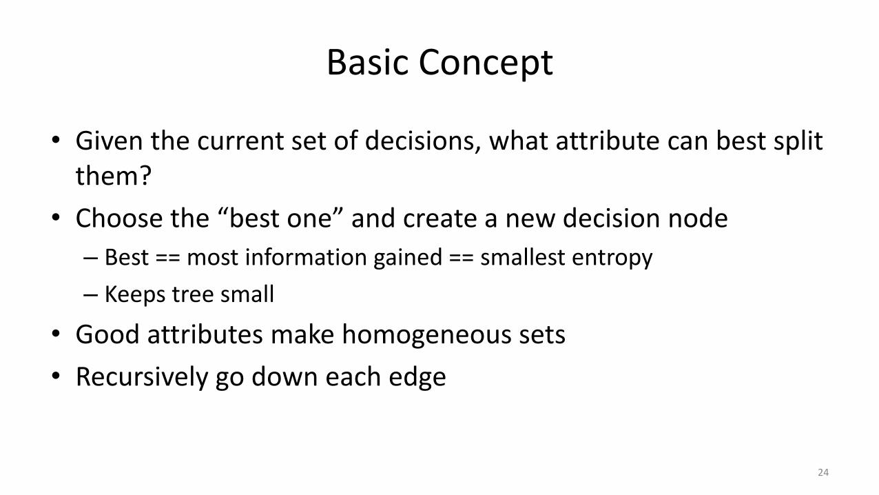
Basic Concept
• Given the current set of decisions, what attribute can best split them?
• Choose the “best one” and create a new decision node
– Best == most information gained == smallest entropy
– Keeps tree small
• Good attributes make homogeneous sets
• Recursively go down each edge
24

ExampleExample Attributes Target
WaitAlt Bar Fri Hun Pat Price Rain Res Type Est
X1 T F F T Some $$$ F T French 0-10 T
X2 T F F T Full $ F F Thai 30-60 F
X3 F T F F Some $ F F Burger 0-10 T
X4 T F T T Full $ F F Thai 10-30 T
X5 T F T F Full $$$ F T French >60 F
X6 F T F T Some $$ T T Italian 0-10 T
X7 F T F F None $ T F Burger 0-10 F
X8 F F F T Some $$ T T Thai 0-10 T
X9 F T T F Full $ T F Burger >60 F
X10 T T T T Full $$$ F T Italian 10-30 F
X11 F F F F None $ F F Thai 0-10 F
X12 T T T T Full $ F F Burger 10-60 T25

Choosing an Attribute
• Idea: A good attribute splits the examples into subsets that are (ideally) “all positive” or “all negative”
• Patrons? is a better choice
26

Attack?
• Attributes:– Bypass? Can be bypassed
– Loot? Has valuable items/treasure
– Achievement? Will unlock an achievement if you win
– On Quest? You are on a quest
– Experience. How much experience points you get
– Environment. How favorable is the terrain?
– Mini-boss? Is this a mini-boss, preventing further progress?
– Element. The elemental properties (earth, air, fire, water)
– Estimated Time. How long will this combat take (quick, short, long, very long)?
– Team size. How many monsters in the team (none, small, large)?
27

Team size
Est. Time
Bypass? On quest?
Mini-boss? Achievement?
Loot?
Bypass?
Environment
No Yes
No Yes
Yes
No Yes
No Yes
Yes
Yes
No Yes
SingleFew
Many
Very longLong Short
Quick
F T
F T
F T
F T
F T
F T
F T
Attack?
28

# Bypass? Loot? Achieve.
On quest
Teamsize
Exp. Env. Mini-Boss
Element
Est. Time
Attack?
1 T F F T few Lot Bad T water quick Y
2 T F F T many Little Bad F air long N
3 F T F F few Little Bad F earth quick Y
4 T F T T many Little Bad F air med Y
5 T F T F many Lot Bad T water v. long N
6 F T F T few Med Good T fire quick Y
7 F T F F single Little Good F earth quick N
8 F F F T few Med Good T air quick Y
9 F T T F many Little Good F earth v. long N
10 T T T T many Lot Bad T fire med N
11 F F F F single Little Bad F air quick N
12 T T T T many Little Bad F earth long Y
29

Pos: 1 3 4 6 8 12Neg: 2 5 7 9 10 11
Element
Pos: 1Neg: 5
Pos: 6Neg: 10
Pos: 4 8Neg: 2 11
Pos: 3 12Neg: 7 8
water
fire air
earth
# Bypass? Loot? Achieve.
On quest
Teamsize
Exp. Env. Mini-Boss
Element
Est. Time
Attack?
1 T F F T few Lot Bad T water quick Y
2 T F F T many Little Bad F air long N
3 F T F F few Little Bad F earth quick Y
4 T F T T many Little Bad F air med Y
5 T F T F many Lot Bad T water v. long N
6 F T F T few Med Good T fire quick Y
7 F T F F single Little Good F earth quick N
8 F F F T few Med Good T air quick Y
9 F T T F many Little Good F earth v. long N
10 T T T T many Lot Bad T fire med N
11 F F F F single Little Bad F air quick N
12 T T T T many Little Bad F earth long Y
30
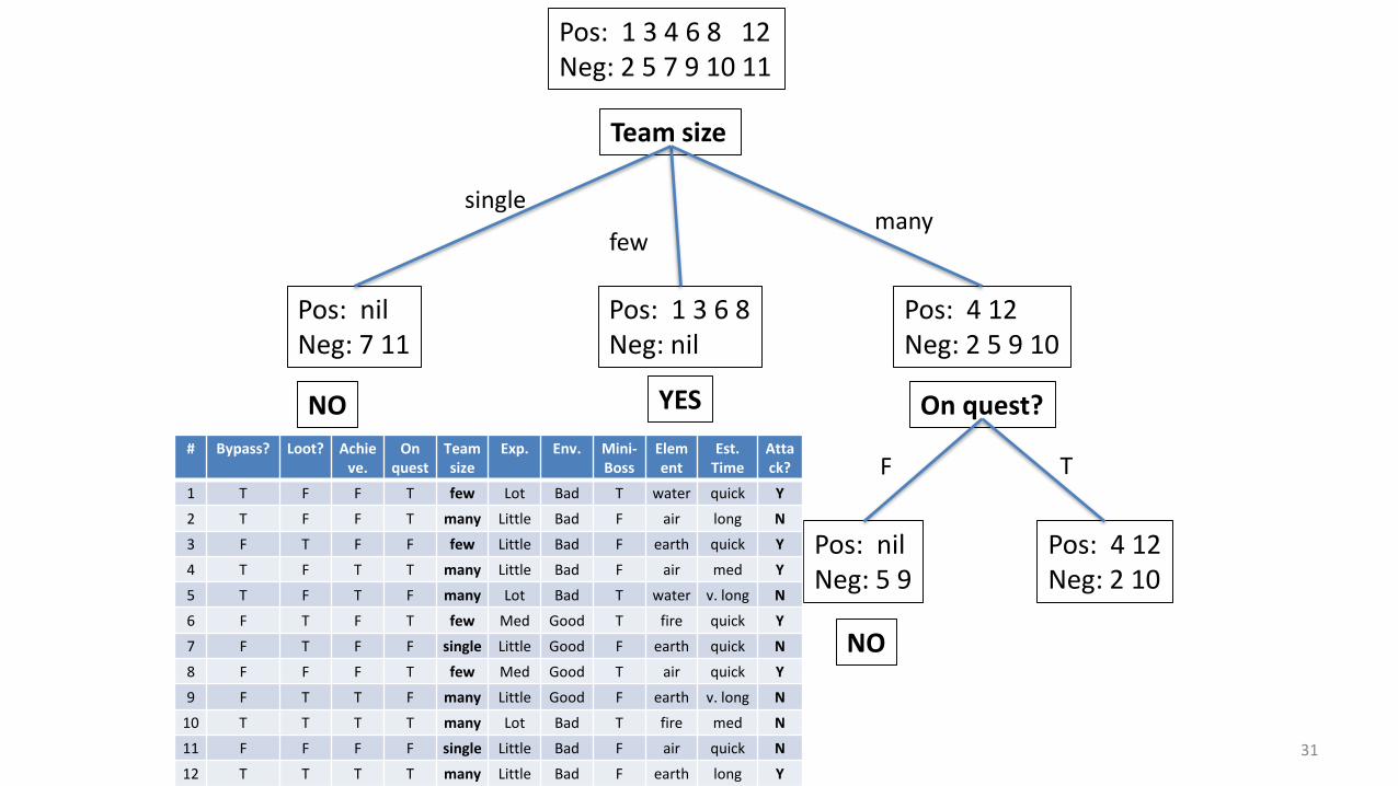
Pos: 1 3 4 6 8 12Neg: 2 5 7 9 10 11
Team size
Pos: nilNeg: 7 11
Pos: 1 3 6 8Neg: nil
Pos: 4 12Neg: 2 5 9 10
single
fewmany
On quest?
Pos: nilNeg: 5 9
Pos: 4 12Neg: 2 10
TF
NO YES
NO
# Bypass? Loot? Achieve.
On quest
Teamsize
Exp. Env. Mini-Boss
Element
Est. Time
Attack?
1 T F F T few Lot Bad T water quick Y
2 T F F T many Little Bad F air long N
3 F T F F few Little Bad F earth quick Y
4 T F T T many Little Bad F air med Y
5 T F T F many Lot Bad T water v. long N
6 F T F T few Med Good T fire quick Y
7 F T F F single Little Good F earth quick N
8 F F F T few Med Good T air quick Y
9 F T T F many Little Good F earth v. long N
10 T T T T many Lot Bad T fire med N
11 F F F F single Little Bad F air quick N
12 T T T T many Little Bad F earth long Y
31

• Learned from the 12 examples
• Why doesn’t it look like the previous tree?
– Not enough examples
– No reason to use environment or mini-boss
– Hasn’t seen all cases
• Learning is only as good as your training data
• Supervised learning
– Training set
– Test set
Team size
On quest?No Yes
SingleFew Many
Element
NoYes
water
fire
Yes
earth
Achievement?
air
No
T F
No Yes
F T
32
Which attribute to choose?
• The one that gives you the most information (aka the most diagnostic)
• Information theory
– Answers the question: how much information does something contain?
– Ask a question
– Answer is information
– Amount of information depends on how much you already knew (information gain)
• Example: flipping a coin
33

Entropy
• Measure of information in set of examples
– That is, amount of agreement between examples
– All examples are the same, E = 0
– Even distributed and different, E = 1
• If there are n possible answers, v1…vn and vi has probability P(vi) of being the right answer, then the amount of information is:
H P(v1),...,P(vn )( ) = - P(vi )log2 P(vi )i=1
n
å34

• For a training set:p = # of positive examples
n = # of negative examples
• For our attack behavior– p = n = 6
– H() = 1
– Would not be 1 if training set weren’t 50/50 yes/no, but the point is to arrange attributes to increase gain (decrease entropy)
Hp
p+n,n
p+n
æ
èç
ö
ø÷ = -
p
p+nlog2
p
p+n-n
p+nlog2
n
p+n
Probability ofa positive example
Probability ofa negative example
Pos: 1 3 4 6 8 12Neg: 2 5 7 9 10 11
35

Measuring attributes• Remainer(A) is amount of entropy remaining after
applying an attribute– If I use attribute A next, how much less entropy will I have?
– Use this to compare attributes
pi +ni
p+nH
pi
pi +ni,ni
pi +ni
æ
èç
ö
ø÷
i=1
v
åRemainder(A) =
Different answers
attribute
Total answers
Instances of the attribute
Positive examplesfor this answer to A
Negative examplesfor this answer to A
Examples classified by A
36

2
12I
1
2,1
2
æ
è ç
ö
ø ÷ +
2
12I
1
2,1
2
æ
è ç
ö
ø ÷ +
4
12I
2
4,2
4
æ
è ç
ö
ø ÷ +
4
12I
2
4,2
4
æ
è ç
ö
ø ÷
Pos: 1 3 4 6 8 12Neg: 2 5 7 9 10 11
Element
Pos: 1Neg: 5
Pos: 6Neg: 10
Pos: 4 8Neg: 2 11
Pos: 3 12Neg: 7 8
water
fire air
earth
Remainder(element) =
water fire air earth
= 1 bit
37

Pos: 1 3 4 6 8 12Neg: 2 5 7 9 10 11
Team size
Pos: nilNeg: 7 11
Pos: 1 3 6 8Neg: nil
Pos: 4 12Neg: 2 5 9 10
single
fewmany
2
12I
0
2,2
2
æ
è ç
ö
ø ÷ +
4
12I
4
4,0
4
æ
è ç
ö
ø ÷ +
6
12I
2
6,4
6
æ
è ç
ö
ø ÷ Remainder(teamsize) =
single few many
≈ 0.459 bit
38

• Not done yet
• Need to measure information gained by an attribute
• Pick the biggest
• Example:– Gain(element) = H(½,½) –
– Gain(teamsize) = H(½,½) –
Hp
p+n,n
p+n
æ
èç
ö
ø÷Gain(A) = - remainder(A)
2
12H
1
2,1
2
æ
èç
ö
ø÷+
2
12H
1
2,1
2
æ
èç
ö
ø÷+
4
12H
2
4,2
4
æ
èç
ö
ø÷+
4
12H
2
4,2
4
æ
èç
ö
ø÷
æ
èç
ö
ø÷
2
12H
0
2,2
2
æ
èç
ö
ø÷+
4
12H
4
4,0
4
æ
èç
ö
ø÷+
6
12H
2
6,4
6
æ
èç
ö
ø÷
æ
èç
ö
ø÷
= 0 bits
≈ 0.541 bits
39

H2
12,
4
12
æ
èç
ö
ø÷-
2
12H
0
2,2
2
æ
èç
ö
ø÷+
4
12H
2
4,2
4
æ
èç
ö
ø÷
é
ëê
ù
ûúGain(quest) =
= 0.959 – [ 0 + (4/12)(1)]
≈ 0.626 bits
Pos: 1 3 4 6 8 12Neg: 2 5 7 9 10 11
Team size
Pos: 4 12Neg: 2 5 9 10
Many
On Quest
Pos: nilNeg: 5 9
Pos: 4 12Neg: 2 10
TF
no yes
teamsize=many, onquest=F
teamsize=many, onquest=T
40

Decision-tree-learning (examples, attributes, default)
IF examples is empty THEN RETURN default
ELSE IF all examples have same classification THEN RETURN classification
ELSE IF attributes is empty RETURN majority-value(examples)
ELSE
best = choose(attributes, example)
tree = new decision tree with best as root
m = majority-value(examples)
FOREACH answer vi of best DO
examplesi = {elements of examples with best=vi}
subtreei = decision-tree-learning(examplesi, attributes-{best}, m)
add a branch to tree based on vi and subtreei
RETURN tree
Where gain happens
41
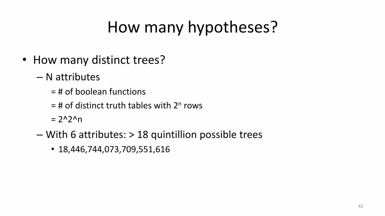
How many hypotheses?
• How many distinct trees?
– N attributes
= # of boolean functions
= # of distinct truth tables with 2n rows
= 2^2^n
– With 6 attributes: > 18 quintillion possible trees
• 18,446,744,073,709,551,616
42

How do we assess?
• How do we know hypothesis ≈ true decision function?• A learning algorithm is good if it produces hypotheses that do a good job of
predicting decisions/classifications from unseen examples1. Collect a large set of examples (with answers)2. Divide into training set and test set3. Use training set to produce hypothesis h4. Apply h to test set (w/o answers)
– Measure % examples that are correctly classified
5. Repeat 2-4 for different sizes of training sets, randomly selecting examples for training and test– Vary size of training set m– Vary which m examples are training
43

• Plot a learning curve– % correct on test set, as a function of training set size
• As training set grows, prediction quality should increase– Called a “happy graph”
– There is a pattern in the data AND the algorithm is picking it up!
44
Noise
• Suppose 2 or more examples with same description (Same assignment of attributes) have different answers
• Examples: on two identical* situations, I do two different things
• You can’t have a consistent hypothesis (it must contradict at least one example)
• Report majority classification or report probability
45

Overfitting
• Learn a hypothesis that is consistent using irrelevant attributes– Coincidental circumstances result in spurious distinctions among examples– Why does this happen?
• You gave a bunch of attributes because you didn’t know what would be important• If you knew which attributes were important, you might not have had to do learning in the
first place
• Example: Day, month, or color of die in predicting a die roll– As long as no two examples are identical, we can find an exact hypothesis– Should be random 1-6, but if I roll once every day and each day results in a
different number, the learning algorithm will conclude that day determines the roll
• Applies to all learning algorithms
46

Black and White
47http://www.ign.com/games/black-and-white
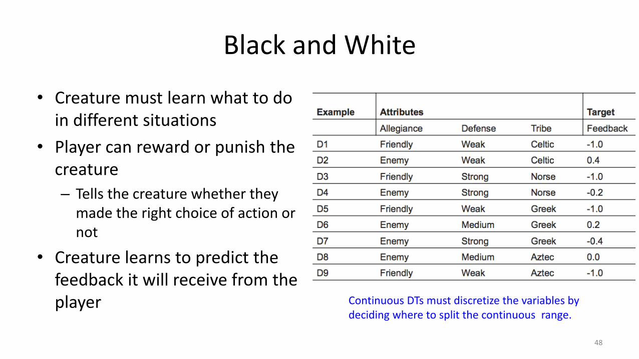
Black and White
• Creature must learn what to do in different situations
• Player can reward or punish the creature
– Tells the creature whether they made the right choice of action or not
• Creature learns to predict the feedback it will receive from the player
48
Continuous DTs must discretize the variables by deciding where to split the continuous range.

No Free Lunch
• ID3– Must discretize continuous attributes
– Offline only (online = adjust to new examples)
– Too inefficient with many examples
• Incremental methods (C4.5, See5, ITT, etc)– Starts with a d-tree
– Each node holds examples that reach that node
– Any node can update self given new example
– Can be unstable (new trees every cycle; rare in practice)
49

But first…
• “What Makes Good AI – Game Maker’s Toolkit”
– https://www.youtube.com/watch?v=9bbhJi0NBkk&t=0s
– https://www.patreon.com/GameMakersToolkit
– React/adapt to the player – no learning required (authoring is)
– Communicate what you’re thinking
– Illusion of intelligence; more health & aggression can be a proxy for smarts
– Predictability is (usually) a good thing
• Too much NPC stupidity can ruin an otherwise good game
50

Next Class
• More decision making!
– Behavior trees
– Production / Rule Based systems
– Fuzzy logic + probability
– Planning
51
BEHAVIOR TREES (M CH. 5.4)
52

Next Class
• More decision making!
– Behavior trees
– Production / Rule Based systems
– Fuzzy logic + probability
– Planning
53
Top Related