


Languages
Pages
Legal

Established and supported under
the Australian Government’s
Cooperative Research Centres
Program
Determining the variability in eating quality of Australian fresh pork
3B-101
Report prepared for the Co-operative Research Centre for High Integrity Australian
Pork
By
C.G. Jose1, M. Trezona1, B. Mullan1, K. McNaughton2 and D.N. D’Souza3
1Department of Agriculture and Food Western Australia 3 Baron Hay Court, SOUTH PERTH WA
2South Australian Research and Development Institute
GPO Box 397, ADELAIDE SA 5001
3Australian Pork Limited P.O. Box 4746
KINGSTON ACT 2604
June 2013
i
Executive Summary
Consumer fail rates for eating quality of pork in Australia have been reported to be as high
as 30%. As the Australian pork industry needs to limit these levels to below 10%, strategies
to optimize eating quality need to be implemented by the whole supply chain. The large
fail rates are likely due to variability in carcase characteristics; however, the exact
cause(s) has not been identified. One likely factor is the variation in pH and pH decline
between carcases. The pH and pH decline is primarily driven by the amount of stored
energy in the form of glycogen that the animal has in its muscles at slaughter and this can
be affected by a number of processing technologies. Furthermore, it has been noted that
the ultimate pH (pHu; the pH reached once post mortem metabolism has ceased;
measured at 72 hour post mortem in the current study) of Australian pork has declined to
levels lower than what is considered “normal” (ie. < 5.5). It is not known what impact this
observed decrease in ultimate pH may be having on consumer acceptability and eating
quality. Thus, this study was designed to investigate the effect of a range of pHu (pHu
5.35-5.65), from low (5.35 to 5.5) to normal (5.5.1 to 5.65), on consumer sensory and meat
quality attributes of loin (M longissimus dorsi) muscles sourced from female and entire
male pigs from two Australian supply chains.
This study was a 2 (supply chains) x 2 (sex; female, entire male) x pHu category (low 5.35-
5.5; normal 5.5-5.65) factorial study. The design allowed for the analysis of pHu as a
covariate due to the range of pHu of muscles selected for use in the study. A total of 160
loins (80 per supply chain) from entire male and female carcases were selected on the
basis of pHu. Loins were also tested for colour and drip loss as part of the selection
procedure and any outliers were excluded. Four steaks from each loin were cut and aged
for 7 days before being frozen and sent to SARDI for sensory analysis. A total of 160
consumers were used for the study, with 640 total evaluations of sensory meat quality
being collected. Objective meat quality measures of colour, drip loss, cook loss, shear
force and intramuscular fat (IMF) were also measured.
The key findings from this experiment were:
Consumers preferred loin steaks with a higher pHu, favoring samples that were
towards the higher end of the pH range. This preference increased linearly across
the range of pHu sampled. The largest effect of pHu was observed for sensory
tenderness in female carcases, with a 22% improvement in tenderness scores across
the pHu range.
Consumers discriminated against samples with poor objective meat quality
measurements, particularly, shear force. Shear force correlated highly with
tenderness thus highlighting the importance of tenderness in consumer acceptance.
Strong correlations were also found between shear force and quality grade and re-
purchase intention
Shear force, drip loss, cook loss and L value (muscle lightness) were all positively
influenced by pHu as well as pH measured at 24 hours post mortem (pH24). The
fact that pH24 correlated with these measures reinforces the importance of the
rate of pH decline on meat quality.
Glycogen concentration at slaughter correlated strongly with pHu, however lactate
concentration did not. This suggests that glycogen concentration at slaughter is a
driver of pHu and pH decline and strategies to optimize muscle glycogen
concentrations should be further considered

ii
Drip loss percentage from loin differed between supply chains. This may reflect
differences in processing factors influencing early post mortem decline and/ or
different rates of chilling.
The outcomes from this experiment indicate that strategies need to be developed to
optimize the rate and extent of pH decline to improve consumer acceptability and reduce
the variability in pork eating quality.
iii
Table of Contents
Executive Summary .................................................................................... i
1. Introduction ....................................................................................... 1
2. Methodology ...................................................................................... 2
2.1. Experimental design .........................................................................2
2.2. Supply chain information ...................................................................2
2.3. Sample collection ............................................................................2
2.4. Objective measures .........................................................................3
2.5. Sensory measurements ......................................................................4
2.6. Sensory Evaluation...........................................................................4
2.6.1 Consumer Recruitment ...................................................................4
2.6.2 Allocation of Frozen Samples into Sensory Sessions .................................5
2.6.3 Thawing and Preparation Protocols ....................................................5
2.6.4 Grilling Protocol ...........................................................................5
2.6.5 Presentation Protocol ....................................................................6
2.6.6 Serving of Samples to Consumers .......................................................6
2.6.7 Consumer Evaluation .....................................................................7
2.7. Data analysis .................................................................................8
3. Outcomes .......................................................................................... 9
3.1. Objective and carcase measurements ....................................................9
3.2. Sensory measurements .................................................................... 16
3.2.1 Demographics ............................................................................ 16
3.2.2 Sensory results .......................................................................... 19
3.2.3 Sensory fail and premium rates ....................................................... 24
3.3. pH analysis .................................................................................. 27
3.3.1 pH sensory ............................................................................... 27
3.3.2 pH objective ............................................................................. 31
3.4. Sensory objective .......................................................................... 34
3.5. Glycogen utilization ....................................................................... 37
3.6. Intramuscular fat content ................................................................ 40
4. Application of Research ....................................................................... 41
4.1. Sensory and objective eating quality in relation to ultimate pH .................. 41

iv
4.2. Effect of Supply chain and sex on sensory and eating quality ...................... 42
4.3. Management of pH and meat quality ................................................... 42
5. Conclusion ........................................................................................ 44
6. Limitations/Risks ................................................................................ 44
7. Recommendations ............................................. Error! Bookmark not defined.
7.1. Implications ................................................................................. 45
7.2. Recommendations ......................................................................... 46
8. References ....................................................................................... 47
1
1. Introduction
To ensure the maintenance and growth of domestic pork consumption, and growth of the
export market for premium pork products, pork consumers must be confident they will have
a positive eating quality experience when purchasing fresh pork. Thus, the availability of
pork of variable eating quality needs to be minimized or completely eliminated from the
supply chain . To accomplish this, it is important for the industry to be aware of the current
fail rate levels and have an understanding of the basis of poor eating quality.
It is well documented that both production and processing factors contribute to pork quality
and therefore subsequent eating quality. Production factors include genotype, sex,
production system, nutrition and season, while processing factors include carcase chilling
regime, moisture infusion and aging. Many of these factors have the ability to manipulate
pH, which in turn can have a massive detrimental effect on meat quality. Pork with an
increased ultimate pH (pHu; when a decline in pH has ceased; measured at 72 hours post
mortem) of 5.8-6.0 tends to result in a higher rating for consumer overall liking with
interactions between cooking temperature also identified (Bryhni et al., 2003). Pork with a
lower ultimate pH seems to be correlated with a negative sour/acidic flavour (Aaslyng et
al., 2007; Myers et al., 2009) as well as decreased juiciness and tenderness (Lonergan et al.,
2007), thus effecting the overall liking of the product.
Previous work carried to assess the benchmark of pork eating quality across Australia,
identified a trend towards lower pHu meat, without being classed as pale soft and exudative
(PSE) and separate to the RN- gene. The mean pHu from 8 farms across Australia ranged
from pH 5.43 to 5.00 - levels that would traditionally fit well within typical PSE limits. There
is also evidence that low pH pork was present in both Western Australia and Victoria
(D’Souza and Moore, 2005). However, this work was performed over a decade ago and the
present industry average pHu is currently unknown. Assuming the ultimate pH of pork across
Australia has shown a trend to be reduced, and not being PSE, a more definitive
understanding of the impact of low pH pork on both sensory and meat quality is required.
This study was conducted to quantify and redefine the inconsistencies in eating quality
occurring in fresh Australian pork. The aim was to determine the current level of variability
in eating quality in Australian fresh pork and identify reasons (consumer generated) why
pork fails to meet consumer eating quality standards. The association of this fail rate in
relation to pH was of particular interest. Profiles of eating quality variability were
developed for two major supply chains identifying differences in genotype and sex. The
effects of different production systems and carcass chilling regimes were not addressed,
however the production system and chilling program for the locations where samples were
collected were noted and variability minimised. Samples analysed in this study were not
moisture infused.
The identification of any inconsistencies will allow interventions to be developed for
different pork production systems. The interventions can then be used as tools to reduce the
incidence of unacceptable product quality. This project will also provide essential
information to assist in building a profile of current consumer expectations of fresh pork in
Australia and provides further data/information to complement the CRC for High Integrity
Australian Pork project 3A, developing predictive models for pork quality. By investigating
the relationship between low ultimate pH and sensory eating quality, potential management
strategies to improve the consistency of pork eating quality are likely to become evident.
2
2. Methodology
2.1. Experimental design
Samples were collected from finisher carcasses from two major Australian supply chains.
Selected carcasses were categorised by sex (entire male or female) and ultimate pH (Low:
5.35-5.5; Normal: 5.5-5.65). There were a total of eight treatments (2 supply chains x 2
sexes x 2 pHu categories) with 20 animals per treatment; a total of 160 animals.
2.2. Supply chain information
The two supply chains differed in geographical location. Carcases sampled came from two
different genotypes and all pigs were commercial crosses (Landrace x Large White x Duroc).
Pigs sourced from Supply Chain 1 (SC1), were housed in ecoshelters and fed five different
diets from weaning to slaughter. Diets were wheat/barley based rations, with lupins
included in grower and finisher rations. The digestible energy content ranged from 15MJ to
13MJ. The farm was located 300km from the abattoir and pigs were transported in loads of
approximately 240.
Pigs from supply chain 2 (SC2) were also housed in straw based ecoshelters and fed a
wheat/barley plus pulse based diet. Pigs were fed seven different diets from weaning to
slaughter and ranged in digestible energy from 16MJ to 13.8MJ. The farm was located 170km
from the abattoir and pigs were transported in loads of 220-230.
Both supply chains used CO2 stunning to anaesthetize pigs prior to exsanguination. For SC1,
hair was removed from the carcase by scalding in water baths at a temperature of 61°C for 5
minutes. Time from stunning to entering the chiller was 35-45 minutes, and the chillers
were set at 0oC. For SC2, hair was removed by steam at a temperature of 60.7-61.7oC and
time from stunning to entering the chiller was also 45 minutes. Chillers were set at 1.5oC.
2.3. Sample collection
Samples were collected across the two supply chains from May to October 2012) over ten
different sampling days (6 days for SC1 and 4 days for SC2). One hundred pigs were tested
for pH at 24 hours per sampling day. Hot carcass weight and P2 backfat depth for selected
carcasses were recorded. About 1 kg of loin muscle (m.longissimus dorsi) was removed from
the right hand side of the carcase and transported to South Perth, Western Australia for
further objective analysis.
At 48 hours post-slaughter, 4 2.5cm thick steaks were cut from each loin piece, vacuum
packaged and labeled individually for sensory analysis, aged for 7 days at 2oC and then
frozen at -20oC. These samples were sent to SARDI, Adelaide for sensory analysis. At the
same time a 40±5g sample (weights recorded) was cut and used to measure drip loss and
intramuscular fat (IMF) content. A final sample of 70±5g (weight recorded) was cut into a
cube and vacuum packaged, aged for 7 days at 4oC and then frozen at -20oC. This sample
was used for shear force and cook loss analysis.
For each loin, muscle pH at both 48 and 72 hours were measured and those samples that
fitted into either of the pHu categories were selected for the experiment. Samples which
3
had PSE characteristics were eliminated from the experiment and drip loss and colour were
also discriminated against (any outliers were removed).
2.4. Objective measures
Muscle pH was determined at 24, 48 and 72 hours post-slaughter in the loin. The pH was
measured using a pH 300 hand-held pH/mV/temperature meter (Eutech instruments,
Singapore) fitted with a temperature and IJ44C intermediate junction pH probe (Ionode,
Tennyson). The pH meter was calibrated on two standards (pH 4.01 and 7.0) as per
manufacturer’s instructions. At 24 hours, the probe was inserted into the loin muscle on the
right side of each carcass between the 3rd and 4th ribs 7.5 cm from the ventral edge of the
split pork carcass (pH24 measurement). At 48 and 72 hours, the pH was measured directly
into the removed piece of loin. The pH at 72 hours was considered the ultimate pH (pHu).
Loin colour was measured at 48 hours post slaughter. Muscle samples were cut and a surface
was exposed to air at room temperature for 10 min. Meat colour was determined using a
Minolta Chromameter Model CR-400 (calibrated on a white tile) set on the L*, a* and b*
system where L* denotes relative lightness (higher L* values = paler meat), a* relative
redness (higher a* values = more red) and b* relative yellowness (higher b* values = more
yellow), using D65 illumination and a 2 standard observer.
Drip loss was determined using a modified method of Honikel (1998). A sample of pork loin
was cut to a 40 g cube, weighed and weight recorded. The sample was then wrapped in a
piece of square netting. The wrapped sample was then suspended in a 200 ml plastic
container and left to stand in a 4C chiller for 24 h, after which it was removed from the
container, gently rolled in paper toweling and reweighed to determine percentage drip loss.
The remaining sample was then frozen at -20oC and used for IMF analysis.
Samples for intramuscular fat measurement were freighted to Silliker Australia, Regents
Park, (Sydney) for analysis using the Ankom method (extraction of crude fat using petroleum
ether).
Samples for WBSF were cooked from frozen state and dependent on internal temperature
treatment, cooked in a water bath preheated to 70°C until an internal temperature of 70°C
was attained. Each sample was suspended from a metal rack and cooked in a water bath.
Samples were then cooled in iced water for 30 minutes. Samples were dried and weighed to
determine cook loss (expressed as a percentage of weight lost due to cooking) and then
stored at 4C for 24 hours. From each sample, five 1 cm2 replicate samples were cut parallel
to the orientation of muscle fibres and WBSF was measured using a Warner Bratzler shear
blade fitted to a Lloyd Texture Analyser (TA-2, United Kingdom).
Analysis of the muscle samples collected were chemically analysed for lactate and residual glycogen content at Murdoch University. The glycogen assay was based on the enzymatic method of Chan & Exton (1976) but excluding the filter paper step, and the lactate assays used the same homogenate. Briefly, 250 mg of frozen LD muscle samples were weighed out into test tubes and kept on ice. Next, 2.5 mL of 30 mM HCl was added to the test tubes and the sample was homogenized for 30 sec using a Polytron (Bosch GGS 27C Professional) and left to settle whilst on ice for 1-2 h. Sample liquid (not foam) was transferred to Eppendorf tubes and frozen at -20 °C until required. The auto-analyser (Olympus AU 400, Olympus Diagnostics, Tokyo, Japan) used for completing the analysis was calibrated using lactate and glucose standards according to the machine manual, then 60 μl of defrosted, vortex spun samples were pipetted into auto-analyser cups and analysed for lactate. Glycogen in each of
4
the remaining homogenate samples was then broken into glucose for analysis in the auto-analyser, by combining 125 μl of homogenate with 125 μl of distilled water and 1 mL of an enzyme and acetate buffer mixture (0.0128 mg amylase, 0.0128 mg amyloglucosidase in 80 mL of pH 4.8, 40 mM acetate buffer (0.41 g sodium acetate, 0.3g glacial acetic acid and distilled water)) and incubating in shaking water bath at 37 °C for 60 min. This mixture was then pipetted in 60 μl aliquots into auto analyser cups and analysed for glucose content to establish the amount of total residual glycogen in the muscle sample (number of moles of glucose reflects the number of moles of glycogen in the sample). Total glycogen was calculated by adding the number of moles of residual glycogen with half the number of moles of lactate (equivalent of two lactate molecules to every one glucose or glycogen) and converting to g per 100 g of muscle sample. This resulted in a value for total glycogen at slaughter, while lactate measures were what was present in the tissue at 72 post slaughter.
2.5. Sensory measurements
The study was designed with three factors (supply chain, sex and pH) with two levels within
each factor giving eight treatments. The levels for each factor were:
Supply Chain: SC1 and SC2
Sex: Entire male and female
pH: low and normal
One primal cut (loin) and one cooking method (grilling as steaks) were evaluated. One loin
primal was obtained from each pig which was cut into four loin steaks of 2.5 cm thickness;
a total of 640 loin steaks. Each loin steak was aged for seven days post-slaughter and
cooked to a 70°C endpoint temperature. Panelists evaluated four loin steaks in each
sensory session, requiring 160 consumers.
2.6. Sensory Evaluation
The consumer panel was designed to determine sensory attributes of aroma, tenderness,
juiciness, flavour and overall liking for each pork loin steak sample assessed. Demographic
information (gender, household size, age, current purchasing, cooking and consumption
habits of fresh pork) was also captured for each consumer along with a quality grade and re-
purchase intention score for each pork sample evaluated.
The consumer sensory sessions were conducted at one central location at the University of
South Australia (UniSA) sensory facilities based at the city centre campus in Adelaide.
2.6.1 Consumer Recruitment
Consumers were recruited by an independent recruitment company (Intuito Market
Research) by emailing their extensive database of consumers willing to participate in taste
testing.
All participants needed to be consumers who had eaten fresh pork (not bacon or ham) in the
past month and aged between 18 and 65 years. Butchers and other people working with
meat production and sales were excluded. Individuals (n=160) were asked to join a panel of
eight consumers for approximately 40 minutes at session times of 10.00 am, 11.30 am,
1 pm, 2.30 pm and 4.00 pm on four pre-determined days from Monday to Thursday in
November 2012.
Potential participants registered with Intuito, either online or over the telephone, and were
contacted by a recruiter to arrange a time that would suit them to attend. Participants who
5
cancelled their appointments were replaced using the database of over 1,000 consumers.
Participants were given an honorarium for their participation in the study and were used
only once.
2.6.2 Allocation of Frozen Samples into Sensory Sessions
The pork loin steak samples, prepared at SC2 by Dr Cameron Jose, were individually vacuum
packed at the SARDI Waite campus, stored in a cool room (4°C) for a seven day ageing
period and then frozen to -18°C. Samples from SC1 were supplied to the SARDI Waite
campus in a frozen format and stored at -18°C until required for the sensory sessions. The
samples were prepared and frozen during the period July – September 2012. Loin steak
samples were sorted into the individual sensory sessions in the product development kitchen
at the SARDI Waite campus.
Copies of a one page session labeling document were prepared in advance for every session
to indicate which loin steaks (n=32) were required for the sessions. The document showed
the session number and a list of the 3 digit codes for each loin steak required along with
details of the supply chain, sex and pH. The 32 loin steaks required for each session were
located using the session labeling document, checked off the list and put into a plastic bag.
Once all samples had been located, the session labeling document was also placed inside the
plastic bag; the bag was sealed and returned to the freezer at SARDI Waite. Once this was
completed, five sessions required for each day were then collated into one carton and
labeled with the session numbers.
2.6.3 Thawing and Preparation Protocols
The carton required for each day of sensory sessions was removed from the -18°C freezer
and placed into the 4°C constant temperature room for 48 hours. Samples were prepared
for the sensory sessions between one and seven hours after removal from the 4°C room.
On each day of the sensory sessions the carton was collected from SARDI Waite campus (at
8 am) and transported to the central testing location at UniSA by car. The carton was
transported in the boot of the car and the journey was approximately 15 minutes. The
sensory sessions were undertaken in November 2012. The average minimum temperature in
Adelaide in November was 15.1°C (Australian Government Bureau of Meteorology, Accessed
12 Feb 2013)}. The samples were not transported under refrigerated conditions due to the
short transport time and low ambient temperature.
On arrival at the test location, the samples were removed from the carton. Samples for
Sessions 2 - 5 were placed on separate shelves in a holding chiller (5°C) and preparation
commenced with samples for Session 1.
On removal from the carton, the 32 individual loin steak samples were checked against the
session labeling document to ensure the session contained the correct samples. The 3 digit
number was used as the primary identification tool. Each sample was identified by its
unique 3 digit number and this ID followed the sample from removal from its vacuum
packaging to presentation to the sensory panelist for evaluation.
2.6.4 Grilling Protocol
The loin steaks were removed from the vacuum packaging, labeled with their 3 digit
number, placed onto a tray and stored at 5°C until required. The temperature of the loin
steaks was 5-7°C before cooking commenced. The four samples to be evaluated by each
6
consumer were in a randomised tasting order so the cooking of samples (n=32) could not be
done to order. The loin steaks were grilled in groups of four loin steaks with eight grilling
batches required for each session.
The grill used for this study was a Silex Grill Model GTTPowersave 10.10-30 (Silex
Elektrogerate GmbH, 22143 Hamburg, Germany). The grilling protocol was that previously
developed and utilised in Pork CRC project 3A-103 to produce grilled steaks cooked to an
end point temperature of 70°C after a two minute resting period. The grilling started
approximately 40 minutes before the start of each session.
For every group of loin steaks grilled, the internal take-off and resting temperature was
measured for one steak cooked to ensure the equipment was functioning as expected and
the required end point temperature of 70°C was achieved. The grilling and resting times
were measured with digital timers.
Once the steaks had been grilled for the required amount of time, they were removed from
the grill and placed next to their ID label on the cutting board for resting. This process was
repeated until all 32 steaks had been cooked for the session. In between each sensory
session the grill was switched off and the plates thoroughly cleaned with hot water and
detergent.
2.6.5 Presentation Protocol
The preparation room was maintained at a temperature of 23°C during the sensory sessions.
In each session, the samples (n=4) evaluated by each consumer (n=8) were in a randomised
tasting order so all samples (n=32) needed to be prepared and ready to serve for the start of
the sample evaluation section of the sensory session; approximately 10 minutes after the
start of the session. The samples could not be prepared to order. Some samples were stored
in the containers for up to 45 minutes prior to consumer evaluation.
To keep the prepared samples warm during the evaluation and prevent moisture loss they
were stored in sealed and labelled glass Pyrex containers (World Kitchen, Rosemont, Illinois,
USA) on top of heated warming plates (n=4) from Cuisinart Model CWT-240A (Cuisinart
Australia, 24, Salisbury Road, Asquith, NSW, Aus.). At the start of the day, the warming
plates were preheated to the 65°C setting and the Pyrex containers (n=16) placed on top. A
duplicate set of Pyrex containers was available so these could be placed on the warming
trays to pre-heat for the next sensory session whilst the soiled ones were cleaned.
After two minutes resting on the cutting board, four steaks (grilled at the same time) were
trimmed on all four sides to remove the fat and edges and the centre pieces used for
consumer evaluation. These were transferred with their labels to sealed Pyrex holding
containers. Two steak pieces were placed at each end of an individual container. This
process was repeated for the 32 steaks required for each sensory session.
2.6.6 Serving of Samples to Consumers
A one page serving order document was prepared for each of the 160 consumers in the
study. This document contained the order in which the four samples were to be tasted
(identified by order, sample description and 3 digit identification number) by each panelist
in each session. Before the start of each session, the page corresponding to the correct
session and panelist was secured above the booth for each consumer in the preparation
room. The four sample plates were also pre-labeled with the 3 digit sample numbers and
stacked in the correct tasting order by the booth.
7
The consumers were instructed to switch on a light in their booth once they were ready to
evaluate a sample of pork. This action illuminated a duplicate light in the preparation room
which served as a signal to commence the serving process to that consumer. Two people
undertook the serving of samples in a sensory session; one person responsible for serving
Panelists 1-4 and the other for Panelists 5-8.
When a consumer was ready for a sample and the light was illuminated, the server would
identify the panelist and sample number required. They would:
1. collect pre-labeled sample plate from beside the tasting booth;
2. locate the correct sample in the Pyrex container;
3. undertake a number identification check between plate and Pyrex container;
4. place sample onto plate;
5. open the serving hatch and present the sample to the consumer;
6. switch off the light beside the tasting booth; and
7. cross out the sample ID number on the serving order document.
This process was repeated for all four samples and the protocol followed for all sensory
sessions. The serving operation was completed in approximately 20 to 25 minutes per
session.
2.6.7 Consumer Evaluation
In each sensory session (n=20), eight consumers evaluated four pork samples (32 tastings).
The eight consumers registered at the start of each session were given a short briefing on
the sensory evaluation process and then taken to the sensory evaluation room and placed in
the eight individual tasting booths to start the session. Panelists recorded assessments by
touch screen through the use of a computerised sensory evaluation program, Compusense
Five version 5.2 (6/9 Southgate Drive, Guelph, Ontario, Canada).
The session commenced with consumers answering a number of questions presented on the
screen to capture individual demographic information which included: gender, household
size, age, current purchasing, cooking and consumption habits of fresh pork. Consumers
were then presented with each pork sample for evaluation on a numbered plastic plate as
per the serving protocol described above. They were first asked to enter the 3 digit
identification number for the sample, smell it and rate the sample for aroma. They were
then asked to eat most of the sample before scoring for tenderness, juiciness, flavour and
overall liking.
Consumers assessed the eating quality attributes of the pork samples using a continuous line
scale as per Australian Standard for Sensory Analysis (AS 2542, 2007). This method provided
panelists with an opportunity to express small differences in judgment as they marked the
line in the position corresponding to perceived intensity for that attribute. Although
potentially a more difficult task for the consumer than using a category scale, the line scale
permits unlimited fineness of differentiation among consumer assessments. To ensure that
the scale was easily understood by panelists, word anchors were carefully selected for each
attribute and prior to the evaluation of pork samples, consumers completed a number of
line scale practice assessments.
The continuous line scales used for the five quality attributes were anchored at each end
with words with left hand side equivalent to 0 and right hand side equivalent to 100.
Numerical intensity values were not shown to the consumers:
8
1. Aroma liking: Dislike extremely to Like extremely.
2. Tenderness: Not tender to Very tender
3. Juiciness: Not juicy to Very juicy
4. Flavour liking: Dislike extremely to Like extremely
5. Overall liking: Dislike extremely to Like extremely
Each consumer also graded the samples for quality into one of the following categories:
1. Unsatisfactory (this was terrible, I did not enjoy it all)
2. Below average (this was not nice, I did not enjoy it)
3. Average (this pork was nice, I somewhat enjoyed it)
4. Above average (this pork was really nice, I enjoyed it)
5. Excellent (this pork was excellent, I really enjoyed it)
Each sample was also rated for repurchase intention into one of the following categories:
1. I definitely would not buy it
2. I would probably not buy it
3. I might buy it
4. I would probably buy it
5. I would definitely buy it
Consumer assessment progress was monitored remotely on the laptop running the
computerised program and assistance was provided when required. Consumers could not
move onto the next question or assessment until the previous answer or assessment was
completed. The session was completed once all consumers had assessed and rated their
seven samples.
2.7. Data analysis
The software package SAS® was used for all statistical analyses (SAS Institute, 2001). Sensory
data was analysed in a two-step process. Each sample was scored by 4 different consumers
and thus had 4 scores per question. The means of these scores for a sample were adjusted
for by the consumer, outputted so there is one score per sample, and included in the master
data set.
Data were analysed using a linear mixed effects model, using sex, supply chain and pHu
category as fixed effects, with day of sampling within supply chain as the random term. First
order interactions as well as all two way and three way interactions were tested. In a
separate analysis, pHu and pH24 were used as covariates, with sex and supply chain as fixed
effects and day of sampling within supply chain as the random term. Linearity and curve-
linearity were tested for pHu and pH24 as well as all two and three way interactions.
Interactions with non-significant (P>0.05) interactions were removed in a step wise
regression process. A similar model was used to test interactions of objective measures and
sensory scores.
9
3. Outcomes
3.1. Objective and carcase measurements
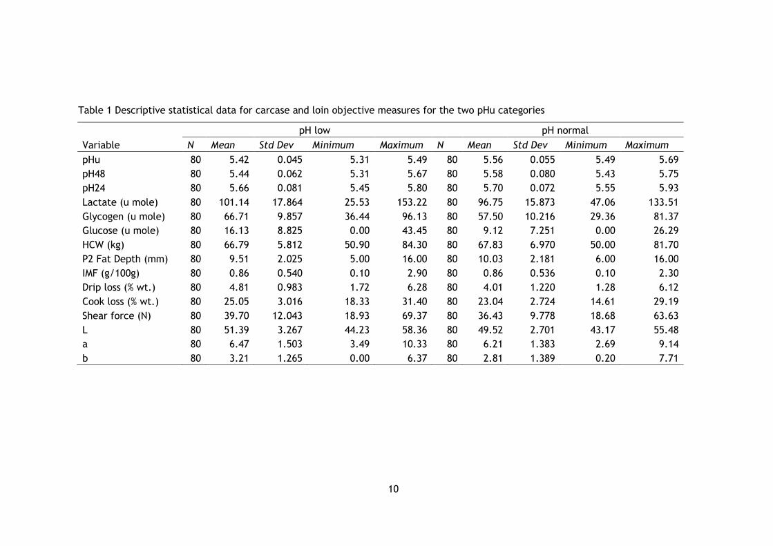
The raw means data for pH category are described in Table 1. Briefly, the low pH category
ranged from pHu 5.31-5.49 with a mean of 5.42 ± 0.005, while the normal category ranged
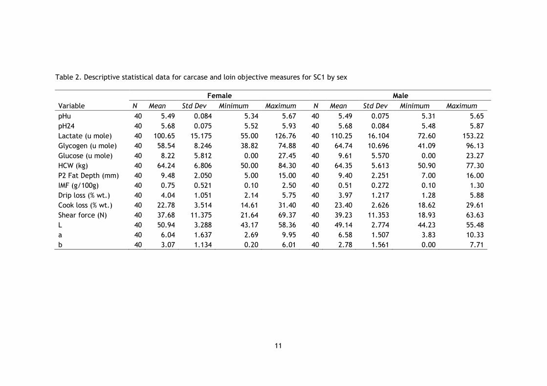
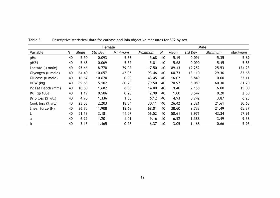
from 5.49-5.69 with a mean of 5.56 ± 0.006. The raw means data for SC1 by sex is shown in
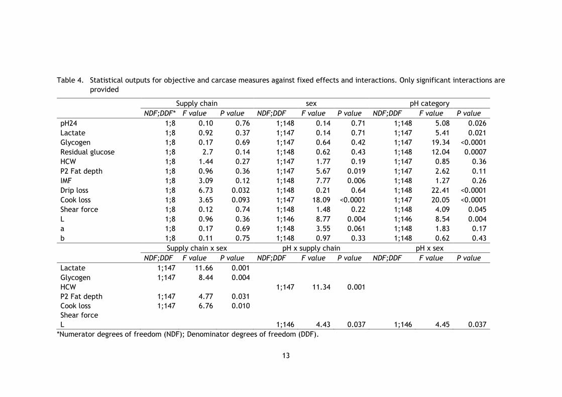
Table 2 and SC2 by sex in Table 3. The statistical outputs for the main fixed effects (sex,
supply chain and pHu category) and treatment interactions are described in Table 4. The
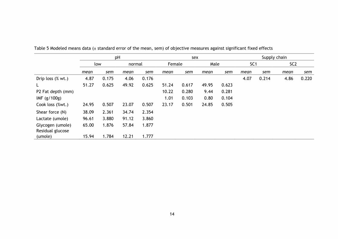
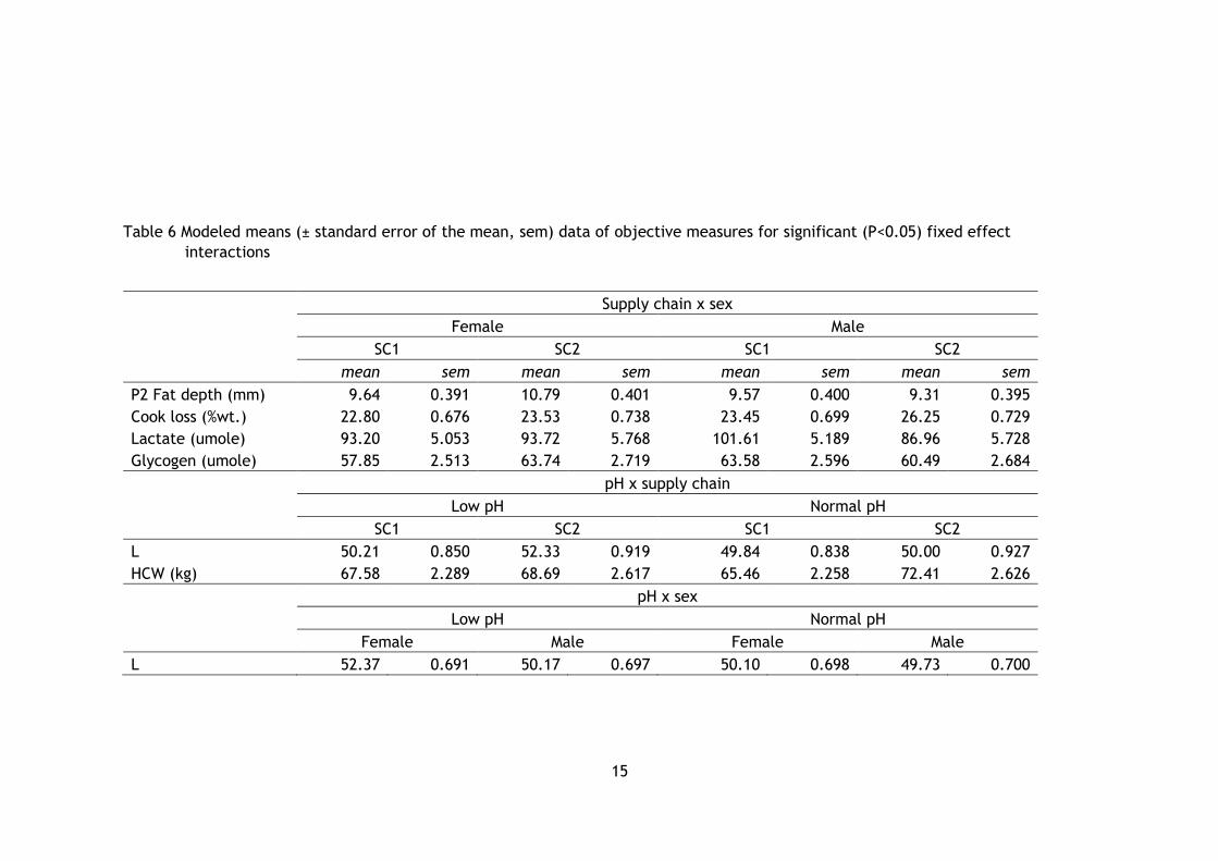
modeled mean values for statistically significant outputs are described in Tables 5 and 6.
Ultimate lactate, glycogen at slaughter and residual glucose levels were higher (P<0.05) in
loins with a low pHu. Furthermore, lactate levels were higher in males from SC1 across all
pHu levels. Lactate levels in males from SC2 were lower (P<0.001), whilst females from
both supply chains had the similar lactate levels. Glycogen levels at slaughter were lowest
in SC1 females across all pHu levels (P<0.01). These interactions are possibly due to the
biased selection for pHu when collecting samples. The mean pH24 differed between pHu
categories with the “low” pHu group being about 0.03 pH units lower than the “normal” pHu
group at 24 hours post mortem (P<0.05).
There was no difference in hot carcase weight (HCW) between any main fixed effects,
although normal pHu carcases were heavier from SC2 (P<0.001). Female carcases from SC2
had a higher P2 fat depth measurement (P<0.05), while females had more IMF than males
(P<0.01), however this level of IMF is still considered low.
Percentage drip loss, cook loss and shear force were all higher in the lower pHu treatment
(P<0.05). SC2 samples lost about 0.8% more weight through drip loss in 24 hours than SC1
samples (P<0.05). There was a significant effect of sex on cook loss, which was driven by an
increased loss in males from SC2 worth about 3% in weight lost (P<0.01).
An effect of sex and pH category existed for L value; generally males samples with a normal
pH were slightly darker (P<0.01). L value differed further with interactions on pH by supply
chain and pH by sex. It seemed that low pH females, and samples from SC2 with low pH
were the lightest (P<0.05) in these interactions. No effects on a or b values were observed.
There were significant correlations (data not shown) between cook loss and drip loss (0.37),
shear force (0.2) and L value (0.31). L value further correlated with drip loss (0.25) and a
and b values (-0.33 and 0.48, respectively).
10
Table 1 Descriptive statistical data for carcase and loin objective measures for the two pHu categories
pH low pH normal
Variable N Mean Std Dev Minimum Maximum N Mean Std Dev Minimum Maximum
pHu 80 5.42 0.045 5.31 5.49 80 5.56 0.055 5.49 5.69
pH48 80 5.44 0.062 5.31 5.67 80 5.58 0.080 5.43 5.75
pH24 80 5.66 0.081 5.45 5.80 80 5.70 0.072 5.55 5.93
Lactate (u mole) 80 101.14 17.864 25.53 153.22 80 96.75 15.873 47.06 133.51
Glycogen (u mole) 80 66.71 9.857 36.44 96.13 80 57.50 10.216 29.36 81.37
Glucose (u mole) 80 16.13 8.825 0.00 43.45 80 9.12 7.251 0.00 26.29
HCW (kg) 80 66.79 5.812 50.90 84.30 80 67.83 6.970 50.00 81.70
P2 Fat Depth (mm) 80 9.51 2.025 5.00 16.00 80 10.03 2.181 6.00 16.00
IMF (g/100g) 80 0.86 0.540 0.10 2.90 80 0.86 0.536 0.10 2.30
Drip loss (% wt.) 80 4.81 0.983 1.72 6.28 80 4.01 1.220 1.28 6.12
Cook loss (% wt.) 80 25.05 3.016 18.33 31.40 80 23.04 2.724 14.61 29.19
Shear force (N) 80 39.70 12.043 18.93 69.37 80 36.43 9.778 18.68 63.63
L 80 51.39 3.267 44.23 58.36 80 49.52 2.701 43.17 55.48
a 80 6.47 1.503 3.49 10.33 80 6.21 1.383 2.69 9.14
b 80 3.21 1.265 0.00 6.37 80 2.81 1.389 0.20 7.71
11
Table 2. Descriptive statistical data for carcase and loin objective measures for SC1 by sex
Female Male
Variable N Mean Std Dev Minimum Maximum N Mean Std Dev Minimum Maximum
pHu 40 5.49 0.084 5.34 5.67 40 5.49 0.075 5.31 5.65
pH24 40 5.68 0.075 5.52 5.93 40 5.68 0.084 5.48 5.87
Lactate (u mole) 40 100.65 15.175 55.00 126.76 40 110.25 16.104 72.60 153.22
Glycogen (u mole) 40 58.54 8.246 38.82 74.88 40 64.74 10.696 41.09 96.13
Glucose (u mole) 40 8.22 5.812 0.00 27.45 40 9.61 5.570 0.00 23.27
HCW (kg) 40 64.24 6.806 50.00 84.30 40 64.35 5.613 50.90 77.30
P2 Fat Depth (mm) 40 9.48 2.050 5.00 15.00 40 9.40 2.251 7.00 16.00
IMF (g/100g) 40 0.75 0.521 0.10 2.50 40 0.51 0.272 0.10 1.30
Drip loss (% wt.) 40 4.04 1.051 2.14 5.75 40 3.97 1.217 1.28 5.88
Cook loss (% wt.) 40 22.78 3.514 14.61 31.40 40 23.40 2.626 18.62 29.61
Shear force (N) 40 37.68 11.375 21.64 69.37 40 39.23 11.353 18.93 63.63
L 40 50.94 3.288 43.17 58.36 40 49.14 2.774 44.23 55.48
a 40 6.04 1.637 2.69 9.95 40 6.58 1.507 3.83 10.33
b 40 3.07 1.134 0.20 6.01 40 2.78 1.561 0.00 7.71
12
Table 3. Descriptive statistical data for carcase and loin objective measures for SC2 by sex
Female Male
Variable N Mean Std Dev Minimum Maximum N Mean Std Dev Minimum Maximum
pHu 40 5.50 0.093 5.33 5.68 40 5.49 0.091 5.35 5.69
pH24 40 5.68 0.069 5.52 5.81 40 5.68 0.090 5.45 5.85
Lactate (u mole) 40 95.46 8.778 79.02 117.50 40 89.43 19.252 25.53 124.23
Glycogen (u mole) 40 64.40 10.657 42.05 93.46 40 60.73 13.110 29.36 82.68
Glucose (u mole) 40 16.67 10.670 0.00 43.45 40 16.02 8.849 0.00 33.11
HCW (kg) 40 69.68 5.102 60.20 79.50 40 70.97 5.089 60.30 81.70
P2 Fat Depth (mm) 40 10.80 1.682 8.00 14.00 40 9.40 2.158 6.00 15.00
IMF (g/100g) 40 1.19 0.506 0.20 2.90 40 1.00 0.547 0.20 2.50
Drip loss (% wt.) 40 4.70 1.336 1.30 6.12 40 4.93 0.742 3.87 6.28
Cook loss (% wt.) 40 23.58 2.203 18.84 30.11 40 26.42 2.321 21.61 30.63
Shear force (N) 40 36.75 11.908 18.68 68.01 40 38.60 9.733 21.49 65.37
L 40 51.13 3.181 44.07 56.52 40 50.61 2.971 43.34 57.91
a 40 6.22 1.201 4.01 9.16 40 6.52 1.388 3.49 9.38
b 40 3.13 1.465 0.26 6.37 40 3.05 1.168 0.66 5.93
13
Table 4. Statistical outputs for objective and carcase measures against fixed effects and interactions. Only significant interactions are
provided
Supply chain sex pH category
NDF;DDF* F value P value NDF;DDF F value P value NDF;DDF F value P value
pH24 1;8 0.10 0.76 1;148 0.14 0.71 1;148 5.08 0.026
Lactate 1;8 0.92 0.37 1;147 0.14 0.71 1;147 5.41 0.021
Glycogen 1;8 0.17 0.69 1;147 0.64 0.42 1;147 19.34 <0.0001
Residual glucose 1;8 2.7 0.14 1;148 0.62 0.43 1;148 12.04 0.0007
HCW 1;8 1.44 0.27 1;147 1.77 0.19 1;147 0.85 0.36
P2 Fat depth 1;8 0.96 0.36 1;147 5.67 0.019 1;147 2.62 0.11
IMF 1;8 3.09 0.12 1;148 7.77 0.006 1;148 1.27 0.26
Drip loss 1;8 6.73 0.032 1;148 0.21 0.64 1;148 22.41 <0.0001
Cook loss 1;8 3.65 0.093 1;147 18.09 <0.0001 1;147 20.05 <0.0001
Shear force 1;8 0.12 0.74 1;148 1.48 0.22 1;148 4.09 0.045
L 1;8 0.96 0.36 1;146 8.77 0.004 1;146 8.54 0.004
a 1;8 0.17 0.69 1;148 3.55 0.061 1;148 1.83 0.17
b 1;8 0.11 0.75 1;148 0.97 0.33 1;148 0.62 0.43
Supply chain x sex pH x supply chain pH x sex
NDF;DDF F value P value NDF;DDF F value P value NDF;DDF F value P value
Lactate 1;147 11.66 0.001
Glycogen 1;147 8.44 0.004
HCW
1;147 11.34 0.001
P2 Fat depth 1;147 4.77 0.031
Cook loss 1;147 6.76 0.010
Shear force
L 1;146 4.43 0.037 1;146 4.45 0.037
*Numerator degrees of freedom (NDF); Denominator degrees of freedom (DDF).
14
Table 5 Modeled means data (± standard error of the mean, sem) of objective measures against significant fixed effects
pH sex Supply chain
low normal Female Male SC1 SC2
mean sem mean sem mean sem mean sem mean sem mean sem
Drip loss (% wt.) 4.87 0.175 4.06 0.176
4.07 0.214 4.86 0.220
L 51.27 0.625 49.92 0.625 51.24 0.617 49.95 0.623
P2 Fat depth (mm)
10.22 0.280 9.44 0.281
IMF (g/100g)
1.01 0.103 0.80 0.104
Cook loss (%wt.) 24.95 0.507 23.07 0.507 23.17 0.501 24.85 0.505
Shear force (N) 38.09 2.361 34.74 2.354
Lactate (umole) 96.61 3.880 91.12 3.860
Glycogen (umole) 65.00 1.876 57.84 1.877
Residual glucose
(umole) 15.94 1.784 12.21 1.777
15
Table 6 Modeled means (± standard error of the mean, sem) data of objective measures for significant (P<0.05) fixed effect
interactions
Supply chain x sex
Female Male
SC1 SC2 SC1 SC2
mean sem mean sem mean sem mean sem
P2 Fat depth (mm) 9.64 0.391 10.79 0.401 9.57 0.400 9.31 0.395
Cook loss (%wt.) 22.80 0.676 23.53 0.738 23.45 0.699 26.25 0.729
Lactate (umole) 93.20 5.053 93.72 5.768 101.61 5.189 86.96 5.728
Glycogen (umole) 57.85 2.513 63.74 2.719 63.58 2.596 60.49 2.684
pH x supply chain
Low pH Normal pH
SC1 SC2 SC1 SC2
L 50.21 0.850 52.33 0.919 49.84 0.838 50.00 0.927
HCW (kg) 67.58 2.289 68.69 2.617 65.46 2.258 72.41 2.626
pH x sex
Low pH Normal pH
Female Male Female Male
L 52.37 0.691 50.17 0.697 50.10 0.698 49.73 0.700
16
3.2. Sensory measurements
3.2.1 Demographics
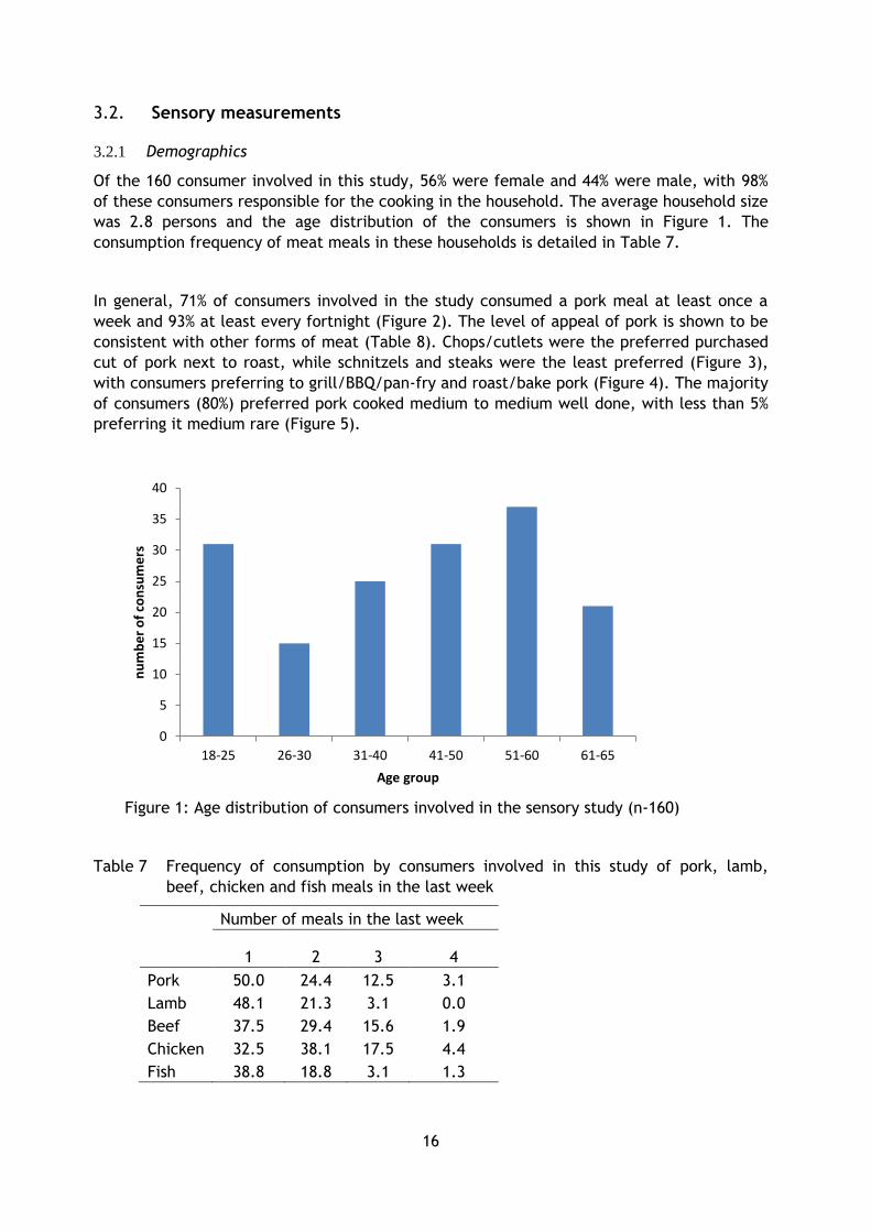
Of the 160 consumer involved in this study, 56% were female and 44% were male, with 98%
of these consumers responsible for the cooking in the household. The average household size
was 2.8 persons and the age distribution of the consumers is shown in Figure 1. The
consumption frequency of meat meals in these households is detailed in Table 7.
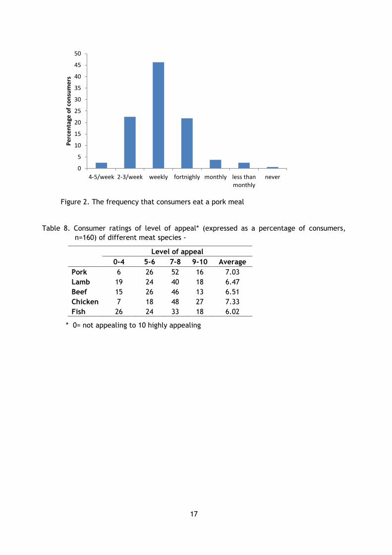
In general, 71% of consumers involved in the study consumed a pork meal at least once a
week and 93% at least every fortnight (Figure 2). The level of appeal of pork is shown to be
consistent with other forms of meat (Table 8). Chops/cutlets were the preferred purchased
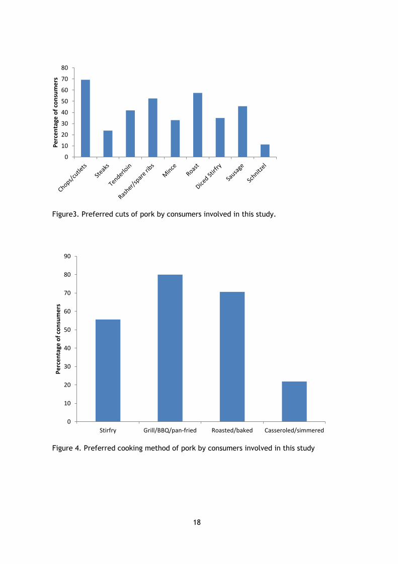
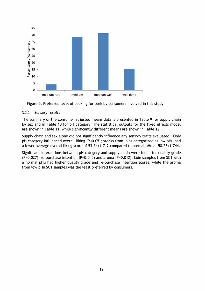
cut of pork next to roast, while schnitzels and steaks were the least preferred (Figure 3),
with consumers preferring to grill/BBQ/pan-fry and roast/bake pork (Figure 4). The majority
of consumers (80%) preferred pork cooked medium to medium well done, with less than 5%
preferring it medium rare (Figure 5).
Figure 1: Age distribution of consumers involved in the sensory study (n-160)
Table 7 Frequency of consumption by consumers involved in this study of pork, lamb,
beef, chicken and fish meals in the last week
Number of meals in the last week
1 2 3 4
Pork 50.0 24.4 12.5 3.1
Lamb 48.1 21.3 3.1 0.0
Beef 37.5 29.4 15.6 1.9
Chicken 32.5 38.1 17.5 4.4
Fish 38.8 18.8 3.1 1.3
0
5
10
15
20
25
30
35
40
18-25 26-30 31-40 41-50 51-60 61-65
nu
mb
er
of
con
sum
ers
Age group
17
Figure 2. The frequency that consumers eat a pork meal
Table 8. Consumer ratings of level of appeal* (expressed as a percentage of consumers,
n=160) of different meat species -
Level of appeal
0-4 5-6 7-8 9-10 Average
Pork 6 26 52 16 7.03
Lamb 19 24 40 18 6.47
Beef 15 26 46 13 6.51
Chicken 7 18 48 27 7.33
Fish 26 24 33 18 6.02
* 0= not appealing to 10 highly appealing
0
5
10
15
20
25
30
35
40
45
50
4-5/week 2-3/week weekly fortnighly monthly less thanmonthly
never
Pe
rce
nta
ge o
f co
nsu
me
rs
18
Figure3. Preferred cuts of pork by consumers involved in this study.
Figure 4. Preferred cooking method of pork by consumers involved in this study
0
10
20
30
40
50
60
70
80
Pe
rce
nta
ge o
f co
nsu
me
rs
0
10
20
30
40
50
60
70
80
90
Stirfry Grill/BBQ/pan-fried Roasted/baked Casseroled/simmered
Pe
rce
nta
ge o
f co
nsu
me
rs
19
Figure 5. Preferred level of cooking for pork by consumers involved in this study
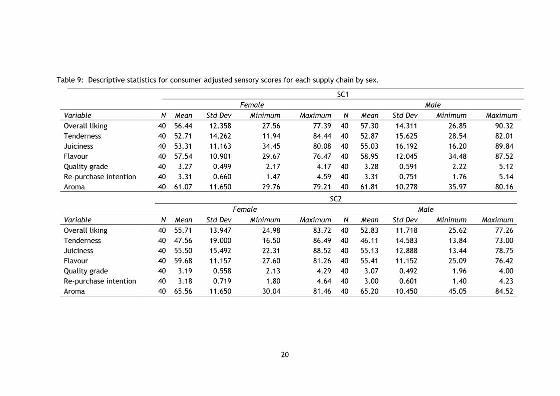
3.2.2 Sensory results
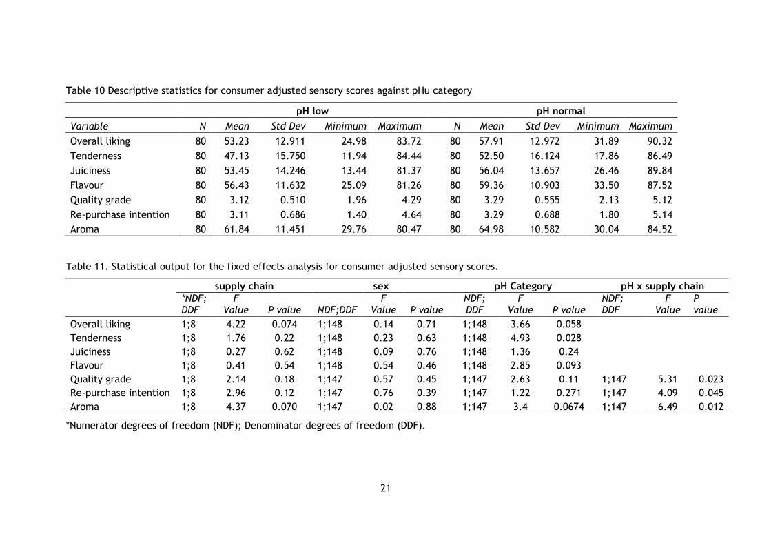
The summary of the consumer adjusted means data is presented in Table 9 for supply chain
by sex and in Table 10 for pH category. The statistical outputs for the fixed effects model
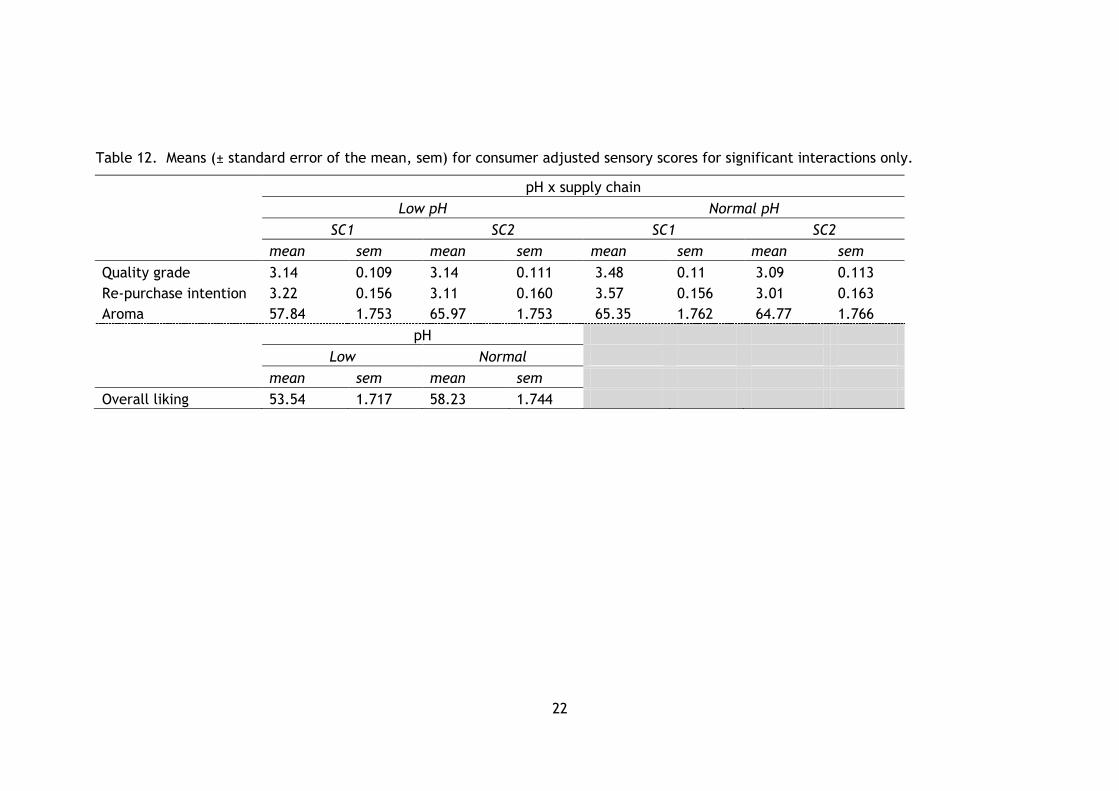
are shown in Table 11, while significantly different means are shown in Table 12.
Supply chain and sex alone did not significantly influence any sensory traits evaluated. Only
pH category influenced overall liking (P<0.05); steaks from loins categorized as low pHu had
a lower average overall liking score of 53.54±1.712 compared to normal pHu at 58.23±1.744.
Significant interactions between pH category and supply chain were found for quality grade
(P=0.027), re-purchase intention (P=0.045) and aroma (P=0.012). Loin samples from SC1 with
a normal pHu had higher quality grade and re-purchase intention scores, while the aroma
from low pHu SC1 samples was the least preferred by consumers.
0
5
10
15
20
25
30
35
40
45
medium rare medium medium well well done
Pe
rce
nta
ge o
f co
nsu
me
rs
20
Table 9: Descriptive statistics for consumer adjusted sensory scores for each supply chain by sex.
SC1
Female Male
Variable N Mean Std Dev Minimum Maximum N Mean Std Dev Minimum Maximum
Overall liking 40 56.44 12.358 27.56 77.39 40 57.30 14.311 26.85 90.32
Tenderness 40 52.71 14.262 11.94 84.44 40 52.87 15.625 28.54 82.01
Juiciness 40 53.31 11.163 34.45 80.08 40 55.03 16.192 16.20 89.84
Flavour 40 57.54 10.901 29.67 76.47 40 58.95 12.045 34.48 87.52
Quality grade 40 3.27 0.499 2.17 4.17 40 3.28 0.591 2.22 5.12
Re-purchase intention 40 3.31 0.660 1.47 4.59 40 3.31 0.751 1.76 5.14
Aroma 40 61.07 11.650 29.76 79.21 40 61.81 10.278 35.97 80.16
SC2
Female Male
Variable N Mean Std Dev Minimum Maximum N Mean Std Dev Minimum Maximum
Overall liking 40 55.71 13.947 24.98 83.72 40 52.83 11.718 25.62 77.26
Tenderness 40 47.56 19.000 16.50 86.49 40 46.11 14.583 13.84 73.00
Juiciness 40 55.50 15.492 22.31 88.52 40 55.13 12.888 13.44 78.75
Flavour 40 59.68 11.157 27.60 81.26 40 55.41 11.152 25.09 76.42
Quality grade 40 3.19 0.558 2.13 4.29 40 3.07 0.492 1.96 4.00
Re-purchase intention 40 3.18 0.719 1.80 4.64 40 3.00 0.601 1.40 4.23
Aroma 40 65.56 11.650 30.04 81.46 40 65.20 10.450 45.05 84.52
21
Table 10 Descriptive statistics for consumer adjusted sensory scores against pHu category
pH low pH normal
Variable N Mean Std Dev Minimum Maximum N Mean Std Dev Minimum Maximum
Overall liking 80 53.23 12.911 24.98 83.72 80 57.91 12.972 31.89 90.32
Tenderness 80 47.13 15.750 11.94 84.44 80 52.50 16.124 17.86 86.49
Juiciness 80 53.45 14.246 13.44 81.37 80 56.04 13.657 26.46 89.84
Flavour 80 56.43 11.632 25.09 81.26 80 59.36 10.903 33.50 87.52
Quality grade 80 3.12 0.510 1.96 4.29 80 3.29 0.555 2.13 5.12
Re-purchase intention 80 3.11 0.686 1.40 4.64 80 3.29 0.688 1.80 5.14
Aroma 80 61.84 11.451 29.76 80.47 80 64.98 10.582 30.04 84.52
Table 11. Statistical output for the fixed effects analysis for consumer adjusted sensory scores.
supply chain sex pH Category pH x supply chain
*NDF; DDF
F Value P value NDF;DDF
F Value P value
NDF; DDF
F Value P value
NDF; DDF
F Value
P value
Overall liking 1;8 4.22 0.074 1;148 0.14 0.71 1;148 3.66 0.058
Tenderness 1;8 1.76 0.22 1;148 0.23 0.63 1;148 4.93 0.028 Juiciness 1;8 0.27 0.62 1;148 0.09 0.76 1;148 1.36 0.24 Flavour 1;8 0.41 0.54 1;148 0.54 0.46 1;148 2.85 0.093 Quality grade 1;8 2.14 0.18 1;147 0.57 0.45 1;147 2.63 0.11 1;147 5.31 0.023
Re-purchase intention 1;8 2.96 0.12 1;147 0.76 0.39 1;147 1.22 0.271 1;147 4.09 0.045
Aroma 1;8 4.37 0.070 1;147 0.02 0.88 1;147 3.4 0.0674 1;147 6.49 0.012
*Numerator degrees of freedom (NDF); Denominator degrees of freedom (DDF).
22
Table 12. Means (± standard error of the mean, sem) for consumer adjusted sensory scores for significant interactions only.
pH x supply chain
Low pH Normal pH
SC1 SC2 SC1 SC2
mean sem mean sem mean sem mean sem
Quality grade 3.14 0.109 3.14 0.111 3.48 0.11 3.09 0.113
Re-purchase intention 3.22 0.156 3.11 0.160 3.57 0.156 3.01 0.163
Aroma 57.84 1.753 65.97 1.753 65.35 1.762 64.77 1.766
pH
Low Normal
mean sem mean sem
Overall liking 53.54 1.717 58.23 1.744
23
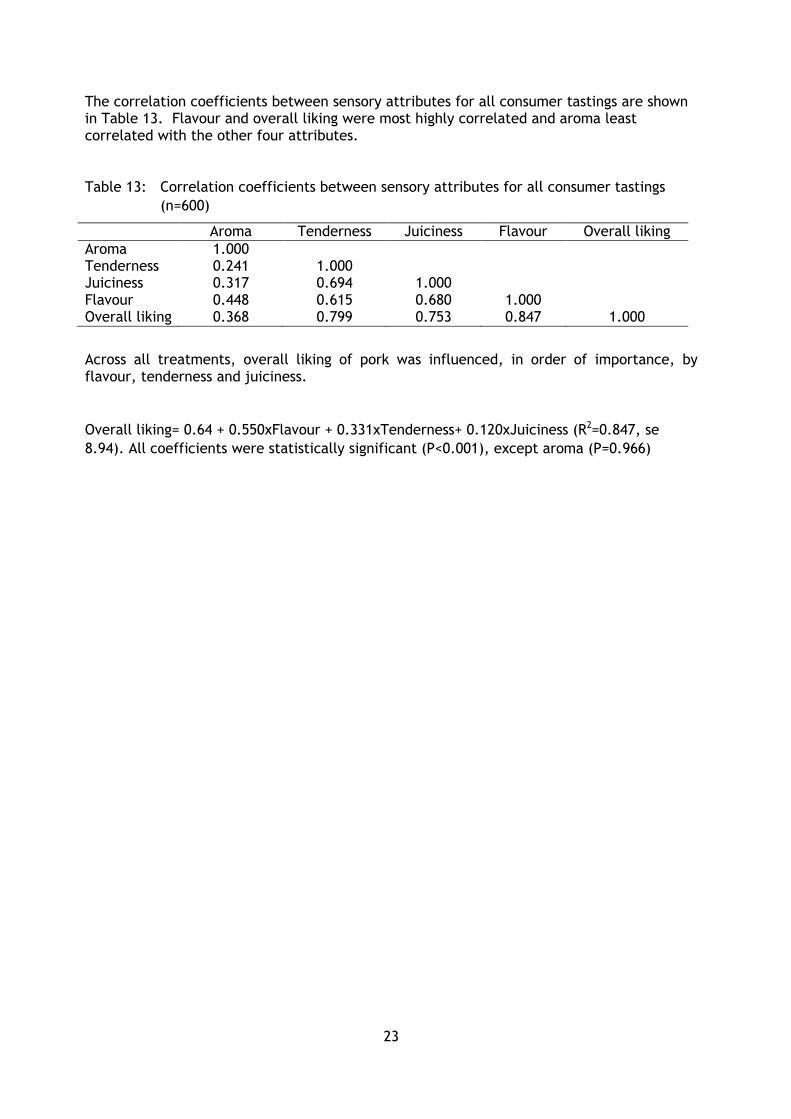
The correlation coefficients between sensory attributes for all consumer tastings are shown in Table 13. Flavour and overall liking were most highly correlated and aroma least correlated with the other four attributes.
Table 13: Correlation coefficients between sensory attributes for all consumer tastings
(n=600)
Aroma Tenderness Juiciness Flavour Overall liking
Aroma 1.000 Tenderness 0.241 1.000 Juiciness 0.317 0.694 1.000 Flavour 0.448 0.615 0.680 1.000 Overall liking 0.368 0.799 0.753 0.847 1.000
Across all treatments, overall liking of pork was influenced, in order of importance, by flavour, tenderness and juiciness.
Overall liking= 0.64 + 0.550xFlavour + 0.331xTenderness+ 0.120xJuiciness (R2=0.847, se
8.94). All coefficients were statistically significant (P<0.001), except aroma (P=0.966)
24
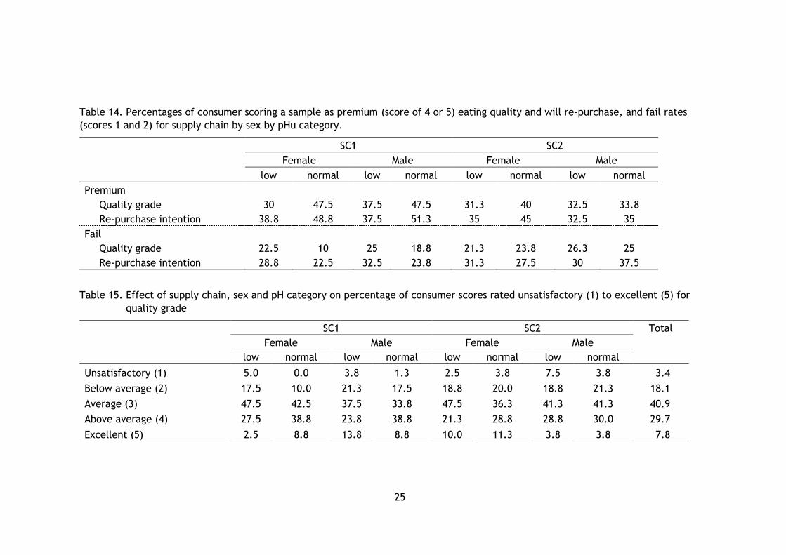
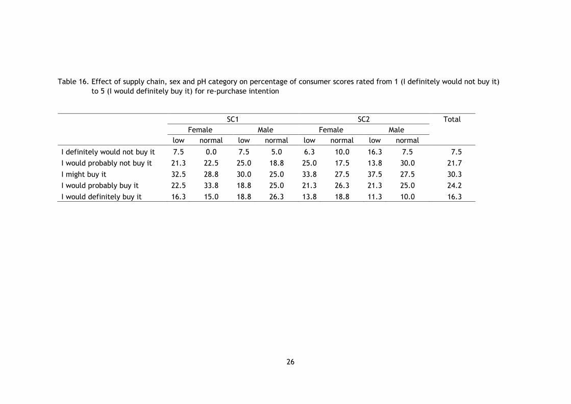
3.2.3 Sensory fail and premium rates
The percentage of samples that scored either 1 or 2 (fail) or 4 or 5 (premium) on both
quality grade and re-purchase intention are presented in Table 14. The overall score matrix
are presented in Tables 15 and 16. Steaks obtaining scores of 1 or 2 are considered to fail in
eating quality. Of all the steaks tasted, 21% were considered to have poor eating quality and
29% of consumers would not re-purchase a loin steak that they tasted. Loin steaks from
females in a normal pHu range performed the best with the lowest fail rates, while males
from SC2 consistently had the highest fail rate despite the pH category.
Overall, 29.7% of samples were graded as above average (4) and 7.8% as excellent (5). These
were also reflected in the re-purchasing decisions of consumers, with 24.2% of steaks
obtaining a rating of probably would buy (4) 24.2% and 16.3% of steaks were rated as
definitely would buy (5). Of all these, normal pH steaks from SC1 seemed to perform the
best, with a greater number of steaks performing at a premium level compared to the other
treatments.
25
Table 14. Percentages of consumer scoring a sample as premium (score of 4 or 5) eating quality and will re-purchase, and fail rates
(scores 1 and 2) for supply chain by sex by pHu category.
SC1 SC2
Female Male Female Male
low normal low normal low normal low normal
Premium
Quality grade 30 47.5 37.5 47.5 31.3 40 32.5 33.8
Re-purchase intention 38.8 48.8 37.5 51.3 35 45 32.5 35
Fail
Quality grade 22.5 10 25 18.8 21.3 23.8 26.3 25
Re-purchase intention 28.8 22.5 32.5 23.8 31.3 27.5 30 37.5
Table 15. Effect of supply chain, sex and pH category on percentage of consumer scores rated unsatisfactory (1) to excellent (5) for
quality grade
SC1 SC2 Total
Female Male Female Male
low normal low normal low normal low normal
Unsatisfactory (1) 5.0 0.0 3.8 1.3 2.5 3.8 7.5 3.8 3.4
Below average (2) 17.5 10.0 21.3 17.5 18.8 20.0 18.8 21.3 18.1
Average (3) 47.5 42.5 37.5 33.8 47.5 36.3 41.3 41.3 40.9
Above average (4) 27.5 38.8 23.8 38.8 21.3 28.8 28.8 30.0 29.7
Excellent (5) 2.5 8.8 13.8 8.8 10.0 11.3 3.8 3.8 7.8
26
Table 16. Effect of supply chain, sex and pH category on percentage of consumer scores rated from 1 (I definitely would not buy it)
to 5 (I would definitely buy it) for re-purchase intention
SC1 SC2 Total
Female Male Female Male
low normal low normal low normal low normal
I definitely would not buy it 7.5 0.0 7.5 5.0 6.3 10.0 16.3 7.5 7.5
I would probably not buy it 21.3 22.5 25.0 18.8 25.0 17.5 13.8 30.0 21.7
I might buy it 32.5 28.8 30.0 25.0 33.8 27.5 37.5 27.5 30.3
I would probably buy it 22.5 33.8 18.8 25.0 21.3 26.3 21.3 25.0 24.2
I would definitely buy it 16.3 15.0 18.8 26.3 13.8 18.8 11.3 10.0 16.3
27
3.3. pH analysis
Whilst an analysis of pHu category as a fixed effect and the treatment interactions involved
offer an insight into the relationships of pHu, objective measures and sensory scores, the
true relationship against a continuous range of pHu may provide a better understanding of
these effects. This section presents data from an analysis using pH as a continuous variable
against consumer sensory scores and meat quality objective measurements.
3.3.1 Effect of pHu on consumer sensory scores
The correlation coefficients for pHu and pH24 with the consumer sensory scores are shown
in Table 17. All sensory scores correlated significantly with pHu except juiciness and aroma.
Although these correlations were relatively weak, no correlations between pH24 and sensory
scores existed. There was a stronger correlation between pHu and pH24; however this
correlation was not as strong as expected since pH24 is often used as an indicator of
ultimate pH.
Table 17. Correlation coefficients for pHu and pH24 between
consumer adjusted sensory scores
pHu pH24
pHu 1.000 pH24 0.357*** 1.000
Overall liking 0.204** -0.079
Tenderness 0.190* -0.115
Juiciness 0.120 -0.024
Flavour 0.173* -0.069
Quality grade 0.196* -0.051
Re-purchase intention 0.165* -0.045
Aroma 0.147 0.016
*** P<0.001; **P<0.01; *P<0.05.
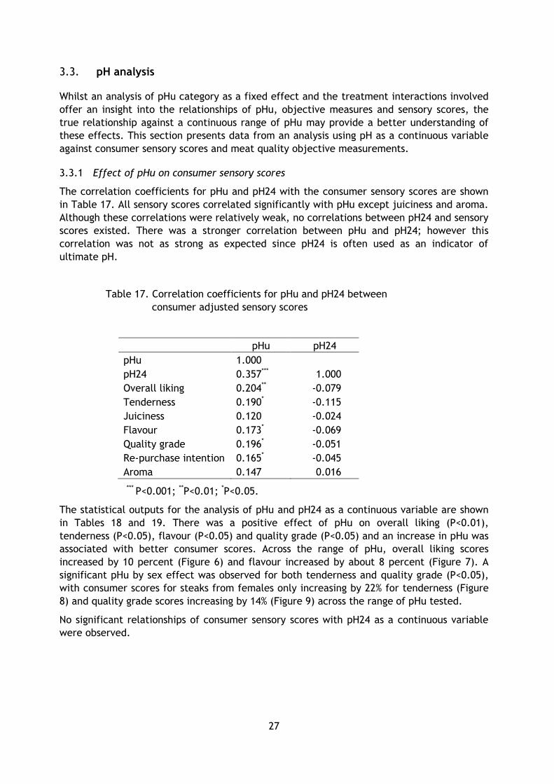
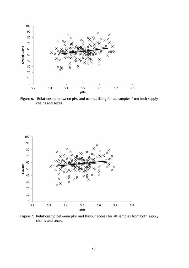
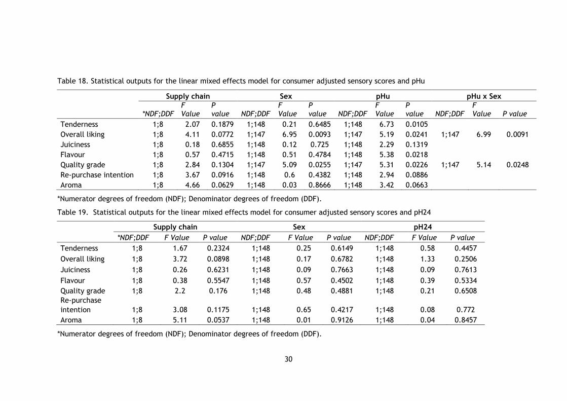
The statistical outputs for the analysis of pHu and pH24 as a continuous variable are shown
in Tables 18 and 19. There was a positive effect of pHu on overall liking (P<0.01),
tenderness (P<0.05), flavour (P<0.05) and quality grade (P<0.05) and an increase in pHu was
associated with better consumer scores. Across the range of pHu, overall liking scores
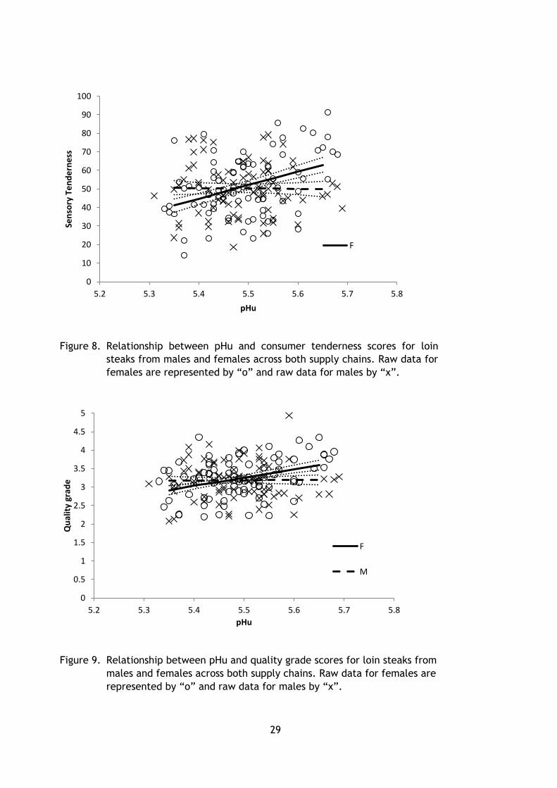
increased by 10 percent (Figure 6) and flavour increased by about 8 percent (Figure 7). A
significant pHu by sex effect was observed for both tenderness and quality grade (P<0.05),
with consumer scores for steaks from females only increasing by 22% for tenderness (Figure
8) and quality grade scores increasing by 14% (Figure 9) across the range of pHu tested.
No significant relationships of consumer sensory scores with pH24 as a continuous variable
were observed.
28
Figure 6. Relationship between pHu and overall liking for all samples from both supply
chains and sexes.
Figure 7. Relationship between pHu and flavour scores for all samples from both supply
chains and sexes.
0
10
20
30
40
50
60
70
80
90
100
5.2 5.3 5.4 5.5 5.6 5.7 5.8
Ove
rall
Liki
ng
pHu
0
10
20
30
40
50
60
70
80
90
100
5.2 5.3 5.4 5.5 5.6 5.7 5.8
Flav
ou
r
pHu
29
Figure 8. Relationship between pHu and consumer tenderness scores for loin
steaks from males and females across both supply chains. Raw data for
females are represented by “o” and raw data for males by “x”.
Figure 9. Relationship between pHu and quality grade scores for loin steaks from
males and females across both supply chains. Raw data for females are
represented by “o” and raw data for males by “x”.
0
10
20
30
40
50
60
70
80
90
100
5.2 5.3 5.4 5.5 5.6 5.7 5.8
Sen
sory
Te
nd
ern
ess
pHu
F
0
0.5
1
1.5
2
2.5
3
3.5
4
4.5
5
5.2 5.3 5.4 5.5 5.6 5.7 5.8
Qu
alit
y gr
ade
pHu
F
M
30
Table 18. Statistical outputs for the linear mixed effects model for consumer adjusted sensory scores and pHu
Supply chain Sex pHu pHu x Sex
*NDF;DDF F Value
P value NDF;DDF
F Value
P value NDF;DDF
F Value
P value NDF;DDF
F Value P value
Tenderness 1;8 2.07 0.1879 1;148 0.21 0.6485 1;148 6.73 0.0105 Overall liking 1;8 4.11 0.0772 1;147 6.95 0.0093 1;147 5.19 0.0241 1;147 6.99 0.0091
Juiciness 1;8 0.18 0.6855 1;148 0.12 0.725 1;148 2.29 0.1319 Flavour 1;8 0.57 0.4715 1;148 0.51 0.4784 1;148 5.38 0.0218 Quality grade 1;8 2.84 0.1304 1;147 5.09 0.0255 1;147 5.31 0.0226 1;147 5.14 0.0248
Re-purchase intention 1;8 3.67 0.0916 1;148 0.6 0.4382 1;148 2.94 0.0886 Aroma 1;8 4.66 0.0629 1;148 0.03 0.8666 1;148 3.42 0.0663
*Numerator degrees of freedom (NDF); Denominator degrees of freedom (DDF).
Table 19. Statistical outputs for the linear mixed effects model for consumer adjusted sensory scores and pH24
Supply chain Sex pH24
*NDF;DDF F Value P value NDF;DDF F Value P value NDF;DDF F Value P value
Tenderness 1;8 1.67 0.2324 1;148 0.25 0.6149 1;148 0.58 0.4457
Overall liking 1;8 3.72 0.0898 1;148 0.17 0.6782 1;148 1.33 0.2506
Juiciness 1;8 0.26 0.6231 1;148 0.09 0.7663 1;148 0.09 0.7613
Flavour 1;8 0.38 0.5547 1;148 0.57 0.4502 1;148 0.39 0.5334
Quality grade 1;8 2.2 0.176 1;148 0.48 0.4881 1;148 0.21 0.6508
Re-purchase
intention 1;8 3.08 0.1175 1;148 0.65 0.4217 1;148 0.08 0.772
Aroma 1;8 5.11 0.0537 1;148 0.01 0.9126 1;148 0.04 0.8457
*Numerator degrees of freedom (NDF); Denominator degrees of freedom (DDF).
31
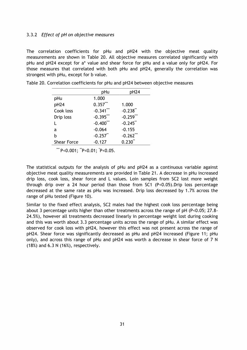
3.3.2 Effect of pH on objective measures
The correlation coefficients for pHu and pH24 with the objective meat quality
measurements are shown in Table 20. All objective measures correlated significantly with
pHu and pH24 except for a* value and shear force for pHu and a value only for pH24. For
those measures that correlated with both pHu and pH24, generally the correlation was
strongest with pHu, except for b value.
Table 20. Correlation coefficients for pHu and pH24 between objective measures
pHu pH24
pHu 1.000
pH24 0.357*** 1.000
Cook loss -0.341*** -0.238**
Drip loss -0.395*** -0.259***
L -0.400*** -0.245**
a -0.064 -0.155
b -0.257** -0.262***
Shear Force -0.127 0.230**
*** P<0.001; **P<0.01; *P<0.05.
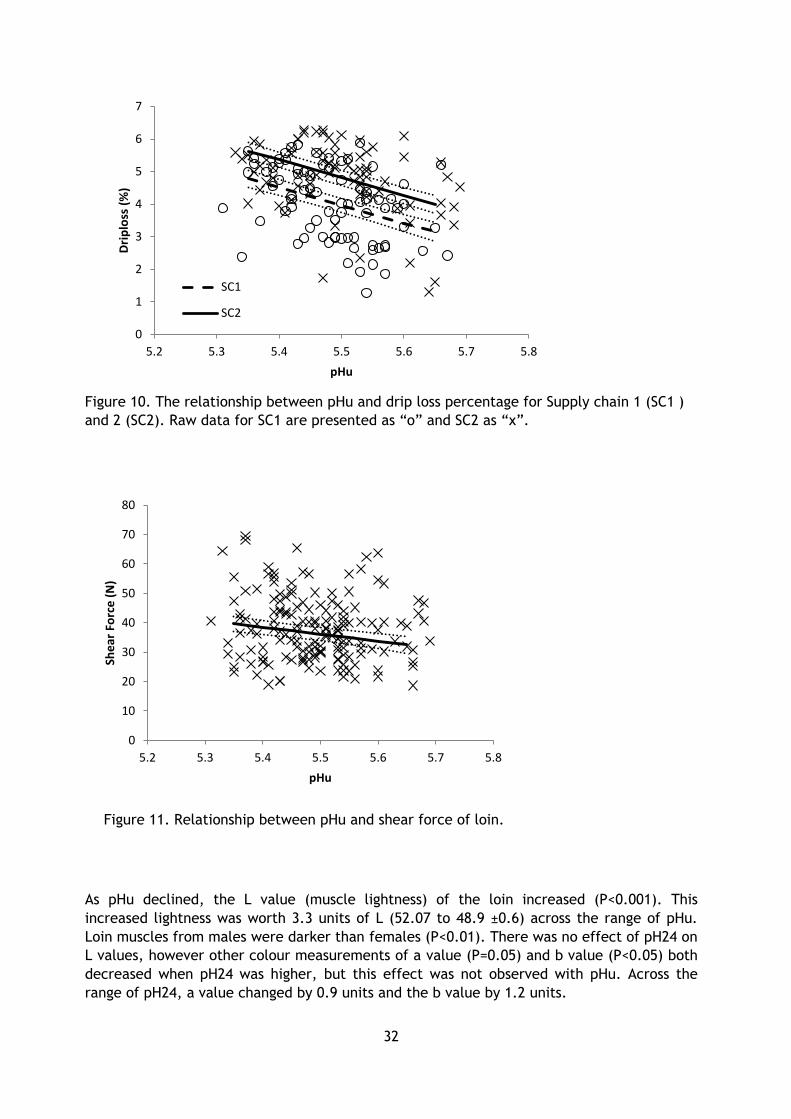
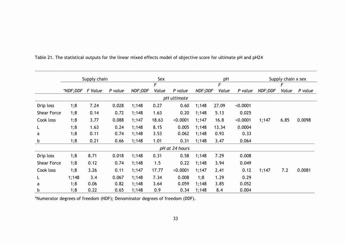
The statistical outputs for the analysis of pHu and pH24 as a continuous variable against
objective meat quality measurements are provided in Table 21. A decrease in pHu increased
drip loss, cook loss, shear force and L values. Loin samples from SC2 lost more weight
through drip over a 24 hour period than those from SC1 (P<0.05).Drip loss percentage
decreased at the same rate as pHu was increased. Drip loss decreased by 1.7% across the
range of pHu tested (Figure 10).
Similar to the fixed effect analysis, SC2 males had the highest cook loss percentage being
about 3 percentage units higher than other treatments across the range of pH (P<0.05; 27.8-
24.5%), however all treatments decreased linearly in percentage weight lost during cooking
and this was worth about 3.3 percentage units across the range of pHu. A similar effect was
observed for cook loss with pH24, however this effect was not present across the range of
pH24. Shear force was significantly decreased as pHu and pH24 increased (Figure 11; pHu
only), and across this range of pHu and pH24 was worth a decrease in shear force of 7 N
(18%) and 6.3 N (16%), respectively.
32
Figure 10. The relationship between pHu and drip loss percentage for Supply chain 1 (SC1 )
and 2 (SC2). Raw data for SC1 are presented as “o” and SC2 as “x”.
Figure 11. Relationship between pHu and shear force of loin.
As pHu declined, the L value (muscle lightness) of the loin increased (P<0.001). This
increased lightness was worth 3.3 units of L (52.07 to 48.9 ±0.6) across the range of pHu.
Loin muscles from males were darker than females (P<0.01). There was no effect of pH24 on
L values, however other colour measurements of a value (P=0.05) and b value (P<0.05) both
decreased when pH24 was higher, but this effect was not observed with pHu. Across the
range of pH24, a value changed by 0.9 units and the b value by 1.2 units.
0
1
2
3
4
5
6
7
5.2 5.3 5.4 5.5 5.6 5.7 5.8
Dri
plo
ss (
%)
pHu
SC1
SC2
0
10
20
30
40
50
60
70
80
5.2 5.3 5.4 5.5 5.6 5.7 5.8
She
ar F
orc
e (
N)
pHu
33
Table 21. The statistical outputs for the linear mixed effects model of objective score for ultimate pH and pH24
Supply chain Sex pH Supply chain x sex
*NDF;DDF F Value P value NDF;DDF
F
Value P value NDF;DDF
F
Value P value NDF;DDF
F
Value P value
pH ultimate
Drip loss 1;8 7.24 0.028 1;148 0.27 0.60 1;148 27.09 <0.0001
Shear Force 1;8 0.14 0.72 1;148 1.63 0.20 1;148 5.13 0.025
Cook loss 1;8 3.77 0.088 1;147 18.63 <0.0001 1;147 16.8 <0.0001 1;147 6.85 0.0098
L 1;8 1.63 0.24 1;148 8.15 0.005 1;148 13.34 0.0004
a 1;8 0.11 0.74 1;148 3.53 0.062 1;148 0.93 0.33
b 1;8 0.21 0.66 1;148 1.01 0.31 1;148 3.47 0.064
pH at 24 hours
Drip loss 1;8 8.71 0.018 1;148 0.31 0.58 1;148 7.29 0.008
Shear Force 1;8 0.12 0.74 1;148 1.5 0.22 1;148 3.94 0.049
Cook loss 1;8 3.26 0.11 1;147 17.77 <0.0001 1;147 2.41 0.12 1;147 7.2 0.0081
L 1;148 3.4 0.067 1;148 7.34 0.008 1;8 1.29 0.29
a 1;8 0.06 0.82 1;148 3.64 0.059 1;148 3.85 0.052
b 1;8 0.22 0.65 1;148 0.9 0.34 1;148 8.4 0.004
*Numerator degrees of freedom (NDF); Denominator degrees of freedom (DDF).
34
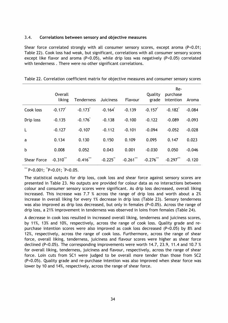
3.4. Correlations between sensory and objective measures
Shear force correlated strongly with all consumer sensory scores, except aroma (P<0.01;
Table 22). Cook loss had weak, but significant, correlations with all consumer sensory scores
except like flavor and aroma (P<0.05), while drip loss was negatively (P<0.05) correlated
with tenderness . There were no other significant correlations.
Table 22. Correlation coefficient matrix for objective measures and consumer sensory scores
Overall
liking Tenderness Juiciness Flavour
Quality
grade
Re-
purchase
intention Aroma
Cook loss -0.177* -0.173* -0.164* -0.139 -0.157* -0.182* -0.084
Drip loss -0.135 -0.176* -0.138 -0.100 -0.122 -0.089 -0.093
L -0.127 -0.107 -0.112 -0.101 -0.094 -0.052 -0.028
a 0.134 0.130 0.150 0.109 0.095 0.147 0.023
b 0.008 0.052 0.043 0.001 -0.030 0.050 -0.046
Shear Force -0.310*** -0.416*** -0.225** -0.261*** -0.276*** -0.297*** -0.120
*** P<0.001; **P<0.01; *P<0.05.
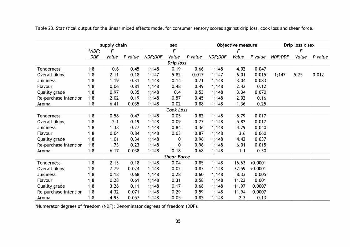
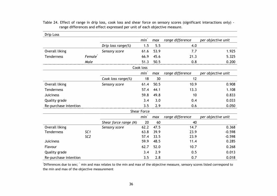
The statistical outputs for drip loss, cook loss and shear force against sensory scores are
presented in Table 23. No outputs are provided for colour data as no interactions between
colour and consumer sensory scores were significant. As drip loss decreased, overall liking
increased. This increase was 7.7 % across the range of drip loss and worth about a 2%
increase in overall liking for every 1% decrease in drip loss (Table 23). Sensory tenderness
was also improved as drip loss decreased, but only in females (P<0.05). Across the range of
drip loss, a 21% improvement in tenderness was observed in loins from females (Table 24).
A decrease in cook loss resulted in increased overall liking, tenderness and juiciness scores,
by 11%, 13% and 10%, respectively, across the range of cook loss. Quality grade and re-
purchase intention scores were also improved as cook loss decreased (P<0.05) by 8% and
12%, respectively, across the range of cook loss. Furthermore, across the range of shear
force, overall liking, tenderness, juiciness and flavour scores were higher as shear force
declined (P<0.05). The corresponding improvements were worth 14.7, 23.9, 11.4 and 10.7 %
for overall liking, tenderness, juiciness and flavour, respectively, across the range of shear
force. Loin cuts from SC1 were judged to be overall more tender than those from SC2
(P<0.05). Quality grade and re-purchase intention was also improved when shear force was
lower by 10 and 14%, respectively, across the range of shear force.
35
Table 23. Statistical output for the linear mixed effects model for consumer sensory scores against drip loss, cook loss and shear force.
supply chain sex Objective measure Drip loss x sex
*NDF;
DDF
F
Value P value NDF;DDF
F
Value P value NDF;DDF
F
Value P value NDF;DDF
F
Value P value
Drip loss
Tenderness 1;8 0.6 0.45 1;148 0.19 0.66 1;148 4.02 0.047
Overall liking 1;8 2.11 0.18 1;147 5.82 0.017 1;147 6.01 0.015 1;147 5.75 0.012
Juiciness 1;8 1.19 0.31 1;148 0.14 0.71 1;148 3.04 0.083
Flavour 1;8 0.06 0.81 1;148 0.48 0.49 1;148 2.42 0.12
Quality grade 1;8 0.97 0.35 1;148 0.4 0.53 1;148 3.34 0.070
Re-purchase intention 1;8 2.02 0.19 1;148 0.57 0.45 1;148 2.02 0.16
Aroma 1;8 6.41 0.035 1;148 0.02 0.88 1;148 1.36 0.25
Cook Loss
Tenderness 1;8 0.58 0.47 1;148 0.05 0.82 1;148 5.79 0.017
Overall liking 1;8 2.1 0.19 1;148 0.09 0.77 1;148 5.82 0.017
Juiciness 1;8 1.38 0.27 1;148 0.84 0.36 1;148 4.29 0.040
Flavour 1;8 0.04 0.84 1;148 0.03 0.87 1;148 3.6 0.060
Quality grade 1;8 1.01 0.34 1;148 0 0.96 1;148 4.42 0.037
Re-purchase intention 1;8 1.73 0.23 1;148 0 0.96 1;148 6.01 0.015
Aroma 1;8 6.17 0.038 1;148 0.18 0.68 1;148 1.1 0.30
Shear Force
Tenderness 1;8 2.13 0.18 1;148 0.04 0.85 1;148 16.63 <0.0001
Overall liking 1;8 7.79 0.024 1;148 0.02 0.87 1;148 32.59 <0.0001
Juiciness 1;8 0.18 0.68 1;148 0.28 0.60 1;148 8.33 0.005
Flavour 1;8 0.28 0.61 1;148 0.31 0.58 1;148 11.22 0.001
Quality grade 1;8 3.28 0.11 1;148 0.17 0.68 1;148 11.97 0.0007
Re-purchase intention 1;8 4.32 0.071 1;148 0.29 0.59 1;148 11.94 0.0007
Aroma 1;8 4.93 0.057 1;148 0.05 0.82 1;148 2.3 0.13
*Numerator degrees of freedom (NDF); Denominator degrees of freedom (DDF).
36
Table 24. Effect of range in drip loss, cook loss and shear force on sensory scores (significant interactions only) -
range differences and effect expressed per unit of each objective measure.
Drip Loss
min^ max range difference per objective unit
Drip loss range(%) 1.5 5.5 4.0
Overall liking Sensory score 61.6 53.9 7.7 1.925
Tenderness Female*
66.9 45.6 21.3 5.325
Male 51.3 50.5 0.8 0.200
Cook loss
min^ max range difference per objective unit
Cook loss range(%) 18 30 12
Overall liking Sensory score 61.4 50.5 10.9 0.908
Tenderness
57.4 44.1 13.3 1.108
Juiciness
59.8 49.8 10 0.833
Quality grade
3.4 3.0 0.4 0.033
Re-purchase intention 3.5 2.9 0.6 0.050
Shear Force
min^ max range difference per objective unit
Shear force range (N) 20 60 40
Overall liking Sensory score 62.2 47.5 14.7 0.368
Tenderness SC1
63.8 39.9 23.9 -0.598
SC2
57.4 33.5 23.9 -0.598
Juiciness
59.9 48.5 11.4 0.285
Flavour
62.7 52.0 10.7 0.268
Quality grade
3.4 2.9 0.5 0.013
Re-purchase intention 3.5 2.8 0.7 0.018
*Differences due to sex; ^ min and max relates to the min and max of the objective measure, sensory scores listed correspond to
the min and max of the objective measurement
37
3.5. Glycogen utilization
Correlations of pHu and pH24 for lactate (measured at 72 h post-slaughter), residual glucose
and total glycogen measured at slaughter are shown in Table 25. No pH category correlated
with the amount of lactate measured at 72 hours. There was a strong negative correlation
with pHu and residual glucose and total glycogen at slaughter (P<0.001), with a weaker
correlation for both residual glucose and total glycogen with pH24 (P<0.01).
Table 25. Correlation coefficients for pHu and pH24
against IMF and glycolytic potential
measures.
pHu pH24
IMF 0.047 0.062
Lactate -0.126 -0.105
Residual Glucose -0.554*** -0.235**
Glycogen -0.490*** -0.245**
*** P<0.001; **P<0.01; *P<0.05.
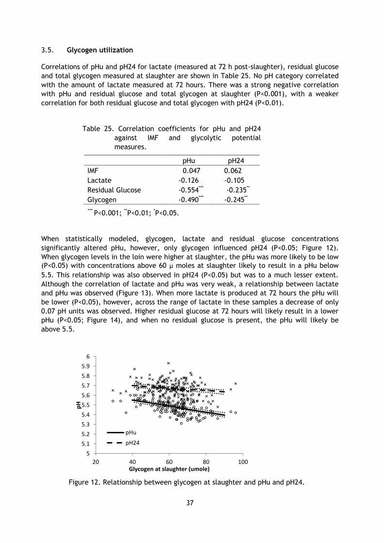
When statistically modeled, glycogen, lactate and residual glucose concentrations
significantly altered pHu, however, only glycogen influenced pH24 (P<0.05; Figure 12).
When glycogen levels in the loin were higher at slaughter, the pHu was more likely to be low
(P<0.05) with concentrations above 60 µ moles at slaughter likely to result in a pHu below
5.5. This relationship was also observed in pH24 (P<0.05) but was to a much lesser extent.
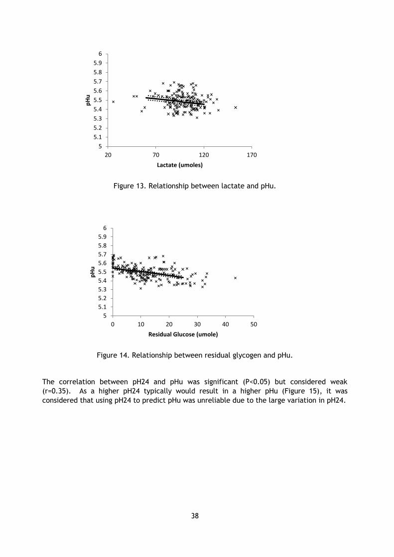
Although the correlation of lactate and pHu was very weak, a relationship between lactate
and pHu was observed (Figure 13). When more lactate is produced at 72 hours the pHu will
be lower (P<0.05), however, across the range of lactate in these samples a decrease of only
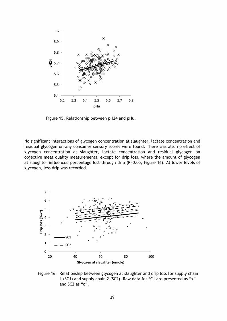
0.07 pH units was observed. Higher residual glucose at 72 hours will likely result in a lower
pHu (P<0.05; Figure 14), and when no residual glucose is present, the pHu will likely be
above 5.5.
Figure 12. Relationship between glycogen at slaughter and pHu and pH24.
5
5.1
5.2
5.3
5.4
5.5
5.6
5.7
5.8
5.9
6
20 40 60 80 100
pH
Glycogen at slaughter (umole)
pHu
pH24
38
Figure 13. Relationship between lactate and pHu.
Figure 14. Relationship between residual glycogen and pHu.
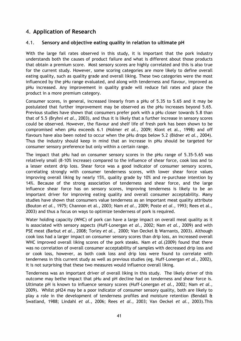
The correlation between pH24 and pHu was significant (P<0.05) but considered weak
(r=0.35). As a higher pH24 typically would result in a higher pHu (Figure 15), it was
considered that using pH24 to predict pHu was unreliable due to the large variation in pH24.
5
5.1
5.2
5.3
5.4
5.5
5.6
5.7
5.8
5.9
6
20 70 120 170
pH
u
Lactate (umoles)
5
5.1
5.2
5.3
5.4
5.5
5.6
5.7
5.8
5.9
6
0 10 20 30 40 50
pH
u
Residual Glucose (umole)
39
Figure 15. Relationship between pH24 and pHu.
No significant interactions of glycogen concentration at slaughter, lactate concentration and
residual glycogen on any consumer sensory scores were found. There was also no effect of
glycogen concentration at slaughter, lactate concentration and residual glycogen on
objective meat quality measurements, except for drip loss, where the amount of glycogen
at slaughter influenced percentage lost through drip (P<0.05; Figure 16). At lower levels of
glycogen, less drip was recorded.
Figure 16. Relationship between glycogen at slaughter and drip loss for supply chain
1 (SC1) and supply chain 2 (SC2). Raw data for SC1 are presented as “x”
and SC2 as “o”.
5.4
5.5
5.6
5.7
5.8
5.9
6
5.2 5.3 5.4 5.5 5.6 5.7 5.8
pH
24
pHu
0
1
2
3
4
5
6
7
20 40 60 80 100
Dri
p lo
ss (
%w
t)
Glycogen at slaughter (umole)
SC1
SC2

40
3.6. Intramuscular fat content
There were no significant interactions with treatment and or any measures or sensory scores
with IMF content, except b value (P<0.05). As IMF increased, steaks would be more yellow in
colour (data not shown). Additionally, there was a sex effect of IMF with P2 fat depth
(P<0.05). An increased P2 fat depth score increased the level of IMF in females, however,
increased P2 fat depth of male carcases led to a decrease in IMF in the loin.
41
4. Application of Research
4.1. Sensory and objective eating quality in relation to ultimate pH
With the large fail rates observed in this study, it is important that the pork industry
understands both the causes of product failure and what is different about those products
that obtain a premium score. Most sensory scores are highly correlated and this is also true
for the current study. However, some scoring categories are more likely to define overall
eating quality, such as quality grade and overall liking. These two categories were the most
influenced by the pHu range evaluated, and along with tenderness and flavour, improved as
pHu increased. Any improvement in quality grade will reduce fail rates and place the
product in a more premium category.
Consumer scores, in general, increased linearly from a pHu of 5.35 to 5.65 and it may be
postulated that further improvement may be observed as the pHu increases beyond 5.65.
Previous studies have shown that consumers prefer pork with a pHu closer towards 5.8 than
that of 5.5 (Bryhni et al., 2003), and thus it is likely that a further increase in sensory scores
could be observed. However, the flavour and shelf life of fresh pork has been shown to be
compromised when pHu exceeds 6.1 (Holmer et al., 2009; Klont et al., 1998) and off
flavours have also been noted to occur when the pHu drops below 5.2 (Bidner et al., 2004).
Thus the industry should keep in mind that an increase in pHu should be targeted for
consumer sensory preference but only within a certain range.
The impact that pHu had on consumer sensory scores in the pHu range of 5.35-5.65 was
relatively small (8-10% increase) compared to the influence of shear force, cook loss and to
a lesser extent drip loss. Shear force was a good indicator of consumer sensory scores,
correlating strongly with consumer tenderness scores, with lower shear force values
improving overall liking by nearly 15%, quality grade by 10% and re-purchase intention by
14%. Because of the strong association of tenderness and shear force, and the large
influence shear force has on sensory scores, improving tenderness is likely to be an
important driver for improving eating quality and overall consumer acceptability. Many
studies have shown that consumers value tenderness as an important meat quality attribute
(Bouton et al., 1975; Channon et al., 2003; Nam et al., 2009; Poste et al., 1993; Rees et al.,
2003) and thus a focus on ways to optimize tenderness of pork is required.
Water holding capacity (WHC) of pork can have a large impact on overall meat quality as it
is associated with sensory aspects (Huff-Lonergan et al., 2002; Nam et al., 2009) and with
PSE meat (Barbut et al., 2008; Torley et al., 2000; Van Oeckel & Warnants, 2003). Although
cook loss had a larger impact on consumer sensory scores than drip loss, an increased overall
WHC improved overall liking scores of the pork steaks. Nam et al.(2009) found that there
was no correlation of overall consumer acceptability of samples with decreased drip loss and
or cook loss, however, as both cook loss and drip loss were found to correlate with
tenderness in this current study as well as previous studies (eg. Huff-Lonergan et al., 2002),
it is not surprising that these two measures would influence overall liking.
Tenderness was an important driver of overall liking in this study. The likely driver of this
outcome may bethe impact that pHu and pH decline had on tenderness and shear force is.
Ultimate pH is known to influence sensory scores (Huff-Lonergan et al., 2002; Nam et al.,
2009). Whilst pH24 may be a poor indicator of consumer sensory quality, both are likely to
play a role in the development of tenderness profiles and moisture retention (Bendall &
Swatland, 1988; Lindahl et al., 2006; Rees et al., 2003; Van Oeckel et al., 2003).This
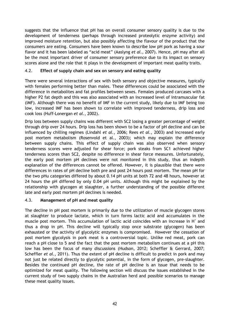
42
suggests that the influence that pH has on overall consumer sensory quality is due to the
development of tenderness (perhaps through increased proteolytic enzyme activity) and
improved moisture retention, but also possibly affecting the flavour of the product that the
consumers are eating. Consumers have been known to describe low pH pork as having a sour
flavor and it has been labeled as “acid meat” (Aaslyng et al., 2007). Hence, pH may after all
be the most important driver of consumer sensory preference due to its impact on sensory
scores alone and the role that it plays in the development of important meat quality traits.
4.2. Effect of supply chain and sex on sensory and eating quality
There were several interactions of sex with both sensory and objective measures, typically
with females performing better than males. These differences could be associated with the
difference in metabolites and fat profiles between sexes. Females produced carcases with a
higher P2 fat depth and this was also associated with an increased level of intramuscular fat
(IMF). Although there was no benefit of IMF in the current study, likely due to IMF being too
low, increased IMF has been shown to correlate with improved tenderness, drip loss and
cook loss (Huff-Lonergan et al., 2002).
Drip loss between supply chains was different with SC2 losing a greater percentage of weight
through drip over 24 hours. Drip loss has been shown to be a factor of pH decline and can be
influenced by chilling regimes (Lindahl et al., 2006; Rees et al., 2003) and increased early
post mortem metabolism (Rosenvold et al., 2003); which may explain the difference
between supply chains. This effect of supply chain was also observed when sensory
tenderness scores were adjusted for shear force; pork steaks from SC1 achieved higher
tenderness scores than SC2, despite no difference in shear force measures. Unfortunately,
the early post mortem pH declines were not monitored in this study, thus an indepth
explanation of the differences cannot be offered. However, it is plausible that there were
differences in rates of pH decline both pre and post 24 hours post mortem. The mean pH for
the two pHu categories differed by about 0.14 pH units at both 72 and 48 hours, however at
24 hours the pH differed by only 0.04 pH units. Although this might be explained by the
relationship with glycogen at slaughter, a further understanding of the possible different
late and early post mortem pH declines is needed.
4.3. Management of pH and meat quality
The decline in pH post mortem is primarily due to the utilization of muscle glycogen stores
at slaughter to produce lactate, which in turn forms lactic acid and accumulates in the
muscle post mortem. This accumulation of lactic acid coincides with an increase in H+ and
thus a drop in pH. This decline will typically stop once substrate (glycogen) has been
exhausted or the activity of glycolytic enzymes is compromised. However the cessation of
post mortem glycolysis in pork meat is a controversial topic. Unlike red meat, pork can
reach a pH close to 5 and the fact that the post mortem metabolism continues at a pH this
low has been the focus of many discussions (Hudson, 2012; Scheffler & Gerrard, 2007;
Scheffler et al., 2011). Thus the extent of pH decline is difficult to predict in pork and may
not just be related directly to glycolytic potential, in the form of glycogen, pre-slaughter.
Besides the continued pH decline, the rate of pH decline is an issue that needs to be
optimized for meat quality. The following section will discuss the issues established in the
current study of two supply chains in the Australian herd and possible scenarios to manage
these meat quality issues.
43
Within the past two decades, breeding programs in the pork industry have focused on
eliminating the Halothane and RN- genes which have been responsible for poor meat quality
(Barbut et al., 2008; Rosenvold & Andersen, 2003). Currently, breeding programs are based
around growth and increasing yield which may have an impact on meat quality traits. It has
been shown that pork with more type I and IIA muscle fibers will likely have decreased drip
loss, improved shear force and a higher early post mortem pH (Ryu & Kim, 2005), while pork
with a high content of type IIB fiber had low tenderness (Karlsson et al., 1993). However,
differences in fibre types do not necessarily influence sensory scores (Nam et al., 2009). The
differences observed in meat quality between type I/IIA and type IIB is likely due to the size
of fibers (Ryu et al., 2005) and the potential to store glycogen (Karlsson et al., 1999). Type
IIB fibers have fast twitch, glycolytic metabolic characteristics and a high glycogen content,
while type I has slow twitch, oxidative metabolic characteristics with low glycogen content
(Karlsson et al., 1999). Type IIA is an intermediate fast oxidative-glycolytic fiber. The
difference in meat quality attributes between these fibre types is a direct result of the
differing ability to store muscle glycogen.
In the current data set, larger pools of muscle glycogen at slaughter resulted in a lower pHu
and pH24. These findings are supported by Choe et al.(2008). They found that higher
glycogen stores are associated with faster early pH decline and lower pH24. Their findings
were also associated with increased percentage of type IIB fibers. The current status of fibre
type composition in the Australian herd is unknown, however the loin muscle is more
glycolytic than oxidative and theoretically could have lower meat quality than muscles with
a more oxidative potential. An investigation into optimizing the composition of fiber types
for meat quality while maintaining good yield is essential. This work must also extend
beyond the loin muscle.
High glycogen levels are likely to impact on pH decline and meat quality and many studies
have investigated nutritional means to lower glycogen at slaughter to improve meat quality.
Strategic finishing diets have been shown to reduce muscle glycogen and improve meat
quality, namely WHC (Rosenvold et al., 2001; Rosenvold et al., 2002). Diets containing high
fat (17-18%) and protein (22-24%) with low contents of digestible carbohydrate (<5%) were
required to reduce muscle glycogen stores in the loin muscle without affecting performance
(Rosenvold et al., 2001; Rosenvold et al., 2002). The high ratio of fat to carbohydrate is
essential in replicating this effect on muscle glycogen stores (Rosenvold et al., 2003). It was
also found that this improvement in meat quality was due to a higher pH at 45 minutes post
slaughter and not an increase in pH24 (Rosenvold et al., 2001; Rosenvold et al., 2002; Tikk,
et al., 2006). Although the true ultimate pH was not measured, it seems likely, due to the
current data and the relationship of glycogen and pH, that pHu could be increased with
strategic feeding. It has been shown that magnesium supplementation prior to slaughter
improves pork quality by improving WHC (D'Souza et al., 1999; D'Souza et al., 2000) and
these differences are likely due to increased lactate production immediately post slaughter
(D'Souza et al., 1999). The increased early metabolism could be explained by the discovery
of two different pools of glycogen. Firstly, a smaller pool, named proglycogen is degraded in
favour of the larger pool, macroglycogen (Rosenvold et al., 2003), and the rate that
proglycogen is metabolized will drive early post mortem glycolysis. Additionally, when
glycogen-reducing feeding strategies are implemented, a reduction in macroglycogen pools
and not proglycogen are observed, however, this interaction leads to a decreased rate of
proglycogen metabolism (Rosenvold et al., 2003). Thus, differences in drip loss between
supply chains could be a result of early post mortem metabolism and this may need to be
investigated in order to optimize early pH declines and WHC.
44
Processing techniques have been extensively studied in order to improve pork meat quality.
These technologies include, but are not limited to, chilling rates and electrical stimulation.
Each technology offers a significant benefit by altering pH declines and or the development
of tenderness. However, the timing post mortem and the pH-temperature dependence is
likely to be a large determinant of the meat quality outcomes (Rosenvold et al., 2003).
Channon et al.(2003) found that an accelerated pH decline as a consequence of electrical
stimulation at 2 minutes post slaughter resulted in lower shear force and higher sensory
tenderness scores, but did not affect on drip loss. The lack of effect of drip loss maybe due
to the timing of stimulation early post mortem, influencing the early pH decline which has
been shown to influence WHC (Rosenvold et al., 2003). Coincidently, Rees et al.,(2003)
found that early post mortem electrical stimulation increased drip loss. This resulted in a
faster pH decline and shear force was decreased and tenderness scores improved. Thus
implementing electrical stimulation is likely to improve tenderness development through an
increased pH decline, resulting in a lower pH at higher temperatures.
Conversely, rapid chilling has been shown to improve WHC (Juárez et al., 2009; Kerth et al.,
2001) but typically can result in tougher meat to conventionally chilled meat (van der Wal
et al., 1995), possibly due to slower pH declines (Tomović et al., 2008). Thus, it is of
significant importance for meat quality to optimize the pH-temperature window in which
chilling should commence for the development of tenderness and improved WHC.
Furthermore, this should also be adjusted for the different segments of pH decline (ie. early
post slaughter, pH24, and beyond pH24) and this requires further investigation.
5. Conclusion
The effect of ultimate pH on consumer sensory scores for pork steaks has not been widely
investigated. Although high fail rates were found in this study, it was found that a large
proportion of steaks obtained high scores (4 or 5) for quality grade by consumers. It is these
steaks that industry needs to try to replicate in order to produce a consistently premium
eating quality product. It was established that low pHu has a negative impact on sensory and
overall eating quality. Consumers preferred pork loin steaks towards the higher end of the
pHu range and also steaks with lower drip loss, cook loss and shear force. Furthermore, the
impact that tenderness has on overall liking , across a range of pHu, suggested that it is the
primary determinant of eating quality and it can influence consumer re-purchasing
decisions.
Objective measures were also highly influenced by pHu and pH24 (or rate of pH decline).
The pHu and the rate of pH decline is influenced by the total glycogen available at slaughter
and it is recognized that breeding programs, nutritional strategies and processing
technologies can be manipulated to optimize pHu and pH declines. There are no current
estimates of the normal pHu range in the current Australian herd, but it is suggested that
the pHu is consistently low (below 5.5). Because of the large influence that pHu has on
sensory and eating quality, it is of great importance that the Australian pork industry
implements a strategy to improve the pHu and the consistency of pH declines to optimize
meat quality.
6. Limitations/Risks
It is not considered that there is risk associated with these outcomes.
45
7. Implications
The results of this study have considerable implications to the Australian pork industry.
Firstly, the low ultimate pH which occurs in the Australian industry contributes to a
decrease in consumer eating quality, thus it is imperative that the industry addresses the
low pH issue and its associated variability. If the industry continues to produce pork with a
low pH, then it is likely that the eating quality of pork will continue to perform poorly
against consumer taste panels, despite other attempts to improve eating quality. However,
it is not only the ultimate pH that will influence the eating quality, but also the rate of the
pH decline. It has been well noted in this report that pH declines are influenced by many
factors, and thus all these factors must be monitored and technologies incorporated to
lessen the variation in pH declines. It is likely that a combination of technologies is the best
solution for decreasing the variability in pork eating quality, and these must be interacted
and optimized to ultimately improve the eating quality which is driven by pH.
The Australian pork industry is now set with the task to investigate the variation of pH to a
higher extent, in order to provide consumers with a high quality product. The first area of
focus should be on the fibre typing of the current Australian herd. It is very likely that the
industry’s focus on feed conversion and lean yield has changed the fibre type composition to
favour pigs with higher glycogen stores. This could be considered similar to the Hampshire
effect which the industry breeding program focused on removing. By altering the fibre type
composition to favour lower glycogen stores it is more likely that this will impact on overall
pHu and pH declines, and as shown will improve eating quality. It is important to note that
glycogen can be manipulated via nutrition, however to control the variation between
animals will prove to be difficult. Thus by minimizing the variation in the animal’s ability to
accumulate glycogen stores may be the key to limiting eating quality variations. The current
herd fibre type composition could also be responsible for diminished iron content in pork
meat. Thus, the next step in this process would be to apply for an innovation project
focused on fibre typing pork from different supply chains around Australia as well as
monitoring pH and pH declines and implying technologies to optimize pH through the
different stages of pH decline.
In the Australian industry there is no indication of what “normal” ultimate pH is, due to the
continued pH decline beyond 24 hours post mortem, and it is difficult to audit this due to
the unavailability of samples beyond 24 hours in an abattoir. However, having knowledge of
the occurrence of low pHu in Australian pork is a necessity when considering the
consequences of low pHu pork on eating quality. The authors can only speculate, but the
likelihood of the pork having an ultimate pH below 5.5 is expected to far outnumber the
occurrence of those above 5.5. Thus the product, more often than not, will perform poorly
in sensory analysis and express poor meat quality.
46
8. Recommendations
Based on these implications, the following recommendations for the Australian pork industry
are given below:
Ultimate pH must be increased. This will coincide with improved tenderness, WHC
and increased consumer liking. The occurrence of low pHu must be quantified, as
well as the fibre type content of the current Australian herd. Fibre type compositions
have the greatest ability to control variations in glycogen stores and should be
studied and adjusted to benefit product consistency. These studies need to be
performed on multiple muscle types and not just the loin.
Technologies need to be implemented to slow early post mortem pH declines. Early
post mortem declines are likely to have the greatest impact on WHC, thus efforts
must be made to slow the metabolism early post mortem. Ways to accomplish this
may be through minimizing stress at slaughter, lowering glycogen content, and
investigating the influence of early post mortem processing factors such as scalding
baths.
The rate of pH decline during chilling is likely to be a large driver of tenderness and
thus having a large impact on consumer overall liking. Variations in chilling regimes
are likely to have the most influence in this and the carcases will not reach a pH
temperature window that is ideal for the development of tenderness. This may also
mean the incorporation of electrical stimulation units before chilling.
An understanding of the different stages of pH decline is an absolute requirement in
order to minimize carcase variation. Early declines are highly correlated with WHC,
and pre-24 declines tend to alter tenderness profiles, while the influence of late pH
decline (post 24 hours) to pHu affects overall acceptability - this needs further
investigation. Any strategies incorporated to improve pork quality must take these
three stages of pH decline into account.
If fibre types are not the cause of changes in pH declines and glycogen content, then
cost-effective nutritional regimes should be implemented to lower glycogen at
slaughter. However, consistency between animals will be difficult to accomplish.
For overall eating quality, increasing IMF is essential. The current levels of IMF are
much lower than the acceptable level for increasing consumer like. Will IMF play a
bigger role in sensory scores and increasing other objective measures known to
influence consumer liking? Would this be a benefit of larger carcase sizes?
47
9. References
Aaslyng, M. D., Oksama, M., Olsen, E. V., Bejerholm, C., Baltzer, M., Andersen, G., Bredie,
W. L. P., Byrne, D. V., & Gabrielsen, G. (2007). The impact of sensory quality of pork
on consumer preference. Meat Science, 76(1), 61-73.
Barbut, S., Sosnicki, A. A., Lonergan, S. M., Knapp, T., Ciobanu, D. C., Gatcliffe, L. J., Huff-
Lonergan, E., & Wilson, E. W. (2008). Progress in reducing the pale, soft and
exudative (PSE) problem in pork and poultry meat. Meat Science, 79(1), 46-63.
Bendall, J. R., & Swatland, H. J. (1988). A review of the relationships of pH with physical
aspects of pork quality. Meat Science, 24(2), 85-126.
Bidner, B. S., Ellis, M., Brewer, M. S., Campion, D., Wilson, E. R., & McKeith, F. K. (2004).
Effect of Ultimate pH on the Quality Characteristics of Pork. Journal of Muscle
Foods, 15(2), 139-154.
Bouton, P. E., Ford, A. L., Harris, P. V., & Ratcliff, D. (1975). Objective-Subjective
assessment of Meat tenderness. Journal of Texture Studies, 6(3), 315-328.
Bryhni, E. A., Byrne, D. V., Rødbotten, M., Møller, S., Claudi-Magnussen, C., Karlsson, A.,
Agerhem, H., Johansson, M., & Martens, M. (2003). Consumer and sensory
investigations in relation to physical/chemical aspects of cooked pork in Scandinavia.
Meat Science, 65(2), 737-748.
Chan, T. M., & Exton, J. H. (1976). A rapid method for the determination of glycogen content and radioactivity in small quantities of tissue or isolated hepatocytes. Analytical Biochemistry, 71, 96–105.
Channon, H. A., Baud, S. R., Kerr, M. G., & Walker, P. J. (2003). Effect of low voltage
electrical stimulation of pig carcasses and ageing on sensory attributes of fresh pork.
Meat Science, 65(4), 1315-1324.
Choe, J. H., Choi, Y. M., Lee, S. H., Shin, H. G., Ryu, Y. C., Hong, K. C., & Kim, B. C.
(2008). The relation between glycogen, lactate content and muscle fiber type
composition, and their influence on postmortem glycolytic rate and pork quality.
Meat Science, 80(2), 355-362.
D'Souza, D. N., Warner, R. D., Dunshea, F. R., & Leury, B. J. (1999). Comparison of different
dietary magnesium supplements on pork quality. Meat Science, 51(3), 221-225.
D'Souza, D. N., Warner, R. D., Leury, B. J., & Dunshea, F. R. (2000). The influence of dietary
magnesium supplement type, and supplementation dose and duration, on pork
quality and the incidence of PSE pork. Australian Journal of Agricultural Research,
51(2), 185-190.
D’Souza, D. N. (2011). APL R&D Priorities 2011-2012. In Proceedings APL Delegates Forum
(Adelaide).
D’Souza, D. N., & Mullan, B. P. (2003). Effect of genotype and castration method on the
eating quality characteristics of pork from male pigs. Animal Science, 7767-72.
Holmer, S. F., McKeith, R. O., Boler, D. D., Dilger, A. C., Eggert, J. M., Petry, D. B.,
McKeith, F. K., Jones, K. L., & Killefer, J. (2009). The effect of pH on shelf-life of
pork during aging and simulated retail display. Meat Science, 82(1), 86-93.
48
Honikel, K. O. (1998). Reference methods for the assessment of physical characteristics of
meat. Meat Science, 49(4), 447-457.
Hudson, N. J. (2012). Mitochondrial treason: a driver of pH decline rate in post-mortem
muscle? Animal Production Science, 52(12), 1107-1110.
Huff-Lonergan, E., Baas, T. J., Malek, M., Dekkers, J. C. M., Prusa, K., & Rothschild, M. F.
(2002). Correlations among selected pork quality traits. Journal of Animal Science,
80(3), 617-627.
Juárez, M., Caine, W. R., Larsen, I. L., Robertson, W. M., Dugan, M. E. R., & Aalhus, J. L.
(2009). Enhancing pork loin quality attributes through genotype, chilling method and
ageing time. Meat Science, 83(3), 447-453.
Karlsson, A., Enfält, A. C., Essén-Gustavsson, B., Lundström, K., Rydhmer, L., & Stern, S.
(1993). Muscle histochemical and biochemical properties in relation to meat quality
during selection for increased lean tissue growth rate in pigs. Journal of Animal
Science, 71(4), 930-938.
Karlsson, A. H., Klont, R. E., & Fernandez, X. (1999). Skeletal muscle fibres as factors for
pork quality. Livestock Production Science, 60(2–3), 255-269.
Kerth, C. R., Carr, M. A., Ramsey, C. B., Brooks, J. C., Johnson, R. C., Cannon, J. E., &
Miller, M. F. (2001). Vitamin-mineral supplementation and accelerated chilling
effects on quality of pork from pigs that are monomutant or noncarriers of the
halothane gene. Journal of Animal Science, 79(9), 2346-2355.
Klont, R. E., Brocks, L., & Eikelenboom, G. (1998). Muscle fibre type and meat quality. Meat
Science, 49, Supplement 1(0), S219-S229.
Lindahl, G., Karlsson, A. H., Lundström, K., & Andersen, H. J. (2006). Significance of storage
time on degree of blooming and colour stability of pork loin from different
crossbreeds. Meat Science, 72(4), 603-612.
Lonergan, S. M., Stalder, K. J., Huff-Lonergan, E., Knight, T. J., Goodwin, R. N., Prusa, K.
J., & Beitz, D. C. (2007). Influence of lipid content on pork sensory quality within pH
classification. Journal of Animal Science, 85(4), 1074-1079.
Myers, A. J., Scramlin, S. M., Dilger, A. C., Souza, C. M., McKeith, F. K., & Killefer, J.
(2009). Contribution of lean, fat, muscle color and degree of doneness to pork and
beef species flavor. Meat Science, 82(1), 59-63.
Nam, Y. J., Choi, Y. M., Lee, S. H., Choe, J. H., Jeong, D. W., Kim, Y. Y., & Kim, B. C.
(2009). Sensory evaluations of porcine longissimus dorsi muscle: Relationships with
postmortem meat quality traits and muscle fiber characteristics. Meat Science,
83(4), 731-736.
Poste, L. M., Butler, G., Mackie, D., Agar, V. E., Thompson, B. K., Cliplef, R. L., & McKay,
R. M. (1993). Correlations of sensory and instrumental meat tenderness values as
affected by sampling techniques. Food Quality and Preference, 4(4), 207-214.
Rees, M. P., Trout, G. R., & Warner, R. D. (2003). The influence of the rate of pH decline on
the rate of ageing for pork. II: Interaction with chilling temperature. Meat Science,
65(2), 805-818.
Rosenvold, K., & Andersen, H. J. (2003). Factors of significance for pork quality—a review.
Meat Science, 64(3), 219-237.
49
Rosenvold, K., Essén-Gustavsson, B., & Andersen, H. J. (2003). Dietary manipulation of pro-
and macroglycogen in porcine skeletal muscle. Journal of Animal Science, 81(1), 130-
134.
Rosenvold, K., Lærke, H. N., Jensen, S. K., Karlsson, A. H., Lundström, K., & Andersen, H.
J. (2001). Strategic finishing feeding as a tool in the control of pork quality. Meat
Science, 59(4), 397-406.
Rosenvold, K., Lærke, H. N., Jensen, S. K., Karlsson, A. H., Lundström, K., & Andersen, H.
J. (2002). Manipulation of critical quality indicators and attributes in pork through
vitamin E supplementation, muscle glycogen reducing finishing feeding and pre-
slaughter stress. Meat Science, 62(4), 485-496.
Rosenvold, K., Petersen, J. S., Lwerke, H. N., Jensen, S. K., Therkildsen, M., Karlsson, A.
H., Møller, H. S., & Andersen, H. J. (2001). Muscle glycogen stores and meat quality
as affected by strategic finishing feeding of slaughter pigs. Journal of Animal
Science, 79(2), 382-391.
Ryu, Y. C., & Kim, B. C. (2005). The relationship between muscle fiber characteristics,
postmortem metabolic rate, and meat quality of pig longissimus dorsi muscle. Meat
Science, 71(2), 351-357.
Scheffler, T. L., & Gerrard, D. E. (2007). Mechanisms controlling pork quality development:
The biochemistry controlling postmortem energy metabolism. Meat Science, 77(1), 7-
16.
Scheffler, T. L., Park, S., & Gerrard, D. E. (2011). Lessons to learn about postmortem
metabolism using the AMPKγ3R200Q mutation in the pig. Meat Science, 89(3), 244-
250.
Tikk, K., Tikk, M., Karlsson, A. H., & Andersen, H. J. (2006). The effect of a muscle-
glycogen-reducing finishing diet on porcine meat and fat colour. Meat Science, 73(2),
378-385.
Tomović, V. M., Petrović, L. S., & Džinić, N. R. (2008). Effects of rapid chilling of carcasses
and time of deboning on weight loss and technological quality of pork
semimembranosus muscle. Meat Science, 80(4), 1188-1193.
Torley, P. J., D'Arcy, B. R., & Trout, G. R. (2000). The effect of ionic strength,
polyphosphates type, pH, cooking temperature and preblending on the functional
properties of normal and pale, soft, exudative (PSE) pork. Meat Science, 55(4), 451-
462.
van der Wal, P. G., Engel, B., van Beek, G., & Veerkamp, C. H. (1995). Chilling pig
carcasses: Effects on temperature, weight loss and ultimate meat quality. Meat
Science, 40(2), 193.
Van Oeckel, M. J., & Warnants, N. (2003). Variation of the sensory quality within the m.
longissimus thoracis et lumborum of PSE and normal pork. Meat Science, 63(3), 293-
299.
Top Related