


Languages
Pages
Legal


NBER WORKING PAPER SERIES
DETERMINANTS OF ECONOMIC GROWTH:A CROSS-COUNTRY EMPIRICAL STUDY
Robert J. Barro
NBER Working Paper 5698
NATIONAL BUREAU OF ECONOMIC RESEARCH1050 Massachusetts Avenue
Cambridge, MA 02138August 1996
Prepared for the Lionel Robbins Lectures, delivered at the London School of Economics, February20-22, 1996. This paper is part of NBER’s research program in Economic Fluctuations and Growth.Any opinions expressed are those of the author and not those of the National Bureau of EconomicResearch.
O 1996 by Robert J. Barre. All rights reserved. Short sections of text, not to exceed two paragraphs,may be quoted without explicit permission provided that full credit, including @ notice, is given tothe source.
NBER Working Paper 5698August 1996
DETERMINANTS OF ECONOMIC GROWTH:A CROSS-COUNTRY EMPIRICAL STUDY
ABSTRACT
Empirical findings for a panel of around 100 countries from 1960 to 1990 strongly support
the general notion of conditional convergence. For a given starting level of real per capita GDP, the
growth rate is enhanced by higher initial schooling and life expectancy, lower fertility, lower
government consumption, better maintenance of the rule of law, lower inflation, and improvements
in the terms of trade. For given values of these and other variables, growth is negatively related to
the initial level of real per capita GDP. Political freedom has only a weak effect on growth but there
is some indication of a nonlinear relation. At low levels of political rights, an expansion of these
rights stimulates economic growth. However, once a moderate amount of democracy has been
attained, a further expansion reduces growth. In contrast to the small effect of democracy on growth,
there is a strong positive influence of the standard of living on a country’s propensity to experience
democracy.
Robert J. BarroDepartment of EconomicsLittauer Center 120Harvard UniversityCambridge, MA 02138and NBERbarro @husc3 .harvard.edu

The revival of interest in growth theory and empirics is now about ten years old.
The initial excitement centered on “endogenous growth” theories, in which the
long–term growth rate WM determined by government policies and other forces
mntained in the analysis. The first models were standard except that capital was
broadened to include human components and to allow for spillover effects (Romer
[1986], LUCM[1988], Rebelo [1991]). In these settings, the absence of diminishing
returns meant that the accumulation of capital cotid sustain growth indefinitely,
although the rates of growth and investment might not be Pareto optimal.
Subsequent analyses argued that technological progress generated by the discovery
of new ideas was the only way to avoid diminishing returns in the long run. In these
models, the purposive behavior that underlay innovations hinged on the prospect of
monopoly profits, which provided individud incentives to carry out costly research
(Romer [1990], Aghion and Hewitt [1992], Grossman and Helpman [1991, Chs. 3,4]).
Again, the equilibria need not be Pareto optimal, and there were some intriguing
implications for policy, notably for subsidies to basic research.
Despite these breakthroughs, the recent empirical work on growth across countries
and regions has not received its main inspiration horn the new theories. Rather, the
standard applied framework derives more from the older, neoclassical model, as
extended to incorporate government policies (including institutional choices that
maintain property rights and free markets), accumulation of human capital, fertility
decisions, and the diffusion of technology. In partictiar, the neoclassical model’s central
idea of conditional convergence receives strong support from the data: poorer countries
grow faster per capita once one holds constant measures of government policy, initial
levels of human capital, and so on.
Theories of basic technological change are most important for understanding why
the world as a whole-and, more specifically, the economies at the technological frontier–
can grow in the long run. But these theories have less to do with the determination of

relative rates of growth across economies; that is, with the relations studied in
cross-country or cross–region statistical analyses. It is surely an irony that one of the
lasting contributions of endogenous growth theory is that it stimulated empirical work
that demonstrated the explanatory power of the neoclassical growth model.
The first essay begins with a sketch of old and new growth theories. An empirical
framework that embodies the idea of condition convergence is then derived from an
extended version of the neoclassical growth model. In this setting, the growth rate
depends on the relation between the initial level of output, y, and its target position, y*.
The target, y*, depends on government policies and on household behavior with respect
to saving, work effort, and fertility. For given determinants of y*, the growth rate
vanes inversely with y (the condition convergence effect). For given y, the growth
rate increases with y*—for example, with improved property rights and lower tax rates.
In addition, the speed of convergence of y to y* is increased by a higher starting level of
human capital.
The empirical findings for a panel of around 100 countries strongly support the
general notion of conditional convergence. For a given starting level of real per capita
GDP, the growth rate is enhanced by higher initial schooling and life expectancy, lower
fertility, lower government consumption, better maintenance of the rde of law, lower
inflation, and improvements in the terms of trade. For given values of these and other
variables, growth is negatively related to the initial level of real per capita GDP.
The second essay details the interplay between economic development and a
measure of political freedom or democracy. The extent of democracy does not emerge as
a critical determinant of growth, but there is some evidence of a nonlinear relationship.
At low levels of political rights, an expansion of these rights stimulates economic
growth. However, once a moderate amount of democracy has been attained, a further
expansion reduces growth. A possible interpretation is that, in extreme dictatorships,

an increase in political rights tends to raise growth because the limitation on
governmental authority is critical. However, in places that have already achieved some
political rights, further democratization may retard growth because of the heightened
concern with social programs and income redistribution.
In contrast to the weak effect of democracy on growth, there is a strong positive
linkage from prosperity to the propensity to experience democracy (a relation called the
Lipset [1959] hypothesis). Various measures of the standard of living—real per capita
GDP, life expectancy, and a smaller gap between male and female educational
attainment —are found to predict democracy. Additional effects considered include
urbanization, natural resources, country size, inequality, colonial history, and religious
affiliation.
The final essay details the link between inflation/monetary policy and economic
growth. The basic finding is that higher inflation goes along with a lower rate of
economic growth. Moreover, the adverse effect of higher inflation on economic outcomes
is quantitatively important. This pattern shows up clearly for inflation rates in excess
of 15–20% annually, but cannot be isolated statistically for the more moderate
experiences. However, there is no evidence in any range of a positive relation between
itiation and growth. The analysis also suggests that the estimates isolate the direction
of causation from inflation to growth, rather than the reverse.
I. Economic Growth and Convergence
A. Ndastical and Endogenous Growth Theorim
In the 1960s, growth theory consisted mairdy of the neoclassical model, as

developed by Ramsey (1928), Solow (1956), Swan (1956), Cass (1965), and Koopmans
(1965). One feature of this model, which has been exploited seriously as an empirical
hypothesis only in recent years, is the convergence property. The lower the starting
level of real per capita gross domestic product (GDP) the higher is the predicted growth
rate.
If all economies were intrinsically the same, except for their starting capital
intensities, then convergence would apply in an absolute sense; that is, poor places
would tend to grow faster per capita than rich ones. However, if economies differ in
various respects —including propensities to save and have children, willingness to work,
access to technology, and government policies— then the convergence force applies only
in a conditional sense. The growth rate tends to be high if the starting per capita GDP
is low in relation to its long–run or steady+tate position; that is, if an economy begins
far below its own target position. For example, a poor country that also has a low
long–term position—possibly because its public policies are harmful or its saving rate is
low—would not tend to grow rapidly.
The convergence property derives in the neoclassical model from the diminishing
returns to capital. Economies that have less capital per worker (relative to their long-
run capital per worker) tend to have higher rates of return and higher growth rates.
The convergence is condition because the steady+tate levels of capital and output per
worker depend in the neoclassical model on the propensity to save, the growth rate of
population, and the position of the production function+haractenstics that may vary
across economies. Recent extensions of the model suggest the inclusion of additional
sources of cross-country variation, especially government policies with respect to levels
of consumption spending, protection of property rights, and distortions of domestic and
international markets.

The concept of capital in the neoclassical model can be usefully broadened from
physical goods to include human capital in the forms of education, experience, and
health. (See Lucas [1988], Rebelo [1991], Caballe and Santos [1993], Mulligan and
Sala-i-Martin [1993], and Barro and Sala-i-Martin [1995a, Ch. 5].) The economy
tends toward a steady+tate ratio of human to physical capital, but the ratio may
depart from its long–run value in an initial state. The extent of this departure generally
affects the rate at which per capita output approaches its steady+tate value. For
example, a country that starts with a high ratio of human to physical capital (perhaps
because of a war that destroyed mainly physical capital) tends to grow rapidly because
physical capital is more amenable than human capital to rapid expansion. A supporting
force is that the adaptation of foreign technologies is facilitated by a large endowment of
human capital (see Nelson and Phelps [1966] and Benhabib and Spiegel [1994]). This
element implies m interaction effect whereby a country’s growth rate is more sensitive
to its starting level of per capita output the greater is its initial stock of human capital.
Another prediction of the neoclassical model+ven when extended to include
human capital—” 1s that, in the absence of continuing improvements in tethnology, per
capita growth must eventually cease. This prediction, which resembles those of Malthus
(1798) and Ricardo (1817), comes from the assumption of diminishing returns to a broad
concept of capital. The long–run data for many countries indicate, however, that
positive rates of per capita growth can persist over a century or more and that these
growth rates have no clear tendency to decline.
Growth theorists of the 1950s and 1960s recognized this modeling deficiency and
usually patched it up by usuming that technological progress occurred in an
unexplained (exogenous) manner. This device can reconcile the theory with a positive,
possibly constant per capita growth rate in the long run, while retaining the prediction
of conditional convergence. The obvious shortcoming, however, is that the long-run per
capita growth rate is determined entirely by an element-the rate of technological
progress—that comes from outside of the model. (The long-run growth rate of the levd
of output depends dso on the growth rate of population, another element that is
exogenous in the standard theory.) Thus, we end up with a model of growth that
explains everything but long-run growth, an obviously unsatisfactory situation.
Recent work on endogenous growth theory has sought to supply the missing
explanation of long–run growth. In the mtin, this approach provides a theory of
technical progress, one of the central missing elements of the neoclassical model. The
inclusion of a theory of technological change in the neoclassical framework is difficult,
however, because the standard competitive assumptions cannot be mtinttined. (These
=sumptions work fine in the framework of Ramsey, Cass, and Koopmans. )
Technological advance involves the creation of new ideas, which are partially
nonrival and therefore have aspects of public goods. For a given technology-that is,
for a given state of knowledge-it is reasonable to assume constant returns to scale in
the standard, rival factors of production, such as raw labor, broad capital, and lad.
But then, the returns to scale tend to be increasing if the nonrival ideas are included as
factors of production. These increasing returns conflict with perfect competition.
Moreover, the compensation of nonnvd old ideas in accordance with their current
marginal cost of production-zero-will not provide the appropriate reward for the
research effort that underlies the creation of new ideas.
Arrow (1962) and Sheshinski (1967) constructed models in which ideas were
unintended by-products of production or investment, a mechanism described as
learning-bydoing. In these models, each person’s discoveries immediately spilled over
to the entire economy, an instantaneous diffusion process that might be technictiy
feasible because knowledge is nonrival. Romer (1986) showed later that the competitive
7
framework can be retained in this case to determine an equilibrium rate of technological
advance, but the restiting growth rate would typically not be Pareto optimal. More
generally, the competitive framework breaks down if discoveries depend in part on
purposive R&D effort and if an individual’s innovations spread only gradually to other
producers. In this realistic setting, a decentralized theory of technological progress
requires basic changes in the framework to incorporate elements of imperfect
competition. These additions to the theory did not come until Romer’s (1987, 1990)
research in the late 1980s.
The initial wave of the new research-Romer (1986), Lucas (1988), Rebelo
(1991)—built on the work of Arrow (1962), Sheshinski (1967), and Uzawa (1965) and
did not really introduce a theory of technological change. In these models, growth may
go on indefinitely because the returns to investment in a broad class of capital goods,
which includes human capital, do not necessarily diminish as economies develop. (This
idea goes back to Knight [1944].) Spillovers of knowledge across producers and external
benefits horn human capital are parts of this process, but only because they help to
avoid the tendency for diminishing returns to capital.
The incorporation of R&D theories and imperfect competition into the growth
framework began with Romer (1987, 1990) and includes significant contributions by
Aghion and Hewitt (1992) and Grossman and Helpman (1991, Chapters 3 and 4). Barro
and Sala–i-Martin (1995a, Chs. 6, 7) provide expositions and extensions of these
models. In these settings, t ethnological advance results from purposive R&D activity,
and this activity is rewarded, along the lines of Schumpeter (1934), by some form of
e*post monopoly power. If there is no tendency to run out of ideas, then growth rates
can remain positive in the long run. The rate of growth and the underlying amount of
inventive activity tend, however, not to be Pareto optimal because of distortions related
to the creation of the new goods and methods of production. In these frameworks, the

8
long-term growth rate depends on governmental actions, such as taxation, maintenance
of law and order, provision of infrastructure services, protection of intellectual property
rights, and regulations of international trade, financial markets, and other aspects of the
economy. The government therefore has great potential for good or ill through its
influence on the long-term rate of growth.
One shortcoming of the early versions of endogenous growth theories is that they
no longer predicted conditional convergence. Since this behavior is a strong empirical
regularity in the data for countries and regions, it was important to extend the new
theories to restore the convergence property. One such extension involves the diffusion
of technology (see Barro and Sala-i-Martin [1995b]). Whereas the analysis of discovery
relates to the rate of technological progress in leading+dge economies, the study of
diffusion pertains to the manner in which follower economies share by imitation in these
advmces. Since imitation tends to be cheaper than innovation, the diffusion models
predict a form of condition convergence that resembles the predictions of the
neoclassical growth model. Therefore, this framework combines the long–run growth of
the endogenous growth theories (from the discovery of ideas in the leading+dge
economies) with the convergence behavior of the neoclassical growth model (from the
gradual imitation by followers).
Endogenous growth theories that include the discovery of new ideu and methods
of production are important for providing possible explanations for long–term growth.
Yet the recent cross-country empirical work on growth has received more inspiration
from the older, neoclassical model, as extended to include government policies, human
capital, and the diffusion of technology. Theories of basic technological change seem
most important for understanding why the world as a whole can continue to grow
indefinitely in per capita terms. But these theories have less to do with the
determination of relative rates of growth across countries, the key element studied in
9
cross-country st atisticd analyses. The remainder of this essay deals with the findings
from this kind of cross-country empirical work.
B. Framework for the Analytis of Growth Across Countries
The framework for the determination of growth follows the extended version of the
neoclassical model as already described. In equation form, the model can be represented
as
(1) DY = f(Y) Y*),
where Dy is the growth rate of per capita output, y is the current level of per capita
out put, and y* is the long-run or steady+t ate level of per capita output. 1 The growth
rate, Dy, is diminishing in y for given y* and rising in y* for given y. The target value
y* depends on an array of choice and environmental variables. The private sector’s
choices include saving rates, labor supply, and fertility rates, each of which depends on
preferences and costs. The government’s choices involve spending in various categories,
tax rates, the extent of distortions of markets and business decisions, maintenance of the
rule of law and property rights, and the degree of political freedom. Also relevmt for an
open economy is the terms of trade, typically given to a small country by external
conditions.
For a given initial level of per capita output, y, an increase in the st eady%t ate
level, y*, rtises the per capita growth rate over a transition interval. For example, if
the government improves the climate for business activity+ay by reducing the burdens
from regdation, corruption, and taxation, or by enhancing property rights-the growth
lWit h exogenous, labor-augmenting t echnologicd progress, the level of output per workergrows in the long run, but the level of output per e~~ectiveworker approaches a constant,y*. Hence, y* should be interpreted in this generalized sense.

10
rate increases for awhile. Similar effects arise if people decide to have fewer children or
(at least in a closed economy) to save a larger fraction of their incomes.
In these cases, the increase in the target, y*, translates into a transitional increase
in the economy’s growth rate. As output, y, rises, the workings of diminishing returns
eventually restore the growth rate, Dy, to a value determined by the rate of
technological progress. Since the transitions tend to be lengthy, the growth effects from
shifts in government policy or private behavior persist for a long time.
For given values of the choice and environmental variables-and) hence, y*—a
higher starting level of per capita output, y, implies a lower per capita growth rate.
This effect corresponds to conditional convergence. Note, however, that poor countries
would not grow rapidly on average if they tend also to have low steady+tate
positions, y*. In fact, a low level of y* expltins why a country would typically have a
low observed value of y in some arbitrarily chosen initial period.
The last result shows that the framework can be reconciled with the now familiar
lack of wrrelation between the growth rate and initial level of real per capita GDP
across a large number of countries over the period 1960 to 1990. Figure 1 shows that
this relationship is virtually nil. ~ (The slope actually hw the wrong sign+lightly
positiv~but is not statistically significant. ) The interpretation from the standpoint of
the neoclassical model is that the initially poor countries, which show up closer to the
origin along the horizontal tis, are not systematically far below their steady+tate
positions and therefore do not tend to grow relatively fast. The isolation of the
Whe data on real per capita GDP are the internationally comparable values generated bySummers and Heston (1993). The vertical axis in Figure 1 cent ains observations on percapita growth rates for 1965–75, 1975-85, and 1985–90, the three periods used in thedettiled empirical analysis described below. The horizontal tis shows the correspondingvalues of the logarithm of per capita GDP in 1965, 1975, and 1985.
11
convergence force requires a conditioning on the determinants of the steady state, as in
the crosscountry empincd analysis discussed in the next section.
Even if convergence held in an absolute sense-that is, if y* were identical across
economies and the poorer places tended accordingly to grow faster-the dispersion of
per capita product wodd not necessarily narrow over time. The evolution of dispersion,
or inequality, depends on a weighing of the convergence force against effects horn the
shocks that impinge on each economy. These shocks, if independent across economies,
tend to create dispersion and therefore work agtinst the equalizing pressure from
convergence.
The idea that the tendency for the poor to grow faster than the rich implies a
negative trend in inequality is a fallacy; in fact, it is Gdton’s fallacy, as discussed in the
growth contut by Quah (1994) and Hart (1995). Gdton’s (1886; 1889, Ch. VII)
research indicated that the deviation of children’s heights (and other physical and
mental characteristics) from the mean of the population were positively correlated with
the parent’s deviation, but the amount of deviation tended to regress+r converge
toward zero. Nevertheless, the poptiation’s distribution of heights did not tend
systematically to narrow over time.
The explanation of these facts is that a measure of the population’s dispersion—
say the standard deviation of the log of height (or GDP) —would tend to adjust toward
a long–run value that depends on the rapidity of the reversion to the mean (the rate of
convergence) and the variance of random shocks to height (or GDP). If the
determinants of the long–run distribution do not change, then dispersion would tend to
rise or fti depending on whether it happened to start below or above its long–run value.
Moreover, if the underlying determinants stay constant for a long time, then the
observed distribution for a large population would remain fixed (despite the presence of
the convergence tendency).

12
Empirically, for 114 countries with data, the standard deviation of the log of real
per capita GDP rose from 0.89 in 1960 to 1.14 in 1990. This observation of increased
inequality does not re~ct the convergence implications of the neoclassical growth
model—partly because the predicted convergence is only conditional and partly because
the poor tending to grow faster than the rich is not the same thing as a declining trend
in inequality.
C. Empirical Findings on Growth across Countries
Table 1 shows restits from regressions that use the general framework of
equation (1) from the previous section. The regressions apply to a panel of roughly 100
countries observed from 1960 to 1990.s The dependent variables a-re the growth rates of
real per capita GDP over three periods: 1965–75, 1975-85, and 1985–90. 1 (The first
period begins in 1965, rather than 1960, so that the 1960 value of real per capita GDP
can be used as an instrument; see below. ) Henceforth, the term GDP will be used as a
shorthand to refer to real per capita GDP.
Some previous analysis, such as Barro (1991), used a cross-sectional framework;
that is, the growth rate and the explanatory variables were observed ody once per
country. The main reason to extend to a panel setup is to expand the sample
information. Although the main evidence turns out to come horn the cross+ectional
(between+ountry) variation, the time-series (within-country) dimension provides some
additional information. This information is greatest for variables, such as the terms of
trade and inflation, that have varied a good deal over time within countries.
3The data ~d detailed definitions of the variables Me contained in the B~ro-Lee data set,which is available via anonymous FTP from the National Bureau of Economic Research.
lMost oft he GDP figures are from version 5.6 of the Surnmers-Heston data set (seeSummers and Heston [1991, 1993] for general descriptions). World Bank figures on redGDP growth rates (based on domestic accounts only) are used for 1985–90 when theSummers-Heston figures are unavailable.

13
The underlying theory relates to long–term growth, and the precise timing
between growth and its determinants is not well specified at the high frequencies
characteristic of “business cycles. “ For example, relationships at the annual frequency
wotid likely be dominated by mistiming and, hence, Wectively by measurement error.
In addition, many of the variables considered+uch as fertility rates, life expectancy,
and education attainment-are not actually measured for many countries at periods
finer than 5 or 10 years. These considerations suggest a focus on the determination of
growth rates over fairly long intervals. As a compromise with the quest for additiond
information, I settled on periods of five or ten years; specifically, growth rates were
considered for 1965–75 and 1975-85 and for a final five-year period, 1985–90. When
the data through 1995 become available, the third period will be lengthened to 1985–95.
The estimation uses an instrumental-variable technique, where some of the
instruments are earlier values of the regressors. (The method is t hree-st age least
squares, except that each equation contains a different set of instruments; see the notes
to Table 1 for details. ) This approach may be satisfactory because the residuals from
the growth-rate equations are essentially uncorrelated across the periods. In any event,
the regressions describe the relation between growth rates and prior values of the
explanatory variables.
The regression shown in column 1 includes explanatory variables that can be
interpreted as initial values of state variables or as choice and environmental variables.
The state variables include the initial level of GDP and measures of human capital in
the forms of schooling and health. The GDP level reflects endowments of physical
capital and natural resources (and dso depends on effort and the unobserved level of
technology). The choice and environmental variables me the fertility rate, government
consumption spending, an index of the maintenance of the rule of law, the change in the

14
terms of trade, an index of democracy (political rights), and the inflation rate. The
roles of democracy and itiation will be discussed in the subsequent essays.
1. Initial kel of GDP
For given values of the other explanatory variables, the neoclassical model predicts
a negative coefficient on initial GDP, which enters in the system in logarithmic form. s
The coefficient on the log of initial GDP has the interpretation of a conditional rate of
convergence. If the other explanatory variables are held constant, then the economy
tends to approach its long-run position at the rate indicated by the magnitude of the
coefficient. d The estimated cticient of -0.025 (se. = 0.003) is highly significant and
implies a condition rate of convergence of 2.570 per year. T The rate of convergence is
slow in the sense that it would take the economy 27 years to get half way toward the
steady+tate level of output and 89 years to get 9070 of the way. Similarly slow rates of
convergence have been found for regional data, such as the U.S. states, Canadian
protinces, Japanese prefectures, and regions of the mtin western European countries
(see Barro and Sala-i-Martin [1995a, Ch. 11]).
Figure 2 shows the partial relation between growth and the starting level of GDP,
as implied by the regression from column 1 of Table 1. The horizontal axis plots
log(GDP) for 1965, 1975, and 1985 for the observations included in the regression
sThe variable log(GDP) in Table 1 refers to 1965 in the first period, 1975 in the secondperiod, and 1985 in the third period. Five-year earlier values of log(GDP) are used asinstruments. The use of these instruments lessens the estimation problems associated withtemporary measurement error in GDP.
13Afull treatment of convergence would also require an analysis of how the variousexplanatory variables+uch as schooling, health, and fertility—respond to thedevelopment of the economy.
TThis result is ordy approximate because the growth rate is observed as an average over tenor five years, rather than at a point in time. The implied instantaneous rate ofmnvergence is slightly higher than the value indicated by the coefficient. See Barro andSala-i-Martin (1995a, Ch. 2) for a discussion.

15
sample. The vertical tis shows the corresponding growth rate of GDP after filtering
out the puts explained by all explanatory variables other than log(GDP). s Thus, the
negative slope shows the conditional convergence relation; that is, the effect of log(GDP)
on the growth rate for given values of the other independent variables. In contrast to
the lack of a simple correlation in Figure 1, the conditioned convergence relation in
Figure 2 is clearly defined in the graph, Also, the graph indicates that the relation is
not driven by a few outliers and does not appear to be nonlinear.
2. Initial kel of Human Capital
Initial human capital appears in three variables in the system: average years of
attainment for males aged 25 and over in secondary and higher schools at the start of
each period, the log of life expectancy at birth at the start of each period (an indicator
of health status), g and an interaction between the log of initial GDP and the years of
male secondary and higher schooling. The data on yeas of schooling are updated and
improved versions of the figures reported in Barro and Lee (1993).
The results show a significantly positive effect on growth from the years of
schooling at the secondary and higher level for males aged 25 and over (0.0118 [0.0025]). 10
On impact, an extra year of male upper–level schooling is therefore estimated to raise
the growth rate by a substantial 1.2 percentage points per year. (In 1990, the mean of
the schooling variable was 1.9 years with a st andard deviation of 1.3
BThe residual is calculated from the regression system that contains dl of the variables,including the log of initial GDP. But the contribution from initial GDP is left out tocompute the variable on the vertical axis in the scatter diagram. The residud has alsobeen normalized to have a zero mean. The fitted straight line shown in the figure comesfrom an ordinary–least-squares (OLS) regression of the residual on the log of initial GDP.
gThe results are similar if the infant mort alit y rat e is used instead of life expect anCy as ameasure of health status.
10Schooling of those aged 25 and over has somewhat more explanatory power than schoolingof those aged 15 and over.

16
years. ) The partial relation between the growth rate and the schooling variable
constructed analogously to the method described for log(GDP) in n. 8+s shown in
Figure 3.
Male primary schooling (or persons aged 25 and over) has an insignificant effect if
it is added to the system; the estimated coefficient is +.0005 (0.0011), whereas that on
upper–level schooling remains similar to that found before (0.0119 [0.0025]). Thus,
growth is predicted by male schooling at the upper levels but not by male schooling at
the primary level. Howe\’er, primary schooling is indirectly growth enhancing because it
is a prerequisitee for training at the secondary and higher levels.
More surprisingly, female education at various levels is not significantly related to
subsequent growth. For example, if years of schooling at the secondary and higher levels
for females aged 25 and over is added to the system shown in column 1 of Table 1, then
the estimated coefficient of this variable is +.0023 (0.0046), whereas that for males
remains significantly positive, 0.0132 (0.0036). For primary schooling of women aged 25
and over, the estimated coefficient is -0.0001 (0.0012), whereas that for men (25 and
over for secondary and higher schools) is 0.0118 (0.0025). Thus, these findings do not
support the hypothesis that education of women is a key to economic growth. Ii
Some additional results indicate that female schooling is important for other
indicators of economic development, such as fertility, infant mort tit y, and political
freedom (see the next essay). Specifically, female primary education has a strong
negative relation with the fertility rate (see Schultz [1989], Behrman [1990], and Barro
and Lee [1994]). A reasonable inference from this relation is that female education
wotid spur emnomic growth by lowering fertility, and this effect is not captured in the
llIn e~lier res~ts, Barro and Lee ( 1994) found that the estimated coefficient on femalesecondary and higher schoolin was significantly negative. With the revised data on
feducation, the estimated fema e coefficients are essentially zero.
17
regressions shown in Table 1 because the fertility rate is already held constant. If the
fertility rate is omitted from the system, then the ~timated coefficient on female
primary schooling (the level of female schooling that tiects fertility inversely) is 0.0012
(0.0012), which is positive but not significantly different horn zero. Thus, there is ordy
slight evidence that female education enhances economic growth through this indirect
channel.
Returning to column 1 of Table 1, the significantly negative estimated coefficient
of the interaction term between mde schooling and log(GDP), -0.0062 (0.0017), implies
that more years of school raise the sensitivityy of growth to the starting level of GDP.
Starting from a position at the sample mean, an extra year of male upper-level
schooling is estimated to raise the magnitude of the convergence coefficient from 0.026
to 0.032. This result supports theories that stress the positive effect of education on an
economy’s ability to absorb new technologies. The partial relation between the growth
rate and the interaction variable appears in Figure 4. (The points at the far right of the
diagram are for the most developed countries+uch as the United States, Caada, and
Sweden—which have high values of GDP and schooling.)
The regression in column 1 also reveals a significantly positive effect on growth
from initial human capital in the form of health. The coefficient on the log of life
expectancy is 0.042 (0.014). As an interpretation, it may be that life expectancy proxies
not only for health status but more broadly for the quality of human capital. The
partial relation between growth and life expectancy is shown in Figure 5.
3. Fertfity Rate
If the population is growing, then a portion of the economy’s investment is used to
provide capital for new workers, rather than to rtise capital per worker. For this reason,
a higher rate of population growth has a negative effect on y*, the steady~t ate level of
18
output per effective worker in the neoclassical growth model. Another, reinforcing,
tiect is that a higher fertility rate means that increased resources must be devoted to
childrearing, rather than to production of goods (see Becker and Barro [1988]). The
regression in mlumn 1 shows a significantly negative coefficient, -0.016 (0.005), on the
log of the total fertility rate. The partial relation between growth and fertility is in
Figure 6.
Fertility decisions are surely endogenous; previous research has shown that fertility
typically declines with measures of prosperity, especially female primary education (see
Schultz [1989], Behrman [1990], and Barro and Lee [1994]). The estimated coefficient of
the fertility rate in the growth regression shows the response to higher fertility for given
values of male schooling, life expectancy, GDP, and so on. Since the average of the
fertility rate over the preceding five years is used as an instrument, the coefficient likely
rdects the impact of fertility on growth, rather than vice versa. (In any event, the
reverse effect would involve the level of GDP, rather than its growth rate, ) Thus,
although population growth cannot be characterized as the most important element in
economic progress, the restits do suggest that an exogenous drop in birth rates would
raise the growth rate of per capita output.
4. Government Co~umption
The regression in column 1 of Table 1 dso shows a significantly negative effect on
growth from the ratio of government consumption (measured exclusive of spending on
education and defense) to GDP. The estimated coefficient is -0.136 (0.026). (The
period-average of the ratio enters into the regression, and the average of the ratio over
the previous five years is used as an instrument.) The particular measure of government
spending is intended to approximate the outlays that do not enhance productivity.
Hence, the conclusion is that a greater volume of nonproductive government

19
spending— and the associated taxation-reduce the growth rate for a given starting
value of GDP. In this sense, big government is bad for growth. The partial relation
between growth and the government consumption variable appears in Figure 7.
5. The Rd~f-Law Index
Knack and Keefer (1995) discuss a variety of subjective country indexes prepared
for f~paying international investors by International Country Risk Guide. The
mncepts covered include quality of the bureaucracy, political corruption, likelihood of
government repudiation of contracts, risk of government expropriation, and overall
maintenance of the rule of law. (The various time series cover 1982 to 1995 and are
available from Political Risk Services of Syracuse, New York. ) The general idea is to
gauge the attractiveness of a country’s investment climate by considering the
effectiveness of law enforcement, the sanctity of contracts, and the state of other
influences on the security of property rights. Although these data are subjective, they
have the virtue of being prepared contemporaneously by local experts. Moreover, the
willingness of customers to pay subst anti al fees for this information is perhaps some
testament to their validity.
Among the various series available, the indicator for overall maintenance of the
rule of law seemed a ptioti to be most relevant for investment and growth. This
indicator was initially measured in 7 categories on a Oto 6 scale, with 6 the most
favorable. The scale has been revised here to Oto 1, with Oindicating the worst
maintenance of the rule of law and 1 the best.
The rul~f-law variable (observed, because of lack of earlier data, only once for
each count ry in the early 1980s) was included in the regression system reported in
column 1 of Table 1 and has a significantly positive coefficient, 0.0293 (0.0054). (The
other measures of investment risk, including political corruption, and various indicators
20
of political instability are insignificant in these kinds of growth regressions if the
rule-of-law index is dso included.) The interpretation is that greater maintenance of
the rule of law is favorable to growth. Specifically, an improvement by one rank in the
underlying index (corresponding to a rise by 0.167 in the rule–of-law variable) is
estimated to rtise the growth rate on impact by 0.5 percentage points. The partial
relation bet ween growth and the rul~f-law index is in Figure 8. (Note that ordy seven
values for the index are observed. )
6. Terms of Trade
Changes in the terms of trade have often been stressed as important influences on
developing countries, which t ypic~y specialize their exports in a few primary products.
The effect of a change in the terms of trade—measured as the ratio of export to import
prices+n GDP is, however, not mechanical. If the physical quantities of goods
produced dom~ticdly do not change, then an improvement in the terms of trade raises
real domestic income and probably consumption, but would not affect real GDP.
Movements in real GDP occur ordy if the shift in the terms of trade stimulates a change
in domestic employment and output. For example, an oil-importing country might react
to an increue in the relative price of oil by cutting back on its employment and
production.
The result in column 1 of Table 1 shows a significantly positive coefficient on the
terms of trade: 0.14 (0,03). (The change in the terms of trade is regarded as exogenous
to an individual country’s growth rate and is therefore included as an instrument.)
Thus, an improvement in the terms of trade apparently does stimulate an expansion of
domestic output. The partial relation with growth appears in Figure 9. Although the
terms-of-trade variable is statistically significant, it turns out not to be the key
21
element in the weak growth performance of many poor countries, such as those in Sub
Saharan Africa.
7. ~onal Vtiables
It has often been observed that recent rates of economic growth have been
surprisingly low in Sub Saharan Africa and Latin America and surprisingly high in East
Asia. For 1975-85, the mean per capita growth rate for all 124 countries with data was
1.0%, compared with -0.3% in 43 Sub Saharan African countries, 4.1% in 24 Latin
American countries, and 3.7% in 12 East Asian countries. For 1985–90, the average
growth rate was again 1.0% (for 129 places), compared with O.1% in 40 Sub Saharan
African countries, 0.4% in 29 Latin American countries, and 4.0% in 15 East Asian
countries. An important question is whether these regions continue to look like outliers
once the explanatory variables considered in Table 1 have been taken into account.
In some previous cross-country regression studies, such as Barro (1991), dummy
variables for Sub Saharan Africa and Latin America were found to enter negativdy and
significantly into growth regressions. However, column 2 of Table 1 shows in the
present specification that dummies for these two areas and also for East Asia are
individually insignificant. (The p-value for joint significance of the three dummy
variables is O.11.) Thus, the unusual growth experiences of these three regions is mostly
accounted for by the explanatory variables.
The inclusion of the inflation rate is critical for eliminating the significance of the
Latin America dummy —this interaction is discussed in the next essay. The Latin
America dummy also becomes significant if the fertility rate or the government
consumption ratio is omitted. In the case of Sub Saharan Africa, the government
consumption ratio is the only individual variable whose omission causes the dummy to
22
become significant. For East Asia, the dummy is significant if male schooling, the
rti~f-law indicator, or the democracy variables are deleted.
8. Investmat Ratio
In the neoclassical growth model for a closed economy, the saving rate is
exogenous and equal to the ratio of investment to output. A higher saving rate raises
the steady+tate level of output per effective worker and thereby raises the growth rate
for a given starting value of GDP. Some empirical studies of cross-country growth have
also reported an important positive role for the investment ratio; see, for example,
DeLong and Summers (1991) and Mankiw, Romer, and Weil (1992).
Reverse causation is, however, likely to be important here. A positive coefficient
on the contemporaneous investment ratio in a growth regression may reflect the positive
relation between growth opportunities and investment, rather than the positive effect of
an exogenously higher investment ratio on the growth rate. This reverse effect is
especially likely to apply for open economies. Even if cross-country differences in saving
ratios are exogenous with respect to growth, the decision to invest domesticdly, rather
than abroad, wotid reflect the domestic prospects for returns on investment, which
wotid relate to the domestic opportunities for growth.
The system from column 1 of Table 1 has been expanded to include the penod-
average investment ratio as an explanatory variable. If the instrument list includes the
investment ratio over the previous five years, but not the contemporaneous value, then
the estimated coefficient on the investment variable is positive, but not statistically
significant, 0.027 (0.021). In contrast, the estimated coefficient is almost twice as high
and statistically significant if the contemporaneous investment ratio is included as an
instrument, 0.043 (0.018). These findings suggest that much of the positive estimated
effect of the investment ratio on growth in typical cross-country regressions reflects the

23
reverse relation bet ween growth prospects and investment. Blomstrom, Lipsey, and
Zejan (1993) reach similar conclusions in their study of investment and growth.
To interpret these resdts further, Table 2 shows regression systems in which the
dependent variables are the average ratios of investment to GDP for 1965–74, 1975+4,
and 1985-89. The independent vtiables (aside from the investment ratio) are the same
as those used in Table 1. The key finding in column 1 of Table 2 is that a number of the
variables that are found to enhance the growth rate in Table 1 also appear as stimulants
to investment. In particular, the investment ratio is positively related to life expectancy
(a proxy for the quality of human capital) and the rul~f–law index and negatively
related to the government consumption ratio and the inflation rate. The investment
ratio also follows the same sort of quadratic relation with democracy that showed up for
the growth rate. The effects of democracy are explored in the next essay.
A reasonable interpretation of the results is that some policy variables+uch as
better maintenance of the rule of law, lower government consumption, and price
stability+ncourage economic growth partly by stimtiating investment. However, if
investment is higher for given values of the policy instruments—perhaps because of
variations in thriftiness across economies that lack perfect capital mobility—then the
positive effect on growth is weak, as indicated by the estimated coefficient of 0.027
(0.021) on the investment ratio.
D. Cr-ountry B.egressions and Country Fixed Effects
A comparison of Figures 1 and 2 shows that it is critical to hold fixed the
determinants of the long–run target value, y*, in equation (1) to isolate the conditional
convergence force; that is, the effect of initial GDP, y, on the growth rate, Dy, for a
given y*. Since y and y* tend to be positively correlated, the estimated coefficient on y
would be biased upwards if y* were not held constant. Since the true coefficient on y is

24
negative, the omission of y* tends to generate an underestimate of the rate of
convergence, possibly even to the extent of estimating divergence (a positive coficient
on y) rather than convergence. Hence, the omission of y* can account for the incorrect
(positive) sign in the simple relation between Dy and y shown in Figure 1.
One remaining problem in Figure 2 is that the estimated rate of convergence
would still tend to be underestimated if the measures used to hold fixed y* were
imperfect (w they must be). Specifically, underestimation of the convergence rate
wodd tend to apply if the omitted determinants of y* were still positively correlated
with y after holding fixed the variables included to measure y*. It is hard to get a direct
assessment of the magnitude of this problem, although the isolation of y*–like variables
that have a lot of explanatory power for growth—as highlighted in the previous
discussion+hould lessen the error.
Some researchers prefer to handle this type of estimation problem by allowing for
an unobserved fixed effect for each country (see Knight, Loayza, and Villanueva [1993];
Islam [1995]; and Caselli, Esquivel, and Lefort [1995]). Usually, this treatment is
applied by first differencing all variables in order to eliminate the fixed effect. This
procedure works if the underlying determinants of y*+uch as government policies and
preferences about saving and fertility+o not vary over time within a country. In
practice, problems wotid still exist because unobserved shifts in y* could still be
correlated with the movements in y.
The main drawback of the fixed-effects technique is that it relies on tim~enes
information within countries; that is, it eliminates the cross+ ectional information,
which is the principal strength of the broad crosscountry data. Aside from losing
information and, hence, precision, first differencing of the data tends to emphasize
measurement error over signal. In particular, the estimation becomes more sensitive to
incorrect timing in the relation between growth and its determinants.

25
If first differences of the determinants of y* are retained in the estimation, then
measurement error tends to bias toward zero the estimated coefficients of these
variables. For the estimated coefficient of Dy on y, one should consider a regression of y
(log[GDP]) on its own lag. Measurement error tends to bias this value toward zero and
leads accordingly to an overestimate of the rate of convergence.
Column 1 of Table 3 shows the restits from estimation of a first-differenced
version of the system from column 1 of Table 1. This setup includes two equations—in
the first, the dependent variable is the growth rate of GDP from 1975 to 1985 less that
from 1965 to 1975. In the second, the dependent variable is the growth rate from 1985
to 1990 less that from 1975 to 1985. Similarly, the independent variables are first
differences of the variables that appear in column 1 of Table l—for example, the first
equation contains log(GDP) for 1975 less log(GDP) for 1965. The system is estimated
in a seemingly-unrelated (SUR) framework, which allows for correlation of the errors
across the two equations. (Since the residuals from the growt h–rate equations in
Table 1 were essentially uncorrelated across the time periods, the residuals for the two
equations in column 1 of Table 3 have a strong negative correlation. )
Column 2 of Table 3 shows the results from ordinary-least+quares (OLS)
estimation of a pure cross section, which contains one observation for each country. In
this case, the dependent and independent variables are means over the three time
periods of the variables used in column 1 of Table 1.
Fintiy, column 3 of Table 3 is the same as column 1 of Table 1, except that the
estimation is by the SUR technique instead of instrumental variables. This setup is
basically a weighted combination of the tim~eries information from column 1 of
Table 3 with the cross-sectional information from column 2 of the table. In the main,
these estimates are close to those shown in column 1 of Table 1. The principal

26
differences from the use of instruments show up in the estimated coefficients of the
democracy and inflation variables.
If one compares the estimated coefficients from the first-difference specification
with those from the cross section, then the biggest discrepancy is in the estimated
convergence rate: -0.044 (0.007) in column 1 versus -0.022 (0.004) in mlumn 2. The
hypothesis of equality for these coefficients is rejected by a Wald test with a p-value of
0.000 (see column 4 of the table). For the other independent variables, the ordy cases in
which the estimated coefficients from the two specifications differ significantly at the 5%
level (when variables are considered one at a time) are those for life expectancy and
government mnsumption. However, a joint test of equality for all 10 pairs of
coefficients rejects decisively.
The standard errors of the coefficients in columns 1 and 2 indicate the information
available from the tim~eries and cross-sectional dimensions of the panel data, For
many of the variables—log( GDP), male schooling, log(life expectancy), the interaction
bet ween log(GDP) and male schooling, log(fertilit y rate), and the government
consumption ratiethe standard errors are much smaller in column 2 than in column 1,
This pattern indicates that the cross-country (between) variation in these independent
variables is much more informative than the time-series (Within+ountry) variation.
The extreme situation is for the rtie–of-law variable, which has no tim~enes
dimension (U presently measured) and therefore effectively has an infinite standard
error in the first-difference form. The only case in which the standard error is
noticeably smaller in column 1 is for the terms of trade; the variations here relate more
to changes over time than to differences across countries. For democracy and inflation,
the standard errors are similar in the two contexts.
Many researchers seem to prefer the results from variants of first-difference
specifications, as in column 1 of Table 3, because of their concern with the possible bias

27
from correlated fixed effects. The high estimated convergent coefficient from this
mlumn4.4% per year-is similar to that reported from more sophisticated, but
related, techniques by Knight, Loayza, and Villanueva (1993, p. 529); Islam (1995,
Tables III and IV); and Caselli, Esquivel, and Lefort (1995, Tables 3 and 4). However,
the higher magnitude of these convergence coefficients, relative to those found from the
panel estimation in column 3 of Table 3 or column 1 of Table 1, may reflect an increase
in the relative amount of measurement error from the exclusion of the cross-sectional
information. That is, instead of eliminating the fixed-effects bias (which tends to
underestimate the convergence rate), the first-difference procedure may mainly
aaggerate the measurement-error bias (which tends to overestimate the convergence
rate).
The results in column 1 also show that it is hard to isolate effects from the
explanatory variables other than lagged GDP in a pure tim~eries context. The only
estimated coefficients that are significant at the 5% critical level are those for the
fertility rate, the terms of trade, and the inflation rate. Life expectancy is marginally
significant with the wrong sign! One reason for these findings is that the time series
offers little variation in many of the variables. In addition, the model likely misspecifies
the timing between growth and its determinants, and this error is much more important
for tim~enes estimation than in a cross section.
Undoubtedly, the confidence in the restits would be greater if the estimated
coefficients from first-difference and cross+ectional forms did not differ significantly.
Improvements in specification-for example, with regard to the lag structure between
growth and its determinants—may produce more uniform results. But, at this stage,
there seems to be no basis for preferring the first+ifference estimates to the
cross-sectional ones. I have focused on panel result s+olumn 3 of Table 3 or column 1
of Table l—as a weighing of these two imperfect sources of information, where the
weights are determined (by means of the SUR or thre~tage least+ quares procedures)
from the relative informativeness of the t wo sources.
E. Growth Projections
The results from column 1 of Table 1 can be used to construct long–term forecasts
of economic growth for individual countries. These predictions have been constructed
by using recent observations of the aplanatory variables+DP in 1994 (or sometimes
earlier), schooling in 1990, life expectancy and fertility in 1993, CPI inflation through
1993 or 1994, the rul~f-law indicator for 1995, the democracy index for 1994, and
government consumption in the late 1980s.12 Table 4 shows the 20 predicted best and
worst performers from 1996 to 2000 out of the 86 countries that have the necessary data
to make these projections. 13 There is, however, a substantial margin of error (of as
much as two percentage points) in the prediction for an individual country.
For aU 86 countries, the average forecast of per capita growth is 2.4% per year.
The breakdown by region is 3.7% for 18 Asian countries, 2.9% for 22 Latin American
countries, 2.4% for 21 OECD countries (not including Japan, Turkey, and Mexico), and
0.5% for 18 Sub Saharan African countries.
It is no surprise that many old and new tigers of East Asia are forecasted to grow
rapidly-South Korea, Malaysia, Singapore, Thailand, Hong Kong, and Taiwan are on
the high~rowth list. (Japan falls short with 3.2% growth. ) The unexpected finding is
the presence in the high-growth group of Asian laggards of the past: the Philippines,
i2The constantterm is the one applicable to the 1985–90 equation. More accurate growthforecasts might be obtainable frdfi a full vector–autogressive (VAR) system that r~ates allvariables to lagged observations.
lqJordan codd be included as the 87th country and actually has the highest growth forecast,6.9% per year. However, Jordan was omitted from Table 4 because the data for the westbank are intermingled with those for Jordan proper.

29
India, Sri Lanka, and Pakistan. (China and Vietnam would likely also appear but are
excluded because of missing data.)
South Korea places at the top with 6.2% growth because it has high educational
attainment, strong economic rights, low government spending, low fertility, high
investment, and low inflation. Although their underlying growth determinants are less
favorable, the Philippines, India, and Sri Lanka place nearly as high in projected growth
rates because their levels of per capita GDP are only one-eighth to one-quarter as large
as South Korea’s. These are cases in which the convergence force generates rapid
growth.
The high-growth list also has substantial representation in South America: Peru,
Argentina, Chile, Paraguay, Guyana, and Ecuador. A key assumption here is that the
recently achieved macroeconomic stability—as reflected in relatively low inflation
rates—will be maintained. As a contr=t, Brazil appears on the low-growth list with
roughly zero per capita growth. Aside from low school attainment, a major element is
projected inflation of around 50%.
In central Europe, post–transformation Poland appears as a prospective fast
grower, and Hungary (with 3.5% projected growth) just misses the list. Other count ries,
such as the Czech Republic, would likely have appeared but are excluded because of lack
of data.
On the low-growth list, 13 of the 20 countries are in Sub Saharan Africa. (Other
countries+uch as Nigeria, Rwanda, and Somalia —wotid likely have been included if
not for their missing data. ) Sierra Leone, as a prototype, has weak enforcement of
property rights, low school attainment, high fertility, low life expectancy, no political
freedom, high government consumption, moderately high inflation, and virtually no

30
investment. Being poor, which Sierra Leone and the other African countries surely are,
is not enough to generate high growth.
Among OECD countries, the ody place on the high-growth list is Greece. (Sptin
comes close with 3.8% growth.) Many of the advanced economies nearly made the
low-growth list: Denmark at 1.3%, Norway at 1.4%, the United States at 1.4%, Sweden
at 1.770, Finland at 1.9Y0,the United Kingdom at 2.070, Canada at 2.070, Germany at
2.1%, Italy at 2.2%, and Frace at 2.4%. (Note that the growth rate of the level of
GDP adds the growth rate of population; roughly 1% per year for the United States and
smaller amounts in western Europe.)
One can also use the results to ask, somewhat more speculatively, whether some
changes in institutions or policies could move the United States or the United Kingdom
or another advanced country to the high-growth list; that is, raise the long–t erm per
capita growth rate from 1–1 /2 to 270 to around 470. Unfortunate ely, the answer seems to
be no. The institutions and policies in the advanced countries are already reasonably
good (despite possible excesses of transfer programs and regulations), and long–term per
capita growth much above 2~0 seems to be incompatible with the prosperity that has
already been attained.
It would probably be feasible to raise the long–term growth rate by a few tenths of
a percentage point by cutting tax rates and nonproductive government spending or by
eliminating harmful regulations. (Some of these variables may be important but could
not be measured for the cross+ountr y empirical work discussed above. ) Moreover,
increases in growth rates by a few tenths of a percentage point matter a lot in the long
run and are surely worth the trouble. On the negative side, it would be possible to
lower the growth rate by a few tenths of a percentage point by moving away from price
stability or by interfering further with free markets. There is no evidence that increases
in infrastructure investment, research subsidies, or education spending would help a

31
lot. Basically, 2% per capita growth seems to be about as good as it gets in the long run
for a country that is already rich,

32
II. The IntemlaY between Economic and Political Develo~ment
A. Theoretical Notions
Economic freedoms, in the form of free markets and small governments that focus
on the maintenance of propert y rights, are often t bought to encourage economic growth.
This view receives support from the empirical findings discussed in the previous essay.
The connection between political and economic freedom is more controversial, as
stressed in the theoretical parts of the recent surveys by Sirowy and Inkeles (1990) and
Przeworski and Limongi (1993). Some observers, such as Friedman (1962), believe that
the two freedoms are mutually reinforcing. In this view, an expansion of political
rights-more “democracy” —fosters economic rights and tends thereby to stimulate
growth. But the growth retarding aspects of democracy have also been stressed. These
features involve the tendency to enact rich–to-poor redistributions of income (including
land reforms) in systems of majority voting and the enhanced role of interest groups in
systems with represent ative legislatures.
Authoritarian regimes may partially avoid these drawbacks of democracy.
Moreover, nothing in principle prevents nondemocratic governments from maintaining
economic freedoms and private property. A diet at or does not have to engage in central
planning. Examples of autocracies that have expanded economic freedoms include the
Pinochet government in Chile, the Fujimori administration in Peru, the Shah’s regime
in Iran, and several previous and current governments in East Asia. Furthermore, as
Schwarz (1992) observes, most OECD countries began thtir modern economic
development in systems with limited political rights and became full-fledged
represent ative democracies only much later.
33
The effects of autocracy on growth are adverse, however, if a dictator uses his
power to steal the nation’s wealth and to carry out nonproductive investments. Many
governments in Africa, some in Latin America, some in the formerly planned economies
of eastern Europe, and the Marcos administration in the Philippines seem to fit this
pattern. Thus, history suggests that dictators come in two types, one whose personal
ob@ctives often conflict with growth promotion and another whose interests dictate a
preoccupation with economic development. This perspective accords with Sah’s (1991,
pp. 70-71) view that dictatorship is a form of risky investment. In any event, the
theory that determines which kind of dictatorship will prevail seems to be missing.
Democratic institutions provide a check on governmental power and thereby limit
the potential of public officials to amass personal wealth and to carry out unpopular
policies. Since at least some policies that stimulate growth will also be politically
popular, more political rights tend to be growth enhancing on this count. Thus, the net
effect of democracy on growth is theoretically inconclusive.
The interplay between political institutions and economic outcomes also involves
the effect of the standard of living on a country’s propensity to experience democracy.
A common view since Lipset’s (1959) research is that prosperity stimtiates democracy;
this idea is often described as the Lipset hypothesis. Lipset (1959, p. 75) apparently
prefers to view it as the Aristotle hypothesis: “From Aristotle down to the present, men
have argued that only in a wealthy society in which relatively few citizens lived in real
poverty could a situation exist in which the mass of the population could intelligently
participate in politics and could develop the self–restraint necessary to avoid
succumbing to the appeals of irresponsible demagogues. ” (For a statement of Aristotle’s
views, see Aristotle [1932, book VI].)
Theoretical models of the effect of prosperit y on democracy are not well developed.
Lipset (1959, pp. 83-84) emphasizes increased education and an erdarged middle class as

34
elements that -pand “receptivity to democratic political tolerance norms” (a phrase
that I wish I understood). He also stresses Tocqueville’s (1835) idea that private
organizations and institutions are important as checks on dictatorship. This point has
been extended by Putnam (1993), who argues that the propensit y for civic activit y is
the key underpinning of good government in the regions of Italy. 1AFor Huber,
Rueschemeyer, and Stephens (1993, pp. 74-75), the crucial concept is that capitalist
development lowers the power of the landlord class and raises the power and ability to
organize of the working and middle classes.
Despite the lack of a compelling underlying theory, the cross-country evidence
examined in the present study confirms that the Lipset hypothesis is a strong empirical
regularity. In particular, increases in various measures of the standard of living tend to
generate a gradual rise in democracy. In contrast, democracies that arise wit bout prior
economic development-sometimes because they are imposed by ex-colonial powers or
international organizations—tend not to last. Given the strength of this empirical
regularity, one would think that clear+ut theoretical analyses ought also to be
attainable. (This seems to be a case where the analysis works in practice but not in
theory.)
B. Effects of Dmocracy on Economic Growth
The principal measure of democracy used in the present study is the indicator of
political rights compiled by Gastil and his followers (1982+3 and subsequent issues)
from 1972 to 1994. A related variable from Bollen (1990) is used for 1960 and 1965.15
lAPutnam’s (1993) empirical work is, however, marred by his tendency to identify goodgoverment with big government.
i15see G~til 1991) for a &scussion of the methods that under~e ~s data sefiesm Inkeles
()1991 provi es an overview of measurement issues on democracy. He finds (p. x) aI ... high degree of agreement produced by the classification of nations as democratic or not,even when democracy is measured in somewhat different ways by different analyst s.”Bollen (1990) suggests that his measures are reasonably comparable to Gastil’s. It is

35
The Gastil concept of political rights is indicated by his basic definition: “Political
rights are rights to participate meaningftiy in the political process. In a democracy this
means the right of W adults to vote and compete for public office, and for elected
represent atives to have a decisive vote on public policies. ” (Gastil, 1986+7 edition,
p. 7.) In addition to the basic definition, the classification scheme rates countries
(somewhat impressionistically) as less democratic if minority parties have little irdluence
on policy.
Gastil applied the concept of political rights on a subjective basis to classify
countries annually into 7 categories, where group 1 is the highest level of political rights
and group 7 is the lowest. The classification is made by Gastil and his associates based
on an array of published and unpublished information about each country. Ufike the
rul~f-law index, which was discussed in the previous essay, the subjective ranking is
not made directly by local observers.
The original ranking from 1 to 7 has been converted here to a scale from Oto 1,
where Ocorresponds to the fewest political rights (Gastil’s rank 7) and 1 to the most
political rights (Gastil’s rank 1). The scale from Oto 1 corresponds to the system used
by Bollen.
Figure 10 shows the time path of the unweighed average across countries of the
democracy index for 1960, 1965, and 1972–94. The number of countries covered rises
horn 99 in 1960 to 109 in 1965 and 138 from 1972 to 1994. The figure shows that the
mean of the democracy index peaked at 0.66 in 1960, fell to a low point of 0.44 in 1975,
and rose subsequently to 0.58 in 1994.
difficult to check comparability directly because the two series do not overlap in time.Moreover, many countries+specially those in Africa+learly experienced ma@r declinesin the extent of democracy horn the 1960s to the 1970s. Thus, no direct inference aboutcomparability can be made from the higher average of Bollen’s figures for the 1960s thanfor Gastil’s numbers for the 1970s.

36
Figures 11 and 12 demonstrate that the main source of the decline in democracy
after 1960 is the experience in Sub Saharan Africa. Figure 11 shows that the average of
the democracy indicator in Sub Saharan Africa peaked at 0.58 in 1960 (26 countries),
then (for 43 countries) feU to low points of 0.19 in 1977 and 0.18 in 1989 before rising to
0.38 in 1994. This pattern emerges because many of the African countries began with
democratic institutions when they became independent in the early 1960s, but most
evolved into one-part y dictatorships by the early 1970s. (See Bollen [1990] for further
discussion.) The democratization in Atica since 1989 has been substantial; whether it
will be sustained is not yet known.
For countries outside of Sub Saharan Africa, Figure 12 shows that the average of
the democracy index fell from 0.68 in 1960 (73 countries) to 0.55 in 1975 (95 countries).
It then returned to 0.69 in 1990, but fell to 0.67 in 1994.
Some of the analysis also uses the Gastil indicator of civil liberties. The definition
here is “civil liberties are rights to free expression, to organize or demonstrate, as well as
rights to a degree of autonomy such as is provided by fxeedom of religion, education,
travel, and other personal rights” (Gastil [1986+7 edition, p.7]). Otherwise, the
sub@ctive approach is the same as the one used for the political rights indicator. The
original scale for the civil liberties index from 1 to 7 has again been converted to Oto 1,
where Orepresents the fewest civil liberties and 1 the most. In practice, as observed by
Inkeles (1991), the indicator for civil liberties turns out to be extremely highly
correlated with that for Political rights.
The previous discussion indicated that the net effect of more political freedom on
growth is theoretically ambiguous. If the indicator for democracy is entered linearly
37
into the regression system of Table 1, then the resulting coefficient estimate turns out to
be negative but statistically insignificant: -0.003 (0.006). 10
The system shown in column 1 of Table 1 allows for a quadratic in the indicator.
In this case, the estimated coefficients on democracy and its square are each statistically
significant. (The p–value for joint significance of the two terms is 0.001. ) The pattern
of restits-a positive coefficient on the line~ term and a negative coefficient on the
square-means that growth is increwing in democracy at low levels of democracy, but
the relation turns negative once a moderate amount of political freedom h~ been
attained. 17 The estimated turning point occurs at an indicator value of approximately
0.5, which corresponds to the levels of democracy in 1994 for Malaysia and Mexico.
Table 2 shows that an analogous nonlinear relation shows up in the effect of
democracy on the investment ratio. The level of democracy that maximizes this ratio is
again sound 0.5.
One way to interpret the results is that, in the worst dictatorships, an increase in
political rights tends to enhance growth and investment because the benefit from
limitations on governmental power is the key matter. But in places that have already
achieved a moderate amount of democracy, a further increase in political rights impairs
growth and investment because the dominant effect comes from the intensified concern
with income redistribution. Thus, growth would likely be reduced by further
democratization beyond the levels attained in 1994 in countries such as Malaysia and
Mexico. Moreover, growth will probably be retarded by the political liberalizations that
occurred by 1994 in places such as Chile, South Korea, and Taiwan. (These countries
l~See Sirowy and Inkeles (1990) and Przeworski and Limongi (1993) for broad surveys of thiskind of empirical evidence.
lTThe conclusions are similar if dummy variables for different intervals of the democracyindicator are employed. (Note that the underlying indicator may have only an ordinalmeaning. ) For example, if the indicator is divided into three regions—up to 0.33, between0.33 and 0.67, and greater than 0.67—then the estimated effect on growth is highest in themiddle range and roughly similar in the two extreme ranges.

38
went from levels for the democracy indicator of 0.17, 0.33, and 0.33, respectively, in the
early 1980s to 0.83, 0.83, and 0.67, respectively, in 1994.)
Figure 13 shows the partial relation between the growth rate and democracy
indicator, as implied by thes ystem shown in column 1 of Table 1. (The concentration
of points at a democracy value of 1.0 corresponds to the many OECD countries that are
rated as fully democratic. ) An inverse u+hape can be discerned in the plot, with many
of the low and high democracy places exhibiting negative residuals. la Only a few of the
observations with middle levels of democracy, such as Guyana in 1975-85 and Pakistan
in 1965-75, have substantially negative residuals.
The overall relation bet ween growth and democracy is far from perfect; for
example, a number of countries with little democracy have large positive residuals.
Also, the places with middle levels of democracy seem to avoid low growth rates but not
to have especially high growth rates. Thus, there is ordy the suggestion of a nonlinear
relation in which more democracy raises growth when political freedoms are weak but
depresses growth when a moderate amount of freedom is already established. One
cannot conclude from this evidence that more or less democracy is a critical element for
economic growth.
C. framework for the Determination of Democracy
Inspection of the cross-country data suggests that countries at low levels of
economic development typically do not sustain democracy. For example, the political
freedoms installed in most of the newly independent African states in the early 1960s did
not tend to last. Conversely, nondemocratic places that experience substantial economic
18The residual is calctiated from the regression system that contains all of the variables,including democracy and its square. But the contributions from the two democracyvariables are left out to compute the variable on the vertical axis. This residud has alsobeen normtized to have a zero mean. The curve shown in the figure comes from an OLSregression of the residual on democracy and its square.

39
development tend to become more democratic. Examples include Chile, South Korea,
Ttiwan, Spain, and Portugal. Moreover, the countries of central and eastern Europe
which have been reasonably advanced economically for some time, espedally in terms of
education-ventudly became more democratic. Thus, a casual view of the data tends
to cotirm the Lipset hypothesis.
To assess this hypothesis formally, I consider a system of the form
(2) DEMOCit = aO + alZi t T + a2DEMOCi t T + Uit,Y— )—
where i is the country, t is the time period, and T is a time lag, usually taken to be five
years. DEMOC is the indicator for democracy; Z is a vector of variables, such as per
capita GDP and education, that influence the extent of democracy; and u is an error
term. The idea in equation (2) is that, if 0<a2<l, then the extent of democracy in a
country converges gradually over time toward a (moving) target that is determined by
the Z variables. In practice, the Z variables are themselves highly persistent over time.
Operationally, I use a panel setup in which the dependent variable, DEMOCit , is
observed at most six times for each country: 1972, 1975, 1980, 1985, 1990, and 1994.
(The year 1972 is the initial date of the Gastil sample.) The variables Zi t_T andY
DEMOCi t_T refer to variables observed roughly five years prior to these dates. 19 (The
values for’DEMOCt_T are for 1965, 1972, 1975, and so on. )
D. Regression Results for Democracy
The basic regression results are in column 1 of Table 5. This system cent ains the
lgThe empirical results turn out to be virtually the same if contemporaneous values of the Z
)variables are entered into equation (2 (that is, if the lag T is set to zero), but laggedvalues of democracy and the Z variab es are used as instruments.

40
five-year lag value of democracy as a regressor. ZOThe explanatory variables also include
several indicators of the level of the standard of living: the log of real per-capita GDP,
the log of life expectancy at birth, 21and measures of educational attainment. These
indicators are observed roughly five years prior to the dependent variable. The
schooling figures that turn out to have the most explanatory power are the years of
attainment at the primary level for males and females aged 15 and over.
A dummy for oil~xporting countries, as designated by the IMF,ZZis also included
as a rough adjustment of GDP for the contribution of natural resources. That is, the
income generated from natural resources such as oil may create less pressure for
democratization than income associated with the accumtiation of human and physical
capital.
The specification includes some other possible influences on democracy that have
been proposed in the politicd~cience literature that began with Lipset (1959); see
Lipset, et al (1993) and Lipset (1994) for discussions. The urbanization rate is often
mentioned as a determinant of democracy, although the sign of this influence is not clear
on theretical grounds. (The easier communication and transportation in urban are~
may make it easier for the populace to resist oppression, but these forces also make it
easier for a dictator to monitor and control his subjects. ) The simple correlation
between democracy and urbanization is strongly positive, but urbanization is adso
zOThedemocracy indicator takes on only seven discrete values between zero and one, but thelinear specification on the right–hand side does not take this pattern into account. Inpractice, none of the fitted values turned out to be negative and only a few exceeded 1.0The highest fitted value, 1.04, applies to the United States in 1994.
zlThe res~ts are basically the same if the infant mortality rate is used instead of lifeexpectancy.
~2The IMF definition includes countries whose net oil exports represent a minimum oftwo-thirds of total exports and are at least equivalent to approximately one percent ofworld exports of oil. A definition based on OPEC membership would add Ecuador andsubtract Bahrain and Oman.
41
positively related to real per capita GDP and the other measures of the standard of
living that are included as regressors. In any event, the system includes the rate of
urbanization observed five years prior to the dependent variable. 23
The system also includes a measure of country size, the log of the fiv~year earlier
level of population. It is, however, not apparent a ptioti whether a larger place is more
or less likely to be democratic. (One selection problem here is that the existing
countries had not become too large to split apartaee Alesina and Spolaore [1995] for a
discussion of the determinants of country size.)
The first observation from column 1 of Table 5 is that the estimated coefficient on
lagged democracy is 0.67 (se. =0.03). Thus, democracy is highly persistent over time,
but roughly onethird of the adjustment to a target position (determined by the other
variables) occurs over five years.
The results for the standard of living are broadly highly supportive of the Lipset
idea that more prosperous places are more likely to be democratic. The estimated
coefficients on log(GDP ) and log(life expectancy) are each significantly positive: 0.046
(0.017) and 0.19 (0.08), respectively. Thus, the target level of democracy is increasing
in these indicators of the standard of living.
The estimated coefficient on years of primary school attainment for females aged
15 and over is significmtly positive, 0.060 (0.014), whereas that for male schooling is
significantly negative, -0.056 (0.014). 24 A surprising aspect of this result is that-once
GDP and life expectancy are held constant—the level of schooling does not help to
explain democracy. However, a smaller excess of male over female attainment-that is,
23The standard figures on urbanization, which are reported by the World Bank and usedhere, suffer from inconsistent definitions of urbanization across countries.
~aPrimary schooling of males and females aged 15 and over has slightly more explanatorypower than primary schooling of those aged 25 and over.
42
more equal educational opportunity across the sexes—raises the target level of
democracy. The gap between male and female attainment may be viewed as a proxy for
the equality of schooling more generally. However, an explicit measure of education
inequality does not have a lot of explanatory power for democracy (see below). Perhaps
more promising is the idea, reminiscent of Tocqueville (1835), that expanded
educational opportunity for women goes along with a social structure that is generaJ.ly
more participatory and, hence, more receptive to democracy.
The oil-country dummy is significantly negative, -0.11 (0.03), thereby indicating
that the high level of per-capita GDP in oil countries does not have the usual positive
dect on democratization. It seems plausible that this result would extend to
natural-resource activities more generally. To test this idea, I introduced the measures
of natural-resource intensit y used by Sachs and Warner (1995): t he ratios (in 1971) of
primary-product exports to total exports or to GDP. However, these variables are
insignificant if added to thes ystem shown in column 1 of Table 5. For example, the
estimated coefficient on the primary product share of exports is 0.005 (0.029). The
estimated coefficient on the oil dummy is then -0.113 (0.032), about the same aa that
shown in Table 5. It seems likely, however, that a better measure of natural resources
wotid outperform the oil dummy.
The p–value for the joint significance of the variables that measure the standard of
living+og(GDP), log(life expectancy), male and female primary schooling, and the oil
dummy—is 0.000. Thus, the general link bet ween democracy and the standard of living
is firmly established. 25
zsSimilarly, Helliwd (1994, Table 1) finds that the Gastil measures of political rights andcivil liberties are positively related to levels of GDP and secondary-school enrollmentratios.

43
The urbanization rate enters negatively in the system shown in column 1 of
Table 5;theestimated coefficient is-O.10 (0.05). Thus, once theindicators of the
standard of living are held constant, it is not true that more rural places are less likely
to be democratic.
The cticient on the log of population is positive but not significant, 0.006
(0.004). (The simple correlation between democracy and country size is also close to
zero. ) Thus, there is no clear evidence on whether larger countries are more or lMS
likely to be democratic.
Column 2 of Table 5 adds a second lag of democracy; that is, a value applying
roughly ten years prior to the dependent variable. (This system includes ordy the five
equations that begin with the observation of democracy for 1975.) The estimated
coefficients on the five-year and ten–year lags me 0.65 (0.04) and 0.04 (0.04),
respectively. Hence, there is no indication that the longer term history of democracy
matters, once the sit uation five years previously is held constant.
Table 6 considers some other possible determinants of democracy, mmy of which
have been proposed in the political~cience literature. These additional variables are
entered one set at a time into the six-period regression system described in column 1 of
Table 5. For example, on the first line of Table 6, the infant mortality rate has an
estimated coefficient of -0.42 (O.53) and is therefore insignificant. Infant mortality and
life expectancy are highly correlated and are essentially indistinguishable in the
regressions.
The second regression in Table 6 adds years of school attainment for males and
females aged 15 and over at the secondary and higher levels. These values are
individually and jointly insignificant, whereas the estimated coefficients on primary
attainment remain significant (-0.064 [0.017] for males and 0.069 [0.017] for females).

44
Hence, it appears to be early education that matters for democratization. Similar
reatits apply to the determination of fertility rates and health status. However, as
discussed in the previous essay, rates of economic growth (and investment) relate far
more to seconduy and higher schooling than to primary education.
Regression 3 of Table 6 includes a measure of inequality, as gauged by Gini
coefficients for data on income distribution. (A higher Gini coefficient signifies more
inequtit y.) Figures for the early 1960s are used in the first three equations (for 1972,
1975, 1980), and values for the early 1980s are used in the last three equations (for 1985,
1990, 1994). These data on income distribution have been used in numerous studies but
are thought to be highly inaccurate. 26 In any event, the estimated coefficient on
inequality is essentially zero. Although the sample of observations is much reduced
(because of the limited data on inequity), the estimated coefficients of the other
explanatory variables remain similar to those shown in column 1 of Table 5.
The finding that inequality is unimportant for democracy may reflect the poor
quality of the data on income distribution, rather than the irrelevance of inequality for
democracy. In particular, the other independent variables-specially female primary
schooling-may be superior to the reported Gini coefficients as measures of income
inequtity. The data on educational attainment at seven levels allow us to construct
measures of schooling inequality. Regression 4 of Table 6 uses as an independent
variable the standard deviation of log (l+years of schooling)zT for the population of both
sexes aged 15 and over. This variable is observed for 1965, 1970, ... The estimated
ufficient is negative (-0.058 [0.043])—indicating that more inequalit y of schooling
goes along with less democracy—but statistically insignificant at conventional critical
z6Data were provided by the World Bank and on inate from Jain (1975) and Lecaillont(1984). For a discussion of the data, see Perotti 1996).
zTThe value 1 can be thought of as the effective years of educational human capital possessedby a person with no formal schooling.

45
levels. The estimated coefficients of mrde and female primary schooling remain
significant here (-0.047 [0.015] and 0.051 [0.016], respectively). If the Gini coefficient
for years of schooling is used as an alternative measwe of educational inequality, then
the estimated coficient is again negative but even less statistically significant. Hence,
these results indicate that male and female years of schooling do not enter the
regressions merdy as proxies for educational inequality.
The population’s degree of heterogeneity with respect to ethnitity, language, and
culture may also matter for democracy. The usual idea is that more heterogeneity
makes it more difficult to sustain democracy. A standmd measure of a population’s
heterogeneity is its ethnolinguistic fractionalization, a measure of disparity of languages
and ethnicity within a country. (See Mauro [1995] for a discussion. ) The variable runs
between Oand 1 and is intended to measure the probability that two randomly chosen
persons in a country will come from different groups. Hence, Ois the most
homogeneous, and 1 is the most heterogeneous. Regression 5 of Table 6 shows that the
estimated coefficient of the fractionalization vanable (observed once per country) is
close to zero.
A measure of economic rights —the rul~f–law index described beforehas
substantial explanatory power for economic growth, as discussed in the previous essay.
However, the connection between political and economic rights is unclear, as stressed in
the theoretical parts of the recent surveys by Sirowy and Inkeles (1990) and Przeworski
and Limongi (1993). Some observers, such as Friedman (1962), argue that the two
freedoms are mutually reinforcing, but others regard them as essentially independent.
Regression 6 of Table 6 checks out this relationship by entering lagged values of
the rule–of-law index into the equations for democracy. Since the data on the rule of
law begin in 1982, this system includes only the equations for democracy for 1985, 1990,
and 1994. The values for the rule of law in this system apply to 1982, 1985, and 1990.

46
The result is that the estimated coefficient on the role–of-law variable is positive but
insignificant, 0.048 (0.056). Thus, holding fixed the measures of standard of living,
there is not much evidence that economic rights promote political freedom. Less
directly, however, an expansion of the rule of law would raise econotic growth and lead
over time to a higher standard of living and, hence, to more democracy.
The rul~f-law measure can dso be viewed as the dependent variable in a system
where the independent variables are own lags and lags of the other variables, including
the democracy index. (Three equations —for 1985, 1990, and 1995—are used here.) In
this setting, democracy turns out to enter with a positive coefficient, 0.026 (0.027),
which is not significant at conventional critical levels. Thus, there is also not strong
evidence that political freedom stimtiates the maintenance of the rule of law.
Colonial heritage would be important for democracy if countries inherit tendencies
for more or less political freedom from their previous rders. For example, Lipset, et al
(1993, p. 168) argue that British rtie provided a crucial learning experience for
subsequent democracy. In Table 7, a non-colony is defined to be a country that was
independent prior to and since 1775 (so that the United States is treated as a former
colony of Britain). Each former colony is attributed to its most recent occupier; for
example, the Philippines is associated with the United States rather than Spain,
Rwanda and Burundi are attached to Belgium rather than Germany, and several
Caribbean countries are related to Britain rather than Spain. The classification treats
as non-olonies places such as South Korea, Taiwan, Hungary, and Poland, which were
occupied by a foreign power for some periods.
The first section of Table 7 shows that the 32 non-colonies are more likdy to be
democratic (average value for the democracy indicator from 1975 to 1994 of 0.69) than
are the colonies (average value of 0.46). Within the colonies, the former possessions of

47
Britain and Sptin are substantially more democratic than are those of France, Portugal,
or other countries.
In the statistical analysis, with the measures of standard of living held constant,
regression 7 of Table 6 shows that a dummy variable for mlonial status (1 for former
colony, Ofor non<olony) is insignificant for democracy. Moreover, regression 8 indicates
that a breakdown among British, French, Spanish, Portuguese, and other colonies fails
to generate any significmt coefficients. (The p–value for joint significance of the 5
coefficients is 0.82.) These results, in conjunction with Table 7, suggest that the
itiuence of former colonial status on democratic tendency must work indirectly through
effects on the standard of living, as measured here by GDP, life expectancy, and male
ad female primary schooling. These indirect links with colonial history are worth
further study.
Religious affiliation has also been stressed as an important determinant of
democracy; see Huntington (1991, pp. 71-85) and Lipset (1994, p, 5). (The theory of
the interplay between religion and political structure is even less developed than are
other aspects of the theory of democracy. ) To check for a connection between religion
and political freedom, I use data compiled by Jong–Wha Lee on the fractions of a
country’s population in 1970 and 1980 affiliated with nine ma@r groups: 28 Catholic,
Muslim, Protestant (including Anglican, eastern orthodox, and some other Christian
groups), Hindu (including Jains and Sikhs), Buddhist, miscellaneous eastern religions
~BTheunderlyin data, horn the World ~~tian Enc~clopedia (Barrett [1982]), are!estimates of pro essed affiliation in 1970 and 1980. (Figures are also available for 1900.)
This information takes no account of regularity of church attendance or amounts spent onreligious activities. The data provided in the encyclopedia are compiled from the mostauthoritative local sources, published or unpublished, including government censuses ofreligion. A large part of the data were collected directly by the editors, who visitedvirtually all of the countries over the years 1965–75. The basic concept of a religiousadherent is that the person professes to believe in the religion when government censuses orpublic opinion polls ask the question, “What is your religion?” Each person is consideredto have at most one religious affiliation. Further work on cross-country religion data isongoing.

48
(Chinese folk religions, Shinto, Confucianism, and new–religionists), Jewish, no
professed religion (including atheists), and other religious groups (such as Parsis,
Bahais, Spiritists, tribal religions, and indigenous third-world Christians).
The second section of Table 7 verifies that differences in a country’s primary
rdigious affiliation relate strongly to democracy. When countries are sorted in
accordance wit h the most popular religion in 1980, the average of the democracy
indicator horn 1975 to 1994 is 0.85 for Jewish (1 country), 0.78 for Protestut (24
countries), 0.66 for Hindu (5 countries), 0.60 for Catholic (49 countries), 0,56 for
Buddhist (4 countries), 0.45 for miscellaneous eastern religions (3 countries), 0.28 for
other religions (17 countries), and 0.26 for Muslim (32 countries). China is the ordy
place in which non–religion is the most common affiliation, and the average of the
democracy index in this case is 0.10. The mean value of democracy for all 136 countries
with data on religion is 0.51.
A prominent aspect of this breakdown is that Protestant countries are nearly
always highly democratic, whereas Muslim countries are usually not democratic, Only 4
of the 32 Muslim countries have democracy indicators that averaged at least 0.5 for
1975–94: Gambia, Senegal, Malaysia, and Turkey.
Regression 9 of Table 6 shows the results when eight religious affiliation variables
are entered into the equations for democracy. 29 (The omitted characteristic is chosen
arbitrarily to be Catholic, the most prevalent religion when countries are weighted
equally. ) The regressions indicate that the only significant religion coefficients at the
5% critical level are for non–religion, -0.27 (O.10); Hindu, 0.12 (0.05); and Muslim,
4.08 (O.03). The estimated coefficient for Protestant is positive but not significant,
29The system allOWSfor some variation over time in religious affiliation in that the 1970religion figures appear in the first three equations for democracy, and the 1980 figures enterinto the last three equations. However, in most cases, the variations in religious tiliationbetween 1970 and 1980 are minor, If the 1970 values are included in all six equations, thenthe results are virtually indistinguishable from those shown in regression 9 of Table 6.

49
0.05 (0.03). Thus, the strong explanatory power for religion that appears in
Table 7+specially the contrast in democratic tendency been Protestant and Muslim
countnes+s mostly reflected in the measures of standard of living, which are being
held constant.
The p-value of 0.0002 indicates that the eight religion coefficients are significant
overall. However, much of this significance hingti on the presence of a few outlier
countries. For example, the significantly positive coefficient on Hindu mairdy indicates
that India and Mauritius are surprisingly democratic, given their indicators of the
standard of living. If these two places are omitted from the sample, then the estimated
coefficient on Hindu falls to 0.041 (0.064). The significantly negative coefficient on
non–religion depends on the inclusion of China, the one country for which this affiliation
exceeds 0.5.30 If China is omitted, then the estimated coefficient of non–religion
becomes -0.25 (O.14); that is, the point estimate is about the same but the rise in the
standard error eliminates the statistical significance.
The weak results on the estimated religion coefficients do not necessarily mean
that religion is unimportant for understanding political freedom (or in other respects).
Rather, the indication is that the main effects on democracy work indirectly through
ifluences on the economic variables; for example, through effects on female schooling.
Given the striking patterns that emerge in Table 7, these channels are worth further
investigation.
The democracy indicator is a narrow measure that focuses on political rights,
specifically on the role of elections. In contrast, the Gastil index of civil liberties is a
broader concept that covers freedoms of speech, press, and religion, and also considers a
variety of legal protections. In practice, however, the civil–liberties variable is highly
30The 1980 v~ue of non–re~gion for Ctina is 0.71. The other values that exceed 0.1 are 0.35for Uruguay; 0.29 for Sweden; 0.17 for Yugoslavia; 0.16 for Italy, Hungary, and France;0.15 for Australia; 0.14 for Hong Kong; and 0.12 for the Netherlands and Japan.
50
correlated with the democracy index: 0.86 in 1972, 0.93 in 1980, 0.94 in 1990, and 0.91
in 1994. Given this high degree of correlation, it is not surprising that results with the
civil-liberties index as the dependent variabl~hown in column 3 of Table 5—look
similar to those found for the democracy index. t 1 This restit suggests that the economic
and social forces that promote political rights are similar to those that stimulate civil
liberties.
E. Long-Run Forats of Democracy
The estimated relation from column 1 of Table 4 implies a gradual adjustment of
democracy toward the values determined by the explanatory variables aside from lagged
democracy. 32 In a full system, the dynamics of these explanatory variables would dso
be determined. In practice, the level of GDP and the other variables are highly
persistent over time, although they evolve gradually in line with the process of economic
development, some of which has already been studied in the previous essay in terms of
rates of economic growth. 33
One simple way to relate the current level of democracy to its long–run target is
to compute at each date the estimated level of democracy that would arise
asymptotically if all the right-hand-side variables (aside from lagged democracy) were
held fixed at their current values. For example, in 1975, the long–run level of
democracy is calculated from the 1970 values (1965-69 for life expectancy) of the
31Aformal test rejects equality of the coefficients in the systems for democracy and civilliberties. Viewed individudly, the ordy coefficients that are found to differ significantly arethose for life mpectancy, male schooling, population, and the constant term.
3~Moreprecisely, the model shows how initial democracy and the values of the otherexplanatory variables influence the probabilities of transition over time among the sevendiscrete rankings of democracy.
33Apositive trend in GDP and the other indicators of prosperity implies an upward trend indemocracy. This result seems reasonable because-when evaluated in terms of the Gastilconcept of political participation—there have not been many full democracies in the worlduntil the twentieth cent ury.
51
regressors included in column 1 of Table 5.31 The resulting projected values for 1975 and
1994 are shown along with the actual values of democracy in Table 8. The gap is the
difference between the current level of democracy and its long–run target. Values of the
gap that exceed 0.33 in magnitude are shown in boldface.
In 1975, out of 100 countries with data, 13 were below the long–run target for
democracy by at least 0.33 and 5 were above by at least 0.33. In 1994, out of 102 places
with data, 8 were below target by at least 0.33 and 12 were above t wget by at least
0.33. The larger relative number with positive gaps in 1994 than in 1975 reflects the
global upward trend in democracy (Figure 12), which has surpassed the trend in the
model’s target level of democracy.
One striking observation is that only two countries+hina and Yugoslavia—
appear with the same sign (negative) on both lists. With an estimated rate of
convergence for democracy of about on-third per five-year period (from the coefficient
on lagged democracy in column 1 of Table 5), a lot of reversion to the mean occurs over
19 years.
Among the African countries, Botswana, Gambia, and Mauritius looked “too
democratic” in 1975, but the situation for Gambia changed with a coup in 1994.
Botswana and Mauritius were still above target for democracy in 1994 but by smaller
amounts than in 1975.
Several African countries, such as Benin and Rwanda, were surprisingly
nondemocratic in 1975. However, a recent surge of democratization caused many of the
African countries to become more democratic than predicted by 1994. This group
includes Benin, Central African Republic, Guinea–Bissau, Malawi, Mdi, Mozambique,
slThe projected value equals [1/( l-coefficient of lagged democracy )]*(estimated value basedon explanatory variables other than lagged democracy).

52
Niger, and Zambia. In some of these cases, the democratization may be explicable from
the pressures and rewards exerted by international organizations, such as the IMF and
the World Bank. (The recent U.S.efforts in Htiti are analogous.)
In any case, the regression analysis predicts that, as with the African experience of
the 1960s, democracy that gets well ahead of economic development will not last. (As a
possible indicator of this process, Niger had a militay coup in January 1996 and then
became nondemocratic.) South Africa, which was below target for democracy in 1975,
also became above target by 1994 and would be projected to become lms democratic.
A few Atican countries still had below–target levels of democracy in 1994.
Prominent here are Rwanda, Sudan, and Swaziland. (Nigeria and Somalia wodd likely
be included in this category but have missing data and are therefore excluded from
Table 8.)
For Latin America in 1975, several countries were surprisingly nondemocratic,
including Panama, Chile, Ecuador, and Uruguay. All of these places subsequently
experienced sharp increases in political freedom. In 1994, Bolivia had far more
democracy than would be predicted from its economic situation. Mexico was below
target in 1994 and is predicted to become more democratic (as likely occurred in 1995).
Among Asian countries, surprisingly low democracy prevtiled in 1975 in
Bangladesh, China, and Taiwan, but ordy China remained in this state in 1994. Hong
Kong, Singapore, and Syria exhibited below-target democracy in 1994. The model
predicts increases in democracy in these cases, but the model has not been informed of
Hong Kong’s post–1997 relationship with China. It will be of interest to see whether
prosperous Singapore joins South Korea and Taiwan in their marked democratizations.
On the other side, democracy was higher than predicted for India and Indonesia in
1975. The Indian situation (along with that in Mauritius) accounted for the significance

53
of the Hindu variable in the regression analysis discussed before. However, with the
decline in Gastil’s measure of democracy (in 1991 and 1993), India no longer looked like
a large outlier in 1994. For Indonesia, the decline in democracy to zero in 1994 meant
that it had fallen below target. Nepal had surprisingly high democracy in 1994.
Because of lack of data, ordy three countries from central or eastern Europe are
represented in the sample: Hungary, Poland, and Yugoslavia. In each of these places,
democracy was strikingly below its target level in 1975. Two countries in western
Europ&Portugrd and Spain-were dso surprisingly nondemocratic. By 1994, all of
these countries except Yugoslavia had—as predicted-became far more democratic.
Thus, these countries were no longer negative outliers in 1994; in fact, Hungary was
more democratic than predicted. The model forecasts a large increase of democracy in
Yugoslavia, which should perhaps now be identified with Serbia. The model also
predicts substantial democratization for Turkey, which was surprisingly nondemocratic
in 1994.
F. Some Conclusions
The positive relation between democracy and prior measures of prosperity-the
Lipset hypothesis—is well established as an empirical regularity. Given the strength of
this relation, it is surprising that convincing theoretical models of this mechanism do not
exist. Thus, development of such a theory is a pnorit y for future research.
At the empirical level, it wotid be interesting to investigate further the relation of
democracy to inequality, colonial status, and religion. Of course, it may be that the
development of satisfactory theories for the determination of democracy would dso
suggest additional empirical linkages that ought to be explored.
54
III. Inflation and Growth
In recent years, many central banks have placed increased emphasis on price
stability. Monetary policy-whether expressed in terms of interest rates or growth of
monetary aggregates—has been increasingly geared toward the achievement of low and
stable inflation. Central brokers and most other observers view price stability as a
worthy obfictive because they think that inflation is costly. Some of these costs involve
the average rate of inflation and others relate to the variability and uncertainty of
inflation. But the general idea is that businesses and households are thought to perform
~rly when inflation is high and unpredictable.
The academic literature contains a lot of theoretical work on the costs of inflation,
as reviewed recently by Briault (1995). This analysis provides a presumption that
inflation is a bad idea, but the case is not decisive without supporting empirical findings.
Although some empincd results (also surveyed by Briault) suggest that inflation is
harmfd, the evidence is not overwhelming. It is therefore important to carry out
additional empirical research on the relation between inflation and economic
performance. This essay explores this relation with the cross-country data used in the
previous essays.
A. Data on Inflation
Table 9 provides information about the behavior of inflation in the data set.
Annual inflation rates were computed in most cases from consumer price indexes. (The
deflator for the gross domestic product was used in a few instances, when the data on
consumer prices were unavailable. ) The table shows the mean and median across the
countries of the inflation rates in three decades: 1960–70, 1970-80, and 1980–90. The
median inflation rate was 3.3% per year in the 1960s (117 countries), 10.1~0in the 1970s
(122 countries), and 8.9% in the 1980s (119 countries). The upper panel of Figure 14

55
provides a histogram for the inflation rates observed over the three decades. The
bottom panel applies to the 44 observations for which the inflation rate exceeded 20%
per year.ss
The annual data were used for each country over each decade to compute a
measure of inflation variability, the standard deviation of the inflation rate around its
decadal mean. Table 9 shows the mean and median of these standard deviations for the
three decades. The median was 2.4% per year in the 1960s, 5.4% in the 1970s, and 4.9%
in the 1980s. Thus, a rise in inflation variability accompanied the increase in the
average inflation rate since the 1960s.
Figure 15 confirms the well-known view that a higher variability of inflation tends
to accompany a higher average rate of inflation (see, for example, Okun [1971] and
Logue and Willett [1976]). These charts provide scatter plots of the standard deviation
of inflation (measured for each country around its own decadal mean) against the
average inflation rate (the mean of each country’s inflation rate over the decade). The
upper panel considers only inflation rates below 1570per year, the middle panel includes
values above 1570per year, and the lower panel covers the entire range. The positive,
but imperfect, relation between variability and mean is apparent throughout.
B. Preliminary Results for the Effect of Inflation on Economic Growth
To get a first-pass estimate of the effect of inflation on economic growth, the
inflation rate was included over each period as an explanatory variable along with the
other growth determinants considered in the first essay. The system shown in column 1
ssTable g shows that the cross-country mean of inflation exceeded the median for eachdecade. This property reflects the skewing of inflation rates to the right, as shown inFigure 14. That is, there are a number of outliers with positive inflation rates of largemagnitude, but none with negative inflation rates of high ma nitude. Because this
!skewness increased in the 1980s, the mean inflation rate rose rom the 1970s to the 1980s,although the median rate declined.
56
of Table 10 is the same as that from column 1 of Table 1, except for the instruments
associated with inflation. The estimation reported in column 1 of Table 10 includes
mntemporaneous inflation among the instruments, whereas that in Table 1 uses
alternative instruments, as described later. The estimated coefficient of inflation in
Table 10, column 1 is significantly negative: -0.029 (0.004).36 Hence, an increase by 10
percentage points in the annual inflation rate is associated on impact with a decline by
0.3 percentage points in the annual growth rate of GDP.
Figure 16 depicts graphically the relation between growth and inflation. The
horizontal axis plots the inflation rate; each observation corresponds to the average rate
for a particular country over one of the time periods considered (1965–75, 1975-85, and
1985–90). The top panel in the chart considers inflation rates below 20% per year, the
middle panel includes values above 2070 per year, and the bottom panel covers the full
range of inflation. As usual, the vertical axis plots the growth rate of GDP, net of the
part of the growth rate that is explained by dl of the explanatory variables aside from
the inflation rate. 37 Thus, the panels illustrate the relation between growth and inflation
after all of the other growth determinants have been held constant.
The panels of Figure 16 show regression lines (least+ quares lines) through the
scatter plots. The slope of the line in the lower panel corresponds approximately to the
significantly negative coefficient shown in column 1 of Table 10. The panels show,
however, that the fit is dominated by the inverse relation between growth and inflation
at high rates of inflation. For inflation rates below 20% per year, as shown in the upper
panel, the relation bet ween growth and inflation is not st atisticdly significant.
qBTtis estimate is similar to that reported by Fischer (1993, Table 9). For earlier estimatesof inflation variables in cross-country regressions, see Kormendi and Meguire (1985) andGner and Ttilock (1989).
371’om~nt~n Comparabilityy with previous figures, the residuals are const rutted from thecoefficient estimates shown in column 1 of Table 1. However, the results are similar if thecoefficients from column 1 of Table 10 are used.
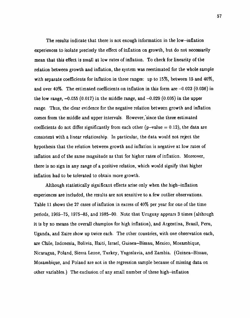
57
The results indicate that there is not enough information in the low-inflation
experiences to isolate precisely the effect of inflation on growth, but do not necessarily
mean that this effect is small at low rates of itiation. To check for linearity of the
relation between growth and inflation, the system was reestimated for the whole sample
with separate coefficients for inflation in three ranges: up to 15Y0,between 15 and 4070,
and over 4070. The estimated coefficients on inflation in this form are -0.023 (0.036) in
the low range, 4.055 (0.017) in the middle range, and -0.029 (0.005) in the upper
range. Thus, the clear evidence for the negative relation between growth and itiation
comes from the middle and upper intervals. However,’since the three estimated
coefficients do not differ significantly from each other (P-value = O.12), the data are
consistent with a linear relationship. In particular, the data wotid not reject the
hypothesis that the relation between growth and inflation is negative at low rates of
inflation and of the same magnitude as that for higher rates of inflation. Moreover,
there is no sign in any range of a positive relation, which would signify that higher
inflation had to be tolerated to obtain more growth.
Although statistically significant effects arise only when the high–inflation
experiences are included, the restits are not sensitive to a few outlier observations.
Table 11 shows the 27 cases of inflation in excess of 40% per year for one of the time
periods, 1965–75, 1975-85, and 1985–90. Note that Uruguay appears 3 times (although
it is by no means the overall champion for high inflation), and Argentina, Brazil, Peru,
Uganda, and Zaire show up twice each. The other countries, with one observation each,
are Chile, Indonesia, Bolivia, Haiti, Israel, Guinea-Bissau, Mexico, Mozambique,
Nicaragua, Poland, Sierra Leone, Turkey, Yugoslavia, and Zambia. (Guinea–Bissau,
Mozambique, and Poland are not in the regression sample because of missing data on
other variables. ) The exclusion of any small number of these high–inflation

58
observations —Nicaragua and Zaire were suggested by Bruno and Easterly (1995)—has
a negligible effect on the results.
The estimates are also reasonably stable over time. If different coefficients for
i~ation are allowed for each period, but the system is otherwise the same as in
column 1 of Table 10, then the resulting estimates are -t).040 (0.015) for 1965-75,
-0.040 (0.010) for 1975-85, and +.026 (0.005) for 1985-90. These values do not differ
significantly from each other (P-value = 0.29).
The standard deviation of inflation can be added to the system to see whether
itiation vanability has a relation with growth when the average inflation rate is held
constant. The strong positive correlation bet ween the mean and vanabilit y of inflation
(Figure 15) suggests that it would be difficult to distinguish the influences of these two
aspects of inflation. Howeverj when the two variables are entered jointly into the
regression system in column 2 of Table 10, the estimated coefficient on inflation remains
similar to that found before (-0.032 [0.008]), and the estimated coefficient on the
standard deviation of inflation is essentially zero (0,003 [0.009]).38 Thus, for a given
average rate of inflation, the variability of inflation has no significant relation with
growth. One possible interpretation of this result is that the realized variability of
inflation does not adequately measure the uncertainty of inflation, the van able that one
would have expected to be negatively related to growth. This issue is worth further
investigation.
C. The Endogeneity of Inflation
The key problem in interpreting the effect of inflation on growth from column 1 of
38This system includes on the right–hand side standard deviations of inflation measured forthe periods 1965–75, 1975-85, and 1985–90. These variables are also included with theinstruments. The findings are similar if longer term measures of the standard deviation areused instead of the cent emporaneous values.

59
Table 10 is that the regression need not reflect causation from inflation to growth.
Inflation is an endogenous vanable, which may respond to growth or to other variables
that are related to growth. For example, an inverse relation between growth and
inflation would arise if an exogenous slowing of the growth rate tended to generate
higher inflation. This increase in inflation could result if monetary authorities reacted
to economic slowdowns with expansionary policies. Moreover, if the path of monetary
aggregates did not change, then the equality between money supply and demand at each
point in time implies that a reduction in the growth rate of output would tend
automatically to raise the inflation rate.
Kocherlakota (1996) focused on this last source of endogeneity bias. To fix ideas,
suppose as he does that the money growth rate, At, is determined exogenously. The
relation bet ween the inflation rate, ~t, and pt is given from the money+upply~quals-
moneydemand condition by
(3) Tt=pt–gt+vt)
where gt is the growth rate of output and Vt is an independent shock to velocity.
Suppose that the effect of inflation on the growth rate is described by
(4)
where Et is an independent shock and a is the coefficient to be estimated..
In this framework, the OLS regression coefficient, a, of gt on mt can be shown to
be given by
(5).
{ VAR,(P)VAR(‘JAR(~. [VAR~=– +VAR(V +VAR(Cp)+ v)+ ‘)t) “
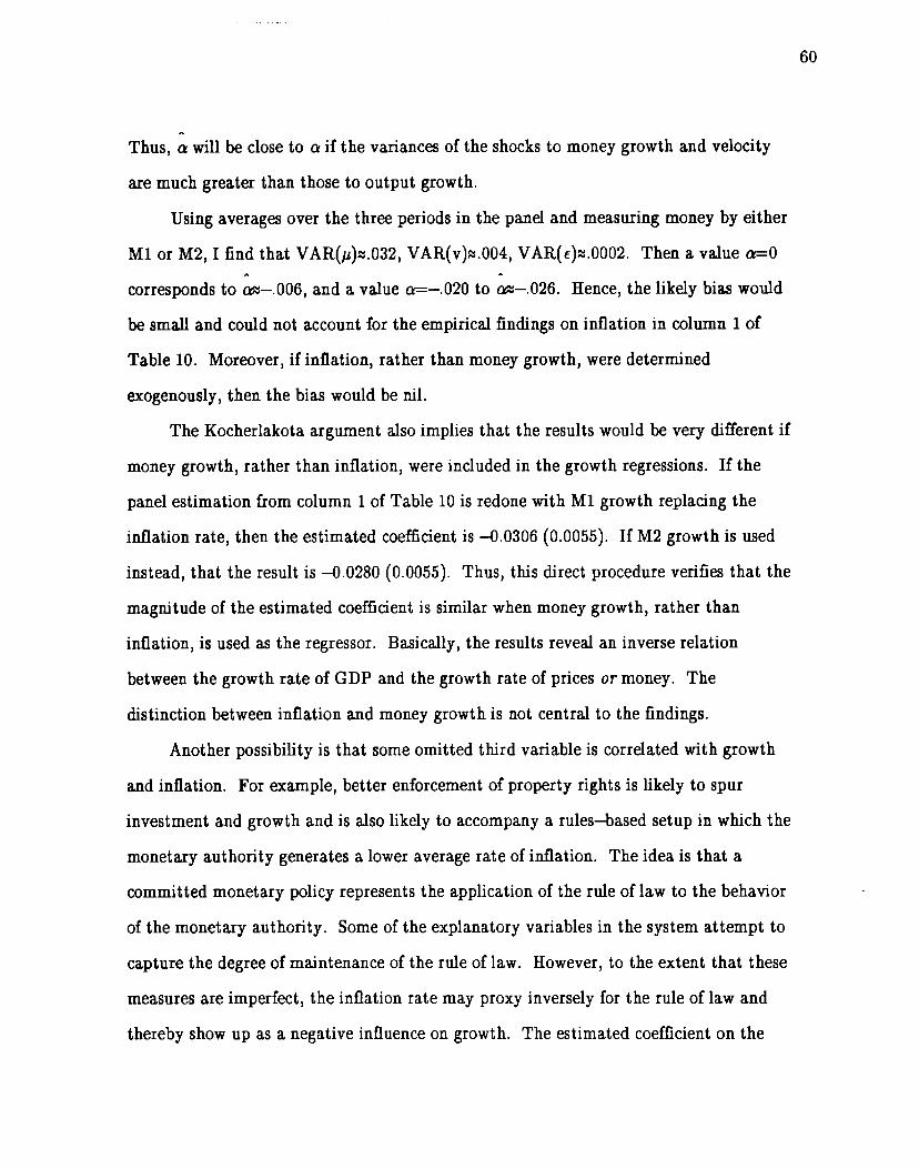
60
.
Thus, atillbclose toaifthe vtiances of theshocks tomoney growth ad velocity
are much greater than those to output growth.
Using averages over the three periods in the panel and measuring money by either
Mlor M2, Ifindthat VAR(~)x.032) VAR(v)&.004, VAR(~)x.OOO2. Then avalue_O. .
corresponds to m–.006, and a value -–.020 to w–.O26. Hence, the likely bias would
be small and could not account for the empirical findings on inflation in mlumn 1 of
Table 10. Moreover, if inflation, rather than money growth, were determined
exogenously, then the bias would be nil.
The Kocherlakota argument also implies that the results would be very different if
money growth, rather than inflation, were included in the growth regressions. If the
panel estimation from column 1 of Table 10 is redone with Ml growth replacing the
itiation rate, then the estimated coefficient is -0.0306 (0.0055). If M2 growth is used
instead, that the result is -0.0280 (0.0055). Thus, this direct procedure verifies that the
magnitude of the estimated coefficient is similar when money growth, rather than
inflation, is used as the regressor. Basically, the results reveal an inverse relation
bet ween the growth rate of GDP and the growth rate of prices or money. The
distinction between inflation and money growth is not central to the findings.
Another possibility is that some omitted third variable is correlated with growth
and inflation. For example, better enforcement of property rights is likely to spur
investment and growth and is also likely to accompany a rules-based setup in which the
monetary authority generates a lower average rate of inflation. The idea is that a
committed monetary policy represents the application of the rule of law to the behavior
of the monetary authority. Some of the explanatory variables in the system attempt to
capture the degree of maintenance of the rde of law. However, to the extent that these
measures are imperfect, the inflation rate may proxy inversely for the rule of law and
thereby show up as a negative influence on growth. The estimated coefficient on the

61
inflation rate could therefore reflect an effect on growth that has nothing to do with
inflation, per se.
Some researchers like to handle this type of problem, as discussed in the first
essay, by using some variant of fixed-effects estimation; that is, by allowing for an
individual constant for each country. This procedure basic~y eliminates
cross-sectional information about inflation from the sample and therefore relies on
effects within countries from changes over time of inflation and other variables. It is not
appaent that problems of correlation of inflation with omitted variables wotid be less
serious in this time-series context than in cross sections. (If a country is undergoing an
inflation crisis or implementing a monetary reform, then it is likely to be experiencing
other crises or reforms at the same time. ) Moreover, the problems with measurement
error and timing of relationships would be more substantial in the time series. The one
thing that is clear is that fixed-effects procedures lose a lot of information.
Another way to proceed is to find satisfactory instrumental variables-reasonably
exogenous variables that are themselves significantly related to inflation. My search
along these lines proceeded along the sequence now described.
1. Central Bank Independace
One promising source of instruments for inflation involves legal provisions that
guarantee more or less central bank independence. A recent literature (Bade and Parhn
[1982]; Grilli, Masciandaro, and Tabellini [1991]; Cukerman [1992]; and Alesina and
Summers [1993]) argues that a greater degree of independence leads to lower average
rates of money growth and inflation and to greater monetuy stability. The idea is that
independence enhances the ability of the central bank to commit to price stability and,
hence, to deliver low and stable inflation. (This view assumes that central bankers have
relatively strong preferences for low inflation. ) Alesina and Summers (1993,

62
Figures la, lb) find striking negative relationships among 16 developed countries from
1955 to 1988 between an index of the degree of central bwk independence and the mean
and variance of inflation. Thus, in their context, the memure of central bank
independence satisfies one condition needed for a good inflation instrument; it has
substantial explanatory power for idation.
Because of the difficulty of enacting changes in laws, it is plausible that a good
deal of the cross-country differences in legal provisions that influence central bank
independence can be treated as exogenous. Problems arise, however, if the legrd
framework changes in response to inflation (although the sign of this interaction is
unclear). In addition, exogeneit y would be violated if alterations in a country’s legal
environment for monetary policy are correlated with changes in unmeasured
institutional featuresauch as structures that maintain property rights—that influence
growth rates. This problem is, however, mitigated by the inclusion of other explanatory
variables, notably the index of the rule of law, in the regression framework.
Cukierman (1992, Chapter 19) argues that the legal provisions that govern central
bank action differ substantially from the way that the banks actually operate. In
partictiar, he distinguishes the legal term of office of the central bank governor from the
observed turnover. The latter variable would be more closely related to bank
performance (and, hence, to inflation), but cannot be treated as exogenous to growth or
omitted t bird variables. Thus, for the purpose of constructing instruments for inflation,
the preferred strategy is to focus on the extent to which inflation can be explained by
differences in legal provisions for the central bank.
Table 12 shows an index of central bank independence for 67 countries, based on
the information compiled by Cukierman (1992, Chapter 19, Appendix A) over time
periods that correspond roughly to the four decades from the 1950s to the 1980s. The
index is an average over the time periods and for numerous categories of legal provisions

63
contained in the charters of the central banks; see the notes to the table. The details of
construction differ somewhat from those used by Cukierman, but the values shown in
the table are similar to those reported in his Table 19.3 for the 1980s.
Table 12 also conttins the average itiation rate from 1960 to 1990 for the 67
countries in my sample that have data on the index of central bank independence. A
mmparison between the index and the inflation rate reveals a crucial problem; the
correlation bet ween the two variables is essentially zero, as is clear from Figure 17. This
verdict is also maintained if one looks separately over the three decades from the 1960s
to the 1980s and if one holds constant other possible determinants of inflation. In this
broad sample of countries, differences in legal provisions that ought to affect central
bank independence have no explanatory power for inflation. 39
The Alesina–Summers (1993) finding of a close negative link between inflation and
central bank independence turns out to be a fragile one. In their sample of 16 developed
countries, the correlation between average inflation (between 1960 and 1990) and their
measure of independence is -0.82. If one ret tins their sample but switches to the
presumably more accurate indicator of independence based on Cukierman’s (1992)
information, then the correlation falls in magnitude to -0.59. If one sticks to developed
countries but enlarges the sample to the 23 OECD countries for which Cukierman had
data on independence, then the size of the correlation declines further to -0.18. (Iceland
is particularly troublesome in t Ms sample. ) Finally, if one considers the full sample of
67 countries with data (as in Figure 17), then the correlation becomes a negligible -0.02.
This negative finding about the role of central bank independence is of
considerable int crest, because it suggests that low inflation cannot be atttined merely by
instituting legal changes that appear to promote a more independent central bank.
s’JCukierman’s (1992, Chapter 20) results concur with this finding, especially for samples thatgo beyond a small number of developed countries, the kind of sample used in most of theliterature on central bank independence.

64
However, the result also means that we have to search further for instruments to clarify
the relation bet ween growth and inflation. AO
2. Lagged Intlation
Earlier values of a country’s inflation rate have substantial explanatory power for
inflation. A1 Lagged inflation would also be exogenous with respect to innovations in
subsequent growth rates. Hence, if lagged inflation is used as an instrument, then the
estimated relation between growth and inflation would not tend to rdect the short–run
reverse effect of growth on inflation.
One problem, however, is that lagged inflation would reflect persistent
characteristics of a country’s monetary institutions (such as the extent to which
policymakers have credibilityy), and these characteristics could be correlated with
omitted variables that are relevant to growth (such w the extent to which political
institutions support the maintenance of property rights). The use of lagged inflation as
an instrument would therefore not rule out the problems of interpretation that derive
from omitted third variables. However, the inclusion of the other explanatory variables
in the regression framework lessens this problem. Another favorable element is that the
residuals from the growth equations are not significantly correlated over the time
periods.
40cukierman, et ~ (1993) use as instruments the turnover rate of bank governors and theaverage number of changes in bank leadership that occur within six months of a change ingovernment. These measures of actual bank independence have substantial explanatorypower for inflation but would not tend to be exogenous with respect to growth.
411have carried out SUR estimation of a panel system with the inflation rate = thedependent variable (for 1965–75, 1975-85, and 1985–90), where the independent variablesare lagged inflation and its square and the instrumental variables other thancontemporaneous inflation used in column 1 of Table 10. The estimated coefficient oflagged inflation is 1.47 (0.10) and that on its square is –1.01 (.09). No other estimated
ncoefficients are significant at the 107ocritical level. The R’ values for the three periods are0.60, 0.39, and 0.20.

65
Column 3 of Table 10 shows the estimated effect of inflation on the growth rate
when lagged inflation (over the five years prior to each sample period) and its square are
used as instruments. The estimated coefficient is -0.026 (0.005), slightly smaller in
magnitude than that found in column 1 when contemporaneous inflation is included as
an inst rurnent. Thus, it seems that most of the estimated negative relation between
growth and inflation does not represent reverse short–term (negative) effects of growth
on inflation.
The significant negative influence of inflation on growth still shows up only when
the high–inflation observations are included. The results are, however, again consistent
with a linear relation and with stability over the time periods. The standard deviation
of inflation also remains insignificant if it is added to the regressions (column 4 of
Table 10).
3. Prior Colonial Status
Another possible instrument for inflation comes from the observation that prior
colonial status has substantial explanatory power for inflation. Table 13 breaks down
averages of inflation rates from 1960 to 1990 by groups of countries classified, as in the
second essay, as non-colonies and former colonies of Britain, France, Spain or Portugal,
and other countries (in this sample, Australia, Belgium, the Netherlands, New Zealand,
and the United States).
Table 13 indicates that the average inflation rate for all 117 countries from 1960 to
1990 was 12.6% per year. The average for the 30 non<olonies of 8.9% was similar to
that of 10.4% for the 42 British colonies and 6.6% for the 20 French colonies. However,
the rates were strikingly higher for the 18 Spanish or Portuguese colonies-29.4%-and
somewhat higher for the 7 other colonies—16. lYo.

66
A key reason for the low average itiation rate in the former French colonies is the
participation of most of the Sub Saharan African states in the fixed-exchange rate
regime oft he CFA Franc. Aa This type of reasonabl y exogenous commitment to
relatively low inflation is exactly the kind of experiment that provides for a good
instrument for inflation.
For many of the former British colonies, a significant element may be their prior
experience with British organized currency boards, another system that tends to
generate low inflation (see Schwartz [1993]). These boards involved, at one time or
another before independence, most of the British colonies in Africa, the Caribbean,
southeast Asia, and the mideast.
The high average inflation rate for the 16 former Spanish colonies in the sample
does not reflect, per se, their presence in Latin America. For seven Latin American
countries that are not former Spanish or Portuguese colonies, Aqthe average inflation rate
for 1960–90 was only 9.0%, virtually the same as that for the non-colonies (see
Table 13). Also, four former Portuguese colonies in Africa experienced the relatively
high average inflation rate of around 20%.AAFor Portugal and Spain themselves, the
AzFordiscussions of the CFA Franc zone, see Boughton (1991) and Clement (1994). Thezone mtinttined a fixed exchange rate with the French Franc for 45 years until thedevaluation from 50 to 100 CFA Francs per French Franc in January 1994. At the time ofthe devaluation, the zone covered 14 African countries grouped around three central banks:the West African Monetary Union of Benin, Burkina Faso, Ivory Coast, Mali, Niger,Senegal, and Togo; a group of central African countries consisting of Cameroon, CentralAfrican Republic, Chad, Congo, Equatorial Guinea, and Gabon; and the Comoros. Someoriginal members of the zone left to establish independent currencies—Djbouti in 1949,Guinea in 1958, Mali in 1962 (until it rejoined in 1984), Madagascar in 1963, Mauritania in1973, and the Comoros in 1981 (to set up its own form of CFA franc). Equatorial Guinea,which joined in 1985, is the ordy member that is not a former colony of France (and notFrench~peaking).
AoTheseven in the sample are Barbados, Dominican Republic (attributed to France ratherthan Spain; see the notes to Table 13), Guyana, Htiti, Jamaica, Suriname, and Trinidad &Tobago. Five other former British colonies in Latin America that are not in thissampleBahamas, Belize, Grenada, St. Lucia, and St. Vincent-xpenenced therelatively low average inflation rate of 6.970 horn 1970 to 1990.
AAThesefour are Angola, Cape Verde, Guinea-Bissau, and Mozambique. Data are

67
average inflation rate of 10.9~0 for 1960–90 was well below the rate of 29.4% experienced
by their former colonies. However, 10.9% inflation was substantially higher than that
experienced by France (6.4%) and the United Kingdom (7.7%).
The regression
Table l~hows the
instruments exclude
system focused on in the first essay=hown in column 1 of
estimated effect of inflation on the growth rate of GDP when the
contemporaneous or lagged inflation but include indicators of prior
colonird status. The two variables used are a dummy for whether the country is a
former Spanish or Portuguese colony and a dummy for whether the country is a former
colony of a country other than Brittin, France, Sptin, or Portugal. ASThe estimated
coefficient on the inflation rate is now -0.043 (0.008), higher in magnitude than that
found in Table 10 when contemporaneous or lagged inflation is used as an instrument.
The significantly negative relation between growth and inflation again arises ordy when
the high–inflation experiences are included in the sample. The results dso continue to
be stable over the time periods.
One question about the procedure is whether prior colonial status works in the
growth regressions only because it serves as an imperfect proxy for Latin America, a
region that is known to have experienced surprisingly weak economic growth (see, for
example, the results in Barro [1991]). However, column 2 of Table 1 showed that if a
unavailable for Cape Verde and Guinea-Bissau in the 1960s (prior to independence). Thefigures for Angola in the 1980s me rough estimates.
A51have carried out SUR estimation of a panel system with the inflation rate as thedependent variable (for 1965–75, 1975-85, and 1985–90), where the independent variablesare the instrumental variables used in column 1 of Table 1. The estimated coefficient onthe Spain–Portugal colonial dummy is 0.125 (0.027) and that on the dummy for other
dcolonies is 0.159 (0.051 . The R2 values are 0.35 for 1965–75, 0.09 for 1975-85, and 0.05for 1985–90. Thus, in ation is difficult to explain, especially if most contemporaneousvariables and lagged inflation are excluded as regressors (see n. 40). Two variables that aresometimes suggested as determinants of inflation-trade openness (measured by ratios ofexports and imports to GDP) and country size (measured by log of population —areinsignificant if added to the system. 1Years since independence also has no exp anatorypower for inflation. This result may arise because the former colonies of Spain andPortugal in Latin America became independent at rougMy the same time.

68
dummy variable for Latin America is included in the system (along with dummies for
Sub Saharan Africa and East Asia), then the estimated coefficient of inflation changes
little: +.039 (0.008). Moreover, the estimated coefficient on the Latin America
dummy is not statistically significant at conventional levels, +.0054 (0.0032). The
resdts are basicaJ.ly the same if the Latin America dummy is added to the system from
column 1 of Table 10, in which contemporaneous inflation is used as an instrument. It
therefore appears that much of the estimated effect of a Latin America dummy on
growth rates in previous research reflected a proxying of this dummy for high inflation.
In partictiar, the negative effect of inflation on growth does not just reflect the tendency
of many high-inflation countries to be in Latin America.
D. S~ Findings on Inflation
A major result is that the estimated effect of inflation on growth is significantly
negative when some plausible instruments are used in the statistical procedures. Thus,
there is some reason to believe that the relations reflect causation from higher long–term
itiation to reduced growth.
It should be stressed that the clear evidence for adverse effects of inflation comes
from the experiences of high inflation. The magnitudes of effects are dso not that large;
for example, an increase in the average inflation rate by 10 percentage points per year is
estimated to lower the growth rate of real per capita GDP on impact by 0.3-0.4
percentage points per year.
Some people have reacted to these kinds of findings by expressing skepticism about
the value of cross-country empirical work. In fact, the wide differences in inflation
experiences offered by this kind of panel provide the best opportunity for ascertaining
the long–term effects of inflation and other variables on economic performance. If the
effects cannot be detected accurately with these data, then they probably cannot be

pinpointed anywhere else. In particular, the usual focus on annual or quarterly time
series of 3H0 years for one or a few countries is much less promising.
In any event, the apparently small estimated effects of inflation on growth are
misleading. Over long periods, these changes in growth rates have dramatic effects on
standards of living. For example, a reduction in the growth rate by 0.3+.4 percentage
points per year (produced on impact by 10 percentage points more of average inflation)
means that the level of real gross domestic product would be lowered after 30 years by
6–9%. AdIn 1995, the U.S. gross domestic product was around $7–1/2 trillion; 6–9% of
this amount is $450+80 billion, more than enough to justify a keen interest in price
stability.
AdInthe model, the fall in the growth rate by 0.3-0.4 percent per year apphes on impact inresponse to a permanent increase in the inflation rate. The growth rate would alsodecrease for a long time thereafter, but the ma nitude of this decrease diminishes toward
%mro as the economy converges back to its (uric anged) long–run growth rate, Hence, inthe very long run, the effect of higher inflation is a path with a permanently lower level ofoutput, not a reduced growth rate. The numerical estimates for the reduced level of outputafter 30 years take account of these dynamic effects. The calculation depends on theeconomy’s rate of convergence to its long–term growth rate (assumed, based on theempincd estimates, to be 2–3 percent per year). Also, the computations unrealisticallyneglect any responses of the other explanatory variables, such as the human-capitalmeasures and the fertility rate.
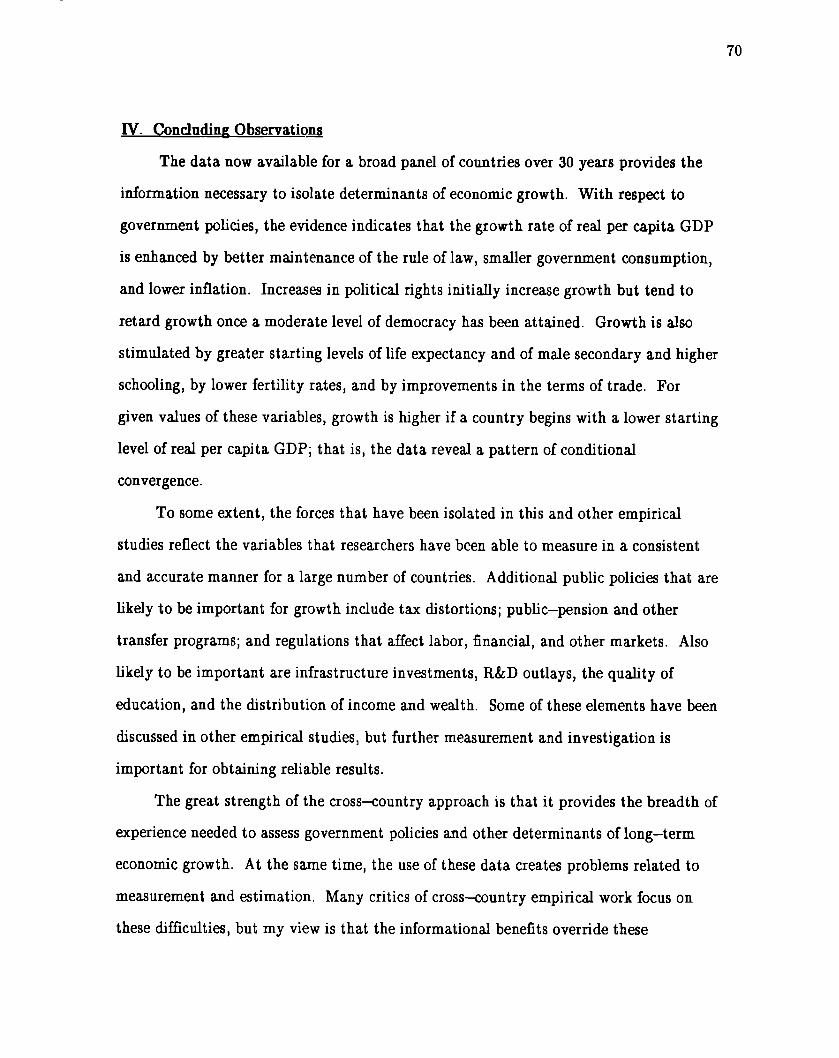
70
w. co ncludin~ Observatio~
The data now available for a broad panel of countries over 30 years provides the
information necessary to isolate determinants of economic growth. With respect to
government policies, the evidence indicates that the growth rate of real per capita GDP
is enhanced by better maintenance of the rule of law, smaller government consumption,
and lower inflation. Increases in political rights initi~y increase growth but tend to
retard growth once a moderate level of democracy has been attained. Growth is also
stimulated by greater starting levels of life expectancy and of male secondary and higher
schooling, by lower fertility rates, and by improvements in the terms of trade. For
given values of these variables, growth is higher if a country begins with a lower starting
level of real per capita GDP; that is, the data reveal a pattern of condition
convergence.
To some extent, the forces that have been isolated in this and other empirical
studies reflect the variables that researchers have been able to measure in a consistent
and accurate manner for a large number of countries. Additional public policies that are
likely to be important for growth include tax distortions; public-pension and other
transfer programs; and regulations that affect labor, financial, and other markets. Also
likely to be important are infrastructure investments, R&D outlays, the qualit y of
education, and the distribution of income and wealth. Some of these elements have been
discussed in other empirical studies, but further measurement and investigation is
important for obtaining reliable results.
The great strength of the cross-country approach is that it provides the breadth of
experience needed to assess government policies and other determinants of long–term
economic growth. At the same time, the use of these data creates problems related to
measurement and estimation. Many critics of cross-country empincd work focus on
these difficulties, but my view is that the informational benefits override these

71
objections. Naturally, this viewpoint will become more persuasive if futher progress can
made in overmming the problems of measurement and estimation.
72
References
Aghion, Philippe and Peter Hewitt (1992). “A Model of Growth through Creative
Destruction,” Economettica, 60, 2 (Much), 323–351.
Alesina, Alberto ad Enrico Spolaore (1995). “On the Number and Size of Nations,”
unpublished, Harvard University, October.
Alesina, Alberto and Lawrence H. Summers (1993). “Central Bank Independence and
Macroeconomic Performance: Some Comparative Evidence, ” Journal oj Mouy,
Credit, and Banking, 25 (May), 151–162.
Aristotle (1932). Politics, translated by H. Rackham, Cambridge MA, Harvard
University Press.
Arrow, Kenneth J. (1962). “The Economic Implications of Learning by Doing,” Retiew
of Economic Studies, 29 (June), 155–173.
Bade, Robin and J. Michael Parkin (1982). “Central Bank Laws and Monetary Policy,”
unpublished paper, University of Western Ontario.
Barrett, David B., editor (1982). World Chfitian Encyclopedia, Oxford, Oxford
University Press.
Barre, Robert J. (1991). “Economic Growth in a Cross Section of Countries,” Quarterly
Journa/ of Economics, 106, 2 (May), 407433.
Barre, Robert J. and Jong–Wha Lee (1993). “International Comparisons of
Educational Attainment ,“ Journal of Monetary Economics, 32 (December),
363–394.
Barre, Robert J. and Jong–Wha Lee (1994). “Sources of Economic Growth,” Carnegie-
Rochester Conference Series on Public Policy (June), 146.
Barre, Robert J. and Xavier Sala–i-Martin (1995a). Economic Growth, New York,
McGraw Hill.

73
Barre, Robert J. and Xavier Sda-i-Martin (1995b). “Technological Diffusion,
Convergent, and Growth,” National Bureau of Emnomic Research, working paper
no. 5151, June.
Becker, Gary S. and ~bert J. Barro (1988). “A Reformtiation of the Economic Theory
of Fertilit y,” Quatierly Journal of Economics, 103, 1 (February), 1–25.
Behrman, Jere R. (1990). “Women’s Schooling and Nonmarket Productivity y: A Survey
and a Reappraisal, ” unpublished paper, University of Pennsylvtia.
Benhabib, Jess and Mark M. Spiegel (1994). “The Role of Human Capital in Ewnomic
Development: Evidence from Aggregate Crosscountry Data,” Journal of
Moneta~ Economics, 34, 2 (October), 143–173.
Blomstrom, Magnus, Robert E. Lipsey, and Mano Zejan (1993). “Is Fixed Investment
the Key to Economic Growth?,” National Bureau of Economic Research working
paper no. 4436, August.
Bollen, Kenneth A. (1990). “Political Democracy: Conceptual and Measurement
Traps,” Studies in Comparative International Development, Spring, 7–24.
Boughton, James M. (1991). “The CFA Franc Zone: Currency Union and Monetary
Standard,” International Monetary Fund, working paper no. 91/133 (forthcoming
in Anthony Courakis and George Tavlas, eds., Monetary Integration, Cambridge,
Cambridge University Press).
Briault, Clive (1995). “The Costs of Inflation,” Bank of England Quarterly Bulletin, 35,
February, 33-15.
Bruno, Michael and William Easterly (1995). “Inflation Crises and Long–Run
Growth,” National Bureau of Economic Research, working paper no. 5209, August.
Caballe, Jordi and Manuel S. Smtos (1993). “On Endogenous Growth with Physical
and Human Capita l,” Journal of Political Economy, 101, 6 (December),
1042–1067.

74
Caselli, Francesco, Gerardo Esquivel, and Fernando Lefort (1995). “Reopening the
Convergent Debate: A New Look at Cross-Country Growth Empirics,”
unpublished paper, Harvard University, November.
Cass, David (1965). “Optimum Growth in an Aggregative Model of Capital
Accumulation,” Retiew of Economic Studies, 32 (July), 233–240.
Clement, Jean A.P. (1994). “Striving for Stability: CFA Franc Realignment,”
Finance & Development, June, 10-13.
Cu.kierma, Ala (1992). Central Bank Strategy, Credibility, and Independence, MIT
Press, Cambridge MA.
Cukierman, Alex, Pantelis Kalaitzidakis, Lawrence H. Summers, and Steven B. Webb
(1993). “Central Bank Independence, Growth, Investment, and Real Rates,”
Came~e-Rochester Conference Seties on Public Policy, 39, 95–140.
DeLong, J. Bradford and Lawrence H. Summers (1991). “Equipment Investment and
Economic Growth,” Quarterly Journal ojEconornics, 106, 2 (May), 445-502.
Fischer, Stardey (1993). “The Role of Macroeconomic Factors in Growth,” Journal of
Moneiaq Economics, 32, 3 (December), 485–512.
Friedman, Milton (1962). Capitaltim and Freedom, Chicago, University of Chicago
Press.
Galton, Francis (1886). “Regression towards Mediocrity in Hereditary Stature,”
JoumaL of the Anthropolo@cal Institute of Great Btitain and Ireland, 15, 246–263.
Gdton, Frmcis (1889). Natural Inheritance, London, Macmillan.
Gastil, Raymond D. and followers (1982+3 and other years). Freedom in the World,
Westport CT, Greenwood Press.
Gastil, Raymond D. (1991), “The Comparative Survey of Freedom: Experiences and
Suggestions, ” in Alex Inkeles, ed., On Measuring Democracy, New Brunswick NJ,
Trmsaction Publishers.
75
Gner, Kevin B. and Gordon Tdlock (1989). “An Empirical Analysis of Cross–National
Economic Growth,” Journal of Monetaw Economics, 24, 2 (September), 259–276.
Grilli, Vittorio, Donato Mwciandaro, and Guido Tabellini (1991). “Political ad
Monetary Institutions and Public Finance Policies in the Industrial Countries,”
Economic Po/icv, 13 (October), 341–392.
Grossman, Gene M. and Elhanan Helpman (1991). Innovation and Grozuth in the GZobal
Economy, Cambridge MA, MIT Press.
Hart, Peter E. (1995). “Galtonian Regression Across Countries and the Convergence of
Productivity y,” Oz~ord Bul/etin of Economics and Stattitics, 57,3 (August),
287–293.
Helliwell, John F. (1994). “Empirical Linkages Between Democracy and Economic
Growth,” British Journal of Political Science, 24, 225–248.
Huber, Evelyne, Dietnch Rueschemeyer, and John D. Stephens (1993). “The Impact of
Economic Development on Democracy,” Journal of Economic Perspectives, 7,
Summer, 71-85.
Huntington, Samuel P. (1991). The Third Wave: Democrattiation in the Late
Twentieth Century, Norman, Oklahoma, University of Oklahoma Press.
Inkeles, Alex (1991). On Measuting Democra~, New Brunswick NJ, Transaction
Publishers.
Islam, N=rul (1995). “Growth Empirics: A Panel Data Approach,” Quarterly Journal
of Economics, 110, 4 (November), 1127–1 170.
Jain, S. (1975). Size Dtittibution of Income: A Compdation of Data, Washington DC,
The World Bank.
Knack, Stephen and Philip Keefer (1995). “Institutions and Economic Performance:
Cross-Country Tests Using Alternative Institutional Measures,” Economics and
Politics, 7, 207–227.

76
Knight, Frank H. (1944). “Diminishing Returns from Investment ,“ Journal of Political
EcOnOm~,52 (March), 26-47.
Knight, Malcolm, Norman Loayza, and Delano ViUanueva (1993). “Testing the
Neoclassical Theory of Economic Growth,” IMF Staff Papers, 40, 3 (September),
512–541.
Kocherlakota, N.R. (1996). “Discussion of Inflation and Growth,” in Federal Reserve
Bank of St. Louis, Price Stability and Economic Growth.
Koopmans, Tjalling C. (1965). “On the Concept of Optimal Economic Growth,” in The
Econometric Approach to Development Planning, Amsterdam, North Holland.
Kormendi, Roger C. and Philip G. Megu.ire (1985). “Macroeconomic Determinants of
Growth,” Journal of Moneta~ Economics, 16, 2 (September), 141–163.
Lecaillon, Jacques, et al (1984), Income Dtittibution and Economic Development,
Geneva, International Labor Office.
Lipset, Seymour Martin (1959). “Some Social Requisites of Democracy: Economic
Development and Political Legitimacy,” American Political Science Review, 53,
69-105.
Lipset, Seymour Martin (1994). “The Social Requisites of Democracy Revisitedj”
Ametican Sociological Retiew, 59 (February), 1–22.
Lipset, Seymour Martin, Kyoung–Ryung Seong, and John Charles Torres (1993). “A
Comparative Analysis of the Social Requisites of Democracy,” International Social
Science Journal (May), 155-175.
Logue, Dennis E. and Thomas D. Willett (1976). “A Note on the Relationship between
the Rate and Variability of Inflation,” Economics, 43, 151–158.
LUCM,Robert E., Jr. (1988). “On the Mechanics of Economic Development ,“ Journa/ of
Moneta~ Economics, 22, 1 (July), 3A2.

77
Malthus, Thomas R. (1798). An Essay on tie Principle of Population, London, W.
Pickering, 1986.
Mankiw, N. Gregory, David Romer, and David N. Weil (1992). “A Contribution to the
Empirics of Economic Growth,” Quarterly Journal of Economics, 107, 2 (May),
407437.
Mauro, PW1O(1995). “Corruption, Country Risk, and Growth,” @arterly Jouti of
Economics, 110 (October).
Mtiigan, Casey B. and Xavier Sala-i-Martin (1993). “Transitional Dynamics in
Tw~Sector Models of Endogenous Growth,” Quarterly Journal of Economics, 108,
3 (August), 737–773.
Nelson, Richard R. and Edmund S. Phelps (1966). “Investment in Humans,
Technological Diffusion, and Economic Growth,” American Economic Retiew, 56,
2 (May), 69–75.
Okun, Arthur M. (1971). “The Mirage of Steady Inflation,” Broo~ngs Papers on
Economic Activity, 2, 485-498.
Perotti, Roberto (1996). “Growth, Income Distribution, and Democracy,” Journal oj
Economic Growth, 1, 2 (June).
Przeworski, Adam and Fernando Limongi (1993). “Political Regimes and Economic
Growth,” Journal of Economic Perspectives, 7, Summer, 51-69.
Putnam, Robert D., with Robert Leonardi and Raffaella Y. Nanetti (1993). Mafing
Democracy Work, Civic Traditiom in Modern Italy, Princeton NJ, Princeton
University Press.
Quah, Danny (1993). “Galton’s Fallacy and Tests of the Convergence Hypoth~is,”
Scandinavian Journal of Economics, 95,4 (December), 427443.
Ramsey, Frank (1928). “A Mathematical Theory of Saving,” Economic Journal, 38
(December), 543-559.

78
Wbelo, Sergio (1991). “Long-Run Policy Analysis and Long–Run Growth,” Journal of
Po/itical Ecowmy, 99, 3 (June), 500-521.
Ricardo, David (1817). On the Ptincipks of Political Economy and Tuation, P. Sraffa,
cd., Cambridge, Cambridge University Press, 1951.
Romer, Paul M. (1986). “Increasing Returns and Long–Run Growth,” Joumd of
Political Economy, 94, 5 (October), 1002–1037.
Wmer, Paul M. (1987). “Growth Based on Increasing Returns Due to Specialization,”
American Economic Retiew, 77,2 (May), 56-62.
Miner, Paul M. (1990). “Endogenous Technological Change,” Joumai of Political
Economy, 98, 5 (October), part II, S71–S102.
Sachs, Jeffrey D. and Andrew M. Warner (1995). “Natural Resource Abundance and
Economic Growth,” unpublished, Harvard Institute for International
Devdopment, December.
Sah, Raaj K. (1991). “Fallibility in Human Organizations and Political Systems,”
Journal of Economic Perspectives, 5, Spring, 67-88.
Schultz, T. Paul (1989). “Returns to Women’s Education,” PHRWD background
paper 89/001, The World Bank, Poptiation, Health, and Nutrition Department,
Washington D.C.
Schurnpeter, Joseph A. (1934). The Z’heo~ of Economic Development, Cambridge MA,
Harvard University Press.
Schwartz, Anna J. (1993). “Currency Boards: Their Past, Present, and Possible Future
Mle,” Camegi+Rochegter Conference Serieg on Public Policy, 39, 147–187.
Schwarz, Gerhard (1992). “Democracy and Market-Oriented Reform—A Love-Hate
Relationship?,” Economic Education BuUetin, 32, 5 (May).

79
Sheshinski, Eytan (1967). “Optimal Accumulation with Learning by Doing)” in Karl
Shell, ed., Essays on the Z’heo~ of Optimal Economic Grotih, Cambridge MA,
MIT Press, 31-52.
Sirowy, L=ry and Alex Inkel~ (1990). “The Effects of Democracy on Economic
Growth and Inequality: a Review,” Studies in Comparative International
Development, 25, Spring, 126–157.
Solow, Robert M. (1956). “A Contribution to the Theory of Economic Growth,”
Quarterly Journal of Economics, 70, 1 (February), 65–94.
Summers, Robert and Alan Heston (1991). “The Penn World Table (Mark 5): An
Expanded Set of International Comparisons, 1950–1988,” Quarterly Journal of
Economics, 106, 2 (May), 327–368.
Summers, Robert and Alan Heston (1993). “Penn World Tables, Version 5.5,” available
on diskette from the National Bureau of Economic Research, Cambridge MA.
Swan, Trevor W. (1956). “Economic Growth and Capital Accumulation,” Economic
Record, 32 (November), 334–361.
Tocqueville, Altis de (1835). Democracy in Ametica, translated by Henry Reeve,
London, Saunders & Otley.
Uzawa, Hirofumi (1965). “Optimal Technical Change in an Aggregative Model of
Economic Growth,” lntemational Economic Retiew, 6 (January), 18–31.

6-20-96 Table 1 Regressions for Per Capita Growth late
independent variable
log(GDP)
male secondary ad higher schooling
log(life expectancy)
log(GDP)*male schooling
log(fertility rate)
government consumption ratio
rule-of-lau index
terms-of-trade change
democracy index
democracy index squared
inflation rate
Sub Saharan Africa dummy
Latin America dummy
East Asia dummy
R2
number of observations
(1)
-.0254(.0031)
.0118(.0025)
.0423(.0137)
-.0062(.0017)
-.0161( .0053)
-.136(.026)
.0293(.0054)
.137(.030)
.090*(.027)
-.088(.024)
-.043(.008)
--
--
--
.58, .52,.42
80, 87,84 “
(2)
-.0225( .0032)
.0098(.0025)
.0418(.0139)
-.0052(.0017)
-.0135( .0053)
-.115(.027)
.0262(.0055)
.127(.030)
.094(.027)
-.091(.024)
-.039(.008)
.0042**~.0043)
-.0054( .0032)
.0050(. 0041)
.60, .52,.47
80, 8784
*p-value for joint significance of two democracy variables is 0.0006 incolumn 1 ad 0.0004 in column 2.
**p-value for joint significance of three dummyvariables is 0.11.

Notes to Table 1: The system has three equations, uhere the dependentvariables are the growth rate of real per capita GDPfor 1965-75, 1975-85,and 1985-90. The variables GDP (real per capita gross domestic product) andmale schooling (years of attainment for the population aged 25 and over atthe secondary and higher levels) refer to 1965, 1975, and 1985. Lifeexpectancy at birth is for 1960-64, 1970-74, and 1980-84. The variablelog(GDP)*male schooling is the product of log(GDP (expressed as a deviation
tfrom the sample mean) and the male upper-level sc oolin variable (alsofexpressed as a deviation from the sample ❑ean). The ru e-of-law index
applies to the early 1980s (one observation for each country). The terms-of-trade variable is the routh rate over each period of the ratio of export toimport prices. fThe in lation rate is the grouth rate over each period of aconsumer price index
ior of the GDPdeflator in a few cases). The other
variables are measure as averages over each period. These variables are thelog of the total fertility rate, the ratio of government consumption(exclusive of defense md education
ito GDP, and the democracy index. Column
2 includes dummyvariables for Sub aharan Africa, Latin America, and EastAsia. Individual constats (not shown) are also estimated for each period.
Estimation is by three-stage least squares (uith different instrumentalvariables used for each equation). The instruments include the five-yearearlier value of 10 (GDP) (for example,
!for 1960 in the 1965-75 equation);
the actual values o the schooling, life-expectancy, rule-of-law, and terms-of-trade variables; and, in column 2, the three area dummyvariables.Additional instruments are earlier values of the other variables except theinflation rate. For example, the 1965-75 equation uses the averages of thefertility rate and the government- spendin ratio for 1960-64. Dummies for
!former colonies of Spain or Portugal and or former colonies of othercountries aside from Britain ad Frace are also included as instruments.(These variables have substantial explanatory power for inflation. ) Theinstrument list also includes the cross product of the lagged value oflog(GDP) (expressed as a deviation from the sample mean) with the ❑aleschooling variable (expressed as a deviation from the sample mean).
The estimation weights countries equally but allows for different errorvariances in each period and for correlation of these errors over time. Theestimated correlation of the errors for column 1 is -0.13 between the 1965-75and 1975-85 equations, 0.05 between the 1965-75 and 1985-90 equations, and0.04 between the 1975-85 and 1985-90 equations. The pattern is similar forcolumn 2. The estimates are virtually the same if the errors are assumed tobe independent over the time periods. Standard errors of the coefficient
estimates are shown in parentheses. The R2 values and numbers ofobservations apply to each period individually.

Table 2
Regressions for Investment Ratio
independent variable
log(GDP)
male secondary and higher schooling
log(life expectancy)
log(GDP)*male schooling
log(fertility rate)
government consumption ratio
rule-of-law index
terms-of-trade chmge
democracy index
democracy index squared
inflation rate
Sub Sahara Africa dummy
Latin America dummy
East Asia dummy
R2
number of observations
(1)
-.010(.011)
-.0032( .0088)
.259(.050)
-.0004(.0057)
-.0028(.0192)
-.264(.089)
.092(.023)
.074(.068)
.148(.069)
-.142(.061)
-.053(.022)
--
--
--
.59, .62,.61
80, 87,84 -
*p-value for joint significmce of three dummyvariables
(2)
-.005(.011)
-.0064( .0085)
.274(.051)
.0009(.0055)
.0056(.0186)
-.216(.087)
.074(.024)
.070(.064)
.168(.070)
-.153(.062)
-.036(.021)
.013*~.o19)
-.038(.014)
.010(.017)
.60, .65,.67
80, 8784
is 0.03.

Notes to Table 2: The systems correspond to those described in Table 1,except that the dependent variables are now the average ratios of real
iinvestment private plus public) to real GDPover the periods 1965-74,1975-84, an 1985-89. The correlation of the errors across the equations issubstantial in the systems for investment. For example, for column 1, thecorrelation between the first ad second periods is 0.53, that between thefirst and third periods is 0.35, and that between the second amd thirdperiods is 0.62.

Table 3 Results from First Differences and a Cross Section
independent variable
log(GDP)
male schooling
log(life expectancy)
log(GDP)*male schooling
log(fertility rate)
government consumption
rule-of-law index
terms-of-trade change
democracy index
democracy index squared
inflation rate
R2
number of observations
ratio
(1)
FirstDifference
-.0444( .0066)
-.0032(.0045)
-.0820(.0381)
.0052(. 0035)
-.0396(.0116)
.000(.048)
--
.102(.027)
.019(.029)
-.014(.026)
-.032(.005)
.29, .44
88, 91
(2)
CrossSection
-.0220(.0041)
.0141( .0030)
.0172(.0184)
-.0077(.0019)
-.0206( .0066)
-.114(.026)
.0294( .0066)
.078(.078)
.071(.026)
-.074(.023)
-.030(.006)
.76
80
(3)
Panel
-.0242(.0028)
.0123(.0023)
.0388(.0124)
-.0070(.0015)
-.0156(.0049)
-.110(.021)
.0300(.0051)
.129(.029)
.048(.019)
-.051(.016)
-.028(.004)
.56, .53.49
83 8884
(4)
p- value
.000
.68
.002
.18
.11
.024
--
.92
.51
.28
.12
Notes: The systems are variants of the one shown in COIW 1 of Table 1.Column 1 uses first differences of all variables and is estimated by the SURtechnique, uhich allous for a different error variance for the tuo periods andcorrelation of the errors across the periods. Column 2 uses means of allvariables and is estimated by OLS. Column 3 is the same as column 1 of Table 1,except that estimation is by SUR rather than three-sta e least squares.
fThe
p-values in column 4 refer to Vald tests of equality o the coefficients fromcolumns 1 ad 2.

Table 4
Winners and Losers for Prospective Economic Growth
Top 20 Prospects Bottom 20 Prospects
Country Predicted growth Country Predicted growthrate of real rate of real
per capita GDP per capita GDP1996-2000 1996-2000
(Z per year) (% per year)
South KoreaPhilippinesDominican Rep.IndiaPoland
PeruSri L*aMalaysiaArgentinaSingapore
ThailadGreeceChileParaguayHong Kong
GuyanaPakistanTaiwmEcuadorEgypt
Regional patterns:
6.25.65.45.35.2
5.25.0
::!4.6
4.64.64.34.24.2
4.23.93.83.83.8
all countries (86)Sub Saharan Africa (18)Latin America (22)
[]Asia 18OECD 21
2.40.52.93.72.4
Sierra LeoneSudantialawiBangladeshNiger
ZaireGambiaBotswanaSenegalPapua New Guinea
BrazilCongoAlgeriaZambiaHal i
NicaraguaCameroonTrinidadCosta RicaUgada
-3.6-2.7-0.2-0.2-0.1
-0.10.10.10.20.2
0.20.30.30.50.8
0.81.11.21.31.3

Regressions
dependent variable:
independent variable
constant
‘emOct-5
log(GDP)
male primary schooling
female primary schooling
log(life e~ectacy)
urbanization rate
log(population)
oil-country dummy
democt-10
E2
number of observations
for
Table 5
Democracy and Civil-Liberties Indexes
(1)
democracy
-0.91(0.26)
0.672
(0.028)
0.045(0.017)
-0.056(0.014)
0.060(0.014)
0.187(0.076)
-0.102(0.048)
0.0061(0.0043)
-0.107(0.030)
--
.59, .74, .66
.74, .76, .55
85, 97, 101102, 105, 102
(2)
democracy
-0.54(0.28)
0.650
(0.042)
0.041(0.019)
-0.047(0.015)
0.053(0.015)
0.100(0.085)
-0.061(0.051)
0.0049(0.0046)
-0.129(0.032)
0.035
(0.040)
.73, .67.75, .76, .57
89, 101102, 105, 102
(3)
civilliberties
-0.48(0.21)
0.680
(0.026)
0.037(0.014)
-0.037(0.011)
0.047(0.011)
0.096(0.062)
-0.032(0.039)
-0.0016(0.0035)
-0.101(0.025)
--
.59, .81, .77
.83, .70, .72
85, 97, 101102, 105, 102

Notes to Table 5
System (1) has six equations, where the dependent variables are thevalues of the Castil democracy index for 1972, 1975, 1980, 1985, 1990, and1994. The variable democt-5 is for 1965, 1972, and so on. (The data for
1965 are from Bollen [1990].) The variables GDP (real per-capita GDP), maleand female primary schooling (years of attainment for persons aged 15 andover at the primary level), urbanization rate, and population refer to 1965,1970, etc. Life expectacy at birth applies to 1960-64, 1965-69, and so on.The oil dummyequals 1 for countries designated as oil exporting by the IWand O otheruise. System (2) contains only the five equations that start withthe 1975 value of the democracy index. This system adds a second lag of theindex (applying to 1965, 1972, etc.) as m explmatory variable. System (3)is the same as system (1) except that the dependent variable and its lag arefor the Gastil civil-liberties index.
AThe value for 1965, from Bollen
[1990] , coincides with the democracy in ex. )
Each system contains only one constant, as shown. The estimation, by theSURtechnique, weights countries equally but allows for different errorvariances in each period and for correlation of these errors over theperiods. Standard errors of the estimated coefficients are shown in
parentheses. The R2 values apply to each period individually.
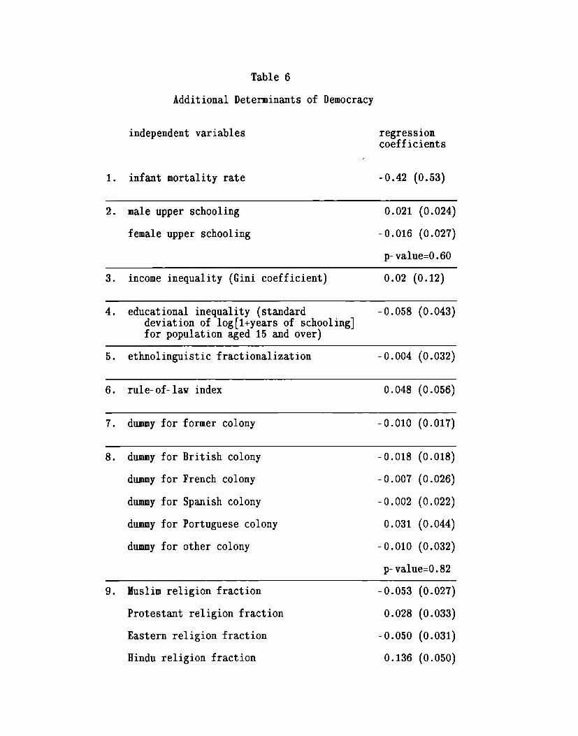
Table 6
Additional Determinmts of Democracy
independent variables regressioncoefficients
1. infant ❑ortality rate -0.42 (0.53)
2. male upper schooling 0.021 (0.024)
female upper schooling -0.016 (0.027)
p-value=O.60
3. income inequality (Gini coefficient) 0.02 (0.12)
4. educational inequality (standard -0.058 (0.043)deviation of log[l+years of schooling]for population aged 15 and over)
5. ethnolinguistic fractionalization -0.004 (0.032)
6. rule-of-law index 0.048 (0.056)
7. dummyfor former colony -0.010 (0.017)
8. dummyfor British colony -0.018 (0.018)
dummyfor French colony -0.007 (0.026)
dummyfor Spanish colony -0.002 (0.022)
dummyfor Portuguese colony 0.031 (0.044)
dummyfor other colony -0.010 (0.032)
p-value=O.82
9. Muslim religion fraction -0.053 (0.027)
Protestant religion fraction 0.028 (0.033)
Eastern religion fraction -0.050 (0.031)
Hindu religion fraction 0.136 (0.050)

Table 6, continued
independent variables regressioncoefficients
Jewish religion fraction 0.066 (0.079)
Creek Orthodox religion fraction 0.089 (0.053)
other or no religion fraction -0.030 (0.043)
p-value=O.005(without Hindu = 0.101)
Notes: The indicated groups of explanatory variables are added, one at atime, to the system for the democracy index shown in column 1 of Table 5.
ACase 6 applies only to the three periods that start uith the value of theemocracy index for 1985.) The infant mortality rate applies to 1965, 1970,
etc. Upper schooling is the years of secondary and higher schooling formales or females aged 15 and over in 1965, 1970, etc. Income inequality isthe Gini coefficient for income data applying around 1960 in the first threeequations and in the early 1980s in the last three equations. A highernumber indicates more inequality. Educational inequality is the standarddeviation of log(l+years of schooling) for the overall population aged 15 andover in 1965, 1970, etc. The ethnolinguistic fractionalization variable,which runs between O and 1, is a measure of heterogeneity of language andethnicity. The number, observed once for each country, represents theprobability that two randomly selected persons uill come from different
froups; hence, a higher value signifies more heterogeneity. See Mauro (1995)or a discussion of these data. The rule-of-law index, discussedby Knack
and Keefer (1995) and available for 1982-95 from Political Risk Services, isa subjective indicator of the extent of ❑aintenmce of the rule of law. Thevariable runs from O to 1, uith a higher value indicating a more favorableenvironment. Colony is a dummyfor countries that are former or presentcolonies, where my country that was independent before 1776 is designated asa non-colony. In case 8, dummies for former British, French, Spanish,Portuguese, and other colonies are added together to the system from column 1of Table 5. Colonial status is based on the most recent ruler; for exaple,the Philippines is attributed to the United States, rather than Spain. Incase 9, the fractions of the population affiliated with seven major religious
froups are entered together into the system from column 1 of Table 5. Theeft-out religion category is Catholic. The religion data, which are rough
estimates observed once per country in the late 1980s, are from CentralIntelligence Agency (1992). Eastern religions include Buddhist, Taoist,Confucian, and Shinto.
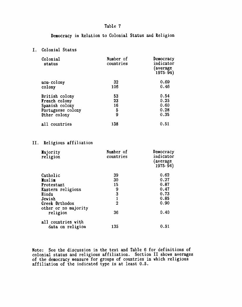
Table 7
Democracy in Relation to Colonial Status and Religion
I. Colonial Status
Colonialstatus
non-colonycolony
British colonyFrench colonySpauish colonyPortuguese colonyOther colony
all countries
II. Religious affiliation
Majorityreligion
CatholicMuslimProtestantEastern religionsHinduJewishCreek Orthodoxother or no majority
religion
all countries withdata on religion
Number ofcountries
32106
532316
59
138
Number ofcountries
36
135
Democracyindicator(average1975-94)
0.690.46
0.540.250.600.280.35
0.51
Democracyindicator(average1975-94)
0.620.270.870.470.730.850.90
0.40
0.51
Note: See the discussion in the text and Table 6 for definitions ofcolonial status and religious affiliation. Section II shows averagesof the democracy measure for groups of countries in which religiousaffiliation of the indicated type is at least 0.5.

Table 8
Actual and Long-Run Values of Democracy
Count ry
AlgeriaBeninBot sw~aCameroonCent. Afr. Rep.
CongoEgyptC-biaGhanaGuinea- Bissau
KenyaLesothoLiberiaMalawiMali
Haurit iusMozambiqueNigerRwandaSenegal
Sierra LeoneSouth AfricaSudanSwazilandTazaia
TogoTunisiaUgandaZaireZambia
ZimbabueBarbadosCanadaCosta Rica
Democ. 75actual
0.170.000.830.170.00
0.330.170.830.000.17
0.330.330.170.000.00
0.830.170.000.000.17
0.170.500.170.170.17
0.000.170.000.000.33
0.171.001.001.00
Dominican Republic 0.50
El Salvador 0.83Guatemala 0.50Haiti 0.17Honduras 0.17Jamaica 1.00
Democ. 75projected
0.010.360.510.270.15
0:38*0.18*0.25-.
0.230.590.250.060.17
0.480.330.270.310.22
0.180.640.330.450.21
0.210.350.270.150.15
0.410.840.960.760.57
0.460.500.360.490.78
Democ. 75gap
0.16-0.36
0.32-0.10-0.15
-0;210.65
-0.25--
0.10-0.25-0.08-0.06-0.17
0.35-0.16-0.27-0.31-0.05
-0.01-0.14-0.16-0.29-0.05
-0.21-0.19-0.27-0.15
0.18
-0.240.160.040.24
-0.07
0.370.00
-0.19-0.32
0.22
Democ. 94actual
0.000.830.830.170.67
0.500.170.000.330.67
0.170.500.000.830.83
1.000.670.670.000.50
0.000.830.000.170.17
0.170.170.330.000.67
0.331.001.001.000.50
0.670.500.330.670.83
Democ. 94projected
0.200.240.760.380.13
0.480.440.170.210.18
0.380.76
0:210.27
0.750.320.320.300.28
0.160.610.390.540.26
0.150.360.320.070.07
0.480.92
(1.06)0.860.66
0.630.630.210.450.81
Democ. 94gap
-0.200.590.08
-0.210.54
0.02-0.27-0.17
0.120.48
-0.21-0.26
0:630.56
0.250.340.34
-0.300.22
-0.160.23
-0.39-0.37-0.10
0.01-0.19
0.02-0.07
0.60
-0.140.08
-0.060.14
-0.16
0.03-0.130.130.220.03

Table 8, continued
Country
MexicoNicaraguaPanamaTrinidad & Tob.United States
Ar entinafBo ivia
BrazilChileColombia
EcuadorGuyanaParaguayPeruUruguay
VenezuelaBahrainBangladeshChinaHong ~Ong
IndiaIndonesiaIranIraqIsrael
JapanJordanSouth KoreaMalaysiaNepal
PakistanPhilippinesSingaporeSri LankaSyria
TaiwanThailandAustriaBelgiumCyprus
Democ. 75actual
0.500.330.000.831.00
0.500.170.500.000.83
0.000.500.330.170.33
0.830.170.000.000.67
0.830.330.170.000.83
0.830.170.330.670.17
0.330.330.330.830.17
0.170.831.001.000.50
Democ. 75projected
0.560.530.740.85
(1.02)
0.740.250.640.650.59
0.590.670.610.410.75
0.53--
0.380.53*0.45
0.20(-0.05)
0.220.150.71
0.910.220.500.400.34
0.300.620.360.700.29
0.550.550.890.930.67
Democ. 75gap
-0.06-0.19-0.74-0.02-0.02
-0.24-0.09-0.14-0.650.25
-0.59-0.17-0.27-0.25-0.41
0.30
-0:38-0.530.22
0.630.38
-0.05-0.150.12
-0.08-0.06-0.17
0.27-0.17
0.03-0.29-0.030.13
-0.13
-0.380.280.110.07
-0.17
Democ. 94actual
0.500.500.831.001.00
0.830.830.830.830.67
0.830.830.500.330.83
0.670.170.830.000.33
0.500.000.170.001.00
0.830.500.830.500.67
0.670.670.330.500.00
0.670.671.001.001.00
Democ. 94projected
0.800.560.790.88
(1.11)
0.760.450.760.740.83
0.720.650.680.550.77
0.460.430.460.530.85
0.380.250.260.090.86
(1.06)0.570.810.730.33
0.440.740.730.820.54
0.860.871.00
(1.01)0.93
Democ. 94gap
-0.30-0.060.040.12
-0.11
0.070.390.080.09
-0.16
0.110.19
-0.18-0.210.07
0.21-0.27
0.37-0.53-0.51
0.12-0.25-0.10-0.09
0.14
-0.23-0.07
0.03-0.23
0.34
0.23-0.07-0.39-0.32-0.54
-0.19-0.20
0.00-0.01
0.07

Table 8, continued
Country
DenmarkFinlandFranceWest GermanyGreece
HaryYIce and
IrelandItalyNetherlands
NorwayPolandPortugalSpainSweden
SwitzerlandTurkeyUnited KingdomYugoslaviaAustralia
FijiNew ZealandPapua New Guinea
Democ. 75actual
1.000.831.001.000.83
0.171.001.001.001.00
1.000.170.330.330.83
1.000.671.000.171.00
0.831.000.67
Democ. 75projected
0.90(1.04)0.920.970.65
0.940.800.900.880.92
0.990.800.730.820.90
(1.02)0.460.940.650.92
0.520.890.46
Democ. 75gap
0.10-0.20
0.080.030.18
-0.770.200.100.120.08
0.01-0.63-0.40-0.49-0.07
-0.020.210.06
-0.480.08
0.310.110.21
Democ. 94actual
1.001.001.001.001.00
1.001.001.001.001.00
1.000.831.001.001.00
1.000.331.000.171.00
0.501.000.83
Democ. 94projected
0.96
11
1.081.011.050.71
0.830.891.000.960.97
1.000.860.950.990.98
(1.06)0.72
(1.02)0.701.00
0.750.950.50
Democ. 94gap
0.04-0.08-0.01-0.05
0.29
0.170.110.000.040.03
0.00-0.030.050.010.02
-0.06-0.38-0.02-0.53
0.00
-0.250.050.33
Note: Projected values are based on the estimated system shown in Table 5,column 1. The 1975 projection is [1/(1-coeff. of lagged democracy)]*(estimated value based on other variables included in the 1975 equation).The 1994 projection is formed analogously. Values in parentheses arelinearly fitted values that lie outside the range (0,1). Values shown inbold have a magnitude of at least 0.33.
*Long-run projected value based on variables included in the 1980 equation.

Variable
1960-70:inflation rate
standard deviationof inflation rate
1970-80:inflation rate
standard deviationof inflation rate
1980-90:inflation rate
standard deviationof inflation rate
Table 9
Descriptive Statistics on Inflation
Hem Median Number of Countries
.054 .033 117
.039 .024 117
.133
.075
.191
.134
.101
.054
.089
.049
122
122
119
119
Notes: The inflation rate is computed on an annual basis for each countryfrom data on consumer price indexes (from the World Bd, STARSdatabank andissues of Yorld Tables; International Monetary Fund, Internuiionul Financial$tatistics, yearbook issues; and individual country sources). In a fewcases, figures on the GDPdeflator were used. The average inflation rate foreach country in each decade is the mean of the annual rates. The standarddeviation for each country in each decade is the square root of the averagesquared difference of the annual inflation rate from the decadal mean. Thevalues shown for inflation in this table are the mean or median across thecountries of the decade-average inflation rates. Similarly, the figures forstandard deviations are the mem or median across the countries of thestandard deviations for each decade.
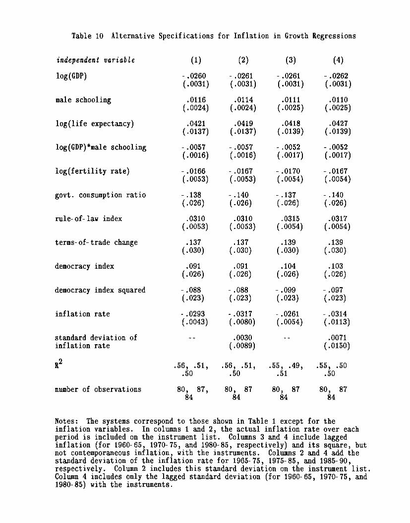
Table 10 Alternative Specifications for Inflation in Grouth Regressions
independent variable
log(GDP)
male schooling
log(life expectmcy)
log(GDP)*male schooling
log(fertility rate)
govt. consumption ratio
rule-of-law index
terms-of-trade change
democracy index
democracy index squared
inflation rate
standard deviation ofinflation rate
R2
number of observations
(1)
-.0260(.0031)
.0116( .0024)
.0421(.0137)
-.0057(.0016)
-.0166(.0053)
-.138(.026)
.0310(.0053)
.137(.030)
.091(.026)
-.088(.023)
-.0293(.0043)
--
.56, .51,.50
80, 87,84
(2)
-.0261(.0031)
.0114( .0024)
.0419(.0137)
-.0057(.0016)
-.0167(. 0053)
-.140(.026)
.0310(.0053)
.137(.030)
.091(.026)
-.088(.023)
-.0317( .0080)
.0030(.0089)
.56, .51,.50
80, 8784
(3)
-.0261(.0031)
.0111(.0025)
.0418(.0139)
-.0052(.0017)
-.0170(.0054)
-.137(.026)
.0315(.0054)
.139(.030)
.104(.026)
-.099(.023)
-.0261(.0054)
--
.55, .49,.51
80, 8784
(4)
-.0262(.0031)
.0110(.0025)
.0427(.0139)
-.0052(.0017)
-.0167(.0054)
-.140(.026)
.0317(. 0054)
.139(.030)
.103(.026)
-.097(.023)
-.0314(.0113)
.0071(.0150)
.55, .50.50
80, 8784
Notes: The systems correspond to those shown in Table 1 except for theinflation variables. In columns 1 and 2, the actual inflation rate over eachperiod is included on the instrument list. Columns 3 and 4 include laggedinflation (for 1960-65, 1970-75, and 1980-85, respectively) and its square, butnot contemporaneous inflation, with the instruments. Columns 2 and 4 add thestandard deviation of the inflation rate for 1965-75, 1975-85, and 1985-90,respectively. Column 2 includes this stadard deviation on the instrument list.Column4 includes only the lagged stadard deviation (for 1960-65, 1970-75, and1980-85) with the instruments.

Table 11
High-Inflation Observations
(values for which the period-average inflation rate exceeds 40Z per year)
Count ry
1965-75:
ChileIndonesiaUruguay
1975-85:
Ar entinafBo ivia
BrazilHaitiIsrael
PeruUgandaUruguayZaire
1985-90:
ArgentinaBrazilGuinea-Bissau*HexicoMozambique*
NicaraguaPeruPoland*Sierra LeoneTurkey
UgandaUruguayYugoslaviaZaireZambia
Inflation rate
0.680.530.50
1.261.060.660.480.78
0.560.530.410.44
1.922.040.530.530.48
1.872.220.810.630.43
0.780.581.410.590.56
*Not included in regression sample because of missing data on other variables.

Table 12
Inflation Rates and Central Bti Independence
Country
West GermanySwitzerlandAustriaEgyptDenmark
Costa RicaGreeceUnited StatesEthiopiaIreland
PhilippinesBahamasTanzaniaNicaraguaIsrael
NetherlandsCanadaVenezuelaBarbadosArgentina
EondurasPeruChileTurkeyMalta
IcelmdKenyaLuxembourgZaireHexico
IndonesiaBotswanaGhanaFranceZambia
Index ofbank
indep.
0.710.650.650.570.53
0.520.520.510.500.50
0.490.480.480.470.47
0.470.470.450.440.44
0.440.440.430.420.42
0.420.400.400.390.37
0.360.360.350.340.34
Inflationrat e,
1960-90
0.0370.0380.0430.0940.069
0.1170.1090.0490.0580.083
0.1070. 063*0.1330.4360.350
0.0450.0540.1000.0750.891
0.0580.6060.4160.2350.035
0.2290.0820.0440.3570.227
0.3660.0760.2560.0640.174
Country
South AfricaNi eria
!Ma aysiaUgadaItaly
FinlandSwedenSingaporeIndiaUnited Kingdom
South KoreaChinaBoliviaUruguayBrazil
AustraliaThailandWestern SamoaNew ZealandNepal
PanmaZimbabweHungaryJapanPakistan
ColombiaSpainMoroccoBelgiumYugoslavia
PolandNorway
Index ofbank
indep.
0.330.330.320.320.31
0.300.300.300.300.30
0.290.290.290.290.28
0.270.270.260.250.23
0.230.220.210.200.19
0.190.160.150.130.12
0.120.12
Inflationrat e,
1960-90
0.0990.1250.0340.3530.088
0.0730.0670.0340.0740.077
0.1130.0390.4660.4410.723
0.0670.0520.112**0.0850.084
0.0330.0740.0470.0540.072
0.1700.0960.0550.0480.395
0.293*0.066
*1970-90**1975-90

Notes to Table 12: The index of central bank independence is computed from datain Cukierman (1992, Chapter 19, Appendix A). The index is a weighted average ofthe available data from 1950 to 1989 of legal provisions regarding1. appointment and dismissal of the governor (wei ht 1/6), 2. procedures for the
fformulation of monetary policy (weight 1/6), 3. 0 jectives of central bti
$!policy wei ht 1/6), and 4. limitations on lending by the central bank (weight
i12). he irst category is an unwei hted average of three underlying variables
ft at involve the governor’s term of o fice and the procedures for appointmentand dismissal. The second category is an unweighed average of two variables,one indicating the location of the authority for setting monetary policy and theother specifying methods for resolving conflicts about policy. The thirdcategory relates to the prominence attached to price stability in the bank’scharter. The fourth cate ory is an unweighed avera e of four variables:limitations on advances, f !imitations on securitized ending, an indicator forthe location of the authority that prescribes lending terms, and the circle ofpotential borrowers from the central bank. For each underlying variable,Cukierman defines a scale from O to 1, where O indicates least favorable tocentral bank independence and 1 indicates most favorable. The overall indexshown in Table 12 runs correspondingly from O to 1. See Table 8 for adiscussion of the inflation data.

Period
1960-70
1970-80
1980-90
1960-90
Table 13
Inflation Rates and Prior Colonial Status
All Non-Countries Colony
.054(121)
.131(131)
.182(132)
.126(117)
.045(31)
.110(32)
.124(31)
.089(30)
BritishColony
.033(43)
.120(50)
.139(51)
.104(42)
FrenchColony
.030(21)
.093(20)
.074(22)
.066(20)
Spanish Otheror Port. ColonyColony
.089 .194(19) (7)
.218 .147(21) (8)
.523 .136(20) (8)
.294 .161(18) (7)
addendum:Latin Amer.not Spanishor Port.Colony
.031(7)
.109(11)
.097(11)
.090(7)
Notes: The numbers shown in parentheses are the numbers of countries withavailable data that fall into each category. See Table 9 for a discussion ofthe inflation data. Countries that were independent before 1776 are treatedas non-colonies. Otherwise, the colonial status refers to the most recentoutside power; for exwple, the Philippines is attributed to the UnitedStates, rather than Spain; Rwanda and Burundi are attributed to Belgium,rather than Germany; md the Dominican Republic is attributed to France,rather than Spain. Some countries that were dominated by other countries forsome periods are treated as non-colonies; examples are Hungary, Poland, SouthKorea, and Taiwm. The only present colony in the sample is Hong Kong. Thelast column refers to countries that are located in Latin America but are notformer Spanish or Portuguese colonies.
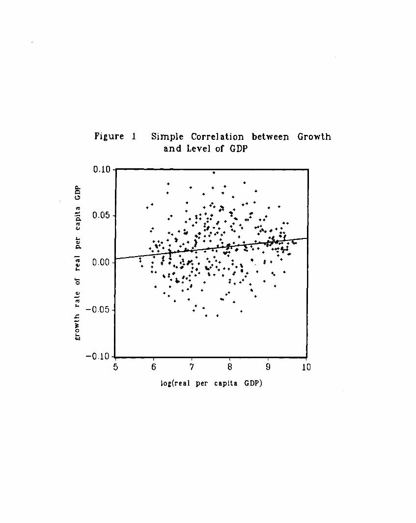
Figure 1 Simple Correlation between Growth
and Level of GDP
0.10
0.05
0.00
+ ++ ++
● ☞☞
☞☞
●☞
++ +++
+++ ●
☞☞
☞☞
●▼☞
$+:
++
+ ++ ● + +
●+ ●
+ + *+ ++
+++ +
++
5 6 7 8 9 10
log(real per capita GDP)

rlgure G tirowtn Hate versus Level 01. .
- GDP
0.15
0.10
0.05
0.00
–0.05
-0.105 6 7 8 9 10
log(real per capita GDP)

Figure 3 Growth Rate versus Male Schooling
0.10
0.05
0.00
-0.05
–0.10
+++ ●
●
●❆4
0123456 7
years of secondary & higher school, males 25 and older
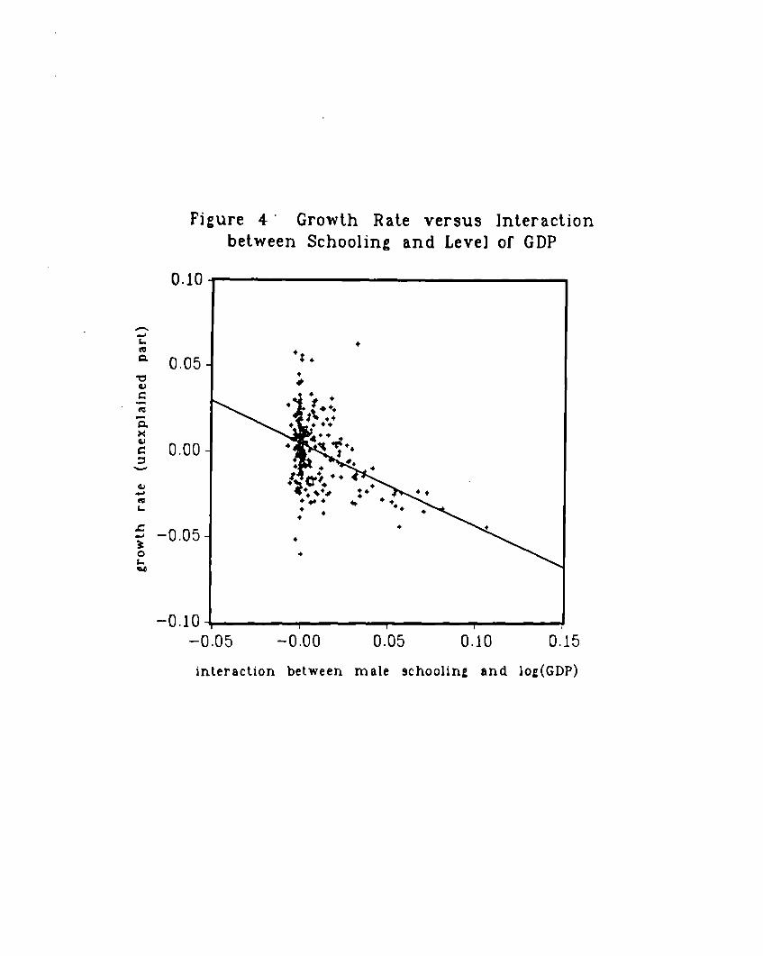
Figure 4 “ Growth Rate versus Interaction
between Schooling and Level of GDP
0.10
0!05
000
-0.05
-O.10–0.05 -0.00 0.05 0.10 0.15
interaction between male schooling and log(GDP)

n
Figure 5 Growth R ate versus Ljfe Expectancy
O.10
0.05
0.00
+
++
3,25 3.50 3.75 4100 4.25 450
log(life expectancy at birth)

-. — .Figure 6 Growth R ate versus Fertility Rate
0.10
0.05
0.00
–0.05
-0.10
++++ +
+ t+ +* ++++● ☞ ● 4
● +
++
+ ++
0.0 0.5 1.0 1.5 2.0 2.5
log(total fertility rate)

n
0.10
0105
0.00
Figure 7 Growth Rate versus
Government Consumption Ratio
+
+ +●
0.0 0.1 0.2 0.3 0.4 0.5
ratio of government consumption to CDP
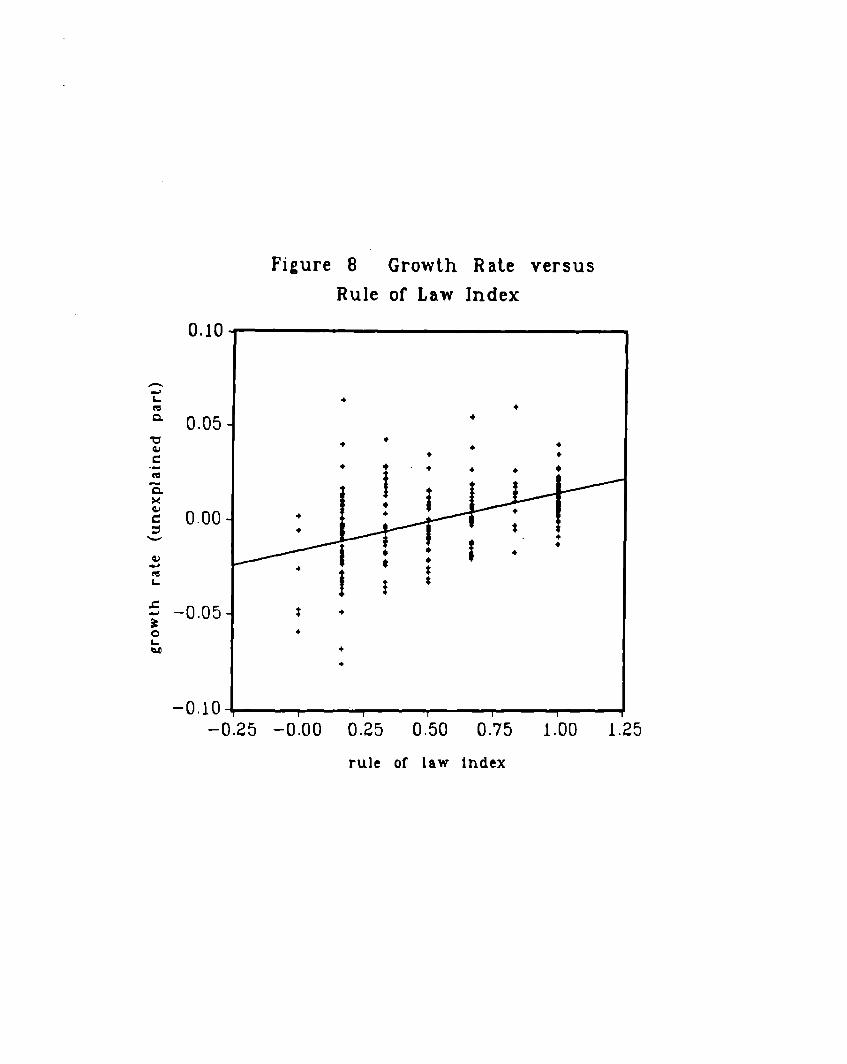
0.10
0.05
0.00
–0.05
–010
F]gure 8 Growth Rate versus
Rule of Law index
–0.25 –OiOO 0.25 0.50 0.75 1.00 1.25
rule of law index
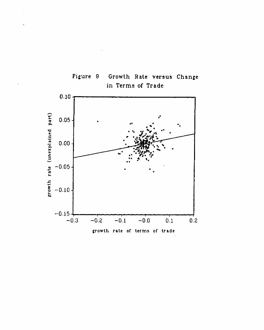
0.10
0.05
0.00
-0.05
-0.10
-0.15
Figure 9 Growth Rate versus Change
in Terms of Trade
–0.3 -0.2 –0.1 –Oho O.l 0.2
growth rate of terms of trade

0
?
. . . . . . . . . . ,. . . . . . . . . ...
. . . . . . .
. . . .
. .
. .
,...
..:.
. . . . .
,..
\II\
\
. . . . . .
., .,..
.,
\t\
\\.
1:\
. . . . . \, .:.,.
\:\
\.\
. . . . . . . . .
. . . .
:1\
“\,. ..,.. . . .. .t
#?\’
\:
/:/
/./.####/,* .,/,#/./#@.
H ‘;/.#.0
#
,..,.. ,..:,> F,’.,. . . . . . . . . . . . . . . . . . ... . . . . . . . . . . . . . .,4
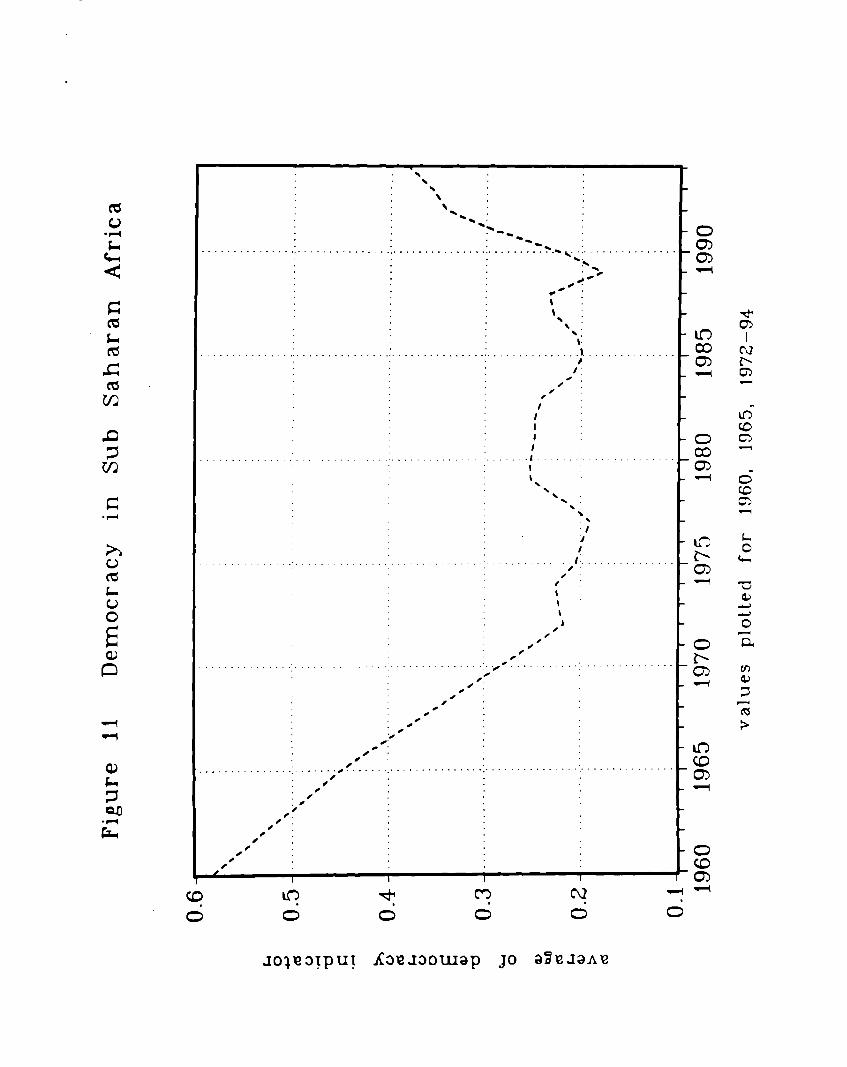
#
o
. . . . . . .,.-... . . . . . . .,. . .
\\
-U* ;-% -~
.-. . . . . . . ... . . . . . -.. .
t:\~:
● ✌
✼
✌✎ ✌✌✌ ✎✌ ✎ ✎✌ 1 . . . . . . . . . . . . . ./
I1 . . . .
“1
I
.,..,. . . . . . . . . . . 1 . . . . . . . . . . . ./
o

$.*VI
?0
N
0
. . . . s-< . . . . . . . . . . . . . . . . ... . . . .*N
-:.\
., ..., . . . . . . . . . . . ... . . . . . . . . . . . . . . . . . . . . . . .
#:/
#/:
/,0,
I I I I I
m
o o 0
o-
:

Figure13 Growth Rateversus indicator of Democracy
0.10
0.05
0.00
-0.05
-Omlo
+
+ ++
+++ +
++
++
-0.2 0.0 0.2 0.4 0.6 0.8 1.0 1.2
index of political rights

200
150
100
50
0
12.5
10.0
7.5
5.0
2.5
0.0
Figure 14 Histograms for Inflation Rate
0.00 0:30 0.’60 0.’90 1.20 1!’50
Inflation rate
0:35 0:70 1.05 1.40 1.75
itilttion rob (for values above 20% per Yem)

Figure 15 Standard Deviation of
inflation Versus Mean inflation
.
.. .,.. . .,
. .
mb 4k oh 0.’10 a
,,
0:0 ok 1:0 1:5

Figure 16 Growth Rate versus
Inflation Rate
OM . . . .,.. .
Om. ‘:
..

i
1.00
0.75
0.50
0.25
0.00
Figure 17 Inflation and
Central Bank Independence
+
+
0.1 0.2 0.3 0.4 0.5 0.6 0.7 0.8
index of central-bank independence, 1950–89
Top Related