


Languages
Pages
Legal

TRACE Deliverable 7.3
November 2007 - 1 -
Project No. 027763 – TRACE
Deliverable 7.3
Analysis Methods for Accident and Injury Risk Studies
Contractual Date of Delivery to the CEC: October 2007
Actual Date of Delivery to the CEC: November 2007
Authors: Heinz Hautzinger, Claus Pastor, Manfred Pfeiffer, Jochen Schmidt
Participants: IVT, BASt
Work package: 7
Est. person months: 8
Security: PU
Nature: Report
Version: 2
Validation by WP leader: Heinz Hautzinger
Validation by TRACE Coordinator: Yves Page
Reviewed by external reviewer: Prof. Dr. O. Schwarz (Heilbronn University of Applied Sciences)
Total number of pages: 72
Abstract:
In studies of traffic accident causation the researcher aims at the assessment of risk factors for accident involvement and accidental injury. Consequently, Task 7.3 “Analysis methods for accident and injury risk studies” provides the operational work packages of TRACE with appropriate methodological tools from accident and injury epidemiology. As different types of accident and exposure databases are encountered in the TRACE project, special emphasis is placed on study designs which fit to the available data sources. Taylor-made statistical tools as presented in this report enable accident researchers to identify whether there is a relationship between a set of potential risk factors and accident involvement or accidental injury. In order to make the statistical concepts and methods compiled under Task 7.3 easily accessible also to researchers which are not experts in statistics and/or epidemiology, numerous examples and detailed empirical case studies have been integrated in the report. Results from the work under Task 7.3 are described in detail in this report. An extended non-technical summary of the results will be provided in TRACE Deliverable 7.5 “WP7 Summary Report”.
Keyword list:
Traffic accidents, accident causation, involvement risk, injury risk, risk measures, risk factors, statistical methods, epidemiological methods, study designs, accident involvement surveys, cohort studies, case-control studies, induced exposure analyses
TRACE Deliverable 7.3
November 2007 - 2 -
Table of Contents
1 Executive Summary__________________________________________________________ 5
2 Introduction and Conceptual Framework _______________________________________ 7
2.1 Introduction ___________________________________________________________ 8
2.2 Traffic Participation and Accident Involvement ____________________________ 8
2.2.1 Basic conceptual considerations________________________________________________ 8
2.2.2 Traffic participation __________________________________________________________ 9
2.2.3 Traffic accident involvement _________________________________________________ 10
2.2.4 Multilevel structure of trip-making and accident involvement data ________________ 10
2.3 Population at Risk _____________________________________________________ 11
2.3.1 Trip level analysis___________________________________________________________ 11
2.3.2 Person-year level analysis ____________________________________________________ 12
2.3.3 Need for precise definition of the population at risk _____________________________ 13
2.4 Samples from the Population at Risk ____________________________________ 13
2.4.1 Sampling from a population of trips ___________________________________________ 13
2.4.2 Sampling from a population of person-years____________________________________ 14
2.4.3 Sampling from an unspecified population at risk ________________________________ 14
2.5 Risk Factors ___________________________________________________________ 15
2.5.1 Risk factors as attributes of the units at risk_____________________________________ 15
2.5.2 Measuring risk factors _______________________________________________________ 16
2.6 Investigating Traffic Accident Causation _________________________________ 16
2.6.1 Accident cause as a measurable characteristic of accidents and road users involved __ 16
2.6.2 Accident causes as proven risk factors for accident involvement ___________________ 18
2.6.3 Statistical analysis methods for accident causation studies ________________________ 18
3 Measures of Chance of Traffic Accident Involvement ____________________________ 20
3.1 Overview _____________________________________________________________ 20
3.2 Risk of Accident Involvement___________________________________________ 20
3.2.1 Risk_______________________________________________________________________ 20
3.2.2 Relative risk________________________________________________________________ 21
3.2.3 Attributable risk ____________________________________________________________ 22
3.3 Odds of Accident Involvement __________________________________________ 22
3.3.1 Odds______________________________________________________________________ 22
3.3.2 Odds ratio _________________________________________________________________ 22
3.4 Accident Involvement Rate _____________________________________________ 23
3.4.1 Rate_______________________________________________________________________ 23
3.4.2 Types of accident involvement rates ___________________________________________ 23
TRACE Deliverable 7.3
November 2007 - 3 -
3.4.3 Relative rate________________________________________________________________ 23
3.5 Accident Involvement Density __________________________________________ 23
3.5.1 Time-related accident involvement density _____________________________________ 24
3.5.2 Distance-related accident involvement density __________________________________ 24
3.5.3 Relative density ____________________________________________________________ 24
3.6 A Note on the Differences between Risks, Odds, Rates and Densities _______ 24
4 Statistical Models for Alternative Measures of Chance of Accident Involvement____ 26
4.1 Criteria for Choosing a Statistical Model for the Measure of Chance_________ 26
4.2 Models for Risk and Relative Risk_______________________________________ 26
4.2.1 A binomial model for traffic accident involvement risk___________________________ 26
4.2.2 A normal distribution model for the log of the relative risk _______________________ 27
4.2.3 A normal distribution model for the attributable risk ____________________________ 27
4.2.4 Logistic regression models for accident involvement risk _________________________ 28
4.3 Models for Odds and Odds Ratio________________________________________ 28
4.3.1 A normal distribution model for the log of the odds ratio_________________________ 28
4.3.2 Regression model for the log odds of accident involvement _______________________ 28
4.4 Models for Rates and Densities _________________________________________ 29
4.4.1 Poisson model for accident involvement counts _________________________________ 29
4.4.2 Poisson model for accident involvement rates and densities ______________________ 29
4.4.3 Log-linear models for accident involvement counts, rates and densities_____________ 30
5 Databases for Accident Involvement Risk Studies ______________________________ 31
5.1 Usage of Routine Data versus Special Data Collection _____________________ 31
5.2 Individual versus Grouped Data ________________________________________ 31
5.3 Sources of Data on Accident Involvement and Causation___________________ 31
5.4 Sources of Data on Exposure to Accident Involvement Risk ________________ 32
5.5 Combining Accident and Exposure Data from Different Sources____________ 32
6 Study Designs for Accident Involvement Risk Analyses _________________________ 33
6.1 Studies Based on Special Samples from the Population at Risk _____________ 33
6.1.1 One sample: Accident involvement incidence survey ____________________________ 33
6.1.2 One sample: Cohort study of traffic accident involvement ________________________ 34
6.1.3 Two independent samples: Case-control study of traffic accident involvement ______ 35
6.2 Studies Combining Accident and Exposure Data from Different Sources ____ 37
6.2.1 Accident counts related to counts of units at risk (involvement risk) _______________ 37
6.2.2 Accident counts related to trip length and trip time totals (involvement density)_____ 40
6.3 Studies Based Solely on Accident Data: The Concept of “Induced Exposure” _ 42
6.3.1 Idea behind the concept______________________________________________________ 42
6.3.2 Comparison of responsible and non-responsible drivers__________________________ 42
TRACE Deliverable 7.3
November 2007 - 4 -
6.3.3 Comparison of risk factor-specific and reference accident type ____________________ 45
6.4 Criteria for Choosing Among Alternative Study Designs___________________ 46
7 Measuring Road User Injury Risk ____________________________________________ 47
7.1 Unconditional Road User Injury Risk ____________________________________ 47
7.2 Conditional Road User Injury Risk ______________________________________ 48
8 Conclusions _______________________________________________________________ 49
References _____________________________________________________________________ 50
Annex I ________________________________________________________________________ 52
Accident Involvement and Injury Risk Analyses Combining Data from Different Sources _____________________________________________________________________ 52
Part A: Distance- Related Accident Involvement Density δDistance __________________ 52
Part B: Time-Related Accident Involvement Density δTime ________________________ 55
Part C: Unconditional Road User Injury Risk ρTrip _______________________________ 58
Annex II _______________________________________________________________________ 62
Study Designs Based on Sampling from the Population at Risk ___________________ 62
Part A: Survey on Accident Involvement and Injury Incidence ____________________ 62
1. Description of the Survey_______________________________________________________ 62
2. Sample measures of chance of accident involvement _______________________________ 62
3. Involvement risk estimation for an actual finite population at risk____________________ 62
4. Involvement risk estimation for a hypothetical population at risk ____________________ 63
5. Differentiating between several types of accident involvement ______________________ 63
6. Conditional risk of injury given accident involvement ______________________________ 64
Part B: Case-Control Study of Accident Involvement _____________________________ 65
1. Description of the data sets used ________________________________________________ 65
2. Assessing a dichotomous risk factor _____________________________________________ 65
3. Assessing a polytomous risk factor ______________________________________________ 66
4. Assessing several risk factors simultaneously _____________________________________ 67
Annex III ______________________________________________________________________ 71
The Concept of Induced Exposure: An External Validity Check____________________ 71
1. Problem formulation and methodological approach________________________________ 71
2. Nonresponsible car drivers compared to all car driver trips on the road_______________ 71
3. Bias of risk estimates obtained from induced exposure analyses _____________________ 72
TRACE Deliverable 7.3
November 2007 - 5 -
1 Executive Summary
General Overview
The TRACE project deals with traffic accident causation. In order to support the research on the causes of traffic accidents in Europe, analysis methods for accident involvement and injury risk studies have been investigated and compiled under Task 3 of Work Package 7 for use in the various operational work packages of TRACE.
According to the different types of accident and exposure data bases available in TRACE, the task was subdivided into three sub-tasks:
- Subtask 7.3.1: Studies based on aggregate accident and exposure data from different sources
- Subtask 7.3.2: Studies using solely accident data: the concept of “induced exposure”
- Subtask 7.3.3: Accident involvement surveys, cohort and case-control studies
The three subtasks of Task 7.3 are very closely related as they correspond to different study designs for empirical investigations on accident involvement and injury risk. Consequently, instead of three different subtask reports a single comprehensive report on Task 7.3 has been prepared.
Overview of Concepts and Methods
As accident involvement is an event occurring in time and space, the general epidemiological concept of disease incidence (incidence = number of new cases of a disease within a specified period of time) applies to studies on accident involvement risk. In the report, an overview of statistical methods is presented which prove to be especially suitable for investigations on the risk of accident involvement, accident causation and accidental injury.
Different descriptive measures of chance of accident involvement and accidental injury are considered in the report:
• Risk, relative risk and attributable risk • Odds and odds ratio • Incidence rate and incidence rate ratio (relative rate)
o per-capita accident involvement rate o per-vehicle accident involvement rate
• Incidence density and incidence density ratio (relative density) o trip distance-related accident involvement density o trip time-related accident involvement density
For the various risk measures appropriate statistical models have been investigated enabling the researcher to identify and assess risk factors and accident causes:
• Models for risk, relative risk and attributable risk o binomial model for accident involvement risk o normal distribution model for the log of the relative risk o model for the attributable risk o logistic regression model for involvement risk
• Models for odds and odds ratio o normal distribution model for the log of the odds ratio o regression model for the log odds of accident involvement
• Models for rates and densities o Poisson model for accident involvement counts o Poisson model for accident involvement rates and densities o Log-linear models for counts, rates and densities
TRACE Deliverable 7.3
November 2007 - 6 -
The above risk measures and models are also suitable to assess the risk of being injured in a road traffic accident. Here, a distinction has been made between the unconditional injury risk associated with traffic participation and the road user’s risk to receive an injury given that he or she is involved in an accident (conditional injury risk).
A new conceptual framework for accident involvement and injury risk studies is proposed in the report tying together methodological concepts of mobility behaviour analysis and traffic safety research. The idea behind this concept is that “accident involvement” is just another word for “accidental trip”: Whenever a trip (person or vehicle trip) terminates premature and unplanned due to involvement in a traffic accident, the corresponding trip may be classified as “accidental”. From a mobility research point of view, therefore, accident involvement can simply be regarded as another dichotomous trip characteristic (accidental trip yes/no).
Under this micro perspective, the universe of all trips on the road system is the natural “population at risk” of a study of accident involvement. This approach offers the possibility to develop a clear and unified epidemiological framework for the investigation of accident involvement and injury risk at different levels of aggregation (e.g. trip level or person-year level).
The following study designs are considered in the report:
• studies based on grouped (routine) accident and exposure data from different sources • studies based on special samples from the population at risk
o accident involvement surveys o cohort studies of accident involvement o case-control studies of accident involvement
• studies based solely on accident data: the concept of “induced exposure”
It appears that due to the variety of databases available, all these study designs are suitable for application in the TRACE project.
Numerical Examples and Empirical Case Studies
In order to make the concepts and methods compiled under Task 3 easily accessible also to researchers which are not experts in statistics and/or epidemiology, numerous examples and empirical case studies have been integrated in the report.
Non-technical Summary of Results
Results of the work completed under Task 7.3 are described in detail in this report. An extended non-technical summary of the results will be provided in TRACE Deliverable 7.5 “WP7 Summary Report”.
TRACE Deliverable 7.3
November 2007 - 7 -
2 Introduction and Conceptual Framework
The development of intelligent transport systems in vehicles or on roads (and especially in the safety field) must be preceded and accompanied by a scientific accident analysis encompassing two main issues:
• The identification and the assessment among the possible technology-based safety functions of the most promising solutions (in terms of lives saved and accidents avoided) that can assist the driver or any other road users in a normal road situation or in an emergency situation or, as a last resort, mitigate the violence of crashes and protect vehicle occupants, pedestrians, and two-wheelers in the case of a crash or rollover.
• The determination and the continuous up-dating of the aetiology, (i.e. the causes of road accidents and injuries) and the assessment of whether the existing technologies or those under development actually address road users' real needs, as inferred from accident and driver behaviour analyses.
These two main orientations of TRACE can be subdivided into several scientific objectives:
The definition of accident causation: Many factors influence a country’s transportation safety level. These factors concern road safety policy, distribution and crashworthiness of the fleet, road network characteristics, human behaviour and attitudes, travel conditions, environment, etc. These issues have been studied for decades and considerable prevention efforts have been inferred from the analysis and comprehension of these factors. Nevertheless, further efforts are needed. These factors have to be studied together in order to provide a comprehensive and understandable definition of accident causation.
Moreover, it is intended to provide the scientific community, stakeholders, suppliers, the vehicle industry and the other Integrated Safety program participants with a global overview of the road accident causation issues in Europe, based on the analysis of currently available databases which include accident, injury, insurance, medical and exposure data (including driver behavior in normal driving conditions). The aim is to identify, characterise and quantify the nature of risk factors, groups at risk, specific safety-related or risk-related societal issues, specific conflict driving situations and accident situations.
Another objective is to improve the multidisciplinary methodologies that are considered necessary to achieve this knowledge and especially methodologies for analysing the influence of human factors as well as the statistical methodologies used in risk and evaluation analysis.
This objective is addressed by the constitution of specific Work Packages devoted to methodologies which
• provide the operational Work Packages with tools and instruments for accident causation analysis and the assessment of the safety benefits of technologies
• identify and improve the scientific approaches in human factors analysis and statistical analysis applied to accident causation and evaluation
One of these specific Work Packages is WP 7 (“Statistical Methods”). Its main objectives are to improve statistical methodology in empirical traffic accident research (Tasks 7.1 to 7.4) and to provide statistical services and methodological advice to other work packages (Task 7.5). In particular the research activities under WP 7 are addressing the following subjects:
7.1 Methods for improving the usability of existing accident databases
7.2 Analysis methods for accident causation studies
7.3 Analysis methods for accident and injury risk studies
7.4 Methods for safety functions effectiveness evaluation and prediction
TRACE Deliverable 7.3
November 2007 - 8 -
2.1 Introduction
The focus of the TRACE project is on traffic accident causation. As always in empirical research, one can think of different ways to investigate traffic accident causation. Among the candidate methodologies the following two concepts are of special relevance:
• Case-by-case approach: Accident causes attributed to registered accidents and road users involved by expert judgement
• Statistical approach: Accident causes as risk factors for accident involvement
Basically, the case-by-case approach corresponds to direct measurement or rating of the cause or the causes of an individual accident. Thus, in a sense the process of attributing specific causes to registered accidents may be regarded as part of the data collection or data preparation phase. In contrast to this, the identification of accident causes, i.e. determinants of accident involvement, under the statistical approach is clearly part of the analysis phase1 of an accident causation study.
Since the TRACE project exclusively relies on existing European traffic accident and exposure databases, the statistical approach is primarily used in the operational work packages WP1 to WP4. However, as in many accident databases the person recording the accident (police officer or research team member) has described the causes of the accident in the corresponding survey form according to a given list of possible causes, traffic accident causation research in TRACE is also making use of data that have been generated under the case-by-case approach.
Task 3 of TRACE WP7 “Statistical Methods” is dealing with analysis methods for accident and injury risk studies. As accident determinants or accident causes are factors that precipitate accident occurrence, the concept of accident involvement risk suggests itself as a methodological framework for empirical accident causation studies. According to epidemiological principles, the determinants of accident involvement - also termed risk factors for accident involvement - are regarded as “accident causes” provided that the corresponding factors are sufficiently strong correlated with accident involvement and there is an appropriate theoretical explanation (aetiology of the accident). Fortunately, it appears that quite a number of the statistical methods of risk analysis can also be applied in studies based on data where accident cause is an “observed” variable according to the case-by-case approach.
In order to support the TRACE research activities on the causes of traffic accidents in Europe, analysis methods for accident involvement and injury risk studies have been investigated and compiled under Task 3 of WP 7 for use in the various operational work packages of TRACE. According to the different types of accident and exposure data bases available, work under Task 7.3 was subdivided into three sub-tasks:
• Subtask 7.3.1: Studies based on aggregate accident and exposure data from different sources
• Subtask 7.3.2: Studies using solely accident data: the concept of “induced exposure”
• Subtask 7.3.3: Accident involvement surveys, cohort and case-control studies
The three subtasks of Task 7.3 are, of course, very closely related as they correspond to different study designs for empirical investigations on accident involvement and injury risk. Consequently, instead of three different subtask reports a single comprehensive report on Task 7.3 has been prepared.
2.2 Traffic Participation and Accident Involvement
2.2.1 Basic conceptual considerations
From a public health point of view, incidence of accidental injury is a high-priority subject. Basically, for a given study period the observed number of cases of accidental injury depends on the following three quantities:
• number of units at risk (e.g. all drivers present on the road during the study period)
• risk of being involved in an accident when participating in traffic and
1 Data analysis is, of course, closely related to study design.
TRACE Deliverable 7.3
November 2007 - 9 -
• risk of being injured or killed when involved in a traffic accident.
Both types of risk mentioned above are of fundamental importance in traffic safety research. But as, by definition, accidental injury may only occur in accidents, accident involvement is perhaps the most basic phenomenon to be investigated in an empirical traffic safety study.
As accident involvement is an event occurring in time and space, the general epidemiological concept of disease “incidence” (incidence = number of new cases of a disease within a specified period of time) applies to studies on accident involvement risk. In this report an overview of statistical methods for epidemiological incidence studies is presented which appear to be useful for investigations on traffic accident involvement risk. To our knowledge, not all of these candidate methods have actually been applied in traffic safety research so far. The report draws on the following outstanding monograph as the basic epidemiological reference: Woodward, M.: Epidemiology – Study design and data analysis. Chapman & Hall/CRC, Boca Raton/London, 1999
In the following sections, a new conceptual framework for accident involvement risk studies is proposed where various methodological concepts are tied together that have been developed independently of each other in traffic safety research and mobility behaviour science.
The idea behind this innovative approach is that “accident involvement” is just another word for “accidental trip”: Person or vehicle trips terminating suddenly and unexpectedly due to involvement in a traffic accident may be classified as “accidental”, whereas all other trips may be termed “non-accidental”. Thus, from mobility behaviour research point of view accident involvement can be regarded as a dichotomous trip characteristic named “accident involvement status of trip”. Obviously, as in principle each trip may end up in an accident, trips are the basic units at risk and the characteristic “accident involvement status of trip” corresponds to “disease status of unit at risk” which is the usual criterion variable in epidemiological studies.
The above concept opens the possibility to develop a clear and unified framework for investigating traffic accident involvement and injury risk at different levels of aggregation using well-established epidemiological methods.
2.2.2 Traffic participation
By definition, road traffic accident involvement is an event which may only occur during participation in road traffic. Traffic participation or, equivalently, road use has a wide variety of forms of appearance. Basically, however, traffic participation is simply a spatio-temporal activity of a human being carried out with or without the aid of a (motorised or non-motorised) vehicle.
Subsequently, the acting person is called road user if he or she participates in road traffic as vehicle driver, vehicle rider or pedestrian. Although individuals who participate in road traffic as vehicle passengers also use the road system, they are not termed road users. Rather, vehicle passengers are said to be associated with a road user. Vehicle drivers/riders together with their associated vehicle passengers are termed vehicle users. Finally, vehicle users together with pedestrians will be called mobile persons. Thus, a mobile person is an individual who participates in road traffic within a specified period of time irrespective of travel mode.
Mobile persons may participate in traffic several times within a specified period. Every time a person appears in the road system, an additional traffic participation activity is generated. Consecutive traffic participation activities of the same mobile person may, of course, be made by different modes. For instance, after a short recreational walk around the block (traffic participation as a pedestrian) the person may drive to a supermarket for shopping (traffic participation as a car driver). In order to simplify the wording one may speak of a person-trip when a single traffic participation activity of a mobile person is to be addressed. According to this, mobile persons may also be called trip makers. In cases where the trip maker is a vehicle user, his or her person-trip is assigned to a vehicle-trip. The person-trips of vehicle users which are assigned to the same vehicle-trip form a trip cluster.
The universe of all trips generated by the members of a certain population of trip makers during a specific study period is of fundamental importance for any accident involvement study as this universe forms the “population at risk” in the epidemiological sense. A single element of the
TRACE Deliverable 7.3
November 2007 - 10 -
population at risk is called “unit at risk”. In our context trips are the units at risk. This wording simply expresses the fact that virtually any trip may end up in an accident. See Section 2.3 or details.
2.2.3 Traffic accident involvement
Road users who themselves or whose vehicle have suffered or caused damages are said to be involved in a traffic accident. Thus, traffic accident involvement is a situational characteristic of road users. More specifically, traffic accident involvement is a binary characteristic of road user trips in the sense that non-accidental and accidental road user trips can be distinguished.
Accident involvement status2 of the units at risk is the criterion variable in many traffic safety studies. Normally, accident involvement status will be measured at two levels (“accidental” and “non-accidental” trips). Sometimes, however, it may be necessary to distinguish different types of accident involvement. At the trip level, an example would be “at-fault” and “not at-fault” accident involvement, respectively. In this case, accident involvement status is a categorical trip attribute with three possible outcomes: at-fault accidental trip, not at-fault accidental trip and non-accidental trip3.
When a road user is involved in an accident, his or her vehicle (if any) and similarly the passengers of the vehicle he or she rides/drives may also be considered as accident-involved. A clear distinction, however, must be made between accident involvement of road users and accident involvement of mobile persons (pedestrians, vehicle riders/drivers, vehicle passengers).
Of course, two or more accident-involved road users may be involved in the same accident. In this case, an accident corresponds to a pair, triple etc. of accidental road user trips and one may speak of multiple road user accidents in contrast to single road user accidents (e.g. crash of a single car against a roadside tree). Any single road user accident is identical with an accidental road user trip.
2.2.4 Multilevel structure of trip-making and accident involvement data
Empirical data on traffic participation (trip-making) are collected in mobility surveys which normally make use of the trip or activity diary technique, respectively. Typically, all trips made by a selected person on a specific “travel day” - the day about which trip reporting should occur - are to be recorded. Thus, traffic participation data from mobility surveys usually have the following hierarchical structure:
Level 1: person
Level 2: day (person-day)
Level 3: trip
Typical trip characteristics recorded in mobility surveys are trip length and duration, trip purpose and trip mode.
If, in addition to the above mentioned trip characteristics, the attribute “accidental trip yes/no” would be recorded, one could call such a data acquisition system a combined trip-making and accident involvement survey. Surveys of this type would be ideal for accident involvement risk assessment. To our knowledge, however, no such survey at the trip level has ever been conducted in practice (due to the fact that accident involvement is a rare event, the sample size of such a survey had to be very large).
At a more aggregate level, however, specifically designed combined trip-making and accident involvement surveys may well be realistic. Consider, for instance, a survey where households are randomly selected from the population and all members of the chosen households are reporting for the last 12 months both their annual sum of car kilometres (km per year) and their number of accident involvements as car driver (0, 1, 2, …). Under such a design we would have the following two-level data structure:
2 Accident involvement status corresponds to the general term disease status used in epidemiology. 3 A two-car crash, for instance, corresponds to a pair of accidental car trips. Either accidental trip may be an at-
fault and not at-fault trip, respectively.
TRACE Deliverable 7.3
November 2007 - 11 -
Level 1: household
Level 2: person-year
The individual’s annual number of kilometres travelled by car and his or her annual number of accident involvements are characteristics of the study unit person-year.
Data solely on accident involved units are collected in traffic accident surveys which may be either a nation-wide census (police-recorded data) or a regional sample survey (in-depth data). Normally, such data will be analysed at the following three levels:
Level 1: accident
Level 2: road user involved
Level 3: vehicle passenger
The above considerations on the hierarchical or cluster structure of traffic participation and accident involvement data suggest that accident involvement risk may be investigated at different levels. The proper choice of the analysis level depends both on study purpose and data availability. In the sequel, two different levels of analysis, the trip level and the person-year level are considered in more detail.
2.3 Population at Risk
2.3.1 Trip level analysis
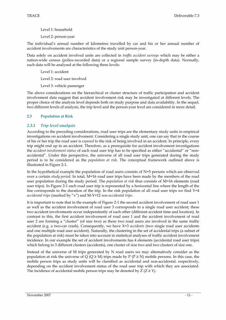
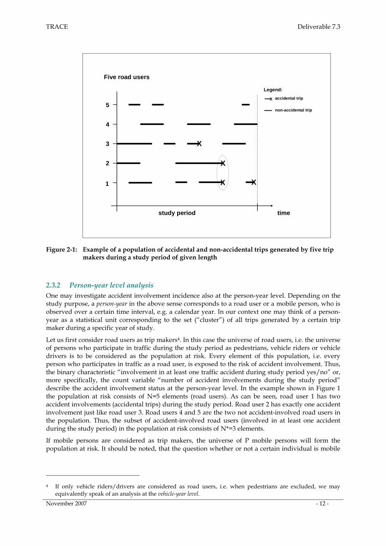
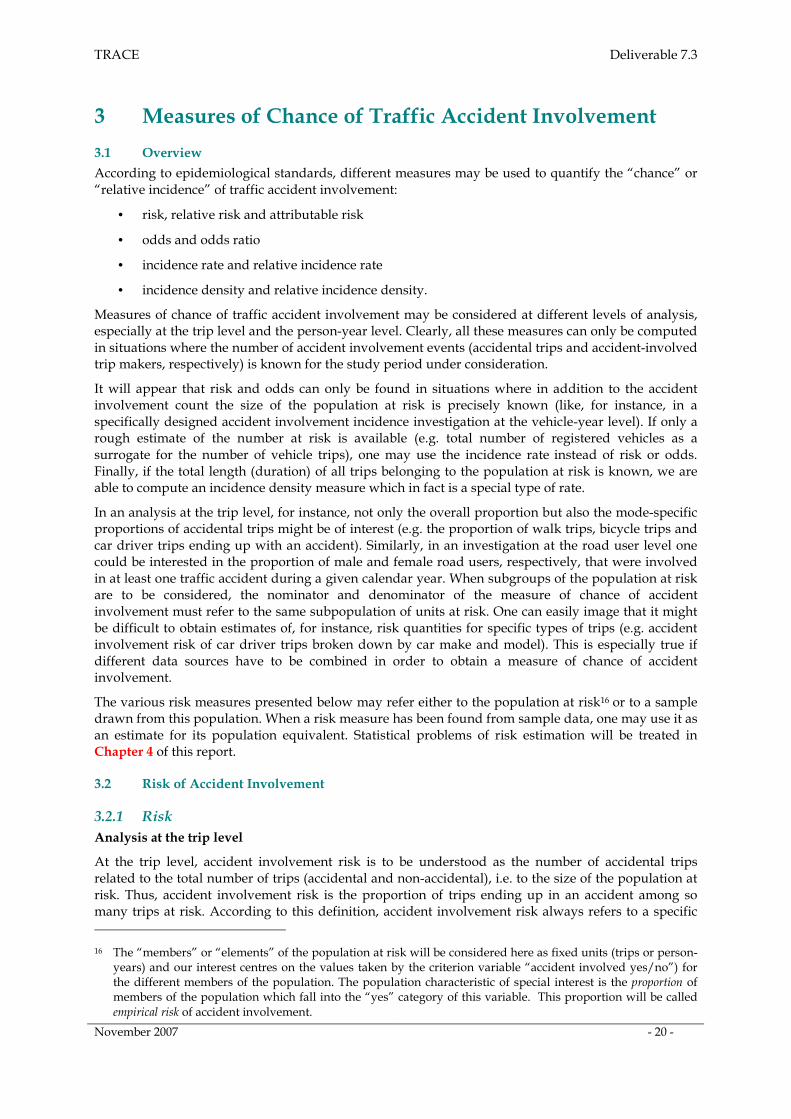
According to the preceding considerations, road user trips are the elementary study units in empirical investigations on accident involvement. Considering a single study unit, one can say that in the course of his or her trip the road user is exposed to the risk of being involved in an accident. In principle, every trip might end up in an accident. Therefore, as a prerequisite for accident involvement investigations the accident involvement status of each road user trip has to be specified as either “accidental” or “non-accidental”. Under this perspective, the universe of all road user trips generated during the study period is to be considered as the population at risk. The conceptual framework outlined above is illustrated in Figure 2-1.
In the hypothetical example the population of road users consists of N=5 persons which are observed over a certain study period. In total, M=16 road user trips have been made by the members of the road user population during the study period. The population at risk thus consists of M=16 elements (road user trips). In Figure 2-1 each road user trip is represented by a horizontal line where the length of the line corresponds to the duration of the trip. In the risk population of all road user trips we find Y=4 accidental trips (marked by “x”) and M-Y=12 non-accidental trips.
It is important to note that in the example of Figure 2-1 the second accident involvement of road user 1 as well as the accident involvement of road user 3 corresponds to a single road user accident; these two accident involvements occur independently of each other (different accident time and location). In contrast to this, the first accident involvement of road user 1 and the accident involvement of road user 2 are forming a “cluster” (of size two) as these two road users are involved in the same traffic accident (e.g. a two-car crash). Consequently, we have X=3 accidents (two single road user accidents and one multiple road user accident). Naturally, the clustering in the set of accidental trips (a subset of the population at risk) must be taken into account in statistical analyses of traffic accident involvement incidence. In our example the set of accident involvements has 4 elements (accidental road user trips) which belong to 3 different clusters (accidents), one cluster of size two and two clusters of size one.
Instead of the universe of M trips generated by N road users we may alternatively consider as the population at risk the universe of Q (Q ≥ M) trips made by P (P ≥ N) mobile persons. In this case, the mobile person trips as study units will be classified as accidental and non-accidental, respectively, depending on the accident involvement status of the road user trip with which they are associated. The incidence of accidental mobile person trips may be denoted by Z (Z ≥ Y).
TRACE Deliverable 7.3
November 2007 - 12 -
1
2
3
4
5
Five road users
study period time
X
X
X X
Legend:
accidental trip
non-accidental trip
X
Figure 2-1: Example of a population of accidental and non-accidental trips generated by five trip makers during a study period of given length
2.3.2 Person-year level analysis
One may investigate accident involvement incidence also at the person-year level. Depending on the study purpose, a person-year in the above sense corresponds to a road user or a mobile person, who is observed over a certain time interval, e.g. a calendar year. In our context one may think of a person-year as a statistical unit corresponding to the set (“cluster”) of all trips generated by a certain trip maker during a specific year of study.
Let us first consider road users as trip makers4. In this case the universe of road users, i.e. the universe of persons who participate in traffic during the study period as pedestrians, vehicle riders or vehicle drivers is to be considered as the population at risk. Every element of this population, i.e. every person who participates in traffic as a road user, is exposed to the risk of accident involvement. Thus, the binary characteristic “involvement in at least one traffic accident during study period yes/no” or, more specifically, the count variable “number of accident involvements during the study period” describe the accident involvement status at the person-year level. In the example shown in Figure 1 the population at risk consists of N=5 elements (road users). As can be seen, road user 1 has two accident involvements (accidental trips) during the study period. Road user 2 has exactly one accident involvement just like road user 3. Road users 4 and 5 are the two not accident-involved road users in the population. Thus, the subset of accident-involved road users (involved in at least one accident during the study period) in the population at risk consists of N*=3 elements.
If mobile persons are considered as trip makers, the universe of P mobile persons will form the population at risk. It should be noted, that the question whether or not a certain individual is mobile
4 If only vehicle riders/drivers are considered as road users, i.e. when pedestrians are excluded, we may equivalently speak of an analysis at the vehicle-year level.
TRACE Deliverable 7.3
November 2007 - 13 -
and thus belongs to the population at risk cannot be answered before the end of the study period5. Mobile persons with at least one accidental trip during the study period will be considered as accident-involved. The size of the subset of accident-involved mobile persons will be denoted by P*. As the values of the variables describing the accident involvement status of trip makers always refer to combinations of persons and study periods (years) it is reasonable to speak of an analysis at the person-year level.
2.3.3 Need for precise definition of the population at risk
According to Section 2.3.1 the population at risk, in general, is a universe of trips made by road users during a specific period of time. Depending on the purpose and design of the accident involvement study, one must define the population at risk in more detail. More specifically, the population at risk has to be delineated by factual, spatial and temporal characteristics.
Consider, for instance, an investigation where all crossings located in a study area are observed over a period of 3 months and where all motorized vehicle trips and all accidents involving motorized vehicles at these crossings are counted. This investigation is, of course, an analysis at the trip level and the population at risk is the set of trips satisfying at the same time the following three conditions: (1) trip is a motorized vehicle trip, (2) trip passes a crossing in the study area, and (3) trip is made during the 3 months study period.
As all trips having the characteristics (1) to (3) are registered, the investigation outlined above is a complete (100 percent) survey of the trips belonging to the population at risk.
2.4 Samples from the Population at Risk
A clear distinction has to be made between the target population (the population about we wish to draw conclusions), the study population (the specific population from which data are collected), and the sample (the subset of units selected from the study population on which data are actually obtained). Typically, researchers want to generalize their empirical results in a two-stage process: From the sample to the study population and then from the study population to the target population.
2.4.1 Sampling from a population of trips
Let us first consider traffic participation and accident involvement studies at the trip level. In this case the units at risk are trips, i.e. processes or events taking place in time and space. As these units are neither fixed subjects (like trip makers) nor objects (like vehicles), one cannot expect to have a complete register of the units at risk, i.e. a sampling frame, from which a simple random sample could be drawn. Frequently, not even the size of the population, i.e. the total number of units at risk will be known in practice. Therefore, in accident involvement studies at the trip level no simple random sampling of units (trips) from the complete population at risk is possible.
As an alternative to simple random sampling of trips one can think of a cluster sample design where person-days (primary units) are randomly selected and all trips (secondary units) made by the selected person on the selected day are recorded and classified as accidental and non-accidental, respectively. Although technically possible, this design appears not to be practical due to the extremely low frequency of accidental trips. In summary this means that the standard epidemiological survey, where one seeks information on the disease status (accidental versus non-accidental trip) and the risk factor status (e.g. age group of trip maker) of the sampled units at risk is not a realistic option for accident involvement risk analysis at the trip level.
Rather, in studies at the trip level the analyst is likely to have two independent samples, one sample of accidental trips (e.g. police-recorded accident involvements of road users) and a second sample of non-accidental trips (trips recorded in a general mobility survey). This data situation can be interpreted as follows: The population of all trips generated during the study period is subdivided
5 In a cohort study, the set of all persons selected for the study and followed up through time to record instances of accident involvement would form the universe of study units exposed to risk.
TRACE Deliverable 7.3
November 2007 - 14 -
into two disjoint strata - accidental and non-accidental trips - and from each stratum a sample6 is drawn. From an epidemiological point of view this corresponds to a so-called case-control study design with accidental trips as cases and non-accidental trips as controls (see Section 5.1.3).
Usually, the trip data set available to the analyst is merely a sample from the sub-population of accidental trips (e.g. police-recorded accident data). Obviously, no accident involvement risk study in the classical sense can be conducted under these circumstances as only cases but no controls have been observed. Sometimes, however, the concept of induced exposure may allow estimation of relative risks even under these adverse conditions (see Section 4.2.4).
2.4.2 Sampling from a population of person-years
For populations of persons and thus also for person-years complete registers exist from which units at risk can be drawn. In some countries all inhabitants are listed in a central register (e.g. Sweden) making simple random sampling possible; in other countries such registers exist at least at the community level (e.g. Germany) allowing multi-stage sampling of individuals. Similarly, if one is interested in accident involvement of motorized vehicles, the national vehicle register may serve as a complete list of the units at risk for an analysis at the vehicle-year level. From this register a simple or stratified random sample of vehicles can be drawn. Then, vehicle holders may be asked in an interview whether or not the selected vehicle was involved in a traffic accident during the study period (provided that the vehicle participated in traffic at all).
Summarizing it can be said that in accident involvement studies at the person-year or vehicle-year level simple or multi-stage random samples can normally be drawn from the complete population at risk. This offers the possibility to apply the full range of risk analysis methods which are suitable for epidemiological surveys. One must, however, be aware of the fact that due to the aggregate nature of person-year data the catalogue of risk factors to be assessed is substantially limited as compared to analyses at the trip level.
2.4.3 Sampling from an unspecified population at risk
Sometimes, a sample of accidental trips will be available where it is simply not clear to which population of trips this sample refers. Consider, for instance, a sample of hospital patients7 who were injured in a traffic accident. If there are several hospitals in the region to which victims can be brought after accident involvement, it will normally neither be possible to specify the corresponding population of victims nor to define the population at risk (Böhning, 1998, p. 38-40).
Another example of this type would be a sample of 9 accidents with 20 accident-involved vehicles which have been recorded at a certain crossing for a specific Tuesday. The process by which this data set has been generated may be interpreted as follows: For the crossing under consideration every Tuesday is to be considered as a primary unit to which Tuesday-accidents as secondary units and vehicles involved in Tuesday-accidents as tertiary units8 are assigned. Now, from the population of primary units (all Tuesdays) a sample of size 1 is selected (the specific Tuesday on which accidents are recorded) and the corresponding secondary and tertiary units are completely registered (no sub-sampling at the second and third stage). Ignoring for the moment that the accident-involved vehicles are grouped by collision (9 groups, each group corresponding to an accident), one could speak of a cluster sample of size 1 drawn from the universe of all “crossing-Tuesdays” and containing 20 study units. The selected cluster of 20 study units is, of course, a sample from the sub-population of accidental vehicle trips, not a sample from the complete vehicle trip population.
If, in addition to the mere registration of accidental vehicle trips (=accident-involved road users) all vehicle trips made at that crossing on the particular Tuesday were registered in a traffic count, the sample number of units at risk (vehicle trips at the crossing made on the particular Tuesday) would be
6 From the stratum of accidental trips even a 100-percent sample may be available, provided that police is recording actually all accidents.
7 Every hospital patient corresponds to an accidental person trip. 8 Of course, each tertiary unit corresponds to an accidental vehicle trip.
TRACE Deliverable 7.3
November 2007 - 15 -
known and the sample risk r (proportion of accidental trips among so many trips at risk) could be calculated. This sample value could then be used as an estimate of the population risk R which refers to all vehicle trips at that crossing on “comparable” Tuesdays.
2.5 Risk Factors
2.5.1 Risk factors as attributes of the units at risk
Basically, accident involvement studies at the trip level are dealing with the probability of a trip to end up in an accident, i.e. to be an accidental trip. Rarely, however, one is interested in the probability that an arbitrary trip from the population at risk is an accidental trip. Rather, one aims at evaluating the chance that a trip which possesses a certain attribute ends up in an accident. The probability of a trip being accidental given that the trip (or the corresponding trip maker) has the particular attribute under consideration is called the risk of accident involvement and the attribute considered is called risk factor. The trip maker attribute “insufficient driving experience” may serve as an example of a risk factor: car trips made by drivers who have this attribute are more prone to be accidental compared to car trips made by drivers having “sufficient driving experience”.
Those units at risk which have the attribute under consideration are said to be “exposed to the risk factor”9. Correspondingly, the units at risk which do not have the attribute considered are said to be “not exposed to the risk factor”. Frequently, the group without the risk factor will serve as a comparison group leading to the definition of the relative risk as the ratio of the risk of accident involvement for those with the risk factor to the risk of accident involvement for those without the risk factor. If the relative risk is above unity, then the factor under investigation increases risk; if less than unity it reduces risk. A factor which has a relative risk less than unity is referred to as a protective factor. Whereas “insufficient driving experience” is proven to be a factor which increases risk, the vehicle attribute “equipment with ESP” may be an example of a protective factor.
Remark: The meaning of the epidemiological term “factor” (risk factor or protective factor) is different from the meaning of this term in analysis of variance (ANOVA). In the ANOVA terminology a “factor” is a categorical explanatory variable which might affect the distribution of a certain criterion variable. The possible values of a factor are called “levels”. Thus, a risk factor in the epidemiological sense is a specific level of a factor according to the ANOVA terminology.
In this report the term “risk factor” always refers to a specific level of the explanatory variable “risk factor status”. In an ANOVA context, one would, for instance, say that the factor “driving experience status of trip maker” is measured at two levels: “insufficient driving experience” and “sufficient driving experience”. In epidemiology, the trips belonging to the first category are said to be those with the risk factor whereas the trips belonging to the second category are said to be those without the risk factor “insufficient driving experience”. Alternatively, one may speak of those exposed and those not exposed to the risk factor “insufficient driving experience”.
In empirical studies on the determinants of accident involvement, the population at risk will be broken down by various characteristics of the trip maker (e.g. age group) and the trip itself (e.g. trip purpose) in order to investigate whether or not these characteristics10 are associated with the incidence of accident involvement. From this type of exercise one arrives, for instance, at the descriptive finding
9 Every trip, of course, is exposed to the risk of ending up in an accident. Thus, the wording “to be exposed to risk” is a synonym for “being a member of the population at risk”. The probability of an arbitrary trip (i.e. without imposing any conditions on the characteristics of the trip) to be accidental may be termed average risk. Normally, the accident involvement risk of a trip made by a person who is exposed to the risk factor “insufficient driving experience” will be above average. As can be seen, a clear distinction has to be made between exposure to risk and exposure to a risk factor. Whereas “exposure to risk” describes the fact that any trip may end up in an accident, “exposure to a risk factor” means that a given trip has a certain attribute which is considered as a risk factor in the sense that the corresponding accident involvement risk is above average.
10 Every such characteristic corresponds to a specific risk factor status variable.
TRACE Deliverable 7.3
November 2007 - 16 -
that young drivers are more prone to accident involvement than middle-aged or elderly drivers. This finding may lead to an investigation of why this should be so, i.e. to a study of the causal factors or the determinants of accident involvement.
2.5.2 Measuring risk factors
The risk factor status of a unit at risk is frequently measured at only two levels: “exposed” and “not exposed”. One may, however, also have a set of possible categorical or ordinal outcomes of the risk factor status11. A typical example would be the trip characteristic “trip purpose” with levels work, business, shopping, leisure and the like. In this situation one would choose one level of the risk factor status to be the base level and compare all other levels to this base. Choosing, for instance, “work trip” to be the base level one might find that the relative risk of “leisure trip” is above unity; consequently, “trip-making for leisure purposes” could be considered to be a risk factor.
Risk factor status may also be a continuous variable12 or a discrete variable with a large number of outcomes. In this case the risk factor status can be grouped; one may, for instance, consider age groups instead of the variable “age in years”. Grouping, of course, leads to loss of information on risk factor status.
Both from a conceptual and technical point of view, many risk factors have the common feature that they can be measured in several different ways. For instance, the trip- and driver-related characteristic “driving under the influence of alcohol” may be measured precisely by a blood alcohol test or simply by asking the driver whether or not he or she has consumed alcohol prior to the trip. Frequently, the possibilities of assessing risk factors are limited by the fact that the characteristics recorded for accidental trips are not identical with the characteristics recorded for non-accidental trips. For instance, whereas in practically all mobility surveys the purpose of the trip is coded, this is not the case in many accident data collection systems.
2.6 Investigating Traffic Accident Causation
Traffic accident causation may be investigated in several different ways. Among the candidate methodologies for empirical accident causation studies the following two concepts are of special relevance:
• Direct or “case-by-case” approach: Accident causes attributed to registered accidents and road users involved by expert judgement
• Indirect or “statistical” approach: Accident causes as statistically proven risk factors for accident involvement
These two approaches which complement one another are described subsequently.
2.6.1 Accident cause as a measurable characteristic of accidents and road users involved
According to this concept, accident causes are considered to be the possible values of a measurable nominal variable “accident cause” which can be defined both at the accident and road user level.
• At the accident level, this variable is usually termed “general accident cause”. Subsequently, the symbol A is used to denote this variable; the values (categories) of A are the specific general accident causes Ai (i=1, 2, …).
• At the road user level, the variable under consideration is normally called “road user-related accident cause”; in the sequel, the symbol B will be used to denote this variable. The possible values of B are denoted by Bj (j=1, 2, …). The variable values Bj are called specific road user-related (or person- and vehicle-related) accident causes.
11 In epidemiology one speaks in this case also of a risk factor measured at several levels. This is not fully consistent as normally “risk factor” denotes a single level of the variable risk factor status.
12 In epidemiology, the term continuous risk factor is used.
TRACE Deliverable 7.3
November 2007 - 17 -
• Typically, more than one cause can be attributed to the accident and the road user involved (multiple responses).
To each recorded accident, i.e. case by case, the value of the directly measurable nominal variable “general accident cause“ is attributed by expert judgement – provided that a specific general accident cause applies to the accident under consideration. Similarly, one or more specific road user-related accident causes are attributed to each road user involved – provided that the expert considers the road user as “responsible” for the accident13. For accidents (road users) to which no specific general (road user-related) accident cause can be attributed, the value of the variable A (B) is missing.
Obviously, most police-recorded accident data sets rely on this concept: proceeding from his or her personal judgement, the police officer recording the accident describes the causes of the accident in the survey form according to a given list of possible causes. Typically, in-depth accident data sets also contain general and road user-related accident cause variables which are measured in the way described above; in this case the “expert” is not a police officer but a member of the accident research team.
The values Ai of the variable “general accident cause” are categories like “insufficient road lighting” and “heavy rain”. Typical examples for the values Bj of the variable “road user-related accident causes” are “unadapted speed” and “driving under the influence of alcohol”. Usually, the road user mainly responsible, i.e. the person chiefly to blame for the accident, is identified by expert judgement. This additional variable, among other things, opens the possibility for investigations based on the concept of “induced exposure”.
In an empirical accident causation study based on the concept of directly measured accident causes, one may, for instance,
• arrange specific accident causes according to the frequency of occurrence
• investigate the association between accident cause and other characteristics of the accident and the road users involved (e.g. accident cause and accident outcome severity)
• identify those groups of accidents and accident-involved road users which are prone to specific accident causes like, for instance, improper behaviour towards pedestrians.
Depending on the purpose of the study, the aforementioned accident cause variables A and B can be considered both as dependent and explanatory variables in accident causation analyses. In an empirical accident causation study at the road user level conducted solely on the basis of accident data, one may, for instance, assess the factors determining the probability14 of being blamed for causing an accident due to unadapted speed (“unadapted speed yes/no” as dependent variable). On the other hand, one could, for instance, investigate the effect of the explanatory variable “unadapted speed yes/no” on injury severity of the road user itself or on injury severity of the opponent of the road user under consideration.
If external exposure quantities like total trip volume or total vehicle mileage are available, one may investigate the unconditional accident causation risk, i.e. the risk of being involved in an accident and blamed for initiating the crash. In this situation, the “population at risk” consists of all road user trips and the subpopulation of accidental trips is further classified into “responsible accidental” and “nonresponsible accidental” trips. From an epidemiological point of view this corresponds to the situation where the disease variable (in our case: accident involvement status) is measured at three levels: no involvement, involvement as nonresponsible road user and involvement as responsible road user.
The direct or case-by-case approach to accident causation may, of course, be criticised due to the possible subjectivity of expert judgements. If several experts were asked to attribute accident causes retrospectively to a given accident or road user involved, it may well be that they will render different judgements although they were provided with exactly the same information about the accident (e.g. police and hospital files). Similarly, if the assignment of specific accident causes is based on
13 In cases where two or more road users are involved in the same accident, usually the “mainly responsible” road user is also identified. 14 Conditional on accident involvement of the road user
TRACE Deliverable 7.3
November 2007 - 18 -
interviewing accident involved parties or witnesses of the accident one may obtain non-objective results.
Remark: Traffic accident registers kept by police or insurance companies where the cause(s) of the accident are recorded are an important source of routine data for accident causation studies. This is perfectly comparable with the situation in epidemiological research in general, where the use of routine mortality data derived from death certificates is common practice.
By law, a certificate is completed whenever a death occurs. This is done at a local registration centre where births and marriages will also be recorded. On the death certificate characteristics such as gender, age at death and place of residence along with the cause of death are recorded. The latter uses the International Classification of Diseases (ICD) codes. Normally, both the underlying and the associated causes of death are recorded. See Woodward (1999), p. 20-22.
Obviously, from a purely methodological point of view there is a correspondence between death registers and accident registers as sources of data on the causes of the event of interest15.
2.6.2 Accident causes as proven risk factors for accident involvement
Accident determinants or accident causes, in general, are factors that precipitate accident occurrence. Therefore, the concept of accident involvement risk appears to be a quite natural methodological framework for empirical accident causation studies. When risk analysis methods are to be applied, no empirically observed accident cause variables in the above sense are required. Rather, the determinants of accident involvement, i.e. the risk factors for accident involvement are regarded as “accident causes”, provided that the corresponding factors are sufficiently strong correlated with accident involvement.
Under the indirect approach accident causes are always explanatory variables. Moreover, the approach may be characterised as “statistical” rather than case-by-case. Clearly, as accident involvement is the dependent variable, such an indirect analysis of accident causation requires both accident and exposure data, i.e. data on accidental and non-accidental trips or, alternatively, data on accident-involved and accident-free road users.
Under this concept, trip-related and road user-related attributes which significantly affect the probability of accident involvement can be identified as risk factors or “accident causation factors”. In view of the type and content of the databases available, one must, however, be aware of the fact, that the empirical findings thus obtained may only be descriptive rather than causal: whether or not such a risk or accident causation factor is a “true aetiological agent” must be checked carefully.
For instance, the finding that young drivers are more prone to traffic accident involvement will lead to investigation why this should be so. Obviously, juvenility as such is not a causal factor for accident involvement but only an indicator of increased accident proneness. Frequently, the actual accident causes like risk propensity and lack of driving experience are latent variables (i.e. variables which have not been observed in the survey under consideration) correlated with the observed indicator juvenility. This feature of the indirect approach limits its range of applicability in accident causation studies.
2.6.3 Statistical analysis methods for accident causation studies
Although the two approaches to accident causation analysis described in Section 2.6 differ fundamentally from a conceptual point of view, it appears that largely the same statistical models (discrete regression models of various types) can be used to assess the determinants of accident causes and accident involvement, respectively.
Once the general and road user-related causes of a registered accident have been determined by expert judgement and added to the accident data set, it is of interest to identify those accident- and road user-related characteristics which are closest correlated with the occurrence of specific accident
15 Death registers, however, will normally be more complete than accident registers.
TRACE Deliverable 7.3
November 2007 - 19 -
causes. For this type of statistical analysis, discrete regression models (e.g. of the logit or probit type) are appropriate. As usual, model specification is mainly determined by the scaling of the dependent variable. The models may be equally applied to datasets of individual (micro level, i.e. one record per accident-involved road user) and aggregate data (multidimensional contingency tables). If, as usual, the dataset contains information on road users involved in the same accident, model specification should normally take account of this “clustering” by applying, for instance, random effects models.
Under the indirect approach, the risk factors determining accident involvement are to be assessed in order to identify general and road user-specific traffic accident causes. For individual data, binary regression models (e.g. of the logit and probit type) are suitable. As usual, the proper specification of the model depends on the design of the study (accident involvement survey, cohort study, case-control study). For aggregate data various types of generalized linear models can be used.
TRACE Deliverable 7.3
November 2007 - 20 -
3 Measures of Chance of Traffic Accident Involvement
3.1 Overview
According to epidemiological standards, different measures may be used to quantify the “chance” or “relative incidence” of traffic accident involvement:
• risk, relative risk and attributable risk
• odds and odds ratio
• incidence rate and relative incidence rate
• incidence density and relative incidence density.
Measures of chance of traffic accident involvement may be considered at different levels of analysis, especially at the trip level and the person-year level. Clearly, all these measures can only be computed in situations where the number of accident involvement events (accidental trips and accident-involved trip makers, respectively) is known for the study period under consideration.
It will appear that risk and odds can only be found in situations where in addition to the accident involvement count the size of the population at risk is precisely known (like, for instance, in a specifically designed accident involvement incidence investigation at the vehicle-year level). If only a rough estimate of the number at risk is available (e.g. total number of registered vehicles as a surrogate for the number of vehicle trips), one may use the incidence rate instead of risk or odds. Finally, if the total length (duration) of all trips belonging to the population at risk is known, we are able to compute an incidence density measure which in fact is a special type of rate.
In an analysis at the trip level, for instance, not only the overall proportion but also the mode-specific proportions of accidental trips might be of interest (e.g. the proportion of walk trips, bicycle trips and car driver trips ending up with an accident). Similarly, in an investigation at the road user level one could be interested in the proportion of male and female road users, respectively, that were involved in at least one traffic accident during a given calendar year. When subgroups of the population at risk are to be considered, the nominator and denominator of the measure of chance of accident involvement must refer to the same subpopulation of units at risk. One can easily image that it might be difficult to obtain estimates of, for instance, risk quantities for specific types of trips (e.g. accident involvement risk of car driver trips broken down by car make and model). This is especially true if different data sources have to be combined in order to obtain a measure of chance of accident involvement.
The various risk measures presented below may refer either to the population at risk16 or to a sample drawn from this population. When a risk measure has been found from sample data, one may use it as an estimate for its population equivalent. Statistical problems of risk estimation will be treated in Chapter 4 of this report.
3.2 Risk of Accident Involvement
3.2.1 Risk
Analysis at the trip level
At the trip level, accident involvement risk is to be understood as the number of accidental trips related to the total number of trips (accidental and non-accidental), i.e. to the size of the population at risk. Thus, accident involvement risk is the proportion of trips ending up in an accident among so many trips at risk. According to this definition, accident involvement risk always refers to a specific
16 The “members” or “elements” of the population at risk will be considered here as fixed units (trips or person-years) and our interest centres on the values taken by the criterion variable “accident involved yes/no”) for the different members of the population. The population characteristic of special interest is the proportion of members of the population which fall into the “yes” category of this variable. This proportion will be called empirical risk of accident involvement.
TRACE Deliverable 7.3
November 2007 - 21 -
population of trips at risk generated by certain universe of “trip makers” (road users and mobile persons, respectively) during a specified period of time.
Considering road users as trip makers, the trip-related accident involvement risk is defined as
(3.1) RT = Y/M = number of accidental trips / number of trips at risk.
Obviously, the risk RT is simply the proportion of accidental trips among all trips generated by the road user universe under consideration during the study period. In our numerical example we have RT = 4/16 = 0.25. This means that 25 percent of all road user trips during the study period are accidental trips. In studies where mobile persons are considered as trip makers the trip-related accident involvement risk would be defined as RT = Z/P.
In a purely descriptive analysis referring to the complete population at risk or to a concrete sample from this population, the “empirical” risk (3.1) is frequently also called cumulative incidence rate (CIR). The term “risk” may then be reserved for the probability of the event that an arbitrary trip is an accidental trip. In this report the empirical population risk is always denoted by the capital letter R. Sample values that are estimates of their population equivalents are denoted by the lowercase letter r. See also Chapter 4.
Analysis at the person-year level
At the person-year level we may define accident involvement risk as the ratio of two counts, namely, the number N* of accident-involved road users and the total number N of all road users exposed to accident involvement risk during the study period of one year:
(3.1a) RP = N*/N.
In our numerical example we have RP = 3/5 = 0.6, i.e. 60 percent of the road users observed over the study period are involved in at least one traffic accident.
In real-world situations multiple accident involvement of a specific road user during a study period of standard length (e.g. one calendar year) is a rare event. Therefore, N* will normally be only slightly smaller than the number of accidental trips Y. On the other hand, the total number M of road user trips will normally be considerably larger than the number N of road users (about 1’000 trips per road user and year). In practice, therefore, the numerical value of the trip-related accident involvement risk RT will be by far smaller (factor 1/1’000) than the accident involvement risk RP at the person-year level.
If, more generally, mobile persons are considered as trip makers, the accident involvement risk at the person-year level is defined as P*/P; this risk quantity may be interpreted as the proportion of mobile persons (vehicle users and pedestrians) from a certain human population who were involved in at least one road traffic accident in the course of a one-year study period.
It should be reminded that all empirical risk quantities introduced above are proportions in the sense that the numerator is part of the denominator. Thus, the traffic accident involvement risks RT and RP always lie between 0 and 1. The other three measures of chance of accident involvement incidence (odds, rate and density) do not have this property.
3.2.2 Relative risk
If in an analysis at the trip level the population of trips at risk is subdivided according to a certain characteristic (e.g. age of vehicle used for trip-making) into two groups 1 and 2 (e.g. trips made by old and new vehicles, respectively) the group-specific risks are defined according to (3.1). Given the two group-specific risks, the relative risk of accident involvement for trips belonging to group 2, compared to those belonging to group 1, is given by
(3.2) Λ = RT2/RT1.
If more than two groups are distinguished (risk factor measured at several levels), one group (e.g. group 1) may be considered as the reference group (also termed base group) and the analyst may relate the risk of the other groups to that of the reference group.
The Greek letter Λ (lambda) represents the population relative risk. Its estimate in a sample will be denoted by the lowercase letter lambda (λ).
TRACE Deliverable 7.3
November 2007 - 22 -
3.2.3 Attributable risk
The relative risk, of course, tells nothing about the overall importance of a certain risk factor. This is because it does not take into account how the units at risk are distributed over the different categories of the risk factor status variable. Let in the example of Section 3.2.2 the accident involvement risk for trips made by new cars (the “unexposed” group of units) be denoted by RT1 and the overall accident involvement risk by RT. In the hypothetical situation where all old cars were substituted by new cars, exposure to the risk factor “trip-making using an old car” would no longer be present and all members of the population at risk would experience the risk of the unexposed group (i.e. RT = RT1).
Thus, the difference RT - RT1 may be interpreted as the absolute increase in overall population risk due to the fact that some trip makers use old cars instead of new ones. Similarly, the ratio RT1/RT tells the analyst something about the percentage reduction in population risk if exposure to the risk factor was completely removed. Consequently, the difference θ = 1 - RT1/RT denotes the proportion of the observed overall population risk RT which can be attributed to the risk factor “trip-making using an old car”. If, for instance, the difference takes on the value θ = 0.22, this would mean in our example that 22% of the overall risk of accident involvement is attributed to driving an old car instead of a new vehicle.
In epidemiology, the quantity
(3.3) θ = 1 - RT1/RT = (RT - RT1)/RT
is termed attributable risk. The attributable risk tends to be large,
• if the risk factor under consideration is rare provided the relative risk is high or
• if the relative risk is low provided the risk factor is common.
“Attributable” does not imply causation. In the above example one could, for instance, conclude that 22 % of the cases of accident involvement would be removed, if all drivers of old cars would switch to new cars. This, however, would be over-optimistic if there is a third (“confounding”) factor involved which determines both vehicle choice (old versus new) and accident involvement. Age of driver could, for instance, be such a confounder.
3.3 Odds of Accident Involvement
3.3.1 Odds
At the trip level, the chance of accident involvement can also be measured by relating the number of accidental trips to the number of non-accidental trips:
(3.4) ΩT = Y/(M-Y).
This measure is called the odds of accident involvement and is to be understood here as a population value. In our hypothetical example we have ΩT = 4/(16 - 4) = 4/12 = 0.33. This result tells us that the number of accidental trips is just one third of the number of non-accidental trips, i.e. non-accidental trips are three times more frequent than accidental trips.
The odds of accident involvement may, of course, also be defined at the person-year level:
(3.4a) ΩP = N*/(N – N*).
In our example we find ΩP = 3/(5 – 3) = 3/2 = 1.5, i.e. the number of accident-involved drivers exceeds the number of not involved (accident-free) drivers by 50 percent.
3.3.2 Odds ratio
If group-specific odds, i.e. odds of accident involvement for units (trips or person-years) belonging to group 1 and group 2, respectively have been determined, the odds ratio for units belonging to group 2, compared to units belonging to group 1, is given by
(3.5) Ψ = Ω2 /Ω1.
TRACE Deliverable 7.3
November 2007 - 23 -
The Greek letter Ψ (psi) is used in this report to denote the population odds ratio. In later sections, a sample value that is an estimate of the population odds ratio will be denoted by the lowercase letter ψ.
3.4 Accident Involvement Rate
3.4.1 Rate
In quite many analyses at the trip level one knows the number Y of accidental trips but not the total number M of trips. Similarly, in an analysis at the person-year level one may know rather precisely the number N* of trip makers who had an accident but has no information on the number N of trip makers at risk. In both cases we know the numerator but not the denominator required to determine the risk of accident involvement.
If we have at least a rough estimate M0 of the size of the population at risk or any other quantity to which the number of accident involvement events can be related in a meaningful way, we may use the corresponding quotient to measure the chance of accident involvement. Any quotient of the form
(3.6) ρ = Y/M0
is called accident involvement rate.
3.4.2 Types of accident involvement rates
Well known examples of accident involvement rates are
• the per-capita accident involvement rate for analyses at the person-year level (Y = annual number of accidental person trips; M0 = mid-year population) and
• the per-vehicle accident involvement rate for analyses at the vehicle-year level (Y = annual number of accidental vehicle trips; M0 = mid-year vehicle stock).
If the study period covers T years, the total number Y of accidental person and vehicle trips should be related to the total number Z of person- or vehicle-years for this period. In the simplest case we may determine the denominator of the rate Y/Z as follows: Z = M0(1) + M0(2) + … + M0(T), where M0(t) is the mid-year vehicle stock for year t (t=1,…,T).
When dealing with rates it is often assumed that the accident involvement count Y is a random variable whereas the denominator M0 is assumed to be a fixed known quantity. If the accidents involvement events would occur randomly and independently, it would be reasonable to assume that their number Y follows a Poisson distribution (see Woodward, 1999, p. 137-139). Due to the cluster structure described in Section 2.3 it is, however, more appropriate to apply stochastic models accounting for “over-dispersion” (see McCullagh and Nelder, 1992, p. 193-208). Details can be found in Section 4.3.
3.4.3 Relative rate
To compare two rates one can use the relative rate, group 2 compared to group 1, which is given by
(3.7) ρrel = ρ2/ρ1 = (Y2/M02) / (Y1/M01).
A statistical approach to estimate confidence limits for the relative rate can be found in Woodward, 1999, p. 139-140.
3.5 Accident Involvement Density
Obviously, the characteristic “duration of trip” - which under a different perspective may also be termed “traffic participation time under risk” - varies in the population of trips. Similarly, the “total person-time under risk” corresponding to the total duration of all trips made by a given person during the study period varies in the population of trip makers. The phenomenon of non-constant time under risk (non-constant risk exposure time) for the elements of the population at risk is quite common in epidemiological research and leads to the epidemiological concept of “incidence density”.
TRACE Deliverable 7.3
November 2007 - 24 -
3.5.1 Time-related accident involvement density
Let t(i, j) denote the duration of the j-th trip of person17 i during the study period (i=1,…,N; j=1,…,m(i)). Then, T(i) = Σ t(i, j) where summation is made over the index j is the total person-time under risk of person i. Summation over the index i finally yields the overall total person-time under risk T = Σ T(i), which corresponds to the total traffic participation time spent by all members of the population during the study period.
For a given population of trip makers the time-related accident involvement density is defined as the ratio of incidence of accidental person-trips and total person-time under risk:
(3.8) δtime = Y / T.
The denominator T is considered as an “aggregate measure of exposure” that can be used to normalise the incidence of accident involvement Y. In our context this risk concept is especially reasonable because at every moment in time, while participating in road traffic, the possibility of accident involvement exists.
In our numerical example we may assume that the overall total T of the trip characteristic “duration of trip” is 480 minutes or 8 hours (corresponding to a mean trip duration of 480/16 = 30 min per trip). Under this assumption we obtain the time-related accident involvement density δtime = 4/8 = 0.5. This measure tells us that on average there are 0.5 accident involvements of persons per person-hour of traffic participation (fortunately, real-world incidence densities are by far lower).
3.5.2 Distance-related accident involvement density
At every spatial point in the road network which is passed by a person while participating in traffic an accident may happen. When person trips are considered as study units we may, therefore, also use “trip length” or “travel distance under risk” d(i, j) as an appropriate measure of traffic accident involvement risk exposure. Thus, the total person-distance under risk D generated by the population of trip makers during the study period may serve as a standard for comparison.
This concept leads to the distance-related accident involvement density as a relative measure of accident involvement incidence:
(3.9) δdistance = Y/D
Under the assumption that in our hypothetical example the total person-distance under risk equals D = 240 km (i.e. mean trip distance 240/16 = 15 km per trip), the distance-related traffic accident involvement density is δdistance = 4/240 = 0.0167 accident involvements of persons per person-kilometre of traffic participation.
In general, we may denote the accident involvement density by
(3.10) δ = Y/X,
where X represents the population total of a suitable exposure characteristic of the units at risk.
3.5.3 Relative density
To compare two densities one can use the relative density, group 2 compared to group 1, which is given by
(3.11) δrel = δ2/δ1.
In the epidemiological literature the relative density is also called incidence desity ratio (IDR).
3.6 A Note on the Differences between Risks, Odds, Rates and Densities
The various measures of chance of accident involvement as introduced in Sections 3.1 to 3.5 are all deterministic measures referring to a particular well-defined finite population at risk. The numerical
17 Depending on the analysis level chosen the “persons” under consideration may be road users or in a broader sense mobile persons (road users together with vehicle passengers).
TRACE Deliverable 7.3
November 2007 - 25 -
values of these measures can be obtained by surveys or some other types of study. Except for very specific populations at risk, it will not be possible to conduct a complete census yielding the true or exact value of the measure under consideration. Rather, some type of sampling from the population at risk will provide data which allow the measure of chance to be estimated.
For instance, the sample value r of accident involvement risk presented in the subsequent Section 4.1 is to be interpreted 18 as an estimate of the corresponding population risk R. Clearly, both the population and the sample risk are proportions. But whereas R is a fixed (but unknown) quantity, the sample risk r is a random variable. Obviously, odds, rates and densities as defined in Sections 3.3 to 3.5 are not proportions. Therefore, these quantities are measures of chance but may not be interpreted as “risk” quantities in the above narrow sense. The only exception to this rule is the accident involvement rate ρ which under favourable circumstances might be a good approximation to the population risk R.
Calculation of both the risk and the odds of accident involvement require precise knowledge of the size of the population at risk. It should be noted, that the odds are rarely of interest as the risk is the generally preferred measure of chance. However, in studies on the comparative chance of accident involvement the odds ratio has at least the same importance as the relative risk - either because the odds ratio is all we can estimate (e.g. in case-control studies) or is the more convenient to calculate (e.g. in logistic regression analysis).
As already noted, the accident involvement density (e.g. δtime) is not a proportion (δtime > 1 is possible). Rather, it is a ratio of two population characteristics (number of accidental trips related to the total duration of all trips under risk). Therefore, δtime may not be interpreted as a risk quantity in the above sense: Density is not a measure of accident involvement “risk” but a measure of accident involvement “intensity”. It expresses the incidence of accident involvement per unit of a certain risk exposure quantity, especially the number of accident involvements per hour or per kilometre of traffic participation. As the duration and length of the units at risk varies, density measures are appropriate measures of chance of accident involvement. Formally, there is no difference between the sample values of densities and rates as both measures are quotients of a random variable and a quantity usually assumed to be fixed and known. Conceptually, however, a clear distinction can be made: the denominator T and D, respectively, of the accident involvement density is the population total of a characteristic of the units under risk, whereas the denominator M0 of the accident involvement rate typically is an estimate of the size M of the population at risk.
Not surprisingly, different statistical models have to be applied when the different measures of chance of accident involvement are to be estimated (rates and densities, however, may be estimated and analysed using the same models). Various statistical models for the analysis of data from accident involvement studies are presented in the subsequent chapter.
18 An alternative interpretation of r would be that of an estimate of the probability of accident involvement.
TRACE Deliverable 7.3
November 2007 - 26 -
4 Statistical Models for Alternative Measures of Chance of Accident Involvement
4.1 Criteria for Choosing a Statistical Model for the Measure of Chance
When choosing a statistical model, the type of study and the nature of the data to be analysed must be taken into account. In addition, the aims of data analysis (e.g. parameter estimation or hypothesis testing) play an important role. Although different types of traffic accident involvement studies will be treated in detail not till Chapter 6, some basic statistical models can already be presented at this stage.
If we look at the different sample measures19 of chance of accident involvement, namely,
risk = y/m odds = y/(m-y) rate = y/m0 density = y/x
where m = total number of units at risk in the sample, y = number of accident-involved units, m0 = external estimate of m and x = sum of an exposure variable (summed over the m units at risk), it is evident that the choice of the measure of chance and the corresponding statistical model depends on criteria like the following:
• Are y and m (and/or x) known from a single data source (micro or aggregate data)?
• May y and m (and/or x) be determined from two different micro or aggregate data sources?
• Has y been determined from a single sample of size m drawn from the population at risk?
• Have m, y and x been determined from a planned study of the cohort or case-control study type?
• May m be determined at all? If not, is an estimate m0 from external sources available?
Subsequently, the binomial distribution (as a model for the risk r) and the Poisson distribution (as a model for the accident involvement count y) will be presented.
4.2 Models for Risk and Relative Risk
4.2.1 A binomial model for traffic accident involvement risk
At the trip level, accident involvement as the criterion variable of a risk study is a dichotomous characteristic: Trips may be either accidental or non-accidental. When a sample of m trips from the population is obtained in one way or another, we may count the number of accidental trips thus finding the sample incidence y of the event of interest (y = 0, 1,…, m) and the sample risk r = y/m. Formally, the same type of incidence data would be obtained when person-years or vehicle-years were classified as either accident-involved or not and the number of accident-involved units among a given total number of units is counted.
In the person- or vehicle-year example one can easily image that the units are selected from a register according to a simple random sampling procedure. In this case, the binomial distribution would be an appropriate model for the count y. Using, for instance, the national vehicle register as a sampling frame we may draw a simple random sample of m vehicles from the complete set of M vehicles registered in the country under consideration. If the vehicle holders were asked in a survey to report whether or not the selected vehicle was involved in an accident during the last twelve months, the population risk R = Y/M could be estimated by the sample risk r = y/m, where y denotes the number of accident-involved vehicles in the sample (y = 0, 1, …, m).
As under simple random sampling the denominator m of the sample risk is fixed and the numerator y follows a binomial distribution, the lower and upper limit of a confidence interval for the fixed and
19 In these measures the counts m, y and m0 and the trip time or distance total x must, of course, refer to the same basic group of study units.
TRACE Deliverable 7.3
November 2007 - 27 -
unknown population risk R can also be estimated. If the binomial distribution of y is approximated by a normal distribution, an approximate (1-α)·100 per cent confidence interval for R is given by
(4.1) r ± z1-α/2 √r(1-r)/m.
From (4.1) we obtain an interval, of which we can be confident that it will cover the unknown population risk R, i.e. the unknown proportion of vehicles in the country that were involved in at least one traffic accident within the study year.
It should, however, be noted that the confidence interval (4.1) may be fairly inaccurate due to the fact that typically the risk of accident involvement is rather small. Thus, alternative methods of estimating confidence intervals for a binomial proportion as described in Fleiss (1981) and Vollset (1993) should be considered by the analyst.
Since no register of trips exists from which a sample could be selected, the binomial model seems hardly to be applicable in studies at the trip level. Although, in principle, a multi-stage sampling procedure would be possible to obtain information on individual trips in a combined traffic participation and accident involvement survey, this design will play no major role in practice: Due to the fact that accident involvement is an extremely rare event it seems not to be efficient to conduct, for instance, a household mobility survey where in addition to the usual trip characteristics the accident involvement status of the trips has to be reported.
4.2.2 A normal distribution model for the log of the relative risk
In order to obtain a confidence interval for the population relative risk Λ = R2/R1 it is necessary to know the standard error of λ or log λ, where λ is the sample relative risk. It can be shown that log λ asymptotically follows a normal distribution20 with mean log Λ and Var(log λ) estimated by21
(4.2) Var*(log λ) = 1/y2 -1/m2 + 1/y1 -1/m1,
In equation (4.2) m1 and m2 denote the total number of units selected from groups 1 and 2, respectively and y1 and y2 denote the number of accidental units found in the sample drawn from group 1 and 2, respectively. Using these results, the lower and upper limits Llog and Ulog of a confidence interval for log Λ can be calculated in the usual way. The confidence interval for the population relative risk Λ itself is then obtained by raising the two limits to the power e:
(4.3) L = exp Llog and U = exp Ulog.
For details and numerical examples see Woodward (1999), p. 108-111.
Frequently, the two groups correspond to the outcomes of a certain risk factor status variable. In this situation the base or reference group (group 1) is normally taken as “absence of the risk factor”. For instance, in order to assess the risk factor “male trip-maker” in a study at the person-year level, one would relate the risk of male trip-makers (numerator) to the risk of female trip-makers (denominator). In this example the trip-maker attribute of being male would be considered to be a “true” risk factor for accident involvement if the lower limit L of the confidence interval for the relative risk is above unity.
4.2.3 A normal distribution model for the attributable risk
As with the risk and relative risk, there are various statistical methods for calculating approximate confidence intervals for the attributable risk θ = (R - R1)/R. Again, an application of these methods requires empirical data obtained by sampling from the population at risk. The interested reader is referred to Woodward (1999), p. 132-137.
20 The distribution of the sample relative risk λ* is skewed and a logarithmic transformation is necessary to ensure approximate normality.
21 It is assumed here that m1 and m2 are fixed sample sizes. This assumption holds for cohort studies. For surveys where m1 and m2 are not fixed but random, we can estimate the variance of log λ* conditional on the sample actually obtained.
TRACE Deliverable 7.3
November 2007 - 28 -
4.2.4 Logistic regression models for accident involvement risk
If we are not merely interested in estimating the population value R of accident involvement risk but also in assessing different risk factors, logistic regression models are appropriate if a simple random sample from the population at risk has been drawn or if the data arise by cohort study22. In analyses at the person- or vehicle-year level, a logistic regression model represents the dependence of accident involvement risk (as a probability) on risk factor status variables like age of trip-maker and annual sum of hours spent travelling or engine power and annual mileage of vehicle, respectively. Whenever units with different accident involvement status can be found in the sample and when risk factor status varies over the units, one can answer the question whether or not a certain risk factor (e.g. being a male trip-maker) significantly affects the chance of being involved in an accident.
When specifying logistic regression models for the dichotomous criterion variable “accident involvement status (yes/no)”, a distinction has to be made between
• binary risk factors,
• quantitative risk factors,
• categorical risk factors and
• ordinal risk factors.
Moreover, the formulation of the model depends on the level of aggregation. Here, grouped versus generic23 data are to be distinguished. Apart from measures of goodness-of-fit one obtains exactly the same estimation results from generic and grouped data. Using logistic regression models several tests of hypotheses (lack of fit, effect of a risk factor, tests for linearity and non-linearity, etc) are possible. See Woodward (1999), p. 443-511.
4.3 Models for Odds and Odds Ratio
4.3.1 A normal distribution model for the log of the odds ratio
As the sample odds ω = y/(m-y) = r/(1-r) are rarely used as a descriptive measure of chance, this section only deals with a normal distribution model for the log of the odds ratio24. In contrast to odds, the odds ratio is quite common as a measure of relative chance.
As with the relative risk, the distribution of the sample odds ratio ψ is better approximated by a normal distribution if a logarithmic transformation is applied. It can be shown that Var(log ψ), where ψ = ω2/ω1 can be estimated by
(4.4) Var*(log ψ) = 1/y2 + 1/(m2-y2) + 1/y1 + 1/(m1-y1),
where the symbols appearing on the right hand side of (3.4) are defined as in Section 4.2.2. Approximate confidence limits for log Ψ can be calculated as usual and confidence limits for the odds ratio Ψ itself are obtained according to (4.3).
4.3.2 Regression model for the log odds of accident involvement
Under the logistic model
µr = [1 + exp(-b0 - b1x)]-1
22 The logistic regression model can also be used to analyse data from a case-control study. For this type of study, however, one cannot construct estimates of the risk, relative risk or odds of accident involvement. Only estimation of the odds ratio is possible.
23 Individual or micro data are also called case-by-case data. 24 In the subsequent section, however, it will be shown that in the context of assessing risk factors regression
models for the log odds of accident involvement are of key importance.
TRACE Deliverable 7.3
November 2007 - 29 -
for the fitted (or predicted) value µr of the risk r, where x denotes a certain risk factor, one obtains the following model for the log of the odds µr/(1-µr) of accident involvement:
loge[µr/(1-µr)] = b0+b1x .
The left-hand side of the above equation is called the logit and the right-hand side is called the linear predictor. As one can see, the logistic regression model for the risk postulates a linear relationship between the log odds of accident involvement and the risk factor. See Woodward (1999), p. 448-450.
4.4 Models for Rates and Densities
4.4.1 Poisson model for accident involvement counts
There are situations where the total number at risk is not precisely known25 but where a count (y) of the number of accident involvement events is available which may be related to an appropriate exposure quantity m0 (estimated number of units at risk) or x (estimated total trip time or distance at risk). In these cases we may use the Poisson distribution as a statistical model, provided that it is reasonable to assume that the accident involvement events occur randomly and independently. The count y may then be regarded as a sample of size one from a certain hypothetical population, e.g. the population of all Tuesdays at a given road crossing. The parameter λ of the Poisson distribution can in the above example be interpreted as the mean daily number of accident involvements at the crossing for all Tuesdays.
Approximating the Poisson by a normal distribution, we have var(y) = λ and the random variable (y-λ)/√λ follows approximately a standard normal distribution (however poor this approximation may be). Therefore, an approximate (1-α)·100 per cent confidence interval for λ is given by
(4.5) y ± z1-α/2 √y,
where √y is an estimate of the standard error √λ of y.
The above Poisson model could, for instance, also be applied in a situation where y denotes the number of employees of a certain company which were involved in a traffic accident on their work trip during the last 12 month. In this case (4.5) would be the confidence interval for the mean annual number of accident-involved employees for all comparable companies.
4.4.2 Poisson model for accident involvement rates and densities
Whether or not a company is “comparable” to the observed one, will certainly depend on the number of employees and on their total time spent and kilometres travelled on trips between home and work. If in our above example in addition to the number y of accidental work trips also the total sum x of distances travelled between the employees’ homes and their workplace was known (fixed quantity), one could assume that the accident involvement count y follows a Poisson distribution with parameter (δx). Under this assumption we have E(y) = δx, i.e. the expected number of accidental work trips is proportional to the total distance under risk. The proportionality factor δ is obviously the theoretical value of the accident involvement density (number of accidental work trips per kilometre of travel distance).
As we have observed y accident involvements, we may estimate (δx) by y and δ by y/x (maximum likelihood estimate). Let d=y/x denote the empirical accident involvement density. We have E(d) = δ and var(d) = var(y/x) = (1/x2)var(y) = (1/x2)δx = δ/x. An approximate (1-α)·100 per cent confidence interval for the theoretical accident involvement density δ is thus given by
(4.6) y/x ± z1-α/2 √(δ/x) ≈ y/x ± z1-α/2 √(y/x2).
See Böhning (1998), p. 37-42.
This approach may always be used to estimate confidence intervals for accident involvement rates and densities when an exact count of the number at risk is not available which would allow estimating the accident involvement risk as a probability. The concept is of special importance for situations,
25 In this case the risk of accident involvement in the sense of a probability cannot be calculated.
TRACE Deliverable 7.3
November 2007 - 30 -
where routine (police-recorded) traffic accident data are combined with exposure quantities from other sources.
4.4.3 Log-linear models for accident involvement counts, rates and densities
Due to the cluster structure of accident involvement data (if two vehicles collide at a crossing, the two accident involvements cannot be considered as independent) it might sometimes be more appropriate to apply log-linear models for count data where “over-dispersion” can be modelled and covariates can be included (see McCullagh and Nelder, 1992, p. 193-208).
In the log-linear model
(4.7) var(y) = σ2E(y)
is assumed, where σ2, the dispersion parameter accounts for more than Poisson variation (under-dispersion, i.e. σ2<1, is less common). The dependence of µi = E(Yi) on the covariate vector xi is assumed to be multiplicative and is usually written in the logarithmic form
(4.8) log µi = ηi = βT xi (i=1,…,n).
The log-linear model (4.7) and 4.8) is a model for count data. It can, however, be used as a model for accident involvement rates and densities by assuming that the first variate on the right hand side of (4.8), i.e. the variate x1i, represents the natural logarithm of the exposure quantity under consideration, e.g. x1i = log(total distance under risk of observational unit i). Moreover, it has to be assumed that the regression coefficient of this variate is known to be 1, i.e. that x1i is an “offset”.
The log-linear model (4.7) and (4.8) has recently been applied in a study on accident involvement and injury risk in work and commercial traffic (Geiler, Pfeiffer and Hautzinger, 2006). See also Appendix I.
TRACE Deliverable 7.3
November 2007 - 31 -
5 Databases for Accident Involvement Risk Studies
5.1 Usage of Routine Data versus Special Data Collection
Empirical studies on traffic accident involvement risk may be carried out under different research designs: Surveys, cohort studies and case-control studies appear to be the most relevant. Ideally, under a given study design special data on traffic participation and accident involvement should be collected in order to answer the research questions. According to basic epidemiological principles, “special data collection” means sampling from the population at risk (Section 2.4).
As a low cost alternative to special traffic participation and accident involvement data collection, the use of “routine” accident and exposure data for scientific purposes is of importance. As can be expected, traffic accident statistics on the one hand and household mobility surveys or vehicle mileage surveys on the other hand play a dominant role in this context. Studies based on routine data are generally not especially useful for demonstrating causality, but are useful for descriptive purposes (Woodward, 1999, p. 18-22). In studies on accident involvement risk the potential of routine data is further limited due to the reasons described below.
Limitations of routine data in risk studies at the trip level
Whereas the annual number of accidental trips Y is quite well documented in official traffic accident statistics, the annual number M of all road user trips - and thus the size of the population at risk - is never known from a complete census. Rather, this number (usually called “total trip volume”) can only be estimated from sufficiently large sample surveys on individual travel behaviour. As large-scale mobility surveys are costly, they are conducted in most countries only every 5 or 10 years.
Limitations of routine data in risk studies at the person-year level
The number N* of accident-involved road users is not known from statistical sources. As, however, multiple accident involvement is very rare, the annual number of accidental trips Y will be only slightly larger than the number N* of road users involved in an accident in the course of the calendar year under consideration. Thus, N* may be approximated sufficiently precise by Y.
In contrast to this, the total number N of trip makers under risk is extremely difficult to estimate for study periods of standard length (e.g. one year) as in most mobility surveys the respondents are reporting their trips only for a single day of the year. Thus, for instance, the number Nbicycle of persons participating in traffic as cyclists (at least one bicycle trip per year) is simply unknown and could only be estimated from a specifically designed mobility survey where the reporting period of the sample units corresponds to one calendar year. In such a survey the interviewee had to be asked whether or not he or she has used the bicycle as a travel mode during the last twelve months.
Summarising, it can be said that if a certain level of accuracy and detail is to be achieved, accident involvement risk studies cannot be conducted without collecting appropriate special data on accidental and non-accidental units. Irrespective of such methodological requirements, however, the majority of traffic accident involvement risk studies have to get along with routine data.
5.2 Individual versus Grouped Data
Clearly, generic data on individual units at risk offer the best basis for risk analysis. Routine data on accident involvement, however, are quite often only available in grouped form, i.e. as tables where accident involvement counts are broken down by one or more characteristic of the accident or the accident-involved road users. Fortunately, if appropriate exposure quantities are available at the same level of aggregation, grouping does not unduly restrict the possibilities of statistical risk analysis.
5.3 Sources of Data on Accident Involvement and Causation
The most important sources of data on traffic accident involvement and accident causation are
• official traffic accident statistics (police-recorded data),
• in-depth traffic accident studies, and
TRACE Deliverable 7.3
November 2007 - 32 -
• vehicle insurance data files.
As compared to other fields of epidemiological research, routine data from national traffic accident statistics already offer a wide variety of possibilities for analysis. This is especially true if the accident records contain sufficiently detailed information on the accident-involved vehicles.
5.4 Sources of Data on Exposure to Accident Involvement Risk
Exposure data contain information on the number and characteristics of the units at risk (irrespective of traffic accident involvement). Depending on the analysis level, the corresponding data can be obtained either from different routine sources or from special-purpose surveys.
Sources for risk studies at the trip level:
• mobility surveys (trip diaries)
Sources for risk studies at the person- or vehicle-year level:
• population census data
• vehicle registration data
• travel surveys
• vehicle mileage surveys
5.5 Combining Accident and Exposure Data from Different Sources
In situations where special data collection is not an option, the analyst normally has to combine (routine) accident and exposure data from different sources. While doing so, one regularly is faced with the problem of harmonizing the data (e.g. definition of variables and variable values) which can be an extremely difficult task. Not surprisingly, combining data from different sources in many cases means that one has to deal with aggregate rather than generic data.
TRACE Deliverable 7.3
November 2007 - 33 -
6 Study Designs for Accident Involvement Risk Analyses
6.1 Studies Based on Special Samples from the Population at Risk
The most accurate way to investigate accident involvement risk is to collect data on the accident involvement status of the members of the population at risk. This population consists of all units exposed to the risk of being involved in a road traffic accident. When a sample is drawn from such a population, both accidental and non-accidental units will be selected.
6.1.1 One sample: Accident involvement incidence survey
When the population at risk is well defined and a register or list from which the units of the population can be selected is available, a simple random sample of elements can be drawn. For each element in the sample thus obtained it has to be ascertained whether or not the unit was involved in an accident during a given study period in the past. As there never was and probably never will be a complete list of person- or vehicle-trips, the above simple random sampling scheme is, of course, not applicable in accident involvement incidence studies at the trip level.
Simple random sampling can, however, be applied in studies at the person- or vehicle-year level26. For instance, a simple random sample of n elements (persons) can be drawn from census lists or the like. By interviewing the selected persons one could retrospectively ascertain (1) whether or not the person has participated in traffic and also (2) whether or not the person was involved in at least one accident during the study period. One obvious disadvantage of this design is that persons killed in traffic accidents during the study period cannot be sampled as this period lies in the past. Thus, accident involvement surveys are not appropriate if severe or even fatal accidents are of special interest.
In countries where complete lists of residents at the national level exist (e.g. Sweden), simple random sampling of persons and thus person-years is possible. In countries where this is not the case (e.g. Germany) more complex sampling designs are needed to obtain information on traffic participation and accident involvement incidence. When a complete list of residents is not available, combined surveys on traffic participation and accident involvement of persons (persons as pedestrians, vehicle riders/drivers and vehicle passengers) will normally require cluster or multi-stage sampling. The characteristic to be recorded in such a complex survey, of course, do not differ from those to be collected in a simple random sample of person-years.
As an example of cluster sampling we may consider a survey where n out of N households are selected by simple random sampling and where for each sampled household i both the total number of persons (mi) living in the household and the number of household members involved in an accident during the study year (yi) is registered. Obviously, households (primary units) are clusters of persons (secondary units). In a risk study at the person-year level, the population value R of involvement risk can be estimated by
(6.1) r = yT/mT,
where yT and mT denote the sample totals of the two household characteristics, respectively. From sampling theory it is well known that in sufficiently large samples the bias of r becomes negligible.
Estimation of var(r) requires knowledge of the correlation between the variables yi and mi (see Cochran, 1977, pp. 30-34). Using the notation Y*=(N/n)yT and M*=(N/n)mT, we have r = Y*/M* and var(r) can be written as follows:
(6.2)
+
−
≅
= mmmyyy s
M
Ys
M
Ys
Mn
NE
M
Yr
2
*
*
*
*2
*
2
*
*
21
var)var( ,
where
26 In studies on accident involvement of vehicles one could analogously draw a sample from the national motor vehicle register. For each selected vehicle the vehicle holder could be interviewed.
TRACE Deliverable 7.3
November 2007 - 34 -
n sample size (households in the sample)
N number of units in the population (households in the population)
yms sample covariance of the household characteristics yi and mi.
Under the sampling design described above
(6.2a)
+
−
mmmyyy s
M
Ys
M
Ys
Mn
N2
*
*
*
*2
*
2
21
is an asymptotically unbiased estimate of var(r) which can be used to compute confidence intervals for the population risk R.
Practical Example:
In Part A of Annex 2 a practical example of an accident involvement and injury incidence survey is presented in detail.
Remark:
When a sample is drawn from a human population, one could at least theoretically think of the collection of data enabling the researcher to conduct analyses at the trip level. In mobility surveys using the diary technique it is common that person-trips made on a specific day of the year have to be reported by the respondents. If in addition to the trip information usually collected (trip mode, trip purpose and the like), the characteristic “accidental trip yes/no” was reported for each trip, the trip-related accident involvement risk could be estimated using standard methods of sampling theory. However, since in reality accidental trips are extremely rare, this approach is not efficient from a practical point of view. Very large samples would be necessary making this design not cost-efficient.
6.1.2 One sample: Cohort study of traffic accident involvement
In cohort studies of traffic accident involvement at the person- or vehicle-year level just like in accident involvement incidence surveys, a sample is drawn from the population at risk. In contrast to accident involvement surveys, however, data on traffic participation and accident involvement are collected prospectively by following up the sample units through time.
If a specific risk factor is to be assessed, the sample from the population at risk will normally be drawn as a stratified sample provided that information on risk factor status is available in the complete list of units from which the sample is selected. A typical example would be a sample from the national register of vehicles stratified by the risk factor “age class of vehicle” (e.g. new/old). Under this design a predetermined number27 of vehicles is drawn from each stratum (new and old vehicles, respectively) at the beginning of a study period and the holders of the sampled vehicles would be interviewed repeatedly during the study period on vehicle use and accident involvement.
Unfortunately, as no such cohort study on accident involvement is accessible to the author, this report does not contain a practical example.
Remark:
In a cohort study of the type described above the number of control units (persons not involved in an accident) will by far exceed the number of cases (accident-involved persons). Therefore, not all possible controls actually need to be included in the study. Rather, for rare events like accident involvement sampling from a cohort leading to nested case-control and case-cohort designs, respectively, are
27 Under stratified random sampling, the sample size for each stratum or cohort (e.g. new and old vehicles, respectively) is fixed in advance by the sampling plan. Without stratification cohort size is a random variable.
TRACE Deliverable 7.3
November 2007 - 35 -
appropriate study designs. To our knowledge, no such designs, however, have been used in traffic safety research so far. For a description and comparison of the two promising methodological approaches see, for instance, Langholz and Thomas (1990).
6.1.3 Two independent samples: Case-control study of traffic accident involvement
Accident involvement risk analyses may be also be based on two independent random samples of accident-involved (“cases”) and not involved (“controls”) persons or vehicles that belong to the same general population. The cases, for instance, could be accident-involved vehicles recorded in national traffic accident statistics; the controls, on the other hand, could be vehicles drawn from the national vehicle register. Under such a classical case-control study design the relative chance of accident involvement of cars having a certain characteristic of interest can be estimated (as compared to cars that do not have this characteristic).
If risk factor assessment is restricted to vehicle characteristics which are contained both in the vehicle register and in the accident database, the case-control study is of a purely secondary type as only data files are utilized which already exist (routine data). When vehicles with and without the risk factor of interest differ substantially with respect to third variables like annual vehicle-kilometres, such a comparison might be biased. However, under these circumstances one could eventually impute28 the missing vehicle-kilometre information both for cases and controls using as predictors vehicle characteristics which are both available in the data sets and known to be correlated with mileage. If imputation is not feasible, one could conduct interviews with the holders of the sampled vehicles to obtain data on confounding factors. This, of course, would increase study costs.
To illustrate the approach outlined above we consider the following example where a certain primary safety device is to be assessed as a risk factor for accident involvement under a case-control study design (Hautzinger, 2003).
Example:
From the population of accident-involved cars of a certain study period a random sample is drawn29 (selection from the files of the official traffic accident statistics) and for each sampled car it is ascertained whether or not this car is equipped with the safety device of interest30. Accident-involved cars are considered as „cases“. Similarly, a random sample of cars that have not been involved in an accident during the specified time period is drawn (selection from the national vehicle register and screening to eliminate accident-involved cars). These cars are considered as „controls“. As for the cases, for each control it is ascertained whether or not the corresponding car is equipped with the device to be assessed.
Now, sample data may be presented in a 2 x 2 contingency table of the following form:
Risk factor Accident involvement status status involved not involved
- with device a b
- without device c d
The population values of the cell frequencies may be denoted by capital letters A, B, C and D. Since the sampling fractions f and g for cases („involved“) and controls („not involved“), respectively, will normally be different, the expected values in the sample are given by the following products
fA, gB, fC and gD .
In case-control studies where the sampling fractions f and g are not equal (in our context f will normally be substantially larger than g) only the odds ratio can be estimated, but not risk, relative risk
28 Appropriate imputation and data fusion methods are described in TRACE Deliverable 7.1. 29 This might also be a 100 percent sample. 30 As is well known, this can be a difficult task.
TRACE Deliverable 7.3
November 2007 - 36 -
or odds (Woodward, 1999, pp. 248-251). Therefore, the odds ratio (odds of accident involvement for those with the device as compared to those without the device)
(6.3) Ψ = (A/B) / (C/D)
is the appropriate population measure of comparative chance.
Under the case-control design the population odds ratio (6.3) can be estimated by the sample odds ratio
(6.3a) ψ = (a/b) / (c/d).
Clearly, this measure of comparative chance of accident-involvement can be calculated not only for all vehicles but also for certain subgroups defined by attributes of the vehicle or the vehicle holder.
As accident involvement is a very rare event, A/B is approximately equal to R(with) = A/(A+B) and C/D differs only slightly from R(without) = C/(C+D). Thus, the odds ratio Ψ is a good approximation to the relative accident involvement risk
(6.4) Λ = R(with) / R(without)
of cars equipped with the safety device as compared to cars without the safety system of interest. Due to these special circumstances the sample odds ratio (6.3a) may also be used as an estimate of the population relative risk (6.4) although this is not feasible for case-control studies in general as has been mentioned before.
Discussion
Accident-involvement is, of course, not only affected by the dichotomous risk factor status variable „car with/without safety device of interest“31. A main determinant of the cell frequencies in our 2 x 2 table is car mileage. If average annual mileage differs substantially between cars with and without the safety device under consideration the above comparison is biased.
To account for structural differences of the type described above one can use multiple logistic regression models to analyse the data. In such models the case-control status of a sample unit (involved/not involved) is the binary outcome variable whereas vehicle equipment (with/without) and vehicle mileage (kilometres driven during study period) are explanatory variables. Such an approach requires mileage data on the sample vehicles to be ascertained. In principle, this will be possible by interviewing the holders and/or drivers of the cars in the study. If a mileage survey of this type cannot be conducted, one could use vehicle characteristics known to be correlated with mileage and car use (e.g. vehicle age, motor power, make and model etc.) as additional explanatory variables in the logistic regression model.
The example shows that the case-control design is appropriate for assessing the effect of vehicle attributes on accident-involvement risk of cars. Risk analysis can be based on two independent simple random samples of accident-involved (cases) and not involved (controls) vehicles that belong to the same general population. Under the case-control study design the relative accident-involvement risk of cars exposed to a certain risk factor can be estimated as compared to cars that are not exposed to the risk factor.
It seems that the potential of case-control studies has not yet been fully exploited in research on the determinants of accident involvement. A good example for the case-control design in a study on non-fatal traffic accidents based on regional or local data is given in Böhning and Rampai (1997).
Practical Example:
In Part B of Annex 2 a practical example of a case-control study on relative accident involvement risk can be found. In this example which has specifically been prepared for the TRACE project, the cases have been selected from official traffic accident statistics whereas the controls stem from a nation-wide mobility survey.
31 The safety system is actually a protective factor.
TRACE Deliverable 7.3
November 2007 - 37 -
6.2 Studies Combining Accident and Exposure Data from Different Sources
6.2.1 Accident counts related to counts of units at risk (involvement risk)
The empirical involvement risk, i.e. the population proportion R = Y/M of accidental trips among so many trips at risk, is the most elementary descriptive measure of chance of accident involvement32. As R is a population characteristic, ascertainment of the “true” value of this risk measure calls for complete censuses of both accidental trips and road user trips in total as this is the only possibility to gain perfect knowledge of Y and M.
Accident-involved road users and thus accidental road user trips are routinely registered in national traffic accident statistics. Therefore, in quite a few analyses of accident risk the population number Y of accidental trips may be considered as known33. In contrast to this, however, the total number M of all trips made by the road users under consideration during the study period of interest (i.e. the size of the population at risk) is normally not known from a complete census. Rather, in most studies the population size M has to be estimated from an appropriate mobility sample survey (e.g. a household survey using the trip diary technique).
Consequently, except for rather specific cases only a sample estimate r of the population risk R can be calculated. In this section we deal with the situation where information on the numerator and the denominator of R stems from different data sources. The following two scenarios A and B of data availability are of special practical relevance.
Scenario A: Complete census of accidental units – random sample of units at risk
Under this scenario, the population number Y of accidental trips is assumed to be a fixed quantity precisely known e.g. from official traffic accident statistics, whereas in contrast to this the population number M of all trips is unknown and has to be estimated from an appropriate mobility survey. If the estimate of M is denoted by M*, the population risk R will be estimated by r=Y/M*. Subsequently, we assume that the counts Y, M and M* refer to a one-year study period.
In order to estimate M, a mobility survey has to be conducted. Let N and n denote the number of person-days in the population and in the mobility survey34, respectively. Furthermore, let m denote the sample mean of the variable mi “number of trips reported for the i-th person-day”. Then, M* = Nm is an unbiased estimate of the total annual number M of trips generated by the persons in the population under consideration.
Obviously, the population risk R=Y/M of accident involvement (i.e. the proportion of accidental trips) can be estimated by
(6.5) r = Y/M* = Y/(Nm).
which is, of course, is a random variable. In order to assess the quality of the risk estimator35 r, one has to determine E(r) and var(r).
It can be shown that r=Y/M* is an asymptotically unbiased estimate of R, i.e.
(6.6) M
Y
MYE
M
YE ≅=
**
1.
32 In situations where involvement risk is to be calculated for different subgroups of road user trips, accident involvement counts (numerator) and counts of trips (denominator) must, of course, refer to the same subgroup of trips. 33 For simplicity, the problem of unreported cases of accident involvement is ignored in this context. 34 It is assumed that person-days are selected by simple random sampling such that every person in the sample is reporting his or her daily number trips for a single randomly selected day of the year. Thus, if n persons are selected, a sample of n person-days is obtained. The population number N of person-days is defined as N=365x(number of persons in the population). 35 As there is not much threat of confusion, the symbol r is used to denote both the risk estimate (as a numerical value) and the risk estimator (as a random variable).
TRACE Deliverable 7.3
November 2007 - 38 -
See Stenger (1986), p. 65-70. For var(r) one obtains the following representation (again to be interpreted as „asymptotically equal“):
(6.7)
≅
= mmsM
Y
Mn
NE
M
Yr
2
*
2
*
2
*
1var)var(
,
where
n sample size (person-days) of the mobility survey
N total number of units (person-days) in the surveyed population
mms sample variance of number of trips per person-day.
Thus, an asymptotically unbiased estimate of var(r) is given by
(6.7a) mmsM
Y
Mn
N2
*
2
*
2 1
.
Using estimate (6.7a), approximate confidence intervals for R can be computed. Quite narrow confidence intervals may be obtained when the population number M of trips is estimated from a large-scale mobility survey.
Scenario B: Two independent random samples of accidental units and units at risk, respectively
Sometimes it is possible to estimate Y from an accident sample survey and M from a mobility sample survey conducted independently. Under these circumstances, the empirical risk R=Y/M will be estimated by r=Y*/M*. Although both R and r are ratios, the standard results of sampling theory on estimation of a ratio (see Cochran, 1977, p. 30-34) are not applicable here as these results refer to the situation where the two estimates Y* and M* originate from the same sample data36 which is obviously not the case under Scenario B. Rather, when assessing the accuracy of the risk estimate r = Y*/M* we have to take into account that Y* and M* are independent estimates as they are calculated from two independent samples:
• Y* obtained from sample 1 drawn from the sub-population of accidental units
• M* obtained from sample 2 drawn from the corresponding population of all units at risk
If samples 1 and 2 have been drawn according to simple random sampling and if both Y* and M* are the classical estimates of population totals (size of population multiplied by the sample mean of the characteristic of interest), it can be shown that r is an asymptotically unbiased estimate of R:
(6.8) M
Y
MYE
MEEY
M
YE ≅==
***
*
* 11.
The variance of the product of two independent random variables ZX , can be represented as follows:
222222 )())())(var()()(var()()()()var( EXEZEZZEXXEXEZZEXEXZ −++=−=
22 ))(var())(var()var()var( EXZEZXZX ++=
Thus, the following representation of var(r) is obtained:
36 More precisely: The two characteristics yi and mi have been observed on the same units i.
TRACE Deliverable 7.3
November 2007 - 39 -
(6.9) ( )[ ]
+
+
=
=
*
2**
2
***
*
* 1var)var(
11var)var(var)var(
MYEY
ME
MY
M
Yr
( )
+
+
≅ mmyymmyy sMn
NYs
n
N
Ms
Mn
Ns
n
NE
4
*2
222*
1
21
2
*
4
*2
22
1
21 111
+
+
= mmmmyyyy sM
Y
n
Ns
Mn
Ns
n
Ns
n
N
ME
2
*
*
2
22
2
*2
22
1
21
1
21
2
*
11,
where
1n sample size of survey 1 (accidental units)
1N number of units in the population of survey 1
yys sample variance of survey 1
2n sample size of survey 2 (units at risk)
2N number of units in the population of survey 2
mms sample variance of survey 2.
From (6.9) the following asymptotically unbiased estimate of var(r) can be derived enabling the analyst to compute confidence intervals for R:
(6.9a)
+
+
mmmmyyyy s
M
Y
n
Ns
Mn
Ns
n
Ns
n
N
M
2
*
*
2
22
2
*2
22
1
21
1
21
2
*
11.
Clearly, case-by-case data from surveys 1 and 2 are required for this purpose as sample variances must be calculated.
In addition to the above scenarios A and B it is interesting to consider the following scenario C as it sheds light on the relation between “empirical accident involvement risk” as a fixed population characteristic and “accident involvement probability” as a parameter of a stochastic model.
Scenario C: Complete census of accidental units and complete census of units at risk
There are situations where both the population number M of units at risk is known and the population number Y of accidental units has been observed. Consider, for instance, the employees of a certain large company as the population at risk and the subgroup of employees who were involved in a traffic accident (work trips only) during a given study period as accidental units. Whenever Y and M are fixed and known numbers, one can, of course, determine the “true” value of the (fixed) empirical risk R for the study period of interest.
Sometimes, however, it might be more appropriate to assume only the total number M of units at risk to be fixed and known, but the observed population number Y of accidental units to be the realization of a random variable37 for which we may use the symbol Y. Under this assumption, the calculated risk measure R = Y/M which refers to the population of M units, is the realization of a random variable R = Y/M. In this situation, one is interested to estimate the (fixed) expected value E(R) = E(Y)/M of the (random) empirical risk R.
37 The number Y of accidental units among a fixed number M of units at risk may be regarded as a random variable due to the stochastic nature of the accident generating process.
TRACE Deliverable 7.3
November 2007 - 40 -
Let ui be a random variable which takes on the value 1 if the i-th unit of the population is accidental and 0 otherwise. Then, Y may be represented as follows:
(6.10) Y = u1 + u2 + … + uM.
For the variables ui (i=1,…,M) we may assume in the most simple case
(6.11) P(ui=1) = θ and P(ui=0) = 1-θ,
where θ is the constant probability of accident involvement. If, in addition, we assume the variables ui to be independent, Y follows a Binomial distribution. As E(Y) = M·θ, we have
(6.12) E(R) = θ,
i.e. the expected risk E(R) equals the probability θ of accident involvement.
Consequently, we may estimate E(R) by R=Y/M and use the Binomial distribution model (Section 4.2.1) to calculate a confidence interval for the expected involvement risk E(R).
The above model38 may be generalized by dropping the assumption that the expected involvement probability θ is constant over all units at risk. If we distinguish G groups and assume group-specific values θ(g) (g=1,…,G) for the probability of accident involvement, point and interval estimates of θ(g) may be calculated for all groups.
For the assessment of risk factors the logistic regression model
(6.13) r = [1 + exp(-b0 – b1z)]-1
(see Section 4.2.4) would be appropriate, where r is the fitted or predicted involvement probability value and b0 and are b1 are sample estimates of the “true” regression coefficients β0 and β1. If risk factor status is a binary variable (2 groups of units at risk) a single z variable39 is sufficient. The accident involvement probability estimate for those with the risk factor (e.g. male road user) is given by
r+ = [1 + exp(-b0 – b1)]-1
and for those without the risk factor by
r- = [1 + exp(-b0)]-1.
For risk factors measured at k levels, the required number of z variables is k-1. Finally, if two or more risk factors are to be assessed simultaneously, multiple logistic regression models can be applied (Woodward, 1999, p. 461-466).
6.2.2 Accident counts related to trip length and trip time totals (involvement density)
In studies on accident involvement risk, the usage of trip length and travel time totals as measures of exposure to accident involvement risk is quite common. Instead of involvement probability as in Section 6.2.1, measurement is now focused on accident involvement density, i.e. on involvement incidence per unit of trip time or trip distance at risk. When accident events occur independently, it follows that empirical densities vary around the average or expected density with a variance proportional to average density (see Section 4.4.2). In order to assess the determinants of accident involvement density, Poisson regression is an appropriate statistical model.
Generally, in Poisson regression the expected number of accident involvements E(Yi) for observation i (such an observation may, for instance, be a group of persons observed over a certain period of time) is assumed to be a function f of a linear combination of j predictors (predictors could, for instance, be risk factors like gender and age group of person or time of day of traffic participation)
38 The model belongs to the class of superpopulation models used in sampling theory if some a priori information is available on the variables which are observed. For details see, for instance, Hedayat and Sinha (1991). 39 The x variable is a zero-one variable indicating membership of the group with the risk factor.
TRACE Deliverable 7.3
November 2007 - 41 -
(6.14) E(Yi) = f (β01 + β1xi1 + β2xi2 .... + βjxij)
with β0 being an intercept. The function f is chosen in a way to ensure that the fitted values from the model remain within reasonable bounds. Specifying f = exp( ) ensures that the fitted counts are all nonnegative as it should be. From this specification the following log-linear model for accident counts arises:
(6.15) ln(E(Yi)) = β01 + β1xi1 + β2xi2 .... + βjxij .
Assuming that in addition to its dependence on the above risk factors the expected number of accident involvements is directly proportional to some measure of exposure Χ (where Χ could be trip length or trip duration total), the Poisson regression model takes on the following form:
(6.16) E(Yi) = Χi exp(β01 + β1xi1 + β2xi2 .... + βjxij ).
This specification means that a term ln(Χi) is added to the log-linear model:
(6.17) ln(E(Yi)) = β01 + β1xi1 + β2xi2 .... + βjxij + ln(Χi).
As in the above log-linear model the coefficient of ln(Χi) equals unity, this additional variable is called an “offset”. Subtracting ln(Χi) from both sides introduces quite naturally a model for the theoretical accident density δi, which is defined as δi = E(Yi)/Χi (see also Section 3.5):
(6.18) ln(δi) = β01 + β1xi1 + β2xi2 .... + βjxij .
Whenever the coefficient40 of ln(Χi) significantly deviates from 1, the density δi = E(Yi)/Χi itself will also depend on the measure of exposure Χi. Taking, for instance, distance as measure of exposure, it quite often turns out that groups showing a high amount of exposure are less accident-prone. A similar trend is frequently visible for time-related accident involvement densities.
In reality, accident events are quite often not independently distributed in time or space. Rather, the occurrence of accidents at the road user level is more often clustered, e.g. when several road users are simultaneously involved in the same accident. Therefore, based on the statistical concept of quasi-likelihood functions, Poisson regression models with over-dispersion allowing for greater dispersion than that predicted by the classical Poisson model are used in this situation. See McCullagh and Nelder (1992), p. 198-200.
Additional Remarks
It should be noted that accident involvement density can also directly be estimated by using a generalized linear model which assumes the response variable to be Gamma-distributed. This model is appropriate when the response variable is continuous and its variance is proportional to the square of the mean41 corresponding to a constant coefficient of variation (see McCullagh and Nelder, 1992, p. 285-322). For rare events, like e.g. accidents with personal injury, the accident involvement density can be seen to be a continuous measure. However, it must be kept in mind, that originally the numerator of the accident involvement density is a discrete count variable (counts of accidents) and therefore, strictly speaking, the accident involvement density will always be discrete, too. Assuming a continuous distribution in this case will lead to smaller confidence intervals for predicted effects. A nice thing about using the Gamma distribution approach is that it is often equivalent to using a simple normal distribution assumption for the log transformed response variable.
A typical example of combining accident data from national traffic accident statistics and exposure data from a nation-wide vehicle mileage survey to calculate accident involvement density measures (accident involvements per 1 million vehicle-kilometres of travel) can be found in Hautzinger, Heidemann and Krämer (1993).
A further example has been investigated in detail for use in the TRACE project. By combining trip data from the German Mobility Survey 2002 (GMS 2002) and accident data from the Official German
40 This coefficient may also be interpreted as a constant of proportionality. 41 Poisson models with overdispersion assume that the variance is proportional to the mean.
TRACE Deliverable 7.3
November 2007 - 42 -
Police Accident Statistics (OGPAS), accident involvement densities with respect to trip length and travel time have been estimated at the road user level (accident involvements per 1 million person-kilometres of travel and accident involvements per 1 million person-hours of travel). Details can be found in Annex I, Part B and C.
6.3 Studies Based Solely on Accident Data: The Concept of “Induced Exposure”
6.3.1 Idea behind the concept
Sometimes, all data we have is a sample of cars/drivers that were involved in an accident during a certain study period. In this situation, where only accidental units have been observed and no information on the population at risk (exposure to the risk of accident involvement) is available, meaningful accident involvement risk analyses may be conducted provided that a so-called “induced exposure” method can be applied. Several induced exposure methods have been developed so far. The approaches mainly differ in the way an appropriate “control group” among the accident-involved road users is defined.
The concept of induced exposure was originally proposed by Thorpe (1964) who obviously was the first to calculate relative accident involvement rates without determining exposure. Thorpe’s method was applied by Carr (1969) and formulated in mathematical terms by Haight (1970). The approach proposed by Evans (1986) also belongs to the class of induced exposure methods. More recent contributions stem from Lyles/Stamatiadis/Lightizer (1991), Davies/Gao (1993), Stamatiadis/Deacon (1997) and Kirk/Stamatiadis (2001). Increasingly, the term “quasi-induced exposure” is used to characterize the concept.
6.3.2 Comparison of responsible and non-responsible drivers
The induced exposure method most frequently applied in practice relies on data on two-vehicle crashes and is built on the basic assumption that a group that is more frequently represented among responsible (at-fault) than non-responsible drivers is at greater than normal crash risk. More specifically, the induced exposure method is based on the following principles (Stamatiadis/Deacon (1997) and Lardelli-Claret et al (2006)):
• Only two-vehicle collisions in which only one of the two drivers involved can be blamed for being responsible for the crash are selected for the analysis.
• Nonresponsible drivers involved in collisions may be considered an approximately random sample of the road user population.
• Therefore, estimating the risk of involvement in a collision for a certain type i of driver or vehicle requires simply comparing the frequency of this particular driver’s or vehicle’s appearing in the population of responsible drivers with the frequency of the same driver’s or vehicle’s appearing in the sample of nonresponsible drivers.
The risk measure used under the induced exposure concept is the so-called relative accident involvement ratio for type i drivers (RAIRi) defined as
(6.19) RAIRi = pi|r/pi|n
where
pi|r = proportion of type i drivers among the responsible drivers in two-vehicle collisions
and
pi|n = proportion of type i drivers among the nonresponsible drivers in two-vehicle collisions.
If we define a reference driver (or vehicle) type k, the ratio
(6.20) RAIRi / RAIRk = (pi|r/pi|n)/( pk|r/pk|n)
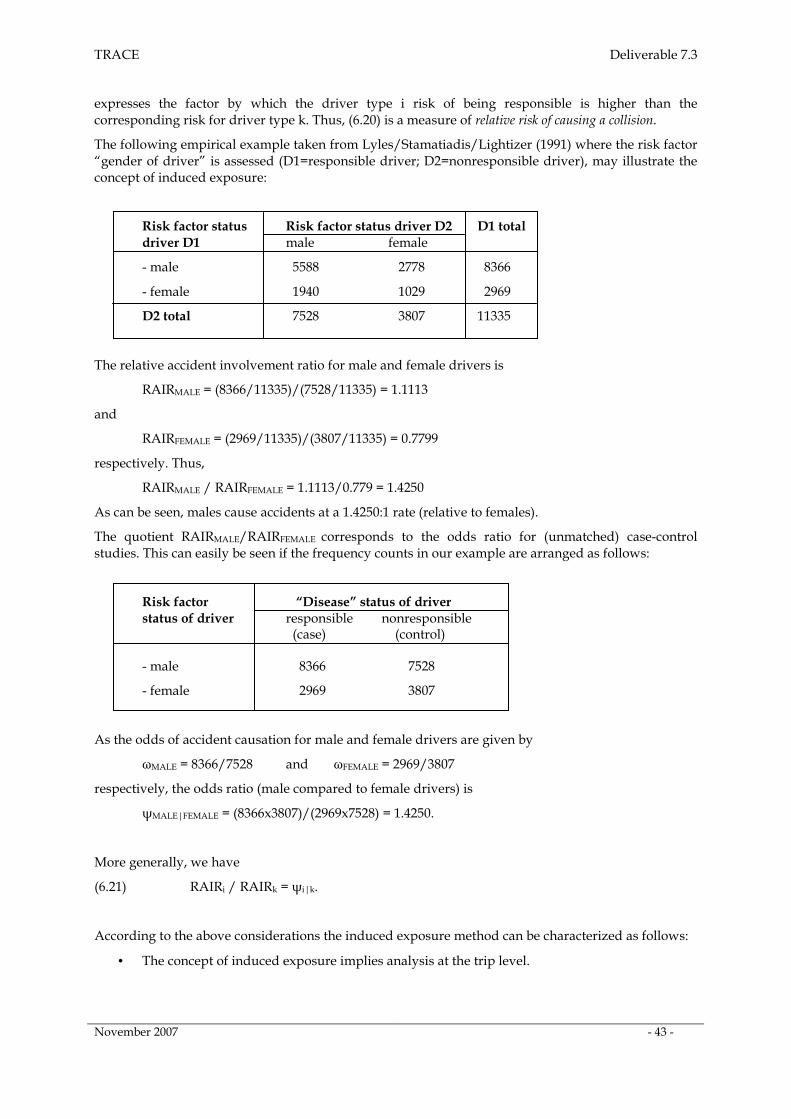
TRACE Deliverable 7.3
November 2007 - 43 -
expresses the factor by which the driver type i risk of being responsible is higher than the corresponding risk for driver type k. Thus, (6.20) is a measure of relative risk of causing a collision.
The following empirical example taken from Lyles/Stamatiadis/Lightizer (1991) where the risk factor “gender of driver” is assessed (D1=responsible driver; D2=nonresponsible driver), may illustrate the concept of induced exposure:
Risk factor status Risk factor status driver D2 D1 total driver D1 male female
- male 5588 2778 8366
- female 1940 1029 2969
D2 total 7528 3807 11335
The relative accident involvement ratio for male and female drivers is
RAIRMALE = (8366/11335)/(7528/11335) = 1.1113
and
RAIRFEMALE = (2969/11335)/(3807/11335) = 0.7799
respectively. Thus,
RAIRMALE / RAIRFEMALE = 1.1113/0.779 = 1.4250
As can be seen, males cause accidents at a 1.4250:1 rate (relative to females).
The quotient RAIRMALE/RAIRFEMALE corresponds to the odds ratio for (unmatched) case-control studies. This can easily be seen if the frequency counts in our example are arranged as follows:
Risk factor “Disease” status of driver
status of driver responsible nonresponsible (case) (control) - male 8366 7528
- female 2969 3807
As the odds of accident causation for male and female drivers are given by
ωMALE = 8366/7528 and ωFEMALE = 2969/3807
respectively, the odds ratio (male compared to female drivers) is
ψMALE|FEMALE = (8366x3807)/(2969x7528) = 1.4250.
More generally, we have
(6.21) RAIRi / RAIRk = ψi|k.
According to the above considerations the induced exposure method can be characterized as follows:
• The concept of induced exposure implies analysis at the trip level.
TRACE Deliverable 7.3
November 2007 - 44 -
• The population at risk, therefore, is a universe of driver/vehicle trips. The target event in the epidemiological sense, i.e. the particular event of interest, is “trip ends up in a two-vehicle collision caused by the trip-maker”.
• The study purpose is to identify and assess risk factors for accident causation in the above sense.
• Nonresponsible drivers involved in a two-vehicle collision are assumed to be a random sample from the population of all drivers present on the road42.
• Applying the induced exposure method to measure the relative risk of accident causation formally corresponds to a case-control design.
• Cases are drivers (driver trips) who are responsible for a two-vehicle collision. Controls are nonresponsible drivers involved in such a collision. These controls, however, are treated as if they were a random sample from the population of all non-accidental driver trips.
• The way controls are interpreted corresponds to the presumption that there are no structural differences between the sub-population of non-accidental trips and the sub-population of accidental trips of nonresponsible drivers involved in two-vehicle collisions.
• For a certain risk factor of interest, the risk measure (6.20) is a measure of relative chance of causing43 a two-vehicle collision: The odds of accident causation44 are computed for a given level i of the risk factor (type i drivers) and for a base level k of the risk factor (type k drivers). Then, an odds ratio ψi|k is calculated by relating the odds for risk factor level i to the odds for base level k.
Measuring relative risk of accident causation under the induced exposure approach by calculating the odds ratio ψi|k according to (6.21) does clearly not account for the fact that cases (responsible drivers) and controls (nonresponsible drivers) are paired as has recently been pointed out by Lardelli-Claret et al (2006). Rather, the odds ratio is calculated as if cases and controls were sampled independently. As, however, cases and controls are actually “paired by collision”, the odds ratio for paired case-control studies would be the appropriate measure of relative risk.
In our example, the paired odds ratio is to be computed as follows:
ψ*i|k = 2778/1940 = 1.4320
The results obtained without and with taking account of pairing are practically the same in this numerical example. In an investigation45 using data from the Spanish register of road crashes Lardelli-Claret et al (2006), in general, come to the conclusion that “… both classical and paired-by-collision analyses yielded similar results and can be considered equally useful alternatives for assessing the effect of driver and vehicle characteristics on the risk of causing a collision between two vehicles”. This judgement, however, might be too positive for the “classical” approach (6.20) as there are situations where a disregard of pairing leads to completely erroneous results. See, for instance, Hautzinger (2006), p. 16-19.
Lyles/Stamatiadis/Lightizer (1991) and others have identified several critical issues related to the induced exposure method. The following two issues seem to be the most crucial:
• Is there any validity in assigning relative guilt and innocence in a multi-vehicle crash?
42 More precisely, it is assumed that accidental trips of nonresponsible drivers are a random sample from the population of all trips which are either non-accidental or accidental but not made by a responsible driver. 43 Causing an accident in this context implies being involved in an accident. Thus, accident causation risk is a special type of accident involvement risk (accident involvement as guilty party). 44 “Involved as guilty party” versus “not accident-involved or innocently accident-involved” 45 In addition to risk comparisons between two groups of drivers Lardelli-Claret et al (2006) have also applied multinomial logistic regression models (classical approach) and conditional logistic regression analysis (paired-by-collision approach) to assess several risk factors simultaneously.
TRACE Deliverable 7.3
November 2007 - 45 -
• Can the innocent drivers reasonably be considered a random sample of drivers on the road?
A classical and a paired-by-collision analysis of responsible and non-responsible drivers were carried out in the TRACE project. In addition, the validity of the induced exposure concept has been checked by directly comparing the structure of non-responsible accident-involved vehicle drivers (from national traffic accident statistics) with the structure of vehicle drivers in general (from a nation-wide mobility survey).
The results can be found in Annex III.
6.3.3 Comparison of risk factor-specific and reference accident type
An alternative induced exposure approach which, for instance, can be suitable to assess the effect of a specific risk factor on accident involvement risk is built on the following basic idea: For a given risk factor to be assessed (e.g. “ESP-equipped46 vehicle”) an appropriate risk factor-specific accident type f (e.g. “skidding accident”) and a reference or neutral accident type r has to be defined47. As can be imagined, the reference accident type must be independent of the risk factor under consideration in the sense that the chance48 of involvement in such an accident can reasonably be assumed not to depend on the presence or absence of the risk factor.
As usual, the effect of the risk factor on the risk of involvement in a risk factor-specific accident can be measured by the relative risk (group with the risk factor compared to group without the risk factor). It appears that under the above assumption of independence, the relative risk of involvement in a risk factor-specific accident can be estimated by a certain odds ratio, which can be determined by using accident data only, i.e. without any information on non-accidental trips: One simply has to compute the odds of a risk factor-related accident (versus a reference accident) for those with the risk factor and those without the risk factor; the odds ratio for those with the risk factor, compared to those without, is then the desired estimate for the relative chance to be involved in a risk factor-specific accident.
In an analysis at the trip level, the population number of trips at risk may be denoted by M. Let M+
and M- be the total number of trips at risk in the subpopulation with (+) and without (-) the risk factor, respectively (M = M+ + M-). Correspondingly, the population number of accidental trips (risk factor-related accident type f) can be denoted by Y+(f) and Y-(f). Then, the (empirical) risk of involvement in a type f accident49 is given by
R+(f) = Y+(f)/M+ and R-(f) = Y-(f)/M-
for those with and those without the risk factor, respectively.
The effect of the risk factor on the risk of involvement in a type f accident can, as usual, be measured by the relative risk:
λ(f) = R+(f)/R-(f) = [Y+(f)/Y-(f)] / [M-/M+] .
Under the independence assumption (identical group-specific involvement risks as regards the reference accident type r), which can be written as
Y+(r)/M+ = Y-(r)/M-
we have M-/M+ = Y-(r)/Y+(r) and the relative risk takes on the following form:
(6.22) λ(f) = [Y+(f)/Y+(r)] / [Y-(f)/Y-(r)].
46 ESP is a protective factor rather than a risk factor in the narrow sense. 47 From an epidemiological point of view, the differentiation between two types of accidents corresponds to a
situation where the disease outcome is not a binary characteristic (disease versus no disease) but a categorical variable with several levels. In our case, “disease status” is measured at three levels (no involvement, involvement in type f accident, involvement in type r accident. For details see Woodward (1999), p. 502-506.
48 The chance of accident involvement can be measured either by the proportion of accidental trips (empirical risk, CIR) or by accident involvement density (accidental trips per km trip distance).
49 In an assessment of the protective factor “ESP”, the type r accident could be “skidding accident”.
TRACE Deliverable 7.3
November 2007 - 46 -
Thus, if the independence assumption holds, the population value λ(f) of the relative risk of involvement in a type f accident (group with the risk factor compared to group without the risk factor) can be estimated by calculating the sample value of the odds ratio appearing on the right hand side of Equation (6.22). As can be seen, this odds ratio depends only on accident involvement counts.
Obviously, in order to check the validity of the independence assumption (Y+(r)/M+ = Y-(r)/M-), empirical data both on accidental and non-accidental trips - broken down by risk factor status - are needed. If this type of information is not available, as is frequently the case, one must be aware of the threat that the sample value of the odds ratio (6.22) as the “induced exposure estimator” of the relative risk might be biased.
A slightly modified version of the above approach has been described by Hautzinger (2003). See Kreiß, Schüler and Zangmeister (2007) for a more detailed discussion of the approach in a probabilistic context. Empirical comparisons based on a distinction between risk factor-specific and reference or neutral accident types have been conducted to assess the effectiveness of active safety technologies. See Thomas (2006). A limitation of the methodology when applied to assess systems like ESP is the assumption that equipped cars (i.e. those with the risk factor) differ from those which are not equipped (i.e. those without the risk factor) only by the presence of ESP. For a critical discussion see Thomas (2006).
The approach has been investigated in detail in TRACE deliverable D7.4.
6.4 Criteria for Choosing Among Alternative Study Designs
The “true” population value of risks, odds ratios, rates and densities can only be determined by a complete census, where all units belonging to the population at risk are recorded and classified as either accidental or non-accidental. Apart from particular situations, complete accident and traffic censuses are not feasible. Therefore, samples drawn from the population at risk and/or secondary accident and exposure data are needed to estimate measures of accident involvement incidence.
The design of an empirical accident involvement study will mainly depend on two circumstances:
• possibility to collect special traffic participation and accident involvement data on the same units and
• accessibility and quality of already existing secondary traffic accident and mobility behaviour data sources.
In this chapter two possible research strategies have been described. Under the first approach, a special sample is drawn from the population at risk and information is recorded on the accident involvement status and other characteristics of each selected unit at risk. Surveys on traffic participation and accident involvement but also cohort and case-control studies of accident involvement are built on this type of sampling from the population at risk. As accident involvement is a rare event, the case-control study design has special advantages. Normally, special data collection offers the best possibility to assess the determinants of accident involvement.
Under the second approach, only already existing databases are used: Accident involvement counts from national traffic accident statistics are related to estimates of exposure quantities from representative mobility surveys (total number of trips, totals of traffic participation time or distance travelled). As compared to special data collection, the potential of studies using routine data is limited. By applying adequate statistical models, however, the accident researcher can make the most of it. If exposure data is completely missing, the induced exposure method can sometimes offer a way to estimate relative risks provided that an appropriate control group can be found among the accidental units themselves.
TRACE Deliverable 7.3
November 2007 - 47 -
7 Measuring Road User Injury Risk The statistical concepts and methods for measuring accident involvement risk as presented above can also be applied to assess the risk of being injured in a road traffic accident. It has, however, to be specified clearly what is meant by “injury risk”. In a study on injury risk of road users we may distinguish the following two different types of injury risk:
• risk of being involved and injured in an accident (unconditional road user injury risk)
• risk of being injured given accident involvement (conditional road user injury risk)
The two concepts of injury are considered in this chapter.
7.1 Unconditional Road User Injury Risk
From a descriptive point of view the unconditional road user injury risk corresponds to the proportion of trips having the following two characteristics:
• trip ends up in an accident (“accidental trip”)
• trip maker (road user) is injured in the accident50.
Thus, for investigations on unconditional road user injury risk at the trip level, the accident involvement status of the units at risk (road user trips) is to be considered as a characteristic measured at three levels51: (1) non-accidental trip, (2) accidental trip where road user remains uninjured and (3) accidental trip where road user is injured. Consequently, unconditional road user injury risk Rinj is defined as
(7.1) Rinj = Yinj/M
where the symbols Yinj and M denote the number of accidental trips where road user is injured and the total number of road user trips (accidental and non-accidental road user trips), respectively.
Similarly, the odds of road user injury is to be defined as
(7.2) Ωinj = Yinj /(M-Yinj).
With these definitions in mind, all risk measures, models and methods proposed in this report for quantifying accident involvement risk may also be applied to assess unconditional road user injury risk. As can be seen, unconditional road user injury risk may be considered simply as a specific type of accident involvement risk, namely, the risk to be involved in an accident as an injured road user.
Example
In the TRACE project the accident involvement and injury risk of car drivers has been investigated using German accident and exposure data. From national statistics (OGPAS) the number Yinj of drivers of passenger cars injured in a road traffic accident during a given calendar year is known (up to a certain dark figure, of course). The annual number M of trips made by car drivers can be estimated from a nation-wide mobility survey conducted in 2002 (MiD2002).
Both datasets are stratified with respect to
• age group and
• gender
of the car driver. Quasi-likelihood Poisson regression has been used to model the number of injured passenger car drivers, Yinj .
Details can be found in Annex I, Part C.
50 According to this definition one could also speak of road user accident involvement and injury risk. 51 See Section 2.2.3 for involvement status variables with several outcomes.
TRACE Deliverable 7.3
November 2007 - 48 -
7.2 Conditional Road User Injury Risk
Quite often, the injury risk of accident-involved road users (or, more generally, trip makers) is of interest. Crashworthiness assessment of cars where usually the vehicle’s level of passive safety is measured by conditional driver injury risk is a typical example.
Conditional road user injury risk refers to the chance of road user injury given that the road user is involved in an accident. Consequently, the population at risk is no longer the universe of all trips but rather the subset of accidental trips and, correspondingly, the disease status variable is now defined as “trip maker injured yes/no”. Clearly, the conditional road user injury risk is by far larger than the unconditional risk of road user injury.
In order to measure conditional road user injury risk at the trip level, the number Yinj of accidental trips where the road user is injured has to be related to the total number Yacc of accidental road user trips:
(7.3) Qinj|acc = Yinj /Yacc
Obviously, conditional road user injury risk assessment is possible without any information on non-accidental trips. Accident data are fully sufficient. However, as the following remark shows, standard traffic accident data as provided by national statistics or regional in-depth studies can only be used for calculating the conditional driver injury risk if all traffic accidents (i.e. injury and non-injury accidents) are registered.
Remark:
Normally, injury accidents are completely registered in national traffic accident statistics. Thus, the annual number Yinj of injured road users (more precisely: accidental trips where the road user is injured) should usually be known precisely up to a certain number of unreported cases (so-called dark figure). This, however, cannot always be assumed for the total number Yacc of accident-involved road users (accidental road user trips).
As Yacc equals Yinj plus the number of accidental trips where the road user remained uninjured, the denominator of the conditional injury risk measure Qinj requires reporting of uninjured accident-involved road users. Thus, for countries where police is reporting injury accidents only, the conditional road user injury risk Qinj cannot be calculated. The same holds for countries where accident registration is tied to the fulfilment of certain requirements referring to the type (e.g. accident under the influence of alcohol) or severity (e.g. minimum amount of material damage) of the accident.
If the target population of the accident survey under consideration (e.g. national traffic accident statistics) is only a subset of all traffic accidents one could, of course, simply disregard the group of accidents that do not belong to the target population. A typical example would be to investigate the injury risk of road users which are involved in accidents where at least one road user is injured.
Under certain circumstances, risk estimates obtained this way may be biased. Matched studies on injury risk offer powerful possibilities to overcome the problem. Cummings et al. (2003) and Hautzinger (2006) describe methods for assessing relative risks under matched study designs.
TRACE Deliverable 7.3
November 2007 - 49 -
8 Conclusions
This report shows that statistical science offers a wide variety of study designs and analysis methods suitable for the investigation of traffic accident causation. In studies on the causes of traffic accidents, accident involvement risk analysis proves to be a powerful tool. As a prerequisite for applying well established epidemiological methods for risk factor assessment in traffic accident causation research, a new conceptual framework for accident involvement risk studies has been developed in this report. Under this framework, road user trips are considered to be the basic “units at risk” and a distinction is made between accidental and non-accidental trips. Consequently, the “population at risk” consists of all trips which are exposed to the risk of ending up in a road traffic accident.
When searching for accident causes, we have to evaluate the chance that a trip which possesses a certain attribute ends up in an accident. The probability of a trip to be accidental given that a certain trip characteristic of interest has a particular value is termed the risk of accident involvement and the trip (or trip maker) characteristic under consideration is called risk factor status. The car driver characteristic “duration of licence possession” may serve as an example of a risk factor status variable: car trips made by novice drivers are more prone to be accidental compared to car trips made by drivers who got their licence years ago.
In empirical studies on the determinants of accident involvement, the population at risk will be broken down by various characteristics of the trip maker and the trip itself in order to investigate whether or not these characteristics are associated with the incidence of accident involvement. From this type of exercise one may arrive, for instance, at the descriptive finding that irrespective of driver age “novice” drivers are more prone to accident involvement than “veteran” drivers. This result, i.e. the association established between risk factor status and accident involvement status may lead to investigation of why this should be so.
The causal factors behind the descriptive finding quoted above could be attributes like “driving experience” (measured, for instance, by variables like total number of kilometres driven since acquisition of driving licence and frequency of participation in performance training programs for car drivers) and the like. Routine data on traffic participation and accident involvement will rarely contain information on such causal factors. Rather, special data collected for the study of causal factors (aetiological agents) are required. This type of data allows considering the aetiology of accident involvement.
Both descriptive and aetiological analyses are relevant in order for improvements in traffic safety to be made. Descriptive analyses give a guide to the targeting of traffic safety promotion. Aetiological analyses can tell us what to do to reduce the chance of being injured or even killed in an accident.
TRACE Deliverable 7.3
November 2007 - 50 -
References
Afifi, A.A. and S.P. Azen (1979): Statistical Analysis – A Computer Oriented Approach. 2nd Ed., New York: Academic Press
Agresti, A. (1996): Introduction to Categorical Data Analysis. New York: Wiley
Böhning, D. and S.N.A. Rampai (1997): A case-control study of non-fatal traffic accidents on hospital patients in Bangkok metropolis. Sozial- und Präventivmedizin 42: 351-356
Böhning, D. (1998): Allgemeine Epidemiologie und ihre methodischen Grundlagen (General Epidemiology and Its Methodological Foundations). München/Wien: R. Oldenbourg Verlag
Carr, B.R.A. (1969): A statistical analysis of rural Ontario accidents using induced exposure data. Accident Analysis and Prevention, 1(4): 343-357
Cochran, W.G. (1977): Sampling Techniques. 3rd Ed., New York: Wiley
Cummings, P., B. McKnight and N.S. Weiss (2003): Matched-pair cohort methods in traffic crash research. Accident Analysis and Prevention, 35: 131-141
Davies, G.A. and Y. Gao (1993): Statistical methods to support induced exposure analyses of traffic accident data. Transportation Research Record, 1401, Washington: Transportation Research Board
Evans, L. (1986): Double paired comparison – a new method to determine how occupant characteristics affect fatality risk in traffic crashes. Accident Analysis and Prevention, 18(3): 217-227
Fleiss, J.L. (1981): Statistical Methods for Rates and Proportions. 2nd Ed., New York: Wiley
Geiler, M., M. Pfeiffer and H. Hautzinger (2006): Das Unfallgeschehen im Wirtschaftsverkehr (Accidents in Commercial Traffic). Kröning: Asanger
Haight, F. (1970): A crude framework for bypassing exposure. Journal of safety research, 2(1): 26-29
Hautzinger, H., H. Dürholt, E. Hörnstein and B. Tassaux-Becker (1993): Dunkelziffer bei Unfällen mit Personenschaden (Non-reported injury accidents). Berichte der BASt, Heft M13. Bergisch Gladbach
Hautzinger, H., D. Heidemann and B. Krämer (1993): Fahrleistungserhebung 1990 - Inlandsfahrleistungen und Kfz-Unfallrisiko in der Bundesrepublik Deutschland (Mileage Survey 1990 – Total Vehicle Mileage on German Roads and Accident Involvement Risk of Motorized Vehicles in the Federal Republic of Germany). Berichte der BASt, Heft M20
Hautzinger, H. (2003): Measuring the effect of primary safety devices on accident involvement risk of passenger cars – Some methodological considerations. Working paper SARAC II project, Heilbronn: IVT
Hautzinger, H. (2006): Design and Analysis of Matched Studies in Empirical Car Safety Research. Final Report S2-246, SARAC II Project, Heilbronn: IVT
Hedayat, A.S. and B.K. Sinha (1991): Design and Inference in Finite Population Sampling. New York: Wiley
Kirk, A. and N. Stamatiadis (2001): Evaluation of the Quasi-induced Exposure. Final report for the USDOT Transportation Center. Department of Civil Engineering, University of Kentucky
Kreiß, J.-P., Schüler, L. and T. Zangmeister (2007): Statistical evaluation of the effectiveness of safety functions in vehicles based on real-world accidents. Working paper TRACE project, Braunschweig: Technical University
Langholz, B. and D.C. Thomas (1990): Nested case-control and case-cohort methods of sampling from a cohort: a critical comparison. American Journal of Epidemiology, 131: 169-176
Lardelli-Claret, P. et al (2006): Comparison between two quasi-induced exposure methods for studying risk factors for road crashes. American Journal of Epidemiology, 163: 188-195
TRACE Deliverable 7.3
November 2007 - 51 -
Lyles, R.W., P. Stamatiadis and D.R. Lightizer (1991): Quasi-induced exposure revisited. Accident Analysis and Prevention, 23(4): 275-285
McCullagh, P. and J.A. Nelder (1992): Generalized Linear Models. 2nd Ed., London: Chapman & Hall
Stamatiadis, N. and J.A. Deacon (1997): Quasi-induced exposure: Methodology and insight. Accident Analysis and Prevention, 29(1): 37-52
Thomas, P. (2006): The accident reduction effectiveness of ESC equipped cars in Great Britain. Proceedings 13th ITS World Congress and Exhibition, 8-12 October 2006. London
Thorpe, J.D. (1964): Calculating relative involvement rates in accidents without determining exposure. Australian Road Research, 2(1): 25-36
Vollset, S.E. (1993): Confidence intervals for a binomial proportion. Statistics in Medicine 12: 809-824
Woodward, M. (1999): Epidemiology – Study Design and Data Analysis. Boca Raton/London: Chapman & Hall/CRC
TRACE Deliverable 7.3
November 2007 - 52 -
Annex I
Accident Involvement and Injury Risk Analyses Combining Data from Different Sources
Part A: Distance- Related Accident Involvement Density δDistance Table A1 at the end of this section shows the number of road traffic casualties and distances travelled in millions of km for different groups of mobile persons, stratified by age, gender and their mode of traffic participation. The Casualties data have been taken from the German Road Accident Statistics from the year 2002. Trip Length data have been taken from a German Mobility Survey (MiD 2002), which has been conducted in 2002. Strata where there was insufficient Trip Length data have been excluded.
In a first step the crude risk measure for every group has been computed by dividing the number of Casualties Y by the total distance travelled by the group (Casualties per Million km). The result is depicted in Figure A2. The Accident involvement density has been plotted on a logarithmic scale, thus an increase by 1 unit refers to a 10 times higher accident involvement density.
The data has then been analysed using the statistical Computer Software R (Version 2.5.1). Poisson regression with compensation for dispersion has been used to model the data. Analysis of variance showed, that the gender effect can be neglected, giving rise to a Model2 (without gender covariate). By introducing log(MioKm) as covariate and as offset variable, respectively, it could be checked whether the coefficient of proportionality does significantly deviate from 1:
>Model1=glm(Casualties~Mode.of.Transport+AgeGroup+log(MioKm),offset=log(MioKm), family=quasipoisson, data=Km)
The results of the computation are shown in Table A3.
(Intercept) 2,861 0,912 0,003
Mode.of.Transport:Cycle.Driver 0,996 0,221 0,000 2,7
Mode.of.Transport:Moped.Driver 1,148 0,393 0,005 3,2
Mode.of.Transport:Motorcycle.Driver 1,481 0,314 0,000 4,4
Mode.of.Transport:PassengerCar.Driver 0,354 0,150 0,021 1,4
Mode.of.Transport:Pedestrian 0,300 0,234 0,203 1,4
AgeGroup[0,6) -1,040 0,333 0,003 0,4
AgeGroup[6,10) -0,573 0,308 0,067 0,6
AgeGroup[10,14) -0,470 0,253 0,068 0,6
AgeGroup[14,18) 0,285 0,224 0,207 1,3
AgeGroup[18,25) 0,395 0,160 0,016 1,5
AgeGroup[45,60) -0,470 0,128 0,000 0,6
AgeGroup[60,65) -0,973 0,247 0,000 0,4
AgeGroup[65,inf) -0,493 0,190 0,012 0,6
log(Exposure) -0,370 0,085 0,000 0,7
Parameter of Dispersion
Residual Deviance
Degrees of freedom
Model1 - distance (Exposure=MioKm) related
684
42413
65
Estimate Std.Error p-valueIncidence Density Ratio
IDR K M
Table A3: Estimates and Standard Errors for Model1, predicting the distance-related Accident Involvement Density (δKM). The last column shows the distance-related Incidence Density Ratio (IDRKM), referring to δKM of the reference group of passenger car passengers, aged 25 to 45.
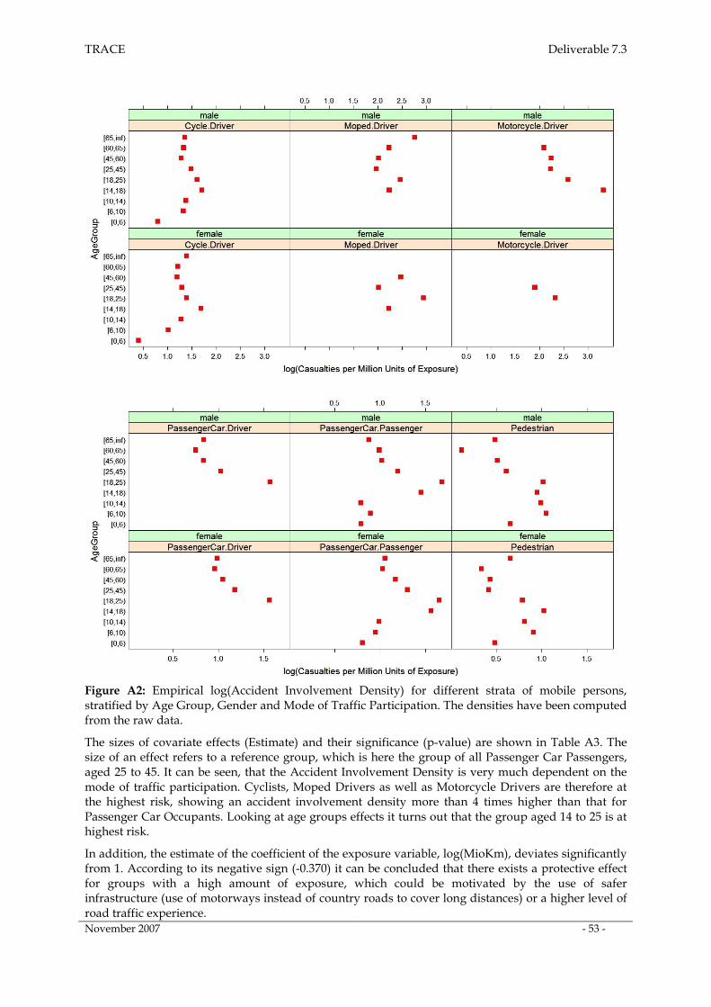
TRACE Deliverable 7.3
November 2007 - 53 -
Figure A2: Empirical log(Accident Involvement Density) for different strata of mobile persons, stratified by Age Group, Gender and Mode of Traffic Participation. The densities have been computed from the raw data.
The sizes of covariate effects (Estimate) and their significance (p-value) are shown in Table A3. The size of an effect refers to a reference group, which is here the group of all Passenger Car Passengers, aged 25 to 45. It can be seen, that the Accident Involvement Density is very much dependent on the mode of traffic participation. Cyclists, Moped Drivers as well as Motorcycle Drivers are therefore at the highest risk, showing an accident involvement density more than 4 times higher than that for Passenger Car Occupants. Looking at age groups effects it turns out that the group aged 14 to 25 is at highest risk.
In addition, the estimate of the coefficient of the exposure variable, log(MioKm), deviates significantly from 1. According to its negative sign (-0.370) it can be concluded that there exists a protective effect for groups with a high amount of exposure, which could be motivated by the use of safer infrastructure (use of motorways instead of country roads to cover long distances) or a higher level of road traffic experience.
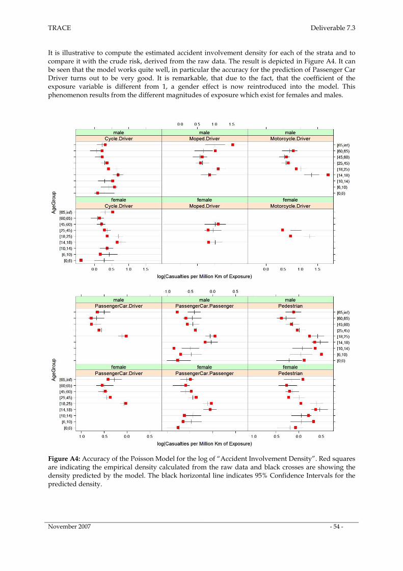
TRACE Deliverable 7.3
November 2007 - 54 -
It is illustrative to compute the estimated accident involvement density for each of the strata and to compare it with the crude risk, derived from the raw data. The result is depicted in Figure A4. It can be seen that the model works quite well, in particular the accuracy for the prediction of Passenger Car Driver turns out to be very good. It is remarkable, that due to the fact, that the coefficient of the exposure variable is different from 1, a gender effect is now reintroduced into the model. This phenomenon results from the different magnitudes of exposure which exist for females and males.
Figure A4: Accuracy of the Poisson Model for the log of “Accident Involvement Density”. Red squares are indicating the empirical density calculated from the raw data and black crosses are showing the density predicted by the model. The black horizontal line indicates 95% Confidence Intervals for the predicted density.
TRACE Deliverable 7.3
November 2007 - 55 -
Part B: Time-Related Accident Involvement Density δTime
Table B1 at the end of this section shows the number of road traffic casualties and trip duration in millions of hours for different groups of mobile persons, stratified by age, gender and their mode of traffic participation. The Casualties data have been taken from the German Road Accident Statistics from the year 2002. The total travel time, i.e. the sum of hours during which the strata have been exposed to traffic accident risk, has been taken from a German Mobility Survey (MiD2002), which has been conducted in 2002. Strata where there was insufficient data on the time in traffic have been excluded.
In a first step, the crude risk measure for every group has been computed by dividing the number of Casualties Y by the Exposure time of each group (casualties per million hours). The result is depicted in Figure B2. For comparison, the distance-related accident involvement density has been added to the plot. The Accident Involvement Density has been plotted on a logarithmic scale, thus an increase by 1 unit refers to a 10 times higher accident involvement density.
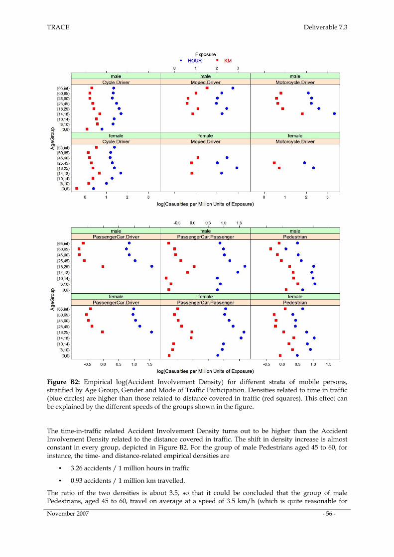
TRACE Deliverable 7.3
November 2007 - 56 -
Figure B2: Empirical log(Accident Involvement Density) for different strata of mobile persons, stratified by Age Group, Gender and Mode of Traffic Participation. Densities related to time in traffic (blue circles) are higher than those related to distance covered in traffic (red squares). This effect can be explained by the different speeds of the groups shown in the figure.
The time-in-traffic related Accident Involvement Density turns out to be higher than the Accident Involvement Density related to the distance covered in traffic. The shift in density increase is almost constant in every group, depicted in Figure B2. For the group of male Pedestrians aged 45 to 60, for instance, the time- and distance-related empirical densities are
• 3.26 accidents / 1 million hours in traffic
• 0.93 accidents / 1 million km travelled.
The ratio of the two densities is about 3.5, so that it could be concluded that the group of male Pedestrians, aged 45 to 60, travel on average at a speed of 3.5 km/h (which is quite reasonable for
TRACE Deliverable 7.3
November 2007 - 57 -
pedestrians). In an analogous manner the average speed for male Passenger Car Drivers, aged 45 to 60 is computed to be 40 km/h.
The data has again been analysed by Poisson regression with compensation for dispersion:
>Model2=glm(Casualties~Mode.of.Transport+AgeGroup+log(MioHour),offset=log(MioHour), family=quasipoisson, data=Hour)
The results are shown in Table B3.
Incidence Density Ratio
IDR TIME IDR KM
(Intercept) 4,367 0,657 0,000
Mode.of.Transport:Cycle.Driver 0,203 0,143 0,162 1,2 (2,7)
Mode.of.Transport:Moped.Driver 1,161 0,369 0,002 3,2 (3,2)
Mode.of.Transport:Motorcycle.Driver 1,773 0,325 0,000 5,9 (4,4)
Mode.of.Transport:PassengerCar.Driver 0,074 0,167 0,659 1,1 (1,4)
Mode.of.Transport:Pedestrian -1,166 0,159 0,000 0,3 (1,4)
AgeGroup[0,6) -1,083 0,320 0,001 0,3 (0,4)
AgeGroup[6,10) -0,548 0,298 0,070 0,6 (0,6)
AgeGroup[10,14) -0,443 0,245 0,074 0,6 (0,6)
AgeGroup[14,18) 0,454 0,225 0,048 1,6 (1,3)
AgeGroup[18,25) 0,621 0,173 0,001 1,9 (1,5)
AgeGroup[45,60) -0,416 0,126 0,002 0,7 (0,6)
AgeGroup[60,65) -0,854 0,243 0,001 0,4 (0,4)
AgeGroup[65,inf) -0,504 0,179 0,006 0,6 (0,6)
log(Exposure) -0,238 0,096 0,015 0,8 (0,7)
Parameter of Dispersion
Residual Deviance
Degrees of freedom
647
39013
66
Estimate Std.Error p-value
Model2 - time (Exposure=MioHour) related
Table B3: Estimates and Standard Errors for Model2, predicting the time-related Accident Involvement Density (δTIME). The last column shows the distance-related Incidence Density Ratio (IDRTIME), referring to δTIME of the reference group of passenger car passengers, aged 25 to 45. For comparison, the distance-related IDRKM has been added in brackets.
Table B3 shows the sizes of covariate effects (Estimate) and their significance (p-value). For comparison, the distance-related Accident Involvement Density Ratio (Table A3) has been added in brackets. The size of an effect refers to a reference group, which is here the group of Passenger Car Passengers, aged 25 to 45. The effect, that Cycle Drivers are more accident-prone decreases, showing that they travel at a lower speed than the reference group, which are passenger cars. Surprisingly, the density for moped drivers stays constant, although it could be assumed that they travel at a lower speed. Motorcycle Drivers remain to be at highest risk. The group of Pedestrians now shows the lowest Density, because of their low speed in traffic.
Looking at the risk factor Age Group, the effects are less obvious. The density for the group of young persons aged 14 to 25, increases. This shall be taken as an indicator that the members of this age group travel at a somewhat higher speed than the reference group. Different speeds by age group are visible in Figure B2, where the shift between time and distance related accident involvement density becomes wider with increasing age, in particular for Cyclists and Pedestrians. However, this effect exists just for the mentioned modes of traffic participation and becomes less striking when just looking for the main effect.
Again, the estimate of the coefficient of the exposure variable, log(MioHour) deviates significantly from 1, suggesting a protective effect for groups with a high amount of exposure. The reasons for that are supposed to be similar to those mentioned in Part A.
TRACE Deliverable 7.3
November 2007 - 58 -
Part C: Unconditional Road User Injury Risk ρTrip
Table C1 at the end of this section shows the number of road traffic casualties and the number of Trips (in millions) for different groups of mobile persons, stratified by age, gender and their mode of traffic participation. The Casualties data have been taken from the German Road Accident Statistics from the year 2002. Data on the number of trips has been taken from a German Mobility Survey (MID2002), which has been conducted in 2002. Strata where there was insufficient Trip data have been excluded.
Like in Parts A and B of Appendix I, quasi-likelihood Poisson regression with compensation for dispersion has been used to model the data. At this time, log(MioTrips) is a true offset variable as its coefficient does not significantly deviate from 1. Consequently, log(MioTrips) has not been included as covariate in the model:
>Model3=glm(Casualties~Mode.of.Transport+AgeGroup,offset=log(MioTrips) family=quasipoisson, data=trips)
The results of the computation are shown in Table C3.
(Intercept) 1,915 0,111 0,000
Mode.of.Transport:Cycle.Driver 0,182 0,132 0,173 1,2
Mode.of.Transport:Moped.Driver 1,479 0,229 0,000 4,4
Mode.of.Transport:Motorcycle.Driver 2,753 0,174 0,000 15,7
Mode.of.Transport:PassengerCar.Driver -0,386 0,113 0,001 0,7
Mode.of.Transport:Pedestrian -1,330 0,162 0,000 0,3
AgeGroup[0,6) -1,177 0,313 0,000 0,3
AgeGroup[6,10) -0,501 0,271 0,069 0,6
AgeGroup[10,14) -0,354 0,228 0,125 0,7
AgeGroup[14,18) 0,713 0,171 0,000 2,0
AgeGroup[18,25) 0,901 0,106 0,000 2,5
AgeGroup[45,60) -0,273 0,120 0,026 0,8
AgeGroup[60,65) -0,438 0,203 0,034 0,6
AgeGroup[65,inf) -0,286 0,156 0,071 0,8
Parameter of Dispersion
Residual Deviance
Degrees of freedom
Model3 - Trip (Number of Trips) related
690
41639
67
Estimate Std.Error p-valueRel. Acc. Involvement
Rate ρrel
Table C3: Estimates and Standard Errors for Model3, predicting the Accident Involvement Rate (ρTRIP). The last column shows the relative Accident Involvement Rate (ρrel), referring to ρTRIP of the reference group of passenger car passengers, aged 25 to 45.
The increase in accident involvement density ratio for Motorcycle Drivers is striking. The increase could be explained by the fact that motorcycles are quite often used during leisure time and, therefore, cover relatively high distances per trip, as compared to passenger cars.

TRACE Deliverable 7.3
November 2007 - 59 -
Cycle.Driver female [0,6) 145 355,9 0,4 1,9 1,0 3,7
Cycle.Driver female [10,14) 2528 1076,8 2,3 2,2 1,4 3,5
Cycle.Driver female [14,18) 2918 625,6 4,7 5,8 4,1 8,3
Cycle.Driver female [18,25) 2860 1221,3 2,3 5,1 3,9 6,5
Cycle.Driver female [25,45) 6798 3463,5 2,0 2,3 1,8 3,0
Cycle.Driver female [45,60) 4725 2898,8 1,6 1,6 1,2 2,0
Cycle.Driver female [6,10) 726 485,5 1,5 2,7 1,6 4,7
Cycle.Driver female [60,65) 2035 1437,4 1,4 1,2 0,8 1,9
Cycle.Driver female [65,inf) 4171 1212,9 3,4 2,1 1,5 2,9
Cycle.Driver male [0,6) 413 329,6 1,3 2,0 1,0 3,8
Cycle.Driver male [10,14) 5036 1465,5 3,4 2,0 1,3 3,1
Cycle.Driver male [14,18) 5035 1022,4 4,9 4,9 3,4 6,9
Cycle.Driver male [18,25) 4093 1573,9 2,6 4,6 3,6 6,0
Cycle.Driver male [25,45) 12442 5334,1 2,3 2,0 1,6 2,5
Cycle.Driver male [45,60) 6730 3965,7 1,7 1,4 1,0 1,8
Cycle.Driver male [6,10) 1957 506,6 3,9 2,7 1,5 4,6
Cycle.Driver male [60,65) 2735 1629,0 1,7 1,2 0,8 1,8
Cycle.Driver male [65,inf) 4678 2253,1 2,1 1,7 1,2 2,3
Moped.Driver female [14,18) 1284 192,7 6,7 10,5 6,6 16,6
Moped.Driver female [18,25) 641 NA NA NA NA NA
Moped.Driver female [25,45) 877 135,1 6,5 9,0 5,2 15,7
Moped.Driver female [45,60) 328 25,6 12,8 10,4 5,1 21,1
Moped.Driver male [14,18) 4698 645,3 7,3 6,7 4,0 11,2
Moped.Driver male [18,25) 1803 142,0 12,7 13,1 8,2 20,9
Moped.Driver male [25,45) 3654 929,7 3,9 4,4 2,8 6,9
Moped.Driver male [45,60) 1754 402,2 4,4 3,8 2,3 6,0
Moped.Driver male [60,65) 565 54,0 10,5 4,8 2,6 8,8
Moped.Driver male [65,inf) 836 24,5 34,2 10,3 5,4 19,9
Motorcycle.Driver female [18,25) 706 136,5 5,2 18,5 12,7 27,1
Motorcycle.Driver female [25,45) 1716 570,9 3,0 7,4 5,1 10,6
Motorcycle.Driver male [14,18) 4628 71,9 64,4 21,0 12,8 34,7
Motorcycle.Driver male [18,25) 5036 664,7 7,6 10,3 7,5 14,3
Motorcycle.Driver male [25,45) 15039 3370,0 4,5 3,8 2,8 5,2
Motorcycle.Driver male [45,60) 5094 1307,4 3,9 3,4 2,4 4,8
Motorcycle.Driver male [60,65) 813 130,3 6,2 4,8 2,9 8,0
PassengerCar.Driver female [18,25) 24965 26438,0 0,9 0,9 0,7 1,0
PassengerCar.Driver female [25,45) 42254 97768,9 0,4 0,4 0,3 0,4
PassengerCar.Driver female [45,60) 15062 44854,9 0,3 0,3 0,2 0,4
PassengerCar.Driver female [60,65) 2560 8887,4 0,3 0,3 0,2 0,5
PassengerCar.Driver female [65,inf) 3497 9015,1 0,4 0,5 0,4 0,8
PassengerCar.Driver male [18,25) 32626 33767,6 1,0 0,8 0,7 0,9
PassengerCar.Driver male [25,45) 47338 194436,2 0,2 0,3 0,2 0,3
PassengerCar.Driver male [45,60) 18759 111660,1 0,2 0,2 0,2 0,3
PassengerCar.Driver male [60,65) 4602 27881,3 0,2 0,2 0,1 0,3
PassengerCar.Driver male [65,inf) 7910 35099,9 0,2 0,3 0,2 0,4
PassengerCar.Passenger female [0,6) 2403 13932,4 0,2 0,2 0,1 0,3
PassengerCar.Passenger female [10,14) 2474 10369,3 0,2 0,4 0,2 0,6
PassengerCar.Passenger female [14,18) 6606 7497,8 0,9 0,9 0,6 1,2
PassengerCar.Passenger female [18,25) 12546 13472,2 0,9 0,8 0,6 1,0
PassengerCar.Passenger female [25,45) 15518 35920,7 0,4 0,4 0,3 0,5
PassengerCar.Passenger female [45,60) 8702 25747,5 0,3 0,3 0,2 0,3
PassengerCar.Passenger female [6,10) 2025 9037,4 0,2 0,3 0,2 0,6
PassengerCar.Passenger female [60,65) 3165 12429,0 0,3 0,2 0,1 0,3
PassengerCar.Passenger female [65,inf) 6797 20918,5 0,3 0,3 0,2 0,4
PassengerCar.Passenger male [0,6) 2427 14311,7 0,2 0,2 0,1 0,3
PassengerCar.Passenger male [10,14) 1931 13754,3 0,1 0,3 0,2 0,5
PassengerCar.Passenger male [14,18) 4253 6274,0 0,7 0,9 0,7 1,3
PassengerCar.Passenger male [18,25) 10941 9771,4 1,1 0,9 0,7 1,1
PassengerCar.Passenger male [25,45) 9346 22681,5 0,4 0,4 0,3 0,5
PassengerCar.Passenger male [45,60) 2718 9811,2 0,3 0,4 0,3 0,5
PassengerCar.Passenger male [6,10) 1857 9407,1 0,2 0,3 0,2 0,6
AID.KM.
LOWER.CI
AID.KM.
UPPER.CI
Exposure.
MioKm
AID.
KM
AID.KM.
ESTIMATEDMode.of.Transport Gender AgeGroup Casualties
Table A1: Road traffic casualties and kilometres travelled

TRACE Deliverable 7.3
November 2007 - 60 -
Cycle.Driver female [0,6) 145 57,3 2,5 12,5 6,6 23,4
Cycle.Driver female [10,14) 2528 133,2 19,0 19,3 12,6 29,7
Cycle.Driver female [14,18) 2918 59,9 48,7 57,4 40,7 80,9
Cycle.Driver female [18,25) 2860 117,2 24,4 57,9 45,2 74,1
Cycle.Driver female [25,45) 6798 344,9 19,7 24,0 19,0 30,4
Cycle.Driver female [45,60) 4725 301,9 15,7 16,4 12,5 21,4
Cycle.Driver female [6,10) 726 70,4 10,3 20,3 12,0 34,2
Cycle.Driver female [60,65) 2035 124,8 16,3 13,0 8,6 19,7
Cycle.Driver female [65,inf) 4171 169,7 24,6 17,2 12,5 23,7
Cycle.Driver male [0,6) 413 65,7 6,3 12,1 6,5 22,5
Cycle.Driver male [10,14) 5036 211,0 23,9 17,3 11,2 26,8
Cycle.Driver male [14,18) 5035 100,0 50,3 50,8 36,3 71,0
Cycle.Driver male [18,25) 4093 100,7 40,6 60,0 46,9 76,7
Cycle.Driver male [25,45) 12442 407,3 30,5 23,1 18,3 29,1
Cycle.Driver male [45,60) 6730 348,6 19,3 15,8 12,1 20,7
Cycle.Driver male [6,10) 1957 93,1 21,0 19,0 11,3 31,9
Cycle.Driver male [60,65) 2735 127,4 21,5 13,0 8,6 19,6
Cycle.Driver male [65,inf) 4678 207,7 22,5 16,4 11,8 22,7
Moped.Driver female [14,18) 1284 7,7 167,5 244,2 157,6 378,4
Moped.Driver female [18,25) 641 0,7 878,1 505,2 262,1 973,9
Moped.Driver female [25,45) 877 8,4 104,5 151,8 90,2 255,3
Moped.Driver female [45,60) 328 1,1 299,5 162,5 77,1 342,7
Moped.Driver male [14,18) 4698 27,0 173,9 180,9 110,5 296,3
Moped.Driver male [18,25) 1803 6,2 290,6 303,6 194,2 474,8
Moped.Driver male [25,45) 3654 38,7 94,4 105,5 69,0 161,5
Moped.Driver male [45,60) 1754 16,8 104,5 84,9 53,6 134,3
Moped.Driver male [60,65) 565 3,3 172,0 80,8 45,0 145,1
Moped.Driver male [65,inf) 836 1,5 572,6 139,0 71,7 269,5
Motorcycle.Driver female [18,25) 706 3,3 214,9 651,3 440,0 964,1
Motorcycle.Driver female [25,45) 1716 21,2 81,1 224,6 161,6 312,1
Motorcycle.Driver male [14,18) 4628 2,2 2113,2 606,7 366,8 1003,5
Motorcycle.Driver male [18,25) 5036 12,8 394,2 471,5 344,1 646,0
Motorcycle.Driver male [25,45) 15039 87,2 172,4 160,3 117,6 218,6
Motorcycle.Driver male [45,60) 5094 28,8 176,7 137,6 98,2 193,0
Motorcycle.Driver male [60,65) 813 6,6 123,7 126,3 78,7 202,8
PassengerCar.Driver female [18,25) 24965 688,0 36,3 33,4 27,8 40,0
PassengerCar.Driver female [25,45) 42254 2810,1 15,0 12,8 11,0 14,9
PassengerCar.Driver female [45,60) 15062 1353,8 11,1 10,1 8,1 12,6
PassengerCar.Driver female [60,65) 2560 281,1 9,1 9,4 6,2 14,4
PassengerCar.Driver female [65,inf) 3497 361,7 9,7 12,6 8,7 18,3
PassengerCar.Driver male [18,25) 32626 890,6 36,6 31,4 26,2 37,6
PassengerCar.Driver male [25,45) 47338 4471,6 10,6 11,5 9,8 13,4
PassengerCar.Driver male [45,60) 18759 2744,4 6,8 8,5 6,9 10,6
PassengerCar.Driver male [60,65) 4602 817,6 5,6 7,3 5,0 10,7
PassengerCar.Driver male [65,inf) 7910 1149,8 6,9 9,6 7,2 12,8
PassengerCar.Passenger female [0,6) 2403 375,6 6,4 6,5 3,6 11,7
PassengerCar.Passenger female [10,14) 2474 254,4 9,7 13,5 8,9 20,7
PassengerCar.Passenger female [14,18) 6606 181,8 36,3 36,0 26,2 49,5
PassengerCar.Passenger female [18,25) 12546 281,4 44,6 38,3 30,4 48,3
PassengerCar.Passenger female [25,45) 15518 777,5 20,0 16,2 13,1 20,0
PassengerCar.Passenger female [45,60) 8702 588,0 14,8 11,4 8,8 14,7
PassengerCar.Passenger female [6,10) 2025 227,4 8,9 12,5 7,6 20,7
PassengerCar.Passenger female [60,65) 3165 295,3 10,7 8,7 5,8 13,1
PassengerCar.Passenger female [65,inf) 6797 599,3 11,3 10,4 7,5 14,4
PassengerCar.Passenger male [0,6) 2427 391,3 6,2 6,4 3,6 11,6
PassengerCar.Passenger male [10,14) 1931 313,5 6,2 12,9 8,4 19,7
PassengerCar.Passenger male [14,18) 4253 150,7 28,2 37,6 27,3 51,8
PassengerCar.Passenger male [18,25) 10941 228,5 47,9 40,3 32,2 50,5
PassengerCar.Passenger male [25,45) 9346 599,0 15,6 17,2 13,8 21,5
PassengerCar.Passenger male [45,60) 2718 259,2 10,5 13,9 10,4 18,5
PassengerCar.Passenger male [6,10) 1857 237,6 7,8 12,4 7,5 20,5
AID.TIME.
ESTIMATED
AID.TIME.
LOWER.CI
AID.TIME.
UPPER.CIMode.of.Transport Gender AgeGroup Casualties
Exposure.
MioHour
AID.
TIME
Table B1: Road traffic casualties and time spent travelled

TRACE Deliverable 7.3
November 2007 - 61 -
Cycle.Driver female [0,6) 145 145,6 1,0 2,5 1,3 4,7
Cycle.Driver female [10,14) 2528 436,2 5,8 5,7 3,7 8,9
Cycle.Driver female [14,18) 2918 209,5 13,9 16,6 11,8 23,4
Cycle.Driver female [18,25) 2860 279,6 10,2 20,1 15,5 25,9
Cycle.Driver female [25,45) 6798 1194,3 5,7 8,1 6,4 10,3
Cycle.Driver female [45,60) 4725 872,0 5,4 6,2 4,7 8,2
Cycle.Driver female [6,10) 726 190,9 3,8 4,9 2,9 8,5
Cycle.Driver female [60,65) 2035 364,6 5,6 5,3 3,5 8,0
Cycle.Driver female [65,inf) 4171 562,8 7,4 6,1 4,4 8,5
Cycle.Driver male [0,6) 413 154,8 2,7 2,5 1,3 4,7
Cycle.Driver male [10,14) 5036 609,6 8,3 5,7 3,7 8,9
Cycle.Driver male [14,18) 5035 361,7 13,9 16,6 11,8 23,4
Cycle.Driver male [18,25) 4093 353,0 11,6 20,1 15,5 25,9
Cycle.Driver male [25,45) 12442 1080,0 11,5 8,1 6,4 10,3
Cycle.Driver male [45,60) 6730 794,6 8,5 6,2 4,7 8,2
Cycle.Driver male [6,10) 1957 221,9 8,8 4,9 2,9 8,5
Cycle.Driver male [60,65) 2735 323,4 8,5 5,3 3,5 8,0
Cycle.Driver male [65,inf) 4678 514,3 9,1 6,1 4,4 8,5
Moped.Driver female [14,18) 1284 24,8 51,7 60,8 38,6 95,9
Moped.Driver female [18,25) 641 6,6 97,6 73,4 46,6 115,5
Moped.Driver female [25,45) 877 69,0 12,7 29,8 19,3 46,1
Moped.Driver female [45,60) 328 5,1 64,2 22,7 14,2 36,2
Moped.Driver male [14,18) 4698 79,6 59,0 60,8 38,6 95,9
Moped.Driver male [18,25) 1803 21,5 83,7 73,4 46,6 115,5
Moped.Driver male [25,45) 3654 146,0 25,0 29,8 19,3 46,1
Moped.Driver male [45,60) 1754 47,5 37,0 22,7 14,2 36,2
Moped.Driver male [60,65) 565 12,0 46,9 19,2 10,9 34,0
Moped.Driver male [65,inf) 836 8,8 95,4 22,4 13,4 37,3
Motorcycle.Driver female [18,25) 706 7,3 96,7 262,3 191,3 359,5
Motorcycle.Driver female [25,45) 1716 22,6 75,8 106,5 78,6 144,3
Motorcycle.Driver male [14,18) 4628 7,3 634,0 217,4 142,1 332,4
Motorcycle.Driver male [18,25) 5036 37,2 135,3 262,3 191,3 359,5
Motorcycle.Driver male [25,45) 15039 124,8 120,5 106,5 78,6 144,3
Motorcycle.Driver male [45,60) 5094 44,2 115,3 81,0 57,1 115,1
Motorcycle.Driver male [60,65) 813 6,9 117,2 68,7 42,4 111,4
PassengerCar.Driver female [18,25) 24965 1914,4 13,0 11,4 9,4 13,7
PassengerCar.Driver female [25,45) 42254 9209,0 4,6 4,6 4,0 5,4
PassengerCar.Driver female [45,60) 15062 4270,9 3,5 3,5 2,8 4,3
PassengerCar.Driver female [60,65) 2560 881,1 2,9 3,0 2,0 4,4
PassengerCar.Driver female [65,inf) 3497 1100,1 3,2 3,5 2,6 4,7
PassengerCar.Driver male [18,25) 32626 2385,3 13,7 11,4 9,4 13,7
PassengerCar.Driver male [25,45) 47338 10460,9 4,5 4,6 4,0 5,4
PassengerCar.Driver male [45,60) 18759 6624,4 2,8 3,5 2,8 4,3
PassengerCar.Driver male [60,65) 4602 1981,2 2,3 3,0 2,0 4,4
PassengerCar.Driver male [65,inf) 7910 2717,4 2,9 3,5 2,6 4,7
PassengerCar.Passenger female [0,6) 2403 1448,3 1,7 2,1 1,2 3,8
PassengerCar.Passenger female [10,14) 2474 820,2 3,0 4,8 3,1 7,4
PassengerCar.Passenger female [14,18) 6606 493,1 13,4 13,9 10,0 19,3
PassengerCar.Passenger female [18,25) 12546 642,0 19,5 16,7 13,2 21,2
PassengerCar.Passenger female [25,45) 15518 1842,9 8,4 6,8 5,4 8,5
PassengerCar.Passenger female [45,60) 8702 1384,1 6,3 5,2 4,0 6,7
PassengerCar.Passenger female [6,10) 2025 847,2 2,4 4,1 2,5 6,9
PassengerCar.Passenger female [60,65) 3165 700,8 4,5 4,4 2,9 6,6
PassengerCar.Passenger female [65,inf) 6797 1542,5 4,4 5,1 3,7 7,0
PassengerCar.Passenger male [0,6) 2427 1489,2 1,6 2,1 1,2 3,8
PassengerCar.Passenger male [10,14) 1931 828,2 2,3 4,8 3,1 7,4
PassengerCar.Passenger male [14,18) 4253 346,0 12,3 13,9 10,0 19,3
PassengerCar.Passenger male [18,25) 10941 462,8 23,6 16,7 13,2 21,2
PassengerCar.Passenger male [25,45) 9346 1195,0 7,8 6,8 5,4 8,5
PassengerCar.Passenger male [45,60) 2718 555,2 4,9 5,2 4,0 6,7
PassengerCar.Passenger male [6,10) 1857 887,3 2,1 4,1 2,5 6,9
AIR.
UPPER.CI
Exposure.
MioTripsAIR
AIR.
ESTIMATED
AIR.
LOWER.CIMode.of.Transport Gender AgeGroup Casualties
Table C1: Road traffic casualties and number of trips
TRACE Deliverable 7.3
November 2007 - 62 -
Annex II
Study Designs Based on Sampling from the Population at Risk
Part A: Survey on Accident Involvement and Injury Incidence
1. Description of the Survey
In the context of a research project on non-reported or non-recorded traffic accidents (“dark figure of official traffic accident statistics”), a regional survey among school children and students aged 6 to 24 years was conducted in southern Germany where, among other items, individuals were asked whether or not they were involved in an accident during a certain reporting period (Hautzinger, Dürholt, Hörnstein & Tassaux-Becker, 1993). This survey may serve as a practical example of an accident involvement incidence sample survey providing the empirical database for a traffic accident involvement risk study at the person-year level.
As a specific calendar year was the reporting period of the survey, the population at risk consists of all person-years of persons aged 6 to 24 years who were attending a school in the study region at the time of the survey. According to the files of the school authorities, in total 57616 school children and students visited a school located in the study area (the number of schools was 148). Thus, the total number of person-years at risk, i.e. the size of the population at risk was N= 57616.
Originally, it was planned to collect traffic accident involvement information on all N units from this population. Due to nonresponse, however, such information was actually obtained only for a sample of n=36924 units (person-years). In order to correct for nonresponse, this sample was weighted by type of community (urban, rural), type of school (6 categories) and year/grade of student (13 categories).
2. Sample measures of chance of accident involvement
Data preparation and analysis led to the result that nA=1109 sample units may be classified as “accidental” whereas the remaining n-nA=35815 units proved to be “non-accidental”. No multiple accident involvement of the same individual during the study period had been reported by the respondents. According to the above results, the observed sample risk of accident involvement is
(1) r = nA /n = 1109/36924 = 0.03003 (=3.0%)
i.e. on average, 3 out of 100 individuals were involved in a traffic accident during the study year.
The chance of accident involvement may also be measured by the odds of accident involvement:
(1*) ω = nA /(n - nA) = 1109/35815 = 0.03096.
This measure tells us that in the sample drawn from the population at risk non-accidental person-years are roughly 32 times more frequent than accidental person-years (1/ω = 32.3).
3. Involvement risk estimation for an actual finite population at risk
If we interpret our data as a random sample of size n drawn without replacement from the above actual finite population of N person-years at risk, the sample risk r = 0.030 may be used as an estimate of the population risk R = NA/N (population proportion of accidental person-years). Under the above assumption, the estimate of var(r) is given by
(2) s2(r) = (1 – f)r(1-r)/(n – 1)
where f=n/N is the sampling fraction and (1 – f) is the finite population correction factor. In our practical example, the standard error of r is estimated at
(3) s(r) = √[(1 – 0.641) × 0.030 × 0.970 /35814] = 0.00054.
TRACE Deliverable 7.3
November 2007 - 63 -
Thus, the approximate 95 percent two-sided confidence interval for R is given by
(4) r ± 1.96 × 0.00054 or r ± 0.00106.
This means that we can be confident that the interval (0.029, 0.031) covers the unknown true population risk R. As both the sample size n and the sampling fraction f are large, this interval is very narrow.
It should be noted that formula (2) refers to the case where sample size is fixed in advance by the researcher. In a situation where nonresponse occurs, the sample size n is random, leading to a more complex variance estimate. This problem, however, is neglected here. Needless to say, the confidence interval is only valid if nonresponse bias has been removed by the above mentioned weighting procedure.
4. Involvement risk estimation for a hypothetical population at risk
If we assume our data set to be a simple random sample drawn from the hypothetical population of all person-years at risk which are “comparable” to the person-years in our study region and study period, the finite population correction factor must be omitted since this hypothetical population is conceivably infinite. Accordingly, the estimate of the standard error of r is now given by (see Section 4.2.1)
(5) s(r) = √[0.030 × 0.970 /35814] = 0.00090.
For the purpose of making confidence statements about the involvement risk R0 referring to this hypothetical population at risk, the approximate 95 percent two-sided confidence interval is to be calculated as follows:
(6) r ± 1.96 × 0.00090 or r ± 0.00177.
As can be seen, the confidence interval for R0 ranges from 2.8% to 3.2%. Due to the large sample size this interval in absolute terms is only slightly broader than the confidence interval for R.
Remark: The population of a risk study is not always easily definable and can sometimes be either actual or hypothetical. Therefore, the researcher is urged to give careful thought to this question so as not to overgeneralise the conclusions of his or her research (Afifi & Azen, 1979, pp. 358-359).
5. Differentiating between several types of accident involvement
As described in Section 2.2.2, accident involvement status may be measured at several levels. If so, involvement risk refers to specific types or variants of road traffic accident involvement. The type or variant of involvement may be defined either by characteristics which can be observed at all units at risk (e.g. “involvement as user of a specific travel mode”) or by characteristics which can be attributed only to accidental units (e.g. “involvement with a specific severity of accidental injury”).
Grouping characteristics observable at all units at risk
In this situation, the complete population at risk is to be grouped by the characteristic under consideration. For risk assessment at the person-year level, the characteristics “age group of person” and “usage of a specific travel mode i during the study year (yes/no)” could serve as examples.
As the above described survey focussed on topics related to the dark figure of official traffic accident statistics, respondents had not been asked whether or not they participated in traffic during the study year using a specific travel mode. Rather, only accident-involved individuals had to report the travel mode for the trip that ended up in an accident. Thus, for instance, no “risk of being involved in an accident as rider of a bicycle” can be calculated here since the total number of units at risk (number of individuals that have participated in traffic as cyclists) is not known. Of course, for a travel mode like
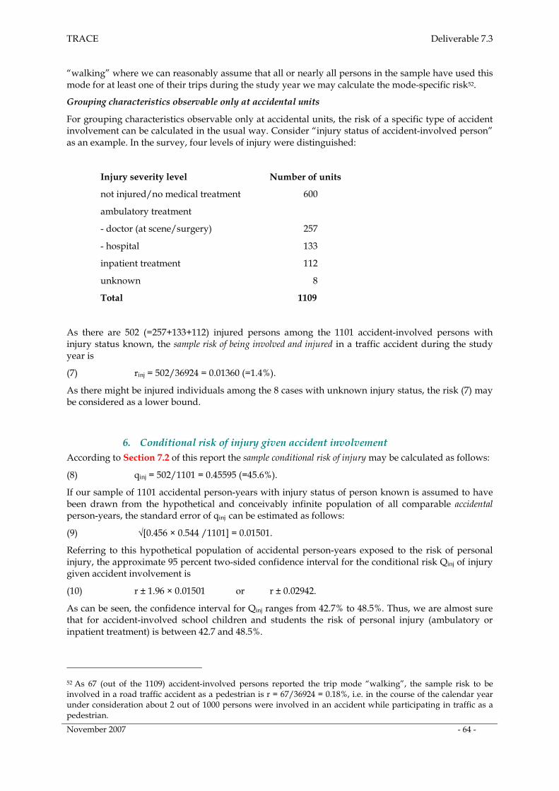
TRACE Deliverable 7.3
November 2007 - 64 -
“walking” where we can reasonably assume that all or nearly all persons in the sample have used this mode for at least one of their trips during the study year we may calculate the mode-specific risk52.
Grouping characteristics observable only at accidental units
For grouping characteristics observable only at accidental units, the risk of a specific type of accident involvement can be calculated in the usual way. Consider “injury status of accident-involved person” as an example. In the survey, four levels of injury were distinguished:
Injury severity level Number of units
not injured/no medical treatment 600
ambulatory treatment
- doctor (at scene/surgery) 257
- hospital 133
inpatient treatment 112
unknown 8
Total 1109
As there are 502 (=257+133+112) injured persons among the 1101 accident-involved persons with injury status known, the sample risk of being involved and injured in a traffic accident during the study year is
(7) rinj = 502/36924 = 0.01360 (=1.4%).
As there might be injured individuals among the 8 cases with unknown injury status, the risk (7) may be considered as a lower bound.
6. Conditional risk of injury given accident involvement
According to Section 7.2 of this report the sample conditional risk of injury may be calculated as follows:
(8) qinj = 502/1101 = 0.45595 (=45.6%).
If our sample of 1101 accidental person-years with injury status of person known is assumed to have been drawn from the hypothetical and conceivably infinite population of all comparable accidental person-years, the standard error of qinj can be estimated as follows:
(9) √[0.456 × 0.544 /1101] = 0.01501.
Referring to this hypothetical population of accidental person-years exposed to the risk of personal injury, the approximate 95 percent two-sided confidence interval for the conditional risk Qinj of injury given accident involvement is
(10) r ± 1.96 × 0.01501 or r ± 0.02942.
As can be seen, the confidence interval for Qinj ranges from 42.7% to 48.5%. Thus, we are almost sure that for accident-involved school children and students the risk of personal injury (ambulatory or inpatient treatment) is between 42.7 and 48.5%.
52 As 67 (out of the 1109) accident-involved persons reported the trip mode “walking”, the sample risk to be involved in a road traffic accident as a pedestrian is r = 67/36924 = 0.18%, i.e. in the course of the calendar year under consideration about 2 out of 1000 persons were involved in an accident while participating in traffic as a pedestrian.
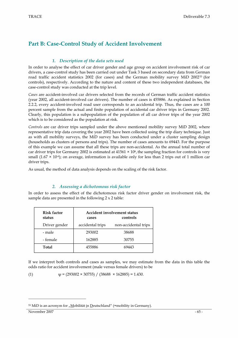
TRACE Deliverable 7.3
November 2007 - 65 -
Part B: Case-Control Study of Accident Involvement
1. Description of the data sets used
In order to analyse the effect of car driver gender and age group on accident involvement risk of car drivers, a case-control study has been carried out under Task 3 based on secondary data from German road traffic accident statistics 2002 (for cases) and the German mobility survey MiD 200253 (for controls), respectively. According to the nature and content of these two independent databases, the case-control study was conducted at the trip level.
Cases are accident-involved car drivers selected from the records of German traffic accident statistics (year 2002, all accident-involved car drivers). The number of cases is 455886. As explained in Section 2.2.2, every accident-involved road user corresponds to an accidental trip. Thus, the cases are a 100 percent sample from the actual and finite population of accidental car driver trips in Germany 2002. Clearly, this population is a subpopulation of the population of all car driver trips of the year 2002 which is to be considered as the population at risk.
Controls are car driver trips sampled under the above mentioned mobility survey MiD 2002, where representative trip data covering the year 2002 have been collected using the trip diary technique. Just as with all mobility surveys, the MiD survey has been conducted under a cluster sampling design (households as clusters of persons and trips). The number of cases amounts to 69443. For the purpose of this example we can assume that all these trips are non-accidental. As the annual total number of car driver trips for Germany 2002 is estimated at 41561 × 106, the sampling fraction for controls is very small (1.67 × 10⁻⁶); on average, information is available only for less than 2 trips out of 1 million car driver trips.
As usual, the method of data analysis depends on the scaling of the risk factor.
2. Assessing a dichotomous risk factor
In order to assess the effect of the dichotomous risk factor driver gender on involvement risk, the sample data are presented in the following 2 x 2 table:
Risk factor Accident involvement status status cases controls
Driver gender accidental trips non-accidental trips
- male 293002 38688
- female 162885 30755
Total 455886 69443
If we interpret both controls and cases as samples, we may estimate from the data in this table the odds ratio for accident involvement (male versus female drivers) to be
(1) ψ = (293002 × 30755) / (38688 × 162885) = 1.430.
53 MiD is an acronym for „Mobilität in Deutschland“ (=mobility in Germany).
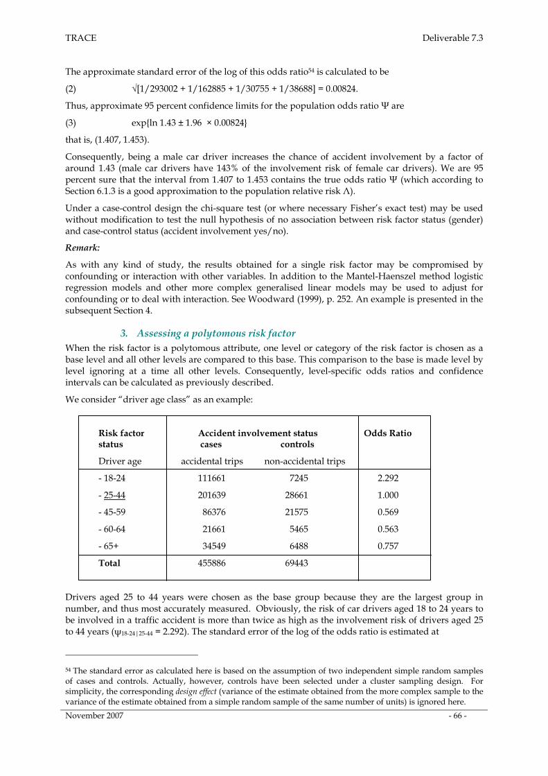
TRACE Deliverable 7.3
November 2007 - 66 -
The approximate standard error of the log of this odds ratio54 is calculated to be
(2) √[1/293002 + 1/162885 + 1/30755 + 1/38688] = 0.00824.
Thus, approximate 95 percent confidence limits for the population odds ratio Ψ are
(3) expln 1.43 ± 1.96 × 0.00824
that is, (1.407, 1.453).
Consequently, being a male car driver increases the chance of accident involvement by a factor of around 1.43 (male car drivers have 143% of the involvement risk of female car drivers). We are 95 percent sure that the interval from 1.407 to 1.453 contains the true odds ratio Ψ (which according to Section 6.1.3 is a good approximation to the population relative risk Λ).
Under a case-control design the chi-square test (or where necessary Fisher’s exact test) may be used without modification to test the null hypothesis of no association between risk factor status (gender) and case-control status (accident involvement yes/no).
Remark:
As with any kind of study, the results obtained for a single risk factor may be compromised by confounding or interaction with other variables. In addition to the Mantel-Haenszel method logistic regression models and other more complex generalised linear models may be used to adjust for confounding or to deal with interaction. See Woodward (1999), p. 252. An example is presented in the subsequent Section 4.
3. Assessing a polytomous risk factor
When the risk factor is a polytomous attribute, one level or category of the risk factor is chosen as a base level and all other levels are compared to this base. This comparison to the base is made level by level ignoring at a time all other levels. Consequently, level-specific odds ratios and confidence intervals can be calculated as previously described.
We consider “driver age class” as an example:
Risk factor Accident involvement status Odds Ratio status cases controls
Driver age accidental trips non-accidental trips
- 18-24 111661 7245 2.292
- 25-44 201639 28661 1.000
- 45-59 86376 21575 0.569
- 60-64 21661 5465 0.563
- 65+ 34549 6488 0.757
Total 455886 69443
Drivers aged 25 to 44 years were chosen as the base group because they are the largest group in number, and thus most accurately measured. Obviously, the risk of car drivers aged 18 to 24 years to be involved in a traffic accident is more than twice as high as the involvement risk of drivers aged 25 to 44 years (ψ18-24|25-44 = 2.292). The standard error of the log of the odds ratio is estimated at
54 The standard error as calculated here is based on the assumption of two independent simple random samples of cases and controls. Actually, however, controls have been selected under a cluster sampling design. For simplicity, the corresponding design effect (variance of the estimate obtained from the more complex sample to the variance of the estimate obtained from a simple random sample of the same number of units) is ignored here.
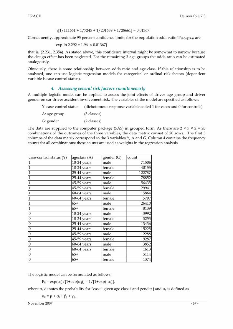
TRACE Deliverable 7.3
November 2007 - 67 -
√[1/111661 + 1/7245 + 1/201639 + 1/28661] = 0.01367.
Consequently, approximate 95 percent confidence limits for the population odds ratio Ψ18-24|25-44 are
expln 2.292 ± 1.96 × 0.01367
that is, (2.231, 2.354). As stated above, this confidence interval might be somewhat to narrow because the design effect has been neglected. For the remaining 3 age groups the odds ratio can be estimated analogously.
Obviously, there is some relationship between odds ratio and age class. If this relationship is to be analysed, one can use logistic regression models for categorical or ordinal risk factors (dependent variable is case-control status).
4. Assessing several risk factors simultaneously
A multiple logistic model can be applied to assess the joint effects of driver age group and driver gender on car driver accident involvement risk. The variables of the model are specified as follows:
Y: case-control status (dichotomous response variable coded 1 for cases and 0 for controls)
A: age group (5 classes)
G: gender (2 classes)
The data are supplied to the computer package (SAS) in grouped form. As there are 2 × 5 × 2 = 20 combinations of the outcomes of the three variables, the data matrix consist of 20 rows. The first 3 columns of the data matrix correspond to the 3 variables Y, A and G. Column 4 contains the frequency counts for all combinations; these counts are used as weights in the regression analysis.
case-control status (Y) ageclass (A) gender (G) count1 18-24 years male 715061 18-24 years female 401551 25-44 years male 1227871 25-44 years female 788521 45-59 years male 564351 45-59 years female 299411 60-64 years male 158641 60-64 years female 57971 65+ male 264101 65+ female 81390 18-24 years male 39920 18-24 years female 32530 25-44 years male 134360 25-44 years female 152250 45-59 years male 122880 45-59 years female 92870 60-64 years male 38520 60-64 years female 16130 65+ male 51140 65+ female 1374
The logistic model can be formulated as follows:
Pij = exp(uij)/[1+exp(uij)] = 1/[1+exp(-uij)].
where pij denotes the probability for “case” given age class i and gender j and uij is defined as
uij = µ + αi + βj + γij.
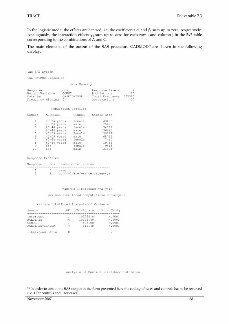
TRACE Deliverable 7.3
November 2007 - 68 -
In the logistic model the effects are centred, i.e. the coefficients αi and βj sum up to zero, respectively. Analogously, the interaction effects γij sum up to zero for each row i and column j in the 5x2 table corresponding to the combinations of A and G.
The main elements of the output of the SAS procedure CADMOD55 are shown in the following display:
The SAS System The CATMOD Procedure Data Summary Response ccs Response Levels 2 Weight Variable COUNT Populations 10 Data Set CASECONTROL Total Frequency 525320 Frequency Missing 0 Observations 20 Population Profiles Sample AGECLASS GENDER Sample Size ---------------------------------------------- 1 18-24 years female 43408 2 18-24 years male 75498 3 25-44 years female 94077 4 25-44 years male 136223 5 45-59 years female 39228 6 45-59 years male 68723 7 60-64 years female 7410 8 60-64 years male 19716 9 65+ female 9513 10 65+ male 31524 Response Profiles Response ccs case-control status --------------------------------------------- 1 0 case 2 1 control (reference category) Maximum Likelihood Analysis Maximum likelihood computations converged. Maximum Likelihood Analysis of Variance Source DF Chi-Square Pr > ChiSq -------------------------------------------------- Intercept 1 102090.0 <.0001 AGECLASS 4 10004.60 <.0001 GENDER 1 523.00 <.0001 AGECLASS*GENDER 4 513.48 <.0001 Likelihood Ratio 0 . . Analysis of Maximum Likelihood Estimates
55 In order to obtain the SAS output in the form presented here the coding of cases and controls has to be reversed (i.e. 1 for controls and 0 for cases).
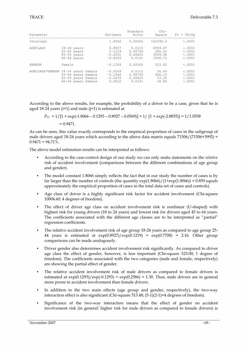
TRACE Deliverable 7.3
November 2007 - 69 -
Standard Chi- Parameter Estimate Error Square Pr > ChiSq ----------------------------------------------------------------------------------- Intercept 1.8066 0.00565 102090.0 <.0001 AGECLASS 18-24 years 0.8927 0.0110 6559.47 <.0001 25-44 years 0.1219 0.00749 265.02 <.0001 45-59 years -0.4591 0.00825 3099.58 <.0001 60-64 years -0.4593 0.0141 1058.72 <.0001 GENDER female -0.1293 0.00565 523.00 <.0001 AGECLASS*GENDER 18-24 years female -0.0569 0.0110 26.60 <.0001 25-44 years female -0.1546 0.00749 426.13 <.0001 45-59 years female -0.0476 0.00825 33.35 <.0001 60-64 years female 0.0612 0.0141 18.80 <.0001
According to the above results, for example, the probability of a driver to be a case, given that he is aged 18-24 years (i=1) and male (j=1) is estimated at
P11 = 1/[1 + exp(-1.8066 – 0.1293 – 0.8927 – 0.0569)] = 1/ [1 + exp(-2.8855)] = 1/1.0558
= 0.9471.
As can be seen, this value exactly corresponds to the empirical proportion of cases in the subgroup of male drivers aged 18-24 years which according to the above data matrix equals 71506/(71506+3992) = 0.9471 = 94.71%.
The above model estimation results can be interpreted as follows:
• According to the case-control design of our study we can only make statements on the relative risk of accident involvement (comparisons between the different combinations of age group and gender).
• The model constant 1.8066 simply reflects the fact that in our study the number of cases is by far larger than the number of controls (the quantity exp(1.8066)/(1+exp(1.8066)) = 0.859 equals approximately the empirical proportion of cases in the total data set of cases and controls).
• Age class of driver is a highly significant risk factor for accident involvement (Chi-square 10004.60; 4 degrees of freedom).
• The effect of driver age class on accident involvement risk is nonlinear (U-shaped) with highest risk for young drivers (18 to 24 years) and lowest risk for drivers aged 45 to 64 years. The coefficients associated with the different age classes are to be interpreted as “partial” regression coefficients.
• The relative accident involvement risk of age group 18-24 years as compared to age group 25-44 years is estimated at exp(0.8927)/exp(0.1219) = exp(0.7708) = 2.16. Other group comparisons can be made analogously.
• Driver gender also determines accident involvement risk significantly. As compared to driver age class the effect of gender, however, is less important (Chi-square 523.00; 1 degree of freedom). The coefficients associated with the two categories (male and female, respectively) are showing the partial effect of gender.
• The relative accident involvement risk of male drivers as compared to female drivers is estimated at exp(0.1293)/exp(-0.1293) = exp(0.2586) = 1.30. Thus, male drivers are in general more prone to accident involvement than female drivers.
• In addition to the two main effects (age group and gender, respectively), the two-way interaction effect is also significant (Chi-square 513.48; (5-1)(2-1)=4 degrees of freedom).
• Significance of the two-way interaction means that the effect of gender on accident involvement risk (in general: higher risk for male drivers as compared to female drivers) is
TRACE Deliverable 7.3
November 2007 - 70 -
not the same for all age groups. For specific age groups the general effect of gender may even be reversed.
• Example: For drivers aged 25-44 years , the relative accident involvement risk of male drivers as compared to female drivers is exp(0.1219 + 0.1293 + 0.1546)/exp(0.1219 - 0.1293 - 0.1546) = exp(0.5678) = 1.76 whereas for drivers aged 65 years and over the corresponding relative risk is exp(-0.0962 + 0.1293 - 0.1979)/exp(-0.0962 - 0.1293 + 0.1979) = exp(-0.1372) = 0.87. Thus, for elderly drivers we find that women are more prone to accident involvement than men.
The logistic model can easily be extended to consider more than two risk factors.
Remark:
Clustering of cases56 and controls57 has not been accounted for in this analysis. Random effects models could be used for this purpose.
56 Two or more car drivers can be involved in the same accident. Therefore, accidents are clusters of road users involved. 57 The set of trips made by a specific person on a given day is to be considered as a cluster.
TRACE Deliverable 7.3
November 2007 - 71 -
Annex III
The Concept of Induced Exposure: An External Validity Check
1. Problem formulation and methodological approach
The concept of induced exposure can be a powerful methodological approach to assess the relative risk of accident causation, provided that the underlying assumptions are sufficiently close to reality. It has been described in Section 6.3.2 that the most frequently applied induced exposure method is built on the assertion that the nonresponsible road users (“innocent victims”) in two-vehicle accidents constitute a random sample from all driver-vehicle combinations on the road system. As under the conceptual framework of this report every accident-involved road user corresponds to an accidental trip, the research question to be answered can be formulated as follows:
May the accidental trips of innocent road users involved in two-vehicle crashes be considered as a random sample from the population of all road user trips?
In response to this question, road user data from German traffic accident statistics have been compared to trip data from the German mobility survey MiD 2002. Both for at-fault and innocent accident-involved car drivers the joint frequency distribution of age and gender has been determined. Similarly, the car driver trips reported in the representative mobility survey were grouped by age and gender of trip maker. For the concept of induced exposure to be considered as valid it is necessary that the empirical age and gender distribution for innocent accident-involved car drivers on the one hand and for car driver trips in general on the other hand do not differ significantly.
This methodological approach corresponds to an external58 validity check. To our knowledge, the first external validity check has been performed by Kirk and Stamiatidis (2001) who developed estimates of travel using a trip diary approach and compared these estimates to the results of the induced exposure approach. However, due to the small number of diaries (26 diaries each with a ten-day reporting period thus leading to a sample of 260 “person-days”) the authors provide only provisional results and conclude that larger samples are necessary for ultimately validating the induced exposure method.
2. Nonresponsible car drivers compared to all car driver trips on the road
From all two-car accidents registered in the German traffic accident statistics 2002 a random sample of 93,820 accidents was selected. Each accident corresponds to a pair of car drivers (responsible and nonresponsible driver, respectively). The joint frequency distribution of driver age (4 classes) and driver gender was determined both for responsible and nonresponsible drivers in the sample.
Similarly, for all car driver trips registered in the German mobility survey 2002 (MiD 2002) the joint frequency distribution of driver age (4 classes) and driver gender was calculated.
The similarity or dissimilarity between the age and gender distribution for accident-involved car drivers on the one hand and all car driver trips on the other hand was measured by the following statistic:
(1) V = √Σ Σ (pij - ij)2/ij
In (1) the symbol pij denotes the proportion of accident-involved car drivers (responsible and nonresponsible drivers, respectively) who belong to age class i and gender class j, whereas ij denotes the corresponding proportion of all driver trips.
58 In the literature predominately validity checks internal to the accident data base can be found. See Stamatiadis and Deacon (1997) and Lyles et al. (1991).
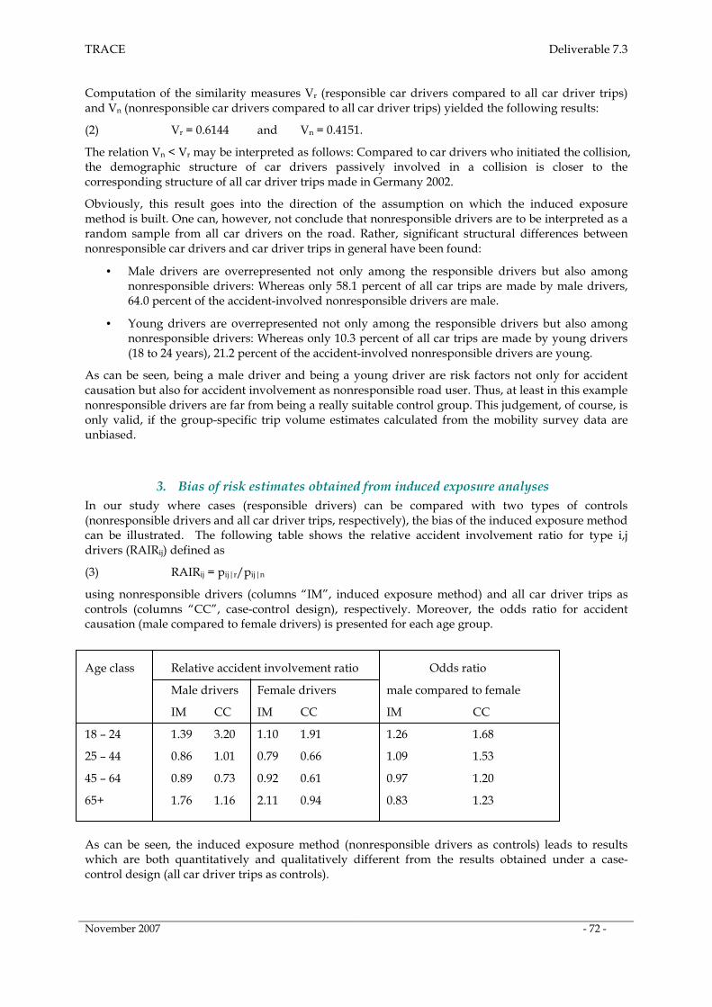
TRACE Deliverable 7.3
November 2007 - 72 -
Computation of the similarity measures Vr (responsible car drivers compared to all car driver trips) and Vn (nonresponsible car drivers compared to all car driver trips) yielded the following results:
(2) Vr = 0.6144 and Vn = 0.4151.
The relation Vn < Vr may be interpreted as follows: Compared to car drivers who initiated the collision, the demographic structure of car drivers passively involved in a collision is closer to the corresponding structure of all car driver trips made in Germany 2002.
Obviously, this result goes into the direction of the assumption on which the induced exposure method is built. One can, however, not conclude that nonresponsible drivers are to be interpreted as a random sample from all car drivers on the road. Rather, significant structural differences between nonresponsible car drivers and car driver trips in general have been found:
• Male drivers are overrepresented not only among the responsible drivers but also among nonresponsible drivers: Whereas only 58.1 percent of all car trips are made by male drivers, 64.0 percent of the accident-involved nonresponsible drivers are male.
• Young drivers are overrepresented not only among the responsible drivers but also among nonresponsible drivers: Whereas only 10.3 percent of all car trips are made by young drivers (18 to 24 years), 21.2 percent of the accident-involved nonresponsible drivers are young.
As can be seen, being a male driver and being a young driver are risk factors not only for accident causation but also for accident involvement as nonresponsible road user. Thus, at least in this example nonresponsible drivers are far from being a really suitable control group. This judgement, of course, is only valid, if the group-specific trip volume estimates calculated from the mobility survey data are unbiased.
3. Bias of risk estimates obtained from induced exposure analyses
In our study where cases (responsible drivers) can be compared with two types of controls (nonresponsible drivers and all car driver trips, respectively), the bias of the induced exposure method can be illustrated. The following table shows the relative accident involvement ratio for type i,j drivers (RAIRij) defined as
(3) RAIRij = pij|r/pij|n
using nonresponsible drivers (columns “IM”, induced exposure method) and all car driver trips as controls (columns “CC”, case-control design), respectively. Moreover, the odds ratio for accident causation (male compared to female drivers) is presented for each age group.
Age class Relative accident involvement ratio Odds ratio
Male drivers Female drivers male compared to female
IM CC IM CC IM CC
18 – 24 1.39 3.20 1.10 1.91 1.26 1.68
25 – 44 0.86 1.01 0.79 0.66 1.09 1.53
45 – 64 0.89 0.73 0.92 0.61 0.97 1.20
65+ 1.76 1.16 2.11 0.94 0.83 1.23
As can be seen, the induced exposure method (nonresponsible drivers as controls) leads to results which are both quantitatively and qualitatively different from the results obtained under a case-control design (all car driver trips as controls).
Top Related