


Languages
Pages
Legal


49AUSTRALIAN JOURNAL OF LABOUR ECONOMICS
Volume 13 • Number 1 • 2010 • pp 49 - 79
Decomposing the Gender Pay Gap in the Australian Managerial Labour Market
Ian Watson,MacquarieUniversity
Abstract This article1 examines the gender pay gap among full-time managers in Australia over the period 2001 to 2008. Using decompositions I explore the issue of discrimination, as well as the roles played by labour force experience and parenting. The results show that female managers earned on average about 27 per cent less than their male counterparts and the decompositions suggest that somewhere between 65 and 90 per cent of this earnings gap cannot be explained by recourse to a large range of demographic and labour market variables. A major part of the earnings gap is simply due to women managers being female. In addition, the presence of dependent children worsens the earnings gap, while the financial returns to labour force experience diminish in the latter years among female managers rather than stabilising, as they do for male managers. Despite the characteristics of male and female managers being remarkably similar, their earnings are very different, suggesting that discrimination plays an important role in this outcome. The article uses eight waves of HILDA data to fit mixed-effects models which are then used for Blinder-Oaxaca decompositions. In addition, a recent simulated change approach, developed by Olsen and Walby in the UK, is also implemented using this Australian data.
JELClassification:J31,J70,J16
1ThisarticleusesunitrecorddatafromtheHousehold,IncomeandLabourDynamicsinAustralia(HILDA)Survey.TheHILDAProjectwasinitiatedandisfundedbytheAustralianGovernmentDepartmentofFamilies,Housing,CommunityServicesandIndigenousAffairs(FaHCSIA)andismanagedby theMelbourne InstituteofAppliedEconomic andSocialResearch (MIAESR).Thefindingsandviewsreportedinthisarticle,however,arethoseoftheauthorandshouldnotbeattributedtoeitherFaHCSIAortheMIAESR.
Address for correspondence: Ian Watson, Senior Research Fellow, Politics and InternationalRelations,MacquarieUniversity,Sydney,NSW,2109.Email:[email protected]: Iwould like to thankElkeHolst (DIW,Berlin) for suggesting this study,whichwasoriginallyintendedtobeajointprojectcomparingGermanyandAustralia.Illhealthpreventedourcollaborationbutherinspirationismuchappreciated.IwouldalsoliketothanktherefereeandeditorfortheirvaluablefeedbackandMarkWoodenandparticipantsattheHILDA2009ResearchConferencefortheirusefulcomments.©TheCentreforLabourMarketResearch,2010

50AUSTRALIAN JOURNAL OF LABOUR ECONOMICSVOLUME 13 • NUMBER 1 • 2010
1. Introduction Untiltheearly1970sthegenderpaygap2inAustraliawaswide,andwaskeptthatwayby‘institutionalisedgenderwagediscrimination’,inthewordsofPaulMiller(1994,p.371).Thehistoricequalpaydecisionsof1969,1972and1974endedthis,andhelpedclosethegapconsiderably(see,forexample,GregoryandDuncan,1981;andBorland,1999).Nevertheless,agenderpaygapofconsiderablesizehasremainedtothisday.In his overviewat the endof the1990s,Borland summarised a numberof studiescovering the1980sand1990swhichshowed that thepaygaprangedfromabout8percentto25percent(Borland,1999,p.267).Borlandobservedthatdiscriminationaccountedforbetween7percentagepointsand19percentagepointsofthegap.Heconcludedthatmostofthereductioninthepaygapsincetheearly1970swasduetoa‘decreaseinwagediscrimination’(Borland,1999,p.268).
Theearlyequalpaycasesdidnotfullypursuethelabourmarketdimensionof the gender pay gap, particularly occupational-based gender segregation. By the1990s, thishadbecome the focus forpayequity inquiries inwhich the conceptofcomparableworthwasacentralplank(Pocock,1999).Usingdatafromthelate1980s,Miller(1994)foundagenderpaygapofabout13percent,withalargecomponentofthatgap(6percentagepoints)duetooccupationalconcentration.AsMillernoted:‘about40percentofthedifferentialmightberemovedbytheimplementationoftruecomparableworth’ (1994, p. 367).Using a comparable, but later data set,Wooden(1999)alsoexaminedtheissueofcomparableworth.WhiletheactualpaygapwassmallerinWooden’sstudy(11.5percent),hisresultswerebroadlysimilartoMiller’s.Woodenfoundthatoccupationalconcentrationaccountedfor4.2percentagepoints,thatis,aboutonethirdofthegap(1999,p.167).
However,Wooden argued that including themanagerialworkforce in suchstudies was unwarranted.When he removedmanagers from the sample, he foundthat the gender pay gap fell to 8.9 per cent, with the occupational concentrationcomponentnowaccountingfor3.6percentagepoints.Woodennotedthattheunder-representationofwomeninseniormanagementpositionsinAustraliancompanieswaslikely towiden thegenderpaygap,becausemanagers earnedmuchmore than theall-occupationalaverage.Asaconsequence,heconcluded,thisremovedthescopeforindustrialtribunalstoeliminateaconsiderablepartofthegenderpaygapbecause‘theearningsofmanagerstypicallylieoutsidethepurviewofindustrialawards’.Woodenfurtheradded,‘theproblemisnotnecessarilyoneofunequalearnings,butratherofunequalaccesstopromotion’(Wooden,1999,p.167).
While much of the research on the gender pay gap has focussed on theworkforcemoregenerally,orat least the full-timeworkforce, recent studieshavebegun toexamine thegapacross theentirewagesdistribution.Usingunit recorddatafromthe2001Australiancensus,PaulMillerfoundthatthepaygapwasmuchgreateramonghighwageearnersthanamonglowwageearners.Inthe5thtothe35thquantileitwasbelow10percent,atthe40thquantileitwasabout12percent,
2Theterms‘wages’,‘pay’and‘earnings’areusedinterchangeablyinthisarticletorefertolabourmarketearnings.Theterm‘wages’ismorecommonlyusedwhendiscussingthedecompositionliterature, or the labour force more generally; the term ‘pay’ is preferred when discussingmanagerialearnings,where‘wages’seemsasomewhatinappropriateexpression.

51IAN WATSON
Decomposing the Gender Pay Gap in the Australian Managerial Labour Market
butatthe95thquantileitreached23percent(2005,p.412).ThisledMillertoargue:‘whilethepolicydebateonthegenderwagegapneedstofocusonallpartsofthewagedistribution,thereisaparticularneedforattentionamonghigh-wageearners’(2005,p.412).Moreover,other researchsuggests thatpolicy initiativesmayworkdifferently at different locations in the distribution. As Gardeazabal and Ugidos(2005,p.167)argue:
...policies might have different impacts at different quantiles ofthedistributionofwages if, forexample, asa resultof thepoliciesimplementedmorewomenenterintolowpaidoccupations.Therefore,it is necessary tomeasure genderwage discrimination at differentquantilestodeterminetheindirecteffectofsuchpolicies.
Innovationsintheuseofquantileregressionmethods(forexample,Buchinsky,1998;andKoenkerandHallock,2001)haveopenedupthisfieldofresearch.UsingthefirstwaveoftheHILDAdata,Kee(2006)madeuseofquantileregressiontoexplorethegender paygap inAustraliawhileAlbrechtet al. (2003),Gardeazabal andUgidos(2005) andArulampalamet al. (2007) haveusedquantile regression coupledwithdecomposition methods to unpack the gender pay gap in Sweden, Spain, and theEuropeanUnion,respectively.
Otherdecompositionapproacheswhichdon’tinvolvequantileregressionhavealso examined the gender pay gap inAustralia at different locations in thewagesdistribution.RecentresearchbyBarónandCobb-Clark(2008),usingsemi-parametricmethodsdevelopedbyDiNardoet al.(1996),havepursuedthisstrategyusingthefirstsixwavesoftheHILDAdata.Astheseauthorsobserved:
itisnowbecomingclearthatthemagnitudeofthegenderwagegapisgenerallynotconstantacrosstheentirewagedistributionandthatthegapinmeanwagesobscuresagreatdealoftheinterestingvariationinthedata...amuchricherstoryabouttheroleofgenderinthelabourmarket emerges once we move away from an exclusive focus onoutcomesfor‘average’menandwomen(2008,p.2).Barón and Cobb-Clark (2008) contrasted the private and public sectors, a
strategywhichKee(2006)hadalsoearlierpursued.Keefoundthatthegenderpaygapincreasedathigherlevelsintheprivatesector–leadingtoherconclusionthataglassceilingexistedthere–butthatthegapinthepublicsectorwas‘relativelyconstant’overallpercentiles(Kee,2006,p.424).Whiletheirmethodsdiffered,thestudybyBarónandCobb-Clark(2008)reinforcedKee’sfindingthatthegapwas‘roughlyconstant’acrossthepublic-sectorwagesdistribution–atabout13percent–buttheyalsofounda somewhat surprising resultwhich reflected poorly on public sector employment.Their decompositionmethod showed that the explanation for thepublic-sector gapwashighlysensitivetolocationwithinthewagesdistribution,withtheunexplained(ordiscriminatory)componentofmuchgreaterinfluenceatthetopofthedistribution:

52AUSTRALIAN JOURNAL OF LABOUR ECONOMICSVOLUME 13 • NUMBER 1 • 2010
Theproportionof thegenderwagegap thatcannotbeexplainedbydifferencesinwage-relatedcharacteristicsisinsignificantlydifferentfromzero in thebottomhalf of thedistribution.Amonghigh-wageworkers, however, the portion of the wage gap not attributable togenderdifferencesinendowmentsrisestoover90percent.Despitethe fact that themagnitudeof thepublic-sectorgenderwagegap isrelatively constant, the extent to which it can be explained by thewage-relatedcharacteristicsofmenandwomenfallsaswemoveupthewagedistribution.Overall,itappearsthathigh-wagepublic-sectoremployeesinAustraliamayfacemoreemployerdiscrimination(i.e.,glassceilings)thanlow-wageworkers(i.e.,stickyfloors)(2008,p.17).3
Intheprivatesector,ontheotherhand,theyfoundthattheunexplainedcomponentattopofthedistributionismuchsmaller–atbetween50and60percent–suggestingdiscriminationwaslessinfluential(thoughstillofaconsiderablemagnitude).
InthisarticleIbuilduponthistraditionofdecomposingthepaygapatthetop of the wages distribution. However, rather than contrasting different locationswithinthatdistribution,Ifocusspecificallyontheoccupationalgroupingofmanagers.DefinedaccordingtotheANZSCOMajorGroup1,thisoccupationisquitedistinctiveandlendsitselftoagendercomparisonofearnings.Theworkwhichmaleandfemalemanagers do is highly comparable and there is no obvious reason for any kind ofsub-occupationalsegregation.Levelsoffull-timeworkamongfemalemanagersareexceptionally high, while the educational levels ofmale and femalemanagers areremarkably similar. At the same time, however, the top echelons of managementare disproportionately occupied bymen, returning us toWooden’s point about theassumedlinkbetweeninequalityinaccesstopromotionandthegenderpaygap.
Atnotedearlier,someofthedecompositionliteratureinthisareahasfocusedon quantile regression. There are, in addition, several studies which have useddecompositionmethodstounpackthegenderpaygapinthemanageriallabourmarket.TheseincludeLausten(2001)andHolstandBusch(2009)forDenmarkandGermanyrespectively. The former used a combined gender and occupational decompositionapproachandestimated theunexplained (ordiscriminatory)portionof thepaygapat between 23 per cent and 32 per cent (2001, p. 21). Holst and Busch compareddecompositionswithandwithoutselectioneffects (that is, taking intoaccountwhobecomesamanager).Inclusionoftheselectioneffecthadamajorimpact,increasingtheunexplainedportionofthegenderpaygapamongmanagersfromabout30percenttotwo-thirds(2009,p.26).
It is reasonable to regard the level of annual earnings as a roughproxy forsenioritysotheproblemofthegenderpaygapamongmanagersalsoraisesquestionsaboutdiscriminatoryoutcomes in long-termcareerpathsbetweenmenandwomen.Inotherwords,thephenomenonoftheglassceiling–whichblocksthemovementofwomenfrommiddleintoseniormanagement–appears tobeanintegralpartof the
3Stickyfloorsrefertothesituationwherethegenderwagegapwidensatthebottomofthewagedistributionandglassceilingsrefertothesituationwhereitwidensatthetop(seeArulampalamet al.,2007,p.164).

53IAN WATSON
Decomposing the Gender Pay Gap in the Australian Managerial Labour Market
genderpaygapatthislevelofthelabourmarket.Byunpackingsomeofthedeterminantsofthegenderpaygap,usinganumberofdifferentdecompositionmethods,itshouldbepossibletogaininsightsintothisdimensionofgenderinequalitywithinthemanageriallabourmarket.Inparticular,weknowthatitiscommonforwomen–butinfrequentformen–toexperienceparentingasamajordisruptionintheirworkinglives.Whilethismayormaynottranslateintofragmentedcareerpaths,itdoesrepresentfragmentationin the duration and continuity of their job and labour force experience (Beblo andWolf,2002).Theconventionalearningsequationswhichexaminethereturnonyearsofexperiencehaveoftenusedageasaproxyforexperience,astrategywhichoverlooksthisimportantgenderdifference.Fortunately,theHILDAdatasetusedforthisstudymakesuseofavariablewhichdirectlymeasuresyearsoflabourforceexperienceandavoidsthisgenderbias.Thisprovidestheopportunityinthisarticletoaddressakeyresearchquestion.Amongthedeterminantsofthegenderpaygap,whatrolesdolabourforceexperienceandparentingplayininfluencingthisoutcome?
AswiththeBarónandCobb-Clark(2008)study,myanalysismakesuseoftheHILDAdata.Intermsofmethod,thedecompositionapproachusedhereinvolvestwo different strategies.While they both assist in quantifying the extent towhichthe gender pay gap is based on discrimination, they do so in different ways. Thefirst strategyusesBlinder-Oaxacamethods toprovideadetailedbreakdownof thevariableswhichcontributemosttothediscriminatorycomponentwithinthegenderpaygap.Thesecondstrategymakesuseofasimulatedchangemethodology,developedbyWendyOlsenandSylviaWalbyintheUnitedKingdom(OlsenandWalby,2004;andWalby andOlsen, 2002).This also allows for a detailed decomposition and itmakes itpossible to render thecontributionof individualvariables indollar terms.Withthisstrategyresearcherscanexamine,forexample,howmuchtheirparentingroles costwomen in dollar terms.Both of these strategies point towards the sameconclusion:simplybeingafemaleisthebasisforthemajorpartofthegenderearningsgapfoundamongmanagers.Atthesametime,familylifeandlabourforceexperiencearepivotal inunderstandingunequaloutcomesinthemanagerial labourmarket.Insummary,bothdirectandindirectformsofdiscriminationappeartobeimplicatedinthemaintenanceofthegenderpaygap.
2. Method The Blinder-Oaxaca Tradition of Decomposing Wage Gaps The use of Blinder-Oaxaca decompositions have been a mainstay of sociologicalandeconomicanalysisforthelast35years.Sincetheirpioneeringworkintheearly1970s, the coremethod ofBlinder (1973) andOaxaca (1973) has been reproducedmanytimes,thoughwithvariationsandextensionstoaccommodatemethodologicalweaknessesanddifferentassumptions.Thecore technique isquitestraightforward.Afterfitting separate regressions formales and females, thepredictedwagegap isdecomposedintothatcomponentbasedonthedifferingcharacteristicsofeachgroup,andanothercomponentbasedonhowthosecharacteristicsarerewardedinthelabourmarket (the regression coefficients). Only the difference in characteristics can bereadilyexplained,andinthissense,theunexplainedportionofthewagegapcanberegardedasdiscriminatory.Fromwithinahumancapitalframework,thedifferences

54AUSTRALIAN JOURNAL OF LABOUR ECONOMICSVOLUME 13 • NUMBER 1 • 2010
in characteristics have usually been referred to as a difference in ‘endowments’(Blinder, 1973)or as a ‘productivitydifferential’ (OaxacaandRansom,1994).Theunexplainedcomponenthasbeenvariouslyreferredtoasthe‘coefficientseffect’or,moregenerally,the‘discrimination’component.
Whileitiscommontoseetheterminologyof‘endowments’(or‘productivitydifferential’)and‘discrimination’usedthroughouttheliterature,itisimportanttokeepinmindseveralcaveatsaroundtheseterms.Thefirstsetoftermsarebasedonhumancapitalassumptionsaboutwagesandproductivity,assumptionsnotuniversallysharedamonglabourmarketresearchers.Clearly,amoreneutraltermlike‘characteristics’ispreferable.Theterm‘discrimination’canbemisleading:withinthedecompositionmethoditisonlyeveridentifiedasaresidual,thepartthatcannotbeexplainedbythecharacteristicsofthesample.InthewordsofDoltonandMakepeace(1986,p.332),‘theresidualisreallyameasureofourignorance’.Whilerecognisingtheimportanceofthiscaveat,Iwillcontinuetousetheterm‘discrimination’becauseitissocentraltothistraditionofresearch.
Thecoredecompositionmethodcanbeillustratedasfollows.Thewagegapbetween the twogroupscanbeviewedas thedifference in thepredictedmeansofthe(natural)logsofmale(m)andfemale( f)wages.Followingthefittingofseparateregressionfunctions,itcanberepresentedby:
w^m- w^
f=∑bm X-
m - ∑bf X-
f(1)
where the bs are the regression coefficients and the X-s are the vectors of mean
characteristics.Rearranging the terms, and representing thewage gap byGmf, it isstraightforwardtoshowthatthereareatleasttwowaysofdecomposingthiswagegap:
Gmf =∑bf (X-
m - X-
f)+∑X-m(bm - bf ) (2)
and
Gmf =∑bm (X-
m - X-
f)+∑X-f(bm - bf ) (3)
Ineachcase,thefirstpartoftheright-handsidesoftheseequationscontainestimatesofthedifferencesinthecharacteristicsofmalesandfemales,weightedbythefemale(2)andmale(3)coefficients.Inotherwords,thedifferencesinthecharacteristicsofeachgrouparerewardedaccordingtothewagestructureoffemalesormales(dependingonwhichdecompositionisused).Thesecondsetoftermsintheseequationscapturethe‘discrimination’component:theymeasurethedifferencesineachwagestructure–howthelabourmarketdifferentiallyrewardseachgroup–appliedtothemale(2)andfemalecharacteristicsrespectively(3).SeeNeumark(1988,p.281)andCotton(1988,p.236)formoredetails.
Itisclearfromthesetwoequationsthatakeychoicewithinthedecompositiontraditionisanormativecriterion,thatis,adecisionaboutwhatshouldconstituteanon-discriminatory benchmark against which toweight the differences. Regarding thecurrentfemalewagestructureasnondiscriminatoryleadstoamodelofdiscrimination

55IAN WATSON
Decomposing the Gender Pay Gap in the Australian Managerial Labour Market
inwhichmalesearnmorethantheyshould.Ontheotherhand,regardingthecurrentmalewagestructureasthenormimpliesamodelofdiscriminationinwhichfemalesearn less than they should.Muchof the literature subsequent to the earlywork ofBlinder and Oaxaca has concentrated on examining different non-discriminatorybenchmarks. These have gone beyond equating non-discriminationwith either themaleorfemalewagestructure.Reimers(1983,p.573),forexample,suggestedthatina‘nondiscriminatoryworld’thewagestructurebywhichtoweightthedifferenceswouldmostlikelyliesomewhereinbetween.Cotton(1988,p.238),inthecontextofraciallybasedwagegaps,tookasimilarview:
...not only is the group discriminated against undervalued, but thepreferred group is overvalued, and the undervaluation of the onesubsidizestheovervaluationoftheother.Thus,thewhiteandblackwagestructuresarebothfunctionsofdiscriminationandwewouldnotexpecteithertoprevailintheabsenceofdiscrimination.
Where Reimers took the average difference between the male and female wagestructures,Cottonweightedthewhiteandblackwagestructuresbytheproportionsofeachgroupinthelabourforce(1988,p.239).Fromadifferentperspective,Neumark(1988)regardedthesebenchmarksasunsatisfactoryandarguedthatthechoiceofanon-discriminatorywagestructureshouldbebasedontheoreticalgrounds.UsingBecker’stheoryofemployerdiscrimination(Becker,1971),Neumarkderivedan‘estimableno-discriminationwagestructure’(1988,p.283)whichheusedashisweightingscheme.InasimilarfashionOaxacaandRansom(1994,p.9)criticisedbothReimersandCottonforadoptinganon-discriminatorywagestructurewhichwasbasically‘arbitrary’.LikeNeumarktheyproposedastheirnon-discriminatorywagestructureaweightingmatrixbasedontheordinaryleastsquares(OLS)estimatesfromapooledregression(ofbothmalesandfemales),arguingthatthesepooledestimatesreflected‘thewagestructurethatwouldexistintheabsenceofdiscrimination’(1994,p.11).
Thesemethodsaresummarisedintable1,whichdrawsuponthepresentationofresultsdevelopedbyOaxacaandRansom(1994,p.13).Itisusefulbecauseitmakesthenon-discriminatorybenchmarkexplicit,anditalsoshowsthattheunexplainedordiscriminatorycomponentcanbefurtherdecomposed:
Gmf =∑b* (X-
m- X-
f)+∑X-m (bm - b*) +∑X-f (b*- bf ) (4)
Hereb* makesexplicitthenon-discriminatorywagestructure.Asbefore,the
firsttermontheright-handsideshowsthedifferencesinmaleandfemalecharacteristicsweightedbyaparticularwagestructure,inthiscase,thenon-discriminatorybenchmarkb*.Thesecondandthirdtermsrepresentthelastpartofequations(2)and(3)inwhichthe unexplained component is now decomposed into that partwhich reflectsmaleprivilegeandthatpartwhichreflectsfemaledisadvantage.ThelasttwocolumnsinTable1showtheweightingmatrixwhichisappliedineachofthemethodslisted.Thediagonalsofthismatrixconsistofeither1sor0s(identitymatrixandnullmatrix)inthefirsttwomethods;asetofratios(0.5andthefemale-maleratio)intheReimers
56AUSTRALIAN JOURNAL OF LABOUR ECONOMICSVOLUME 13 • NUMBER 1 • 2010
andCottonmethod;andasetofweightsbasedonthedifferencesbetweenthepooledregressioncoefficientsandtheseparatemaleandfemaleregressioncoefficients(theNeumarkandOaxacaandRansommethods).
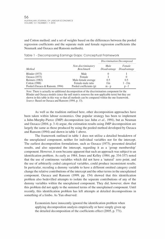
Table 1 - Decomposing Earnings Gaps: Conceptual Framework
Discrimination Decomposed Non-discriminatory Male FemaleMethod Benchmark Disadvantage DisadvantageBlinder(1973) Male 0 IOaxaca(1973) Female I 0Reimers(1983) Male-femaleaverage 0.5 0.5Cotton(1988) Female-maleratio f/m 1-f/mPooled(Oaxaca&Ransom,1994) Pooledcoefficients(p) m-p p-f
Note:ThereisactuallynoadditionaldecompositionofthediscriminationcomponentfortheBlinderandOaxacamodels(sincethenullmatrixremovesthenon-applicableterm)buttheyareshowninthistableinthiswaysothatallmethodscanbecomparedwithintheoneframework.Source:BasedonOaxacaandRansom(1994,p.13).
Aswellasthetraditionoutlinedhere,otherdecompositionapproacheshavebeen takenwithin labour economics.One popular strategy has been to implementaJuhn-Murphy-Pierce(JMP)decomposition(seeJuhnet al.,1991),butasNeumanandOaxaca(2004,p.3-4)argue,theestimationresultsusingJMPdecompositionarelargelythesameasthoseproducedbyusingthepooledmethoddevelopedbyOaxacaandRansom(1994)andshownintable1above.
Theframeworkoutlinedintable1doesnotutiliseadetailedbreakdownofthe unexplained component, neither for individual variables nor for the intercept.Theearliestdecompositionformulations,suchasOaxaca(1973),presenteddetailedresults, and also separated the intercept, regarding it as a ‘group membership’component.However,itsoonbecameapparentthatsuchanapproachwassubjecttoanidentificationproblem.Asearlyas1984,JonesandKelley(1984,pp.334-337)notedthat theuseof continuousvariableswhichdidnothave a ‘natural’ zeropoint, andtheuseofarbitrarilycodedcategoricalvariables,couldproduceinconsistentresults.Inparticular,recodingadummyvariabletohaveadifferentomittedcategorycouldchangetherelativecontributionsoftheinterceptandtheothertermsintheunexplainedcomponent. Oaxaca and Ransom (1999, pp. 154) showed that this identificationproblemalsobedevilledattempts to isolate theseparatecontributionsofanyof thedummyvariableswithin theunexplainedcomponent.Theydid,however,showthatthisproblemdidnotapplytothesummedtermsoftheunexplainedcomponent.Untilrecently, this identificationproblemhas left attempts at detaileddecompositions insomethingofalimbo.AsYunobserved:
Economistshaveinnocentlyignoredtheidentificationproblemwhenapplyingdecompositionanalysisempiricallyorhavesimplygivenupthedetaileddecompositionofthecoefficientseffect(2005,p.771).

57IAN WATSON
Decomposing the Gender Pay Gap in the Australian Managerial Labour Market
Yun herself provides one solution, as do Gardeazabal and Ugidos (2004,p. 1035): use a normalized equation and employ themean characteristics of eachcategorical variable. Yun does this through a restricted least-squares estimationapproach(2005,p.771),whileGardeazabalandUgidos(2004,p.1035)achievethesamegoalbyrestrictingthecoefficientstosumtozero,thatis,throughatransformationofthedummyvariables.Inpracticethisamountstousingso-calleddeviationcontrastcoding, such that for any particular categorical variable, the coefficient of eachcategoryreflectsadeviationfromthegrandmean.Thisistheapproachadoptedinthisarticleforproducingthedetaileddecompositiontableshownbelow.4
A Simulated Change Approach AsnotedearliertheBlinder-Oaxacatraditionisnottheonlywaytodecomposethegenderpaygap.A recent innovationdevelopedbySylviaWalbyandWendyOlsenintheUK(WalbyandOlsen,2002;andOlsenandWalby,2004)hasemphasisedtheimportanceofpooledregressions,ratherthantheseparateregressionswhichareatthecoreofmanyofthetraditionalmethods.5Astheyargue:‘usingseparateregressionsforwomenandmenimpliesuntenableassumptionsastotheseparationofmaleandfemalelabourmarkets’(OlsenandWalby,2004,p.5).
TheapproachdevelopedbyOlsenandWalby(2004,pp.63-70)entailsfittinga pooled regression and then using simulated changes in the characteristics of thesample to quantify the contribution made by gender to the actual wages gap. Inpractices,onemultipliesthe(pooled)modelcoefficientsbythegenderdifferenceinthemeanvaluesforeachofthevariablesinthemodel.Intheirframework,thewagegapcanberepresentedby:
w-m - w-
f=∑b9∆X (5)
where∆Xrepresentsthedifferenceintwomeans(x-m- x-
f )foreachvariable.Inthecaseofdummyvariables–suchasgenderitself–thedifferencerepresentsaswitchfromonecategorytoanother(e.g.maletofemale).OlsenandWalbyterm∆Xa‘changefactor’andbymultiplyingitbyβtheycalculatea‘simulationeffect’(thatis,b9∆X).This simulation effect can be expressed as a percentage of the pay gap, and also,conveniently,asamonetaryequivalentoftheactualpaygap.Table10belowillustrateshowthisworksinpractice.
Olsen andWalby note that their approach is similar to using standardisedregression coefficients, but without the incoherent treatment of binary variablesentailedinthatmethod.Instead,anexplicitsimulation,inwhicheachvariableistreatedsubstantivelyandisexaminedtoseehowfarareasonablehypotheticalchangewouldaffecttheoutcome,isevenbetterthanbetacoefficients(OlsenandWalby,2004,p.69).
Onecanapply this approach toallof thevariables in the regression,or to4Notethatalltheregressionresultsshownintheappendixusethemoreconventionaltreatmentcontrastcoding,sincetheinterpretationofdichotomousdummyvariablesismorestraightforward(forexample,thecoefficientisasimplecontrastwiththeomittedcategory,ratherthanacontrastwiththeaveragebetweenthetwo.)5WiththeexceptionofOaxacaandRansom(1994)andNeumark(1988)whoalsousedpooledregressions,asshowninthelastrowoftable1.

58AUSTRALIAN JOURNAL OF LABOUR ECONOMICSVOLUME 13 • NUMBER 1 • 2010
just a subset.Olsen andWalby, for example, argue that somevariables should justberegardedascontrols(suchasindustry)whileothersareregardedashavingmorepolicyrelevance(suchasworkinghoursoreducation).Byhypothesisingachangeinthelatter,theresearchercanexaminethosefactorswhichinfluencethewagesgapandwhichareamenabletopolicyinitiatives.Inpractice,thisapproachmakesitpossibletoestimatethechangeinearnings‘thatwouldoccurifwomen’sconditionschangedtoreflectthebestortheaveragesituationamongmen’(OlsenandWalby,2004,p.66).Asanexample,onecanexaminethesimulationeffectofanyparticularvariable–suchasyearsofpart-timework–andexpressthisasapercentageofthepaygap.UsingBritishHouseholdPanelSurveydata,OlsenandWalby(2004,p.65)foundthatthisparticularvariablehadasimulationeffectof0.02,whichaccountedfor10percentoftheirgrosswagesgapof0.23.Thisvariablecouldthenbegivenamonetaryvalue,namely24penceperhour(10percentofthe£2.28wagesgap).Inthefinalsectionofthisarticle,IimplementtheOlsen/WalbyapproachandillustrateitsrelevanceintheAustraliansetting.
Sample Selection Bias Thesampleofpersonsunderscrutinyinthisarticleareonlyasubsetofallpersonscontained in the HILDA survey dataset. Only employees working as full-timemanagersareincludedinthemodellingdatasetandtheseexclusionshaveimportantimplicationsforfittingearningsequations.Themodellingmustdealwithproblemsof sample selection bias, that fact that only a subset of individuals are observedwithin this category of interest, and only some of these are observed in all years.The reason selectivitymatters is that the factorswhich influenceselection into thesamplemaytobecorrelatedwiththeregressorswhichpredicttheoutcomeofinterest,namely earnings. If such factors are observable, then they can be included in theregressionmodelandbiasintheestimatescanbeovercome.However,thepossibilitythatunobservablefactorsinfluenceselectionintothesampleremainsanobstacle.Alargeliteraturehasevolveddevotedtothisproblem(see,forexample, theoverviewinVella,1998).Theissueisparticularlypertinenttostudiesofwomen’swages,giventhelabourforceparticipationdecisionsentailed(see,forearlyexamples,DoltonandMakepeace,1986; andBloomandKillingsworth,1982).Sample selectionbiaswasalsoanobviousissueconfrontedatanearlystageinthedecompositionliterature(forexample,Reimers,1983).
ThisissueisdealtwithinthisstudythroughtheuseoftheHeckman(1979)two-stepapproachbyfittinga selectionmodel to thedataprior tofitting themainearningsequation.Theselectionequationseekstomodelwhobecomesamanager–usingmultinomiallogitestimation–andisusedtoconstructacorrectionterm(theinverseoftheMillsratio)whichisthenincludedwiththeotherregressorsinthemainearningsequation.Ifthiscorrectiontermisnotstatisticallysignificant,thenonecanconcludethatselectionbiasisnotanimportantissueandmodellingtheearningscanproceedwithouttheneedforincludingthecorrectionterm.Inthecaseofthisstudy,thiswasthecase,andthecorrectiontermwasexcludedfromthefinalmodelsusedforthedecompositionanalysis.6AsBarónandCobb-Clark(2008,p.6)suggest,studies
6Forreasonsofspace,thefulldetailsoftheselectionequationmodellingusedforthisarticlearenotshownherebutareavailablefromtheauthor.

59IAN WATSON
Decomposing the Gender Pay Gap in the Australian Managerial Labour Market
basedonpaneldataarelesslikelytofindselectioneffectsthanthosebasedoncross-sectional data.Longitudinal data, particularly for a largenumberofwaves, clearlyincreasestherangeofindividualswhoareobservedoverthescopeofthestudy.ThismaypartlyexplainthedifferentresultsobtainedbyHolstandBusch(2009),whofindselectioneffectshaveamajorimpactontheircross-sectionaldecompositionresults.
Panel Data and Mixed-effects Modelling There are a number of advantages in using panel data for this study. Because thecategoryof interest issuchasmallgroup–full-timeadultmanagers–samplesizeconsiderationsareparamount.Therearemajorgainsintheprecisionoftheestimatesforthedecompositionresultsfromusingalargernumberofobservationsfrompoolingthedataacrossallwaves.Moreover,theuseofmixed-effectsmodellingwithpaneldataalsoprovidesmoreconsistentestimatesandhelpsdealwithunobservedheterogeneity.
Mixed-effectsmodels, also calledmultilevelmodels, entail fitting amodelwith afixedcomponent– theusual set of earnings regression controls – aswell arandomcomponent(PinheiroandBates,2004;andGelmanandHill,2007).Theactualdatasetobservationscanberegardedas‘earningsepisodes’whichareclusteredwithinindividuals. This hierarchical structure induces dependence among observations,violatingoneofthekeyassumptionsofordinaryleastsquaresregression.Whileonecanpartiallydealwith thisusingvarious robust estimators to correct the standarderrors, a more rigorous approach attempts to model the variance directly.Mixed-effectsmodellingprovidesforthisbyallowingforarandomeffectattheleveloftheindividualandbyallowingforthemodellingofthevarianceandthecovariancewithintheearningsepisodesaswell.
Thisapproachavoidsthepitfallsofcompletepoolingofpaneldata–whichwouldleadustoignoredifferencesbetweenindividualsandandsuppressvariationinthedata–and,ontheotherhand,nopoolingwithitsproblemsofunreliableestimates(Gelman andHill, 2007, pp. 7, 256). Amixed-effects approach can also deal withunbalanced panel data, such as when there is only one observation per individualsubject.InthecaseoftheHILDApanelofmanagersusedinthisstudy,therearealargenumberofindividualswhoonlyappearonceinthepanel,withfemalesmorelikelytobeinthissituation(53percent)thanmales(44percent).Theiromissiondoesnotjustreflect absence from the labourmarket, but occupationalmobility, and the fact thatbecomingamanagerisusuallysomedistancealonganindividual’scareerpathway.7
Thecoefficientsforthefixed-effectsfromthemixed-effectsmodelareusedasthebasisforthedecompositionoftheearningsgapwhilepredictionsfromthemodelareusedtoexplorereturnstolabourforceexperience.Foramixed-effectsmodel,theearningsequationtakestheform:
yit=Xit b+ui+eit(6)
whereyit is thelogannualearningsforeachindividual i, inperiod t.ThetermsXit andb are theusualmatrixof covariates and thevector ofmodel coefficients.Therandomcomponentisexpressedthroughtheui term,andeit istheidiosyncraticerrorterm (the residual). The former captures the random intercepts dimension of the

60AUSTRALIAN JOURNAL OF LABOUR ECONOMICSVOLUME 13 • NUMBER 1 • 2010
modelling–at the levelof the individual–while the lattercaptures thevariabilityaround each earnings episode. This residual is assumed to have an autoregressivecorrelationstructureoforderone(AR1).Inotherwords,theerrortermforearningsinadjacentyearsisassumedtobemorehighlycorrelatedthanthoseseparatedbyalargernumberofyears.Thedecompositionmethodworkswiththefixedeffectsfromthismodel,whichisthesamestrategyusedforestimatingmarginalpredictionsfrommixed-effectsmodels(PinheiroandBates,2004;andWestet al.,2007).Theactualdecompositionroutineisthuslittledifferenttothatwhichapplieswhendecomposingaconventionalordinaryleastsquaresregression.
Summary statistics for the variables used for the regressionmodeling canbe found in table11 and the regression coefficients and standard errors are shownintable12.Themixed-effectsmodelswerefitusingrestrictedmaximumlikelihoodestimation(REML)andmadeuseofthelmeandlmerfunctionsfromthenlmeandlme4packagesusingtheRstatisticalenvironment(Pinheiroet al.,2009;andBatesandMaechler,2009;andRDevelopmentCoreTeam,2009).Mostoftheexplanatoryvariablesrepresenttheusualearningsequationvariables,codedintheconventionalwaybutwithafewvariations.Yearsoflabourforceexperience,definedasthenumberofyearsinpaidwork,includedacubic,aswellasasquaredterm.Thiscapturestheusualplateauingofearningsthatoccursinthelatteryear,butmoderatesthedrop-offattheverytopend(atendencywhichisempiricallyappropriateformanagerialoccupations).The inclusionofexperiencerequired thatagebeomitted(due tohighcollinearity).Someoftheusualindustrycategorieswerecollapsed(forexample,constructionandutilitieswerecombined,aswerewholesaleandtransport)becauseofthesmallnumberofwomenmanagersintheseblue-collarindustries.Forreasonsofsamplesizeseveralofthestateswerecombined.Finally,afinermeasureofoccupationaldifferentiationwithinthebroadermanagerialcategoryofANZSCOMajorGroup1wasintroducedbyemployinganoccupationalstatusvariable.
Asmentionedearlier,theselectivity-correctedmodelsprovedunnecessarysotheresults reportedheredealonlywith thefinalmixed-effectmodels.Modelswerefitseparatelyformalesandfemalesandinterestcentredontheearningsdifferentialbetweenmalesandfemales,andhowthismightbedecomposedinvariousways.Inordertoallowforapooleddecomposition–theOaxacaandRansom(1994)method–andinordertoimplementtheOlsen-Walbyapproach,amodelusingpooledmaleandfemaledatawasalsofit.FollowingJann (2008,pp.457-458), adummyfor sexwasincludedinthepooledsample,toavoidpossibledistortionofthedecompositionresults.
7Isarandominterceptsmixed-effectsmodelappropriatewhenlargenumbersofindividualshaveonlyoneearningsepisode?AccordingtoGelmanandHill(2007,p.276),suchmodelsarecertainlyfeasible;whileforWestet al.(2007,p.48)onlyifthe‘vastmajority’ofsubjectshaveonlyoneepisodemaythisapproachnotbewarranted.Inthecaseof thisstudy,botharandominterceptmixed-effectsmodelandageneralisedleastsquaresmodelwerefit to thesamedata,usingthesamespecificationon thefixedeffectsand thecovariancestructureof the residuals.The lattermodeldifferedfromtheformerbyomittingtherandomintercept.Thesubstantiveresultswereessentiallythesameandtherandominterceptmixed-effectsmodelwaspreferredasitprovidedamuchbetterfittothedata.

61IAN WATSON
Decomposing the Gender Pay Gap in the Australian Managerial Labour Market
3. Data and Descriptive Overview As noted already, this article draws on the Australian Government/MelbourneInstitute’sHousehold, Income and Labour Dynamics in Australia(HILDA)Survey.ThisisanongoinglongitudinalsurveyofAustralianhouseholdswhichbeganin2001andwhichisrepresentativeoftheAustralianpopulation.8ThedataforthisstudycomesfromRelease8.0.Thedescriptive tablescomefromWave1andWave8while themixed-effectsmodelsusepooleddatafromalleightwaves.Theseregressionmodelsmakeuseofunbalancedpanelsandareunweighted,whilethedescriptivetablesmakeuseofcross-sectionalrespondentweights.
There are two possibilities in choosing a sample of managers: all adultemployees and all adult full-time employees (the choice of employee and adult isaxiomaticifonewantstofocusonlabourmarketearningswithoutthecomplicationsofself-employmentandjuniorratesofpay).Managerialoccupationsareoneofthefewoccupationalgroupswheremostemployeesdoworkasfull-timers:amongmalesthepercentageis97percentandamongfemalesitis81percent.Bywayofcomparison,theall-occupationalpercentagesare, respectively,87percent formalesand55percentforfemales(averagesfortheperiod2001to2008).Thegenderdifferenceinhoursworkedformanagersisdealtwithinthemodellingbytheinclusionofacontrolforweeklyhoursworked,whilethereisalsoacontrolforweeksworkedintheyear.
Some of the differences between male and female full-time managersareevident in thesummarystatisticsshown in table11.Comparedwith theirmalecounterparts,femalemanagershavefeweryearsoflabourforceexperience,arelesslikelytohavevocationalqualifications,aremorelikelytobesingle,areconsiderablymore likely to work in the public sector, and are slightly more likely to work inlarger organisations. Their industry profiles are also distinct: compared to malemanagers,femalesarelesslikelytobefoundinmanufacturingandmuchmorelikelytobefoundinretailandinhealthandcommunityservices.However,what ismoststrikingaboutthecomparisonbetweenmaleandfemalemanagersistheirsimilarity.Apart from industry location, and the public sector/private sector split, they really are exceptionally similar.Indeed,muchmoresothanwouldbethecasewithanall-occupationalcomparison.
Themeasureofearningsusedinthisstudyisannualwageandsalaryincomeexpressedin2008dollarterms(withearlieryearsindexedbytheCPI).Becausethesample consists of full-timemanagers forwhom salary income is normal, there islittletobegainedinconstructinganhourlyrateofpayvariableand,infact,thelonghoursofworkreportedbymanagerswouldmeanthatsuchanhourlyratewouldbeartificiallydeflatedforagreatmanyrespondents.Thisearningsvariablewasbottom-codedat$10,000,arestrictionwhichledtothelossofjustthreeobservations.9
Themagnitudeofthegenderpaygap,10atthebeginningandendoftheperiod,8FormoreinformationontheHILDAsurvey,seetheHILDASurveyUserManual(Watson,2010).9Sensitivityanalysiswasalsoconductedontheeffectofomittingobservationsabove$500,000andthisshowednosubstantivedifferences.Theseobservationswereretainedinthedatasetbecausetheydidnotrepresentoutliersforthisparticularsampleofmanagers.10Inthisdescriptivesection,thefamiliarterm‘gap’isusedandthemeasureiseitherdollars,orpercentagepoints.Inthemodellingsection,below,theterm‘differential’isusedanditreferstothedifferenceinlogannualwageandsalaryearnings.
62AUSTRALIAN JOURNAL OF LABOUR ECONOMICSVOLUME 13 • NUMBER 1 • 2010
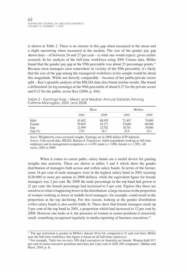
isshowninTable2.Thereisnoclosureinthisgapwhenmeasuredatthemeananda slight narrowingwhenmeasured at themedian. The size of the gender pay gapshownhere–ofbetween24and27percent–iswhatonewouldexpect,givenearlierresearch. Inhisanalysisof thefull-timeworkforceusing2001Censusdata,Millerfoundthatthegenderpaygapatthe95thpercentilewasabout23percentagepoints.11Becausemostmanagersearnsomewhereinvicinityofthe95thpercentile,it’slikelythatthesizeofthegapamongthemanagerialworkforceinhissamplewouldbeaboutthismagnitude.Whilenotdirectlycomparable–becauseofherpublic/privatesectorsplit–Kee’squantileanalysisoftheHILDAdataalsofoundsimilarresults.Shefoundadifferential(inlogearnings)atthe90thpercentileofabout0.27fortheprivatesectorand0.12forthepublicsectorKee(2006,p.416).
Table 2 - Earnings Gap - Mean and Median Annual Salaries Among Fulltime Managers, 2001 and 2008
Mean Median 2001 2008 2001 2008Male 81,602 88,955 72,407 79,000Female 59,603 65,173 53,666 60,000Gap 21,999 23,782 18,741 19,000Gap(%) 27.0 26.7 25.9 24.1
Notes:Weightedbycross-sectionalweights.Earningsarein2008dollars(CPIindexed).Source:Unitrecorddata,HILDA,Release8.Population:Adultrespondentsworkingasfull-timeemployeesandinmanagementoccupations,n=4,391(malen=3,006,femalen=1,385).Allwaves,2001to2008.
Whenitcomestocareerpaths,salarybandsareausefuldeviceforgaininginsights into seniority. These are shown in tables 3 and 4which show the genderdistributionofmanagersbothacrossandwithinsalarybands.Intermsoftheformer,some14percentofmalemanagerswereinthehighestsalarybandin2001(earning$120,000ormoreperannumin2008dollars),whiletheequivalentfigureforfemalemanagerswas2percent.By2008themalepercentageinthetopbandhadgrownto21percent;thefemalepercentagehadincreasedto5percent.Figureslikethesearesensitivetowhatishappeninglowerinthedistribution:alargeincreaseintheproportionofwomenworkingaslowerormiddlelevelmanagers,forexample,couldresultintheproportion at the top declining. For this reason, looking at the gender distributionwithinsalarybandsisalsouseful(table4).Theseshowthatfemalemanagersmadeup5percentofthetopbandin2001,aproportionwhichhadincreasedto12percentby2008.Howeveronelooksatit,thepresenceofwomeninseniorpositionsismassivelysmall,somethingrecognisedregularlyinmediareportingofbusinessexecutives.12
11TheagerestrictionisgreaterinMiller’sdataset20to64,comparedto21andoverhere;Millerusesthefull-timeworkforce,thisfigureisbasedonallfull-timeemployees.12Forexample,‘Onlytwoinevery100chiefexecutivesinAustraliaarefemale.Womenhold10.7percentofseniorexecutivepositionsandchairjust2percentofASX200companies’(MaharandHurst,2010,p.4).

63IAN WATSON
Decomposing the Gender Pay Gap in the Australian Managerial Labour Market
Table 3 - Distribution of Managers Across Salary Bands, 2001 and 2008 (Column %)
2001 2008 Male Female Total Male Female TotalUnder$40,000 10 22 14 8 18 12$40,000to$60,000 24 34 27 21 31 24$60,000to$80,000 25 25 25 22 26 23$80,000to$100,000 19 11 17 16 14 16$100,000to$120,000 8 6 7 11 6 9$120,000orover 14 2 10 21 5 16Total 100 100 100 100 100 100n 388 161 549 422 229 651
Notes:Weightedbycross-sectionalweights.Earningsarein2008dollars(CPIindexed).Source:Unitrecorddata,HILDA,Release8.Population:Adultrespondentsworkingasfull-timeemployeesandinmanagementoccupations,n=4,391(malen=3,006,femalen=1,385).Allwaves,2001to2008.
Table 4 - Distribution of Managers Within Salary Bands, 2001 and 2008 (Row %)
2001 2008 Male Female Total Male Female TotalUnder$40,000 10 22 14 8 18 12$40,000to$60,000 24 34 27 21 31 24$60,000to$80,000 25 25 25 22 26 23$80,000to$100,000 19 11 17 16 14 16$100,000to$120,000 8 6 7 11 6 9$120,000orover 14 2 10 21 5 16Total 100 100 100 100 100 100n 388 161 549 422 229 651
Notes:Weightedbycross-sectionalweights.Earningsarein2008dollars(CPIindexed).Source:Unitrecorddata,HILDA,Release8.Population:Adultrespondentsworkingasfull-timeemployeesandinmanagementoccupations,n=4,391(malen=3,006,femalen=1,385).Allwaves,2001to2008.
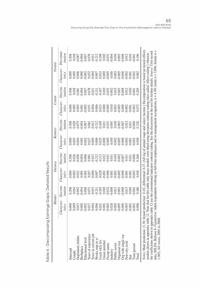
4. Results Decomposition Results Theextenttowhichdiscriminationaccountsforthegenderpaygapvariesbetween65percentand94percent,dependingontheapproachonetakes.ThehigherfigurecomesfromusingtheOaxacamethod,whilethelowerfigurecomesfromtheBlindermethod.Thesedecompositionresultsareshowninsummaryformintable5andwithamoredetailedbreakdownintable6.
This figure of 94 per cent represents 0.260 out of a total (log) earningsdifferentialof0.278.Theremaining.018ofthegapisduetodifferingcharacteristicsbetweenthesexes.Inthecaseofthe65percentfigure,thebreakdownis0.180fordiscrimination and 0.098 for characteristics (see the Oaxaca and Blinder rows intable5).Thegenderdifferences incoefficients,whenapplied to thecharacteristicsoffemalemanagers,showthatthegapispredominantlyclosedbyhoursworkedand

64AUSTRALIAN JOURNAL OF LABOUR ECONOMICSVOLUME 13 • NUMBER 1 • 2010
weeksworked(thesehavenegativesigns)(seetable6).Thedifferencesinreturnsonoccupationalstatusscorealsohelpsclosethegap.
Sowhatwidensthegap?Itispredominantlyyearsoflabourforceexperience,withpositivefiguresintherangeof0.071to0.091.Justaboutalloftheothervariableswithpositivesignshavequitesmallmagnitudes(lessthan0.015).Leavingasidelabourforceexperience(towhichIreturningreaterdetaillater),whydoestheunexplainedcomponentremainsolargewhenmostvariablesinthemodelhelptoclosethegenderdifferential? The answer lies in the intercept, a figure of considerable magnitude:0.508.Asnotedearlier,theinterceptrepresentsgroupmembership:itisthecomponentof thewage differentialwhich reflects being female rather thanmale. In the earlydecompositionstudies,itwasviewedasthemostblatantmeasureofdiscrimination(see,forexample,Blinder,1973).
Table 5 - Decomposing Earnings Gaps: Summary of Results
Differential due to: Discrimination Decomp into: Male Female Unexplained Characteristics Discrimination advantage disadvantage as %Blinder 0.098 0.180 0.000 0.180 64.8Oaxaca 0.018 0.260 0.260 0.000 93.5Reimers 0.058 0.220 0.130 0.090 79.1Cotton 0.073 0.205 0.082 0.123 73.8Pooled 0.082 0.196 0.099 0.097 70.5
Notes:Maleprediction:11.30;femaleprediction:11.02,differential:0.27.(Alllogofannualwageandsalaryincome.)Decompositionisbasedonofmixed-effectsmodelsshowninappendixtable12.Source:Unitrecorddata,HILDA,Release8. Population:Adultrespondentsworkingasfull-timeemployeesandinmanagementoccupations,n=4,391(malen=3,006,femalen=1,385).Allwaves,2001to2008.
Oneofthekeyadvantagestousingpaneldataforastudysuchasthisistheincreased precision of the estimates.Becausemanagers comprise such a relativelysmallsectionoftheworkforce,samplesizeconsiderationsbecomeparamountwhendrawinginferences.Inanalysingasinglewaveofdatathesamplesizeforbothmaleandfemalemanagerscanbeaslowas546.Ontheotherhand,usingalleightwavesofdataprovidesasamplesizeof4,391.13Validstatisticalinferencerequiressomemeasureofuncertaintyinthemodellingandthedecompositionapproachinthisarticleisnoexception.AsJann(2008,pp.458-460)argues,variabilityentersthedecompositionresultsthroughboththevariancesofthecoefficientsandtheuseofrandomvariablesfromsurveysampledata.Becausethedecompositionmethodentailedmultiplyingthecoefficientsandthemeansoftheserandomvariables,onemusttakeaccountofbothsourcesofvariation.FollowingSinninget al. (2008,pp.489-90),theapproachusedinthisstudyinvolvedbootstrappingtoobtainstandarderrorsforthefinaldecompositionresults.Thisapproachhasadvantageswhen thecomputationofanalytical standarderrorsiscomplex,andiswellsuitedtopaneldatamodelslikethoseemployedhere
13Ofcourse,manyoftheseobservationsarethesamepersonrepeatedandarenotindependentobservations.Thisisthemainreasonwhymixed-effectsmodellingisemployedintheanalysis.
65IAN WATSON
Decomposing the Gender Pay Gap in the Australian Managerial Labour Market
Tab
le 6
- D
ec
om
po
sin
g E
arn
ing
s G
ap
s: D
eta
iled
Re
sult
s
Bl
inde
r O
axac
a Re
imer
s Co
tton
Pool
ed
Char
acte
r- D
iscrim
- Ch
arac
ter-
Disc
rim-
Char
acte
r- D
iscrim
- Ch
arac
ter-
Disc
rim-
Char
acte
r- D
iscrim
in-
ist
ics
inat
ion
istic
s in
atio
n ist
ics
inat
ion
istic
s in
atio
n ist
ics
inat
ion
Intercept
0.000
0.508
0.000
0.508
0.000
0.508
0.000
0.508
0.000
0.508
Couple
0.009
0.014
-0.003
0.026
0.003
0.020
0.005
0.018
0.005
0.018
Dependentch
ildre
0.013
-0.092
-0.021
-0.058
-0.004
-0.075
0.003
-0.081
0.008
-0.087
Birth
place
0.000
-0.004
0.001
-0.004
0.001
-0.004
0.001
-0.004
0.000
-0.004
Educationallevel
-0.002
0.008
-0.001
0.006
-0.002
0.007
-0.002
0.007
-0.002
0.007
Yearso
fexperien
ce
0.037
0.071
0.017
0.091
0.027
0.081
0.031
0.078
0.032
0.076
Yearsincurre
ntjob
0.004
-0.01
10.006
-0.01
30.005
-0.01
20.004
-0.01
10.004
-0.01
1Weeksem
pinyr
0.006
-0.21
10.007
-0.21
20.006
-0.21
20.006
-0.21
10.007
-0.21
2Usualw
klyhrs
0.021
-0.10
50.028
-0.11
30.025
-0.10
90.023
-0.10
70.024
-0.10
8Un
ionmem
ber
0.001
0.010
-0.001
0.012
-0.000
0.011
0.000
0.010
0.000
0.010
Occupstatus
-0.005
-0.032
-0.006
-0.031
-0.005
-0.031
-0.005
-0.031
-0.005
-0.031
Industry
0.020
-0.008
0.001
0.011
0.010
0.001
0.014
-0.002
0.016
-0.004
Publicsecto
r0.005
0.013
-0.001
0.019
0.002
0.016
0.003
0.015
0.003
0.016
Organisatsize
-0.005
0.003
-0.005
0.002
-0.005
0.003
-0.005
0.003
-0.005
0.003
Orgwithsinglewp
0.000
-0.008
-0.000
-0.007
0.000
-0.007
0.000
-0.008
0.000
-0.008
Non-cityresid
-0.003
0.013
-0.001
0.011
-0.002
0.012
-0.002
0.012
-0.002
0.012
Stat
-0.001
0.010
-0.001
0.011
-0.001
0.011
-0.001
0.010
-0.001
0.010
Timep
eriod
-0.002
-0.001
-0.003
0.000
-0.002
-0.000
-0.002
-0.001
-0.002
-0.001
Total
0.098
0.180
0.018
0.260
0.058
0.220
0.073
0.205
0.082
0.196
Note
s:Malep
rediction:11
.30;femalep
rediction:11
.02,differential:0.27.(Alllogofan
nualwagea
ndsalaryincome.)Decom
positionisbasedonmixed-effe
cts
modelssh
owninap
pendixtable1
2.Notethatforthistableo
nlythosem
odelswerefi
ttedusingdeviationcontrastcoding(also
called`effectcoding’)wh
ereas
thec
oefficie
ntsshowninap
pendixtable1
2usetheco
nventionalindica
torcontrastcoding.Seethed
iscussio
ninthetextforfu
rtherdetails.S
ourc
e:Un
itrecord
data,H
ILDA
,Rele
ase8
.Pop
ulat
ion:Adultrespondentsw
orkingasfull-tim
eemployeesandinmanagem
entoccupations,n=4,391(malen
=3,006,femalen
=
1,385).Allwa
ves,2001to2008.

66AUSTRALIAN JOURNAL OF LABOUR ECONOMICSVOLUME 13 • NUMBER 1 • 2010
(CameronandTrivedi,2005,p.377).14Thisbootstrappingapproachsuggests that thegenderpaydifferentialhasa
standarderrorofabout0.02,givingaconfidenceintervalofbetween0.25and0.31(table7).Thefiguresreportedearlierintable5arealsoreproducedbelowintables8andtables9,withtheirstandarderrorsandconfidenceintervalsshownbesidethem.TheOaxacamethodsuggests that thediscriminatorycomponentof thegenderpaygapliesbetween80percentand106percent,whilsttheBlindermethodsuggestsanintervalofbetween51percentand72percent.
Table 7 - Confidence Intervals for Gender Pay Differential
Method Est SE LB UBPredictedmale 11.30 0.01 11.29 11.32Predictedfemale 11.02 0.01 11.00 11.05Differential 0.28 0.02 0.25 0.31
Notes:Est=estimate;SE=standarderror;LB=lowerconfidenceintervalbound;UB=upperbound.95percentconfidenceintervals.Basedonbootstrappingthemixed-effectsmodelsshownintable12butwithoutAR1correlationofresiduals.Thepredictedearningsareshownasthenaturallogofannualwageandsalaryincome,andthedifferentialisalsoonthisscaleSource:Unitrecorddata,HILDA,Release8.Population:Adultrespondentsworkingasfull-timeemployeesandinmanagementoccupations,n=4,391(malen=3,006,femalen=1,385).Allwaves,2001to2008.
Table 8 - Confidence Intervals for Discrimination as Percentage of Differential
Method Est SE LB UBBlinder 61.7 5.3 51.2 72.2Oaxaca 93.1 6.5 80.3 105.9Reimers 77.4 4.6 68.3 86.5Cotton 71.6 4.6 62.7 80.5Pooled 68.9 4.2 60.6 77.2
Notes:95percentconfidenceintervals.Basedonbootstrappingthemodelsshownintable12butwithoutAR1correlationofresidualshencethepointestimatesslightlydifferfromthoseshownintable5.Source:Unitrecorddata,HILDA,Release8.Population:Adultrespondentsworkingasfull-timeemployeesandinmanagementoccupations,n=4,391(malen=3,006,femalen=1,385).Allwaves,2001to2008.
14Bootstrapping,using2400repetitions,wascarriedoutforthemixed-effectsmodelsusingthebootfunction,(seeCantyandRipley,2009;andDavisonandHinkley,1997).Forefficiencythesnowpackagewasusedtoparallelisethebootstrapping,(seeTierney et al.,2009a;andTierneyet al.,2009b).TheAR1correlationusedforthemixed-effectsmodellinginthemaindecompositionresultscouldnotberepeatedinthebootstrap,becauseanyrepetitionofanobservationfromthesameyear violated theAR1 assumption. For this reason the point estimates in the confidenceintervalsdifferfromthoseinthemaindecompositionresults.

67IAN WATSON
Decomposing the Gender Pay Gap in the Australian Managerial Labour Market
Table 9 - Confidence Intervals for Characteristics and Discrimination Components
Characteristics DiscriminationMethod Est SE LB UB Est SE LB UBBlinder 0.108 0.017 0.074 0.141 0.173 0.016 0.142 0.205Oaxaca 0.019 0.019 -0.017 0.056 0.262 0.019 0.224 0.299Reimers 0.064 0.014 0.035 0.092 0.218 0.014 0.190 0.245Cotton 0.080 0.015 0.051 0.108 0.201 0.014 0.174 0.228Pooled 0.087 0.014 0.060 0.115 0.194 0.013 0.168 0.220
Notes:95percentconfidenceintervals.Basedonbootstrappingthemodelsshownintable12butwithoutAR1correlationofresiduals.Source:Unitrecorddata,HILDA,Release8.Population:Adultrespondentsworkingasfull-timeemployeesandinmanagementoccupations,n=4,391(malen=3,006,femalen=1,385).Allwaves,2001to2008.
Simulated Change Results IntheOlsen-Walbyapproach,theemphasisisonsimulatedchange,anditsconsequencesforclosingthegenderpaygap.Byhypothesisingvariouschanges–someofwhichmayhavepolicyrelevance–onecanestimatehowmuchthegapwouldcloseinpercentageterms,andhowmuchthiswouldbeworthtowomenindollarterms.
Table 10 shows the simulated change results for the pooled version of themixed-effectsmodelandhighlights thekeyfindingthatgroupmembership, that is,simply being female, counts for $12,899 of the $18,400 pay gap.15 This representsabout70percentoftheoverallpaygap.Someoftheindividualcomponentsarealsorevealing.Less labourforceexperience iscostlyforfemalemanagers:weretheytomatchmalemanagersinthisrespecttheywouldbeearninganadditional$2,153perannum.Iftheirfamilylife–coupleandchildrenvariables–werealsorewardedinthesameway,womenmanagerswouldbeearningabout$870moreperannum.Andifwomenmanagerscouldmatchthehoursroutinewhichmalemanagersmaintain,thatwouldbeworthanadditional$1,607perannum.Thesekeyareas–whichreflecttheinterfacebetweenworkplaceandfamilylife–arethemajorelementsinthegenderpaygapusingthissimulatedchangeapproach.Mostoftheothervariablesshoweithertrivialamountsoramountswhichfavourwomen.Clearly,labourforceexperienceandfamilylifewarrantcloserinspect.
15Notethatthegaphereisnotbasedonweightedfigures,butcomesfromtheunweightedmodellingdata.

68AUSTRALIAN JOURNAL OF LABOUR ECONOMICSVOLUME 13 • NUMBER 1 • 2010
Table 10 - Olsen-Walby Simulated Change: Detailed Results
∆X b b9∆X Simul Male Female Change Overall Simul chng as Ann $ avg avg factor coef effect % gap equivalFemale 0.000 1.000 -1.000 -0.192 0.192 0.701 12,899Couple 0.825 0.679 0.146 0.036 0.005 0.019 349Onedepchild 0.173 0.168 0.005 0.001 0.000 0.000 0Twodepchild 0.212 0.092 0.120 0.032 0.004 0.014 255Three+depchild 0.081 0.017 0.064 0.061 0.004 0.014 266BornEngspkcountry 0.140 0.103 0.037 0.010 0.000 0.001 25BornNon-Engspk 0.085 0.087 -0.001 -0.057 0.000 0.000 6Vocationalquals 0.332 0.258 0.074 -0.261 -0.019 -0.071 -1,303Year12quals 0.129 0.157 -0.028 -0.224 0.006 0.023 421Year11orbelow 0.127 0.157 -0.031 -0.378 0.012 0.042 780Yearsofexperience* 22.951 19.830 3.121 0.053 0.032 0.117 2,153Jobtenure 8.606 7.128 1.478 0.003 0.004 0.016 287Weeksemployedinyr 51.615 51.183 0.431 0.015 0.007 0.024 440Usualwklyhrs 48.527 45.215 3.311 0.007 0.024 0.087 1,607Unionmember 0.193 0.253 -0.060 -0.004 0.000 0.001 17Occupstatus 65.008 66.371 -1.363 0.004 -0.005 -0.020 -366Primaryindustry 0.075 0.013 0.062 -0.014 -0.001 -0.003 -57Construct/utilities 0.066 0.014 0.052 0.054 0.003 0.010 192Wholesale/transport 0.101 0.040 0.061 0.010 0.001 0.002 39Retail 0.099 0.157 -0.058 -0.064 0.004 0.013 247Accommodation,cafesetc 0.056 0.073 -0.017 -0.156 0.003 0.010 183Informationservices 0.035 0.030 0.006 0.082 0.000 0.002 31Finance&insurance 0.073 0.075 -0.002 0.109 -0.000 -0.001 -16Businessservices 0.090 0.133 -0.043 0.070 -0.003 -0.011 -200Government 0.110 0.113 -0.002 0.036 -0.000 -0.000 -5Education 0.068 0.105 -0.038 -0.038 0.001 0.005 97Health&community 0.026 0.144 -0.117 -0.070 0.008 0.030 550Otherservices 0.038 0.049 -0.011 -0.044 0.000 0.002 33Publicsector 0.196 0.290 -0.094 -0.028 0.003 0.009 174Orgsize:20-99 0.172 0.159 0.013 0.095 0.001 0.005 84Orgsize:100-499 0.184 0.178 0.006 0.149 0.001 0.003 64Orgsize:500plus 0.485 0.529 -0.043 0.170 -0.007 -0.027 -496Orgwithsinglewp 0.239 0.232 0.007 0.011 0.000 0.000 6Non-cityresid 0.330 0.309 0.021 -0.100 -0.002 -0.008 -143Vic 0.261 0.242 0.019 -0.050 -0.001 -0.004 -65Qld 0.182 0.210 -0.028 -0.066 0.002 0.007 123SA,Tas 0.097 0.078 0.019 -0.108 -0.002 -0.007 -137WA&NT 0.091 0.092 -0.000 -0.054 0.000 0.000 1ACT 0.040 0.042 -0.002 -0.013 0.000 0.000 2Year:2002 0.126 0.118 0.008 0.118 0.001 0.004 67Year:2003 0.125 0.119 0.006 0.189 0.001 0.004 76Year:2004 0.128 0.128 0.000 0.303 0.000 0.000 6Year:2005 0.116 0.118 -0.002 0.413 -0.001 -0.002 -44Year:2006 0.127 0.123 0.004 0.096 0.000 0.002 28Year:2007 0.118 0.129 -0.011 0.130 -0.001 -0.005 -100Year:2008 0.131 0.151 -0.019 0.130 -0.003 -0.009 -171Intercept 1.000 1.000 0.000 9.240 0.000 0.000 0Totals 0.274 1.000 18,400
Notes:Basedonthepooledmodelshownintable12.*Exceptforthemaleandfemaleaverages,thelabourforceexperiencefiguresshownhererepresentthesummationofeachoftheregressors(thatis,experience,experiencesquaredandexperiencecubed).Source:Unitrecorddata,HILDA,Release8.Population:Adultrespondentsworkingasfull-timeemployeesandinmanagementoccupations,n=4,391(malen=3,006,femalen=1,385).Allwaves,2001to2008.

69IAN WATSON
Decomposing the Gender Pay Gap in the Australian Managerial Labour Market
5. DiscussionDirect Discrimination The results discussed in the last section are reasonablyunambiguous, though theirinterpretationmaybelessso.Womenfull-timemanagersearnabout27percentlessthantheirmalecounterpartsandsomewherebetween65and90percentofthispaygap cannot be explained by the characteristics ofmanagers and is possibly due todiscrimination.Indeed,thecharacteristicsofmaleandfemalemanagers–atleastasmeasuredinthissample–areremarkablysimilar.Oneisleftwiththestarkconclusionthatthemajorpartofthegapissimplyduetowomenmanagersbeingfemale.
Despitequitedifferentmethodologicalapproaches,theseresultsareconsistentwiththefindingsofBarónandCobb-Clark(2008), thestudymostsimilarinscopeto this one.While their results are presented separately for the public and privatesectors,therangeofestimatesfortheunexplained(discriminatory)componentoftheirdecompositionisquitesimilartotheseresults.Theyfind,forexample,thatthepublicsectorfigureis92percentwhenoccupationisexcluded,and88percentwhenitisincluded.Fortheprivatesector,thecomparablefiguresare59percentand52percent.Onewouldassumethatweretheseresultspooled,thentheall-sectoraverageswouldliesquarelywithinthe65to90percentrangefoundinthisstudy.
The management literature which deals with the glass ceiling providesqualitativeinsightsintohowdiscriminationmayoperateatseniorlevelsofmanagement(Sinclair,2005).Ithasbeenargued,forexample,thatwomen’smovementintoseniormanagementjobscanbeblockedby‘exclusionarymasculinepractices’(Sinclair,1994).Aswithmany in-groups,suchpractices include therecruitmentof ‘similar’personsintohigherpositions.This‘cloningeffect’,alsotermeda‘mateshipthing’ora‘comfortthing’,canrestricttherangeofpeoplewhoendupbeingrecruitedorpromoted:
Manymanagersfavourcandidateswhoappeartobelikethemselves.Itmakesthemfeelthattheyunderstandthepersonandcantrusthimorher.Theyoftenusewordslikecomfort,fit,andteamtoexpressthatdesire...Thosearecodewordsforthe‘ingroup’,the‘club’,orthe‘oldboys’network’(JeffalynJohnson,citedinGentile,1991,pp.22).
At its crudest, this reduces to ‘Men employ men’: ‘Male executives support andpromoteothermenlookinglikethemselvesandtheyuseeachotherssuccesstotheirownadvantage’(Lausten,2001,p.3).
Evenwhen theculturalnormsarenot thisblatant,gender-stereotypingcanstillplayitspartinlimitingwomen’sadvancement:‘thetendencytochoosemenmay...reflectatendencytodefineleadershipintermsoftask-orientedcontributions’(EaglyandKarau, cited inBeyer, 2007,p. 487).This insight ispartof abroader analysiswhicharguesthatthereisaninherentgenderbiasintheevaluationofmenandwomenintheworkplace,with‘greatersocialsignificanceandgeneralcompetenceattributedtomenoverwomen’(Beyer,2007,p.494;andseealsoChung,2001).
Quantitativeevidenceonpromotionsandearningssuggeststhattheproblemisindeedacomplexone.Arecentstudyonpromotions(Boothet al.,2003)usingtheBritishHouseholdPanelSurveyfoundevidencethatwomenwerejustaslikelytobepromoted asmen, but that the pay increases they received from those promotionsweresmaller.Thesefindingswereconsistentwithasticky-floorsmodelofpromotion:

70AUSTRALIAN JOURNAL OF LABOUR ECONOMICSVOLUME 13 • NUMBER 1 • 2010
‘themechanismsoperatingarenotthesimpleglassceilingsonesofanunfavourablepromotionsrateforwomen,butinvolvelowerwagereturnstopromotionforwomen’(2003,p.297).Theimplicationsofthisforthepresentstudyaresubtle,butimportant:‘thepromotionprocess...mayverywellincreasethedisadvantage,notthroughalowerpromotion probability, but through a lower wage reward over time to promotion’(2003,p.319).Inotherwords,theassumptionofasimplelinkbetweenpayequityandsenioritymaybeinadequate.Womenmaybeclimbingthecorporateladderatasimilarratetomen,butstillslippingbehindontheearningsladder,therebyleavingthegenderpaygap largelyundisturbed.Boothet al. (2003,p.319) sumup these implicationswell: ‘Women do not catch up onmen from the promotions process, and the paydifferentialmaywidenasbothmenandwomenarepromoted.Theimplicationisthatitisnotsufficientforpolicypurposestoensureequalopportunitiesinpromotions.Itisnecessaryaswelltolookatissuesofpaywithinrank...’
Is there evidence for this in Australia? The HILDA survey also askedrespondents (from 2002 onwards) about whether they had received promotions inthepreviousyear.Among the sampleofmanagersused in this study, somesimpledescriptivetables(notshown)partlyendorsetheBoothet al.(2003)findings.Femalemanagerswere no less likely thanmalemanagers to gain a promotion during theyear, and this also applied in the top salary bands.Moreover, the annual increasein earnings for those promotedwere roughly equivalent betweenmale and femalemanagers.16TheBoothet al.(2003)studywasestimatedforthesampleasawhole,ratherthanjustmanagers–asinthisstudy–soitsdirectrelevanceforthemanageriallabourmarketmaybelimited.Theirstudydid,however,entailamultivariateanalysis,soitsfindingsaremorerobustthansimpledescriptivetablesfromtheHILDAdata.Clearly,studieslikethosebyBoothet al. (2003)emphasisetheneedformorenuancedaccountsofthecomplexitiesaroundrecruitment,promotions,seniorityandpayequity.
Indirect Discrimination Thefindingsfromthisstudyalsothrowlightontheinterfacebetweenfamilylifeandworkinglifeanditsimplicationsforwomen’scareeradvancement.Theliteratureontheglassceilinghassuggestedthatmanagerialcareerpathsareinherentlygenderedwithanearlyinsightbeingthatseniormanagers‘treatallworkersasiftheyaremen’.Insodoing,theyfailtoprovidesupportfortheirstaffintheformofchildcare,parentalleaveorflexibleworkschedules(Newman,1993).Whatmakesthisdiscriminatoryinits impact is theprevailingdomestic divisionof labour,which leavesmostwomenwiththegreatershareofparentingandhousekeepingtasks(see,forexample,Bittmanand Lovejoy, 1993; and Baxter et al., 2005; andNoonan, 2001). The results fromthisstudy,particularlyaroundhoursofwork,labourforceexperienceandparentingreinforcethesearguments.Thenumberofhoursworkedareoneofthekeydifferencesbetweenmaleandfemalemanagers–bothofwhomareworkingfull-time–withtheformerdoing3.3hoursmoreperweekthanthelatter.Thisdoesnotnecessarilymeanthat femalemanagers, on average, achieved less. Ifwe assume that earnings relatetoproductivity tosomedegree, then thehigher returnonhoursworkedforwomen(shownbytheregressioncoefficients)meansthattheymaybejustasproductive,as16Thetablesarenotshownherebutareavailablefromtheauthor.

71IAN WATSON
Decomposing the Gender Pay Gap in the Australian Managerial Labour Market
agroup,despiteworkingfewerhours.Similarly,yearsoflabourforceexperienceisalsoanareawherethemaleandfemalepopulationsdiffer:malemanagershave,onaverage,3.2moreyearsoflabourforceexperience.However,theirrespectivereturnsonexperiencedifferconsiderablytowardsthelatteryearsofworkinglife,theperiodwhen seniority is usually achieved.Aglass ceiling is evident in theway inwhichlonger years of experience no longer count for as much among female managerswhenitcomestoreturnsonexperience.Finally,thepresenceofdependentchildrenalsomakesadifference,evidentintheregressioncoefficients(table12)whichshowincreasinglynegativereturnsforeachadditionalchild,particularlythethird.
In practice, these factors – hoursworked, labour force experience and thepresenceofchildren–combineinsuchawaythattheearningsoffemalemanagersfallwell behind those ofmalemanagers, evenwhen their other characteristics areequivalent.Thiscanbeseenquiteclearlyinearningspredictionsfromtheregressionmodelling,inwhichreturnsonlabourforceexperienceareconditionedonthepresenceofchildren.Thesepredictionstaketheaveragecharacteristicsofthepooledsample–thatis,theaveragesforbothmalesandfemales–andapplytherespectivemaleandfemaleregressioncoefficients.Theresultsareshowninfigures1and2.Thegraphdataisthesameinboth,buteachpresentationemphasisesadifferentfacet.Infigure1themaleandfemalelinesareoffsetlargelybythedifferenceinintercepts(thegroupmembershipcomponent)andcanbeoverlookedforthepurposesofthisillustration.Interestcentresonthetrajectoryofthelinesandtheinfluenceofchildren.Lookingatthefirstpanel,wheretherearenodependentchildreninthepicture,thegraphshowsthatthereturnsonlabourforceexperiencearethesameformenandwomenintheearlyyears,butthenplateauanddeclineatquitedifferentrates.Formalemanagers,theiryearsofexperiencecontinuetoprovideareturnrightthroughtheirworkinglives(thoughatadiminishingrateofincrease).Bycontrast,forfemalemanagerstherateofreturnbeginstosteadilydeclineafterabouttwentyyears.Eachsuccessivepanelinfigure1showshowtheadditionofchildrenservestowidenthegapbetweenmenandwomen,andthisappliesintheearlyyearsaswellastowardstheend.Theeffectofchildrenisalsohighlightedinfigure2wheretheadditionofeachdependentchildraises the line formen,but shifts itdownwards forwomen,with themostdecisivedropsoccurringforthefirstchildandthethird.
These results are also consistentwith the qualitative findings on the glassceilingwhich emphasises how gender arrangements shape the prospects of careeradvancement. These are the various ways in which gender discrimination worksindirectly.Thelongerhoursofworkputinbymalemanagers–whichmakesthemmorevisibleintheworkplace–ismadepossiblebythedomesticdivisionoflabourwherebythebulkofparentingresponsibilitiesfallonwomen.Similarly,suchdomesticarrangements provide an opportunity formalemanagers to travel as part of theirworkinwayswhichareoftenimpossibleorimpracticalforfemalemanagers.Finally,the unbroken years of labour force experience bymen can alsowork in favour ofmanagerialcareerpaths, signallinga levelof ‘commitment’whichmaybedeemedmissingamongfemalemanagerswhohavetakentimeoutforparenting.

72AUSTRALIAN JOURNAL OF LABOUR ECONOMICSVOLUME 13 • NUMBER 1 • 2010
Figure 1 - Predicted Earnings by Years of Experience, Number of Children and Sex
Source:Maleandfemalemodelsshownintable12.
Figure 2 - Predicted Earnings by Years of Experience, Sex and Number of Children
Source:Maleandfemalemodelsshownintable12.
Three or moreTwo
120
60
100
80
None One
120
30
60
2010
100
80
40 302010 40
Pred
icte
d ea
rnin
gs $
’000
s
Years of experience
SexMale Female
FemaleMale
120
30
60
2010
100
80
40 302010 40
Pred
icte
d ea
rnin
gs $
’000
s
Years of experience
Number of childrenNone One Two Three or more

73IAN WATSON
Decomposing the Gender Pay Gap in the Australian Managerial Labour Market
Inconclusion,theinterceptterm–groupmembership–accountsforthevastmajorityofthediscriminatorycomponentinthegenderpaygap.Atthesametime,thoseaspectsofworkinglifewhichintersectmostprofoundlywithfamilylife–hoursworked,thepresenceofchildrenandyearsoflabourforceexperience–arealsothevariablesintheseregressionmodelswhichappeartowidenthegapmostdramatically.Howeveronelooksatit,theevidencepointstowardsbothdirectandindirectdiscriminationasmajorobstaclesinachievinggenderequityinthemanageriallabourmarket.
Appendix A
Table A.1 - Summary Statistics for Sample in Models
Means/percentage Standard deviations Male Female All Male Female AllSingle 17.5 32.1 22.1Couple 82.5 67.9 77.9Nochildren 53.5 72.4 59.4Onedepchild 17.3 16.8 17.1Twodepchild 21.2 9.2 17.4Three+depchild 8.1 1.7 6.1BornAustralia 77.5 81.1 78.6BornEngspkcountry 14.0 10.3 12.8BornNon-Engspk 8.5 8.7 8.6Universityquals 41.3 42.8 41.7Vocationalquals 33.2 25.8 30.9Year12quals 12.9 15.7 13.8Year11orbelow 12.7 15.7 13.6Yearsofexperience 23.0 19.8 22.0 11.0 10.3 10.9Jobtenure 8.6 7.1 8.1 8.5 7.9 8.4Weeksemployedinyr 51.6 51.2 51.5 2.5 4.0 3.0Usualwklyhrs 48.5 45.2 47.5 7.4 7.2 7.5Notunionmember 80.7 74.7 78.8Unionmember 19.3 25.3 21.2Occupstatus 65.0 66.4 65.4 14.7 15.6 15.0Manufacturing 16.3 5.5 12.9Primaryindustry 7.5 1.3 5.6Construct/utilities 6.6 1.4 5.0Wholesale/transport 10.1 4.0 8.2Retail 9.9 15.7 11.7Accommodation,cafesetc 5.6 7.3 6.1Informationservices 3.5 3.0 3.3Finance&insurance 7.3 7.5 7.4Businessservices 9.0 13.3 10.4Government 11.0 11.3 11.1Education 6.8 10.5 7.9Health&community 2.6 14.4 6.3Otherservices 3.8 4.9 4.1Privatesector 80.4 71.0 77.5Publicsector 19.6 29.0 22.5Orgsize:under20 15.9 13.5 15.1Orgsize:20-99 17.2 15.9 16.8Orgsize:100-499 18.4 17.8 18.2Orgsize:500plus 48.5 52.9 49.9Orgwithmultiplewps 76.1 76.8 76.3

74AUSTRALIAN JOURNAL OF LABOUR ECONOMICSVOLUME 13 • NUMBER 1 • 2010
Table A.1 - Summary Statistics for Sample in Models (continued)
Means/percentage Standard deviations Male Female All Male Female AllOrgwithsinglewp 23.9 23.2 23.7Cityresident 67.0 69.1 67.6Non-cityresid 33.0 30.9 32.4NSW 32.8 33.6 33.1Vic 26.1 24.2 25.5Qld 18.2 21.0 19.1SA,Tas 9.7 7.8 9.1WA&NT 9.1 9.2 9.2ACT 4.0 4.2 4.1Year:2001 12.8 11.5 12.4Year:2002 12.6 11.8 12.3Year:2003 12.5 11.9 12.3Year:2004 12.8 12.8 12.8Year:2005 11.6 11.8 11.7Year:2006 12.7 12.3 12.6Year:2007 11.8 12.9 12.1Year:2008 13.1 15.1 13.8Male 68.5Female 31.5
Note:Allwaves(2001to2008).Source:Unitrecorddata,HILDA,Release8.Population:Adultrespondentsworkingasfull-timeemployeesandinmanagementoccupations,n=4,391(malen=3,006,femalen=1,385).Allwaves,2001to2008.
Table A.2 - Models Used for Decomposition: Coefficients and Standard Errors
Male Female Pooled Coef SE Coef SE Coef SEIntercept 9.418 (0.128) 8.882 (0.142) 9.240 (0.093)Couple 0.063 (0.021) -0.018 (0.022) 0.036 (0.015)Onedepchild 0.024 (0.018) -0.065 (0.024) 0.001 (0.015)Twodepchild 0.061 (0.022) -0.071 (0.033) 0.032 (0.018)Three+depchild 0.093 (0.030) -0.181 (0.071) 0.061 (0.027)BornEngspkcountry 0.010 (0.033) 0.023 (0.043) 0.010 (0.026)BornNon-Engspk -0.036 (0.038) -0.062 (0.046) -0.057 (0.030)Vocationalquals -0.275 (0.025) -0.220 (0.033) -0.261 (0.020)Year12quals -0.207 (0.033) -0.222 (0.039) -0.224 (0.026)Year11orbelow -0.402 (0.035) -0.301 (0.041) -0.378 (0.027)Yearsofexperience 0.053 (0.009) 0.055 (0.011) 0.054 (0.007)Yearsofexperiencesquared -0.001 (0.000) -0.002 (0.001) -0.002 (0.000)Yearsofexperiencecubed 0.000 (0.000) 0.000 (0.000) 0.000 (0.000)Jobtenure 0.002 (0.001) 0.004 (0.002) 0.003 (0.001)Weeksemployedinyr 0.013 (0.002) 0.017 (0.002) 0.015 (0.001)Usualwklyhrs 0.006 (0.001) 0.009 (0.001) 0.007 (0.001)Unionmember -0.016 (0.019) 0.022 (0.025) -0.004 (0.015)Occupstatus 0.004 (0.001) 0.004 (0.001) 0.004 (0.000)Primaryindustry 0.004 (0.036) -0.101 (0.091) -0.014 (0.033)Construct/utilities 0.034 (0.031) 0.142 (0.079) 0.054 (0.029)Wholesale/transport 0.007 (0.024) 0.045 (0.056) 0.010 (0.022)

75IAN WATSON
Decomposing the Gender Pay Gap in the Australian Managerial Labour Market
Table A.2 - Models Used for Decomposition: Coefficients and Standard Errors (continued)
Male Female Pooled Coef SE Coef SE Coef SERetail -0.047 (0.029) -0.066 (0.052) -0.064 (0.025)Accommodation,cafesetc -0.185 (0.043) -0.103 (0.060) -0.156 (0.034)Informationservices 0.058 (0.042) 0.138 (0.063) 0.082 (0.035)Finance&insurance 0.145 (0.037) 0.046 (0.057) 0.109 (0.030)Businessservices 0.042 (0.027) 0.149 (0.047) 0.070 (0.023)Government 0.026 (0.035) 0.094 (0.057) 0.036 (0.029)Education -0.050 (0.043) 0.038 (0.059) -0.038 (0.034)Health&community -0.093 (0.049) 0.008 (0.054) -0.070 (0.033)Otherservices -0.062 (0.038) 0.032 (0.059) -0.044 (0.031)Publicsector -0.056 (0.027) 0.008 (0.032) -0.028 (0.021)Orgsize:20-99 0.110 (0.022) 0.047 (0.033) 0.095 (0.018)Orgsize:100-499 0.155 (0.025) 0.133 (0.036) 0.149 (0.021)Orgsize:500plus 0.179 (0.026) 0.142 (0.037) 0.170 (0.021)Orgwithsinglewp 0.020 (0.018) -0.008 (0.026) 0.011 (0.015)Non-cityresid -0.120 (0.022) -0.054 (0.029) -0.100 (0.018)Vic -0.071 (0.027) -0.016 (0.033) -0.050 (0.021)Qld -0.085 (0.029) -0.034 (0.036) -0.066 (0.023)SA,Tas -0.116 (0.039) -0.107 (0.052) -0.108 (0.031)WA&NT -0.067 (0.037) -0.011 (0.046) -0.054 (0.029)ACT -0.038 (0.054) 0.055 (0.064) -0.013 (0.042)Year:2002 0.110 (0.015) 0.138 (0.024) 0.118 (0.012)Year:2003 0.185 (0.017) 0.202 (0.026) 0.189 (0.014)Year:2004 0.299 (0.018) 0.313 (0.026) 0.303 (0.015)Year:2005 0.394 (0.019) 0.449 (0.027) 0.413 (0.016)Year:2006 0.083 (0.020) 0.119 (0.028) 0.096 (0.016)Year:2007 0.108 (0.020) 0.178 (0.028) 0.130 (0.016)Year:2008 0.110 (0.021) 0.176 (0.028) 0.130 (0.017)Female-0.192(0.019)StatisticsNulllog-likelihood -1182.1 -594.0 -1841.9Modellog-likelihood -648.4 -305.9 -876.6Randomeffects(SD) 0.30 0.27 0.30Sigma(SD) 0.25 0.21 0.24Rho 0.56 0.30 0.49N 3,006 1,385 4,391
Notes:Linearmixed-effectsmodelfittedbyREMLwithresidualcorrelationmodelledasAR1.Outcome variable:Logofannualwageandincomesalaryin2008dollars(CPIindexed).Standarderrorsinbrackets.Omittedcategoriesare:Single;Nochildren;BorninAustralia,Universityqualifications;Manufacturing;Privatesector,Orgsizeunder20;Orgwithmultiplewps;Cityresident;NSW;Male.Source:Unitrecorddata,HILDA,Release8.Population:Adultrespondentsworkingasfull-timeemployeesandinmanagementoccupations,n=4,391(malen=3,006,femalen=1,385).Allwaves,2001to2008.

76AUSTRALIAN JOURNAL OF LABOUR ECONOMICSVOLUME 13 • NUMBER 1 • 2010
References Albrecht,J.,Björklund,A.andVroman,S.(2003),‘IsThereaGlassCeilinginSweden’,
Journal of Labor Economics,21,145-177.Arulampalam,W.,Booth,A.L.andBryan,M.L.(2007),‘IsThereaGlassCeiling
overEurope?ExploringtheGenderPayGapacrosstheWageDistribution’,Industrial and Labor Relations Review,60,163-186.
Barón, J.D. and Cobb-Clark, D.A. (2008), Occupational Segregation and the Gender Wage Gap in Private-and Public-Sector Employment: A DistributionalAnalysis,DiscussionPaperNo.3562,Bonn:IZA–InstitutefortheStudyofLabor.
Bates, D. and Maechler, M. (2009), lme4: Linear mixed-effects models using S4 classes, R package version0.999375-32, URL: http://CRAN.Rproject.org/package=lme4.
Baxter,J.,Hewitt,B.andWestern,M.(2005),‘Post-FamilialFamiliesandtheDomesticDivision of Labor: A View from Australia’, The Journal of Comparative Family Studies,60,6-11.
Beblo,M.andWolf,E.(2002),Wage Penalties for Career Interruptions: An Empirical Analysis for West Germany,DiscussionPaperNo.02-45,Mannheim:ZEW–CentreforEuropeanEconomicResearch.
Becker, G. (1971), The Economics of Discrimination, Second, Chicago UniversityPress,Chicago.
Beyer,B.(2007),‘Twentyyearslater:explainingthepersistenceoftheglassceilingforwomenleaders’,Women in Management Review,22,482-496.
Bittman,M.andLovejoy,F.(1993),‘DomesticPower:NegotiatinganUnequalDivisionof Labourwithin a Framework of Equality’,Australian and New Zealand Journal of Sociology,29,302-321.
Blinder,A.S.(1973),‘WageDiscrimination:ReducedFormandStructuralEstimates’,Journal of Human Resources,18,436-455.
Bloom,D.andKillingsworth,M.(1982),‘PayDiscriminationResearchandLitigation:TheUseofRegression’,Industrial Relations,21,318-39.
Booth,A.L.,Francesconi,M.andFrank,J.(2003),‘Astickyfloorsmodelofpromotion,pay,andgender’,European Economic Review,47,295-322.
Borland, J. (1999), ‘TheEqualPayCase–ThirtyYearsOn’,Australian Economic Review,32,265-72.
Buchinsky,M.(1998),‘RecentAdvancesinQuantileRegressionModels’,The Journal of Human Resources,33,88-126.
Cameron, A.C. and Trivedi, P.K. (2005), Microeconometrics: Methods and Applications,CambridgeUniversityPress.
Canty,A. andRipley,B. (2009),boot: Bootstrap R (S-Plus) Functions,R packageversion1.2-36.
Chung,J.(2001),‘TheEffectsofRaterSexandRateeSexonManagerialPerformanceEvaluation’,Australian Journal of Management,26,147-163.
Cotton, J. (1988), ‘On the Decomposition of Wage Differentials’, The Review of Economics and Statistics,70,236-243.
Davison, A. and Hinkley, D. (1997), Bootstrap Methods and their Application,CambridgeUniversityPress,NewYork.

77IAN WATSON
Decomposing the Gender Pay Gap in the Australian Managerial Labour Market
DiNardo, J., Fortin, N.M. and Lemieux, T. (1996), ‘Labor Market Institutionsand the Distribution of Wages, 1973-1992: A Semiparametric Approach’,Econometrica,64,1001-1044.
Dolton, P.J. and Makepeace, G.H. (1986), ‘Sample Selection and Male-FemaleEarnings Differentials in the Graduate LabourMarket’,Oxford Economic Papers,38,317-341.
Gardeazabal, J. and Ugidos, A. (2004), ‘More on Identification in DetailedWageDecompositions’,Review of Economic and Statistics,86,1034-1036.
Gardeazabal,J.andUgidos,A.(2005),‘GenderWageDiscriminationatQuantiles’,Journal of Population Economics,18,165-179.
Gelman, A. and Hill, J. (2007),Data Analysis Using Regression and Multilevel/Hierarchical Models,CambridgeUniversityPress,Cambridge.
Gentile,M.(1991),‘TheCaseoftheUnequalOpportunity’,Harvard Business Review,69,14-25.
Gregory, R. and Duncan, R. (1981), ‘Segmented LabourMarket Theories and theAustralianExperienceofEqualPayforWomen’,Journal of Post-Keynesian Economics,403-28.
Heckman,J.J.(1979),‘SampleSelectionBiasasaSpecificationError’,Econometrica,47,153-161.
Holst,E.andBusch,A.(2009),Glass Ceiling Effect and Earnings – The Gender Pay Gap in Managerial Positions in Germany,SOEPpapersonMultidisciplinaryPanelDataResearchNo.201,Berlin:DIW.
Jann,B. (2008), ‘TheBlinder-Oaxaca decomposition for linear regressionmodels’,The Stata Journal,8,453-479.
Jones, F.L. and Kelley, J. (1984), ‘Decomposing Differences between Groups: ACautionaryNote onMeasuringDiscrimination’,Sociological Methods and Research,12,323-43.
Juhn,C.,Murphy,K.andPierce,B.(1991),‘Accountingfor theslowdowninblack-white wage convergence’, Workers and Their Wages: Changing Patterns in the United States, (ed.) by M. Kosters, American Enterprise Institute,Washington.
Kee,H.J.(2006),‘GlassCeilingorStickyFloor?ExploringtheAustralianGenderPayGap’,The Economic Record,82,408-427.
Koenker,R.andHallock,K.F.(2001),‘QuantileRegression’,The Journal of Economic Perspectives,15,143-156.
Lausten,M. (2001),Gender Differences in Managerial Compensation – Evidence from Denmark,WorkingPaper01-4,AarhusSchoolofBusiness,DepartmentofEconomics,UniversityofAarhus,URL:http://www.hha.dk/nat/WPER/01-4_ml.pdf.
Mahar,J.andHurst,D.(2010),‘PlantoMentorFemaleExecutives’,Sydney Morning Herald Business Day,1April2010.
Miller, P.W. (1994), ‘Occupational segregation andwages inAustralia’, EconomicsLetters,45,367-371.
Miller,P.W.(2005),‘TheRoleofGenderamongLow-PaidandHigh-PaidWorkers’,The Australian Economic Review,38,405-17.
78AUSTRALIAN JOURNAL OF LABOUR ECONOMICSVOLUME 13 • NUMBER 1 • 2010
Neuman,S.andOaxaca,R.L.(2004),‘Wagedecompositionswithselectivity-correctedwageequations:Amethodologicalnote’,Journal of Economic Inequality,2,3-10.
Neumark,D. (1988), ‘Employers’DiscriminatoryBehaviour and the Estimation ofWageDiscrimination’,Journal of Human Resources,23,279-295.
Newman, M. (1993), ‘Career Advancement: Does Gender Make a Difference?’,American Review of Public Administration,23,361-384.
Noonan,M.C.(2001),‘TheImpactofDomesticWorkonMen’sandWomen’sWages’,Journal of Marriage and Family,63,1134-1145.
Oaxaca,R.L.andRansom,M.R.(1994),‘Ondiscriminationandthedecompositionofwagedifferentials’,Journal of Econometrics,61,5-21.
Oaxaca, R.L. and Ransom, M.R. (1999), ‘Identification in Detailed WageDecompositions’,The Review of Economics and Statistics,81,154-157.
Oaxaca, R. (1973), ‘Male-Female Wage Differentials in Urban Labor Markets’,International Economic Review,14,693-709.
Olsen,W.andWalby,S.(2004),Modelling Gender Pay Gaps,WorkingPaperNo.17,Manchester,UK:EqualOpportunitiesCommission.
Pinheiro,J.C.andBates,D.M.(2004),Mixed-EffectsModelsinSandS-Plus,Springer,NewYork.Pinheiro,J.,Bates,D.,DebRoy,S.,Sarkar,D.andRCoreTeam(2009),nlme: Linear and Nonlinear Mixed Effects Models,Rpackageversion3.1-96.
Pocock,B.(1999),‘EqualPayThirtyYearsOn:ThePolicyandPractice’,Australian Economic Review,32,279-85.
RDevelopmentCoreTeam(2009),R:A Language and Environment for Statistical Computing, ISBN 3-900051-07-0, R Foundation for Statistical Computing,Vienna,Austria,URL:http://www.R-project.org.
Reimers, C.W. (1983), ‘Labor Market Discrimination Against Hispanic and BlackMen’,The Review of Economics and Statistics,65,570-579.
Sinclair, A. (1994), Trials at the Top: Chief Executives Talk About Men, Women and the Australian Executive Culture,TheAustralianCentre,UniversityofMelbourne.
Sinclair, A. (2005),Doing Leadership Differently: Gender, Power and Sexuality,Revisededition,MelbourneUniversityPress,CarltonSouth.
Sinning,M.,Hahn,M.andBauer,T.K.(2008),‘TheBlinder-OaxacaDecompositionforNonlinearRegressionModels’,The Stata Journal,8,480-492.
Tierney,L.,Rossini,A.J.,Li,N.andSevcikova,H.(2009a),Snow: Simple Network of Workstations,Rpackageversion0.3-3.
Tierney,L.,Rossini,A.J.andLi,N.(2009b),‘Snow:AParallelComputingFrameworkfortheRSystem’,International Journal of Parallel Programming,37,78-90.
Vella,F.(1998),‘EstimatingModelswithSampleSelectionBias:ASurvey’,Journal of Human Resources,XXXIII,127-169.
Walby, S. and Olsen,W. (2002), The Impact of Women’s Position in the Labour Market on Current UK Productivity and Implications for Future Productivity Growth,ReportfortheDepartmentofTrade,Industry,WomenandEqualityUnit,London.

79IAN WATSON
Decomposing the Gender Pay Gap in the Australian Managerial Labour Market
Watson,N.(2010),HILDA User Manual–Release 8,MelbourneInstituteofAppliedEconomicandSocialResearch,UniversityofMelbourne.
West,B.T.,Welch,K.B.andGałecki,A.T.(2007),Linear Mixed Models: A Practical Guide Using Statistical Software,Chapman&Hall,CRC,BocaRaton,FL.
Wooden, M. (1999), ‘Gender Pay Equity and Comparable Worth in Australia: AReassessment’,The Australian Economic Review,32,157-71.
Yun,M.-S.(2005),‘ASimpleSolutiontotheIdentificationProbleminDetailedWageDecompositions’,Economic Inquiry,43,766-772.
Top Related