Download - Decomposing Government Yield Spreads into Credit · PDF file · 2014-10-17Decomposing Government Yield Spreads into Credit and Liquidity Components ... bond before maturity. ... given

45

Decomposing Government Yield Spreads into Credit and Liquidity Components

Nicolaj Hamann Christensen and Jacob Wellendorph Ejsing, Financial Markets

INTRODUCTION AND SUMMARY

Yield spreads can be decomposed into credit and liquidity spreads. These spreads reflect compensation to investors for the issuer's potential de-fault on its obligations and the loss of value from a possible sale of the bond before maturity.

The empirical part of the article demonstrates that yield spreads in the euro area have covaried closely during the past five years of crisis. To a good approximation, yield spreads can be described as linear functions of a few underlying unobservable factors. Based on identified empirical indicators of commonalities in credit and liquidity, changes in the indi-vidual countries' yield spreads to Germany are decomposed. The analysis shows that both liquidity and credit factors have had a significant im-pact on yield spreads during the years of crisis.

Following the collapse of Lehman Brothers in 2008, the higher yield spreads were driven mainly by a widening of the liquidity spread, while the higher yield spreads during the European sovereign debt crisis may also be attributed to a wider credit spread. At the same time, the factors with the greatest impacts on the yield spread vary across countries. In the most vulnerable economies, credit spread widening has played the largest role, while liquidity spreads have been relatively more important in countries with low yield spreads. In conclusion, the article seeks to distinguish between redenomination risk and conventional credit risk based on differences in the legal basis of otherwise comparable bonds. THEORETICAL DECOMPOSITION OF YIELD SPREADS

The nominal yield on a bond may be decomposed into two main com-ponents.1 The first component is the risk-free nominal interest rate over

1 For these purposes, the bond is assumed to be a nominal, fixed-rate uncallable bullet loan. This

entails that the investor receives a fixed periodic coupon over the life of the loan. There are no payments prior to maturity, and the bond cannot be redeemed before maturity. This is the predominant bond type among sovereign issuers. These assumptions ensure that the calculated yield spreads between bonds are not affected by differences in payment profiles.

Monetary Review - 1st Quarter 2013, Part 2

46

the remaining maturity of the bond. The second component is the yield spread to the risk-free interest rate. The yield spread can be interpreted as compensation for a number of perceived risks to which investors are exposed. The risk-free interest rate The primary characteristic of the risk-free nominal interest rate in a given currency is that it reflects the return on a claim free of credit risk. When a claim is free of credit risk, the investor is sure to receive principal and interest payments on time and in the agreed currency. For any given currency, only one risk-free interest rate exists for each maturity. Since, in practice, no issuer is absolutely free of credit risk1, the risk-free inter-est rate is essentially a theoretical concept with no exact empirical coun-terpart.

But for the purpose of identifying observable interest rates that can, to a good approximation, be said to reflect the risk-free interest rate, the absence of credit risk is not a sufficient criterion. For instance, the absence of credit risk does not mean that the investor can be sure to sell the bond before maturity. A potential operational definition of the risk-free interest rate is the interest rate on a claim that is (approximately) free of credit risk and may be traded (approximately) cost-free over the life of the claim. Cost-free trading entails that an investor may buy or sell an arbitrary volume of the bond at any time at a bid-ask spread of zero without affecting the market price. This may be described as per-fect liquidity.

Even a claim that is free of credit risk and perfectly liquid is not risk-free before the expiry of the fixed-interest period. The reason is that, until expiry, the market value varies and reflects movements in the risk-free interest rate. Compensation for fluctuations in the risk-free interest rate is reflected in the level of the risk-free interest rate in the form of an interest-rate risk premium.2

In practice, yields on government bonds issued by high-rated sover-eigns in large economies, e.g. Germany and the USA, are often used as indicators of the risk-free interest rate in the currencies of these coun-tries. Other things being equal, in a large economy, the total outstand-

1 Government bonds denominated in the country's own currency are often considered to be free of

credit risk due to the government's right of taxation. However, Reinhart and Rogoff (2009) provide examples of countries defaulting on obligations denominated in their own currency. 2

The level of the risk-free nominal interest rate may be decomposed into an expected real interest rate, a real interest-rate risk premium, expected inflation and an inflation premium. These subcomponents of the risk-free interest rate are the same for bonds issued in a given currency and, therefore, do not affect the yield spreads between countries that share a common currency. But although inflation differs from one euro area member state to another, the ECB's monetary policy – the determinant of the risk-free interest rate in the euro area – is based on a definition of price stability for the euro area overall.


47

ing amount of government securities is high and, consequently, the government securities market tends to be more liquid than for smaller issuers. When a country has a high credit rating, the claim can, to a good approximation, be considered to be free of credit risk. But, as has been amply demonstrated in recent years, even government securities with high credit ratings are not necessarily risk-free. Therefore, swap and repo rates may be more accurate indicators of the risk-free interest rate, cf. Box 1. Compensation for risk The difference between the yield to maturity on a given nominal bond and the risk-free interest rate with the same maturity may be inter-preted as compensation for a number of perceived risks to which bond investors are exposed. The spread to the risk-free interest rate may be decomposed into credit and liquidity spreads. Credit spread If, when purchasing a bond, the investor knows for sure that he will not need to sell before maturity, the investor is exposed only to the credit risk on the issuer. This is reflected in a credit spread.1

The credit spread reflects both the expected loss (which depends on the combination of the probability of default and the expected loss in that connection) and a credit-risk premium. The size of the credit-risk premium depends on the correlation between the returns on the bond and the market portfolio.2 If bond investors risk incurring losses at a time when most other assets also yield low or negative returns, the risk-adverse investor will demand additional compensation to hold the bond. Regarding the euro area, it is plausible that any credit losses on govern-ment bonds will tend to coincide with a more general (global) financial and economic crisis. Consequently, the credit-risk-premium component of the total credit spread may be significant.3

In case of doubt as to whether the issuer will meet its obligations in a currency different from the original agreed currency ("redenomination risk"), this will also be reflected in the credit spread. To a foreign inves-tor, the consequence is essentially the same whether a country writes down its debt or redenominates the debt in a different currency that is correspondingly weaker. However, in special cases, it is possible to make

1 Below, the terminology of e.g. Longstaff et al. (2011) is used in which the credit spread has an

expectation component (the expected loss) and a risk premium. Some authors instead use the term credit-risk premium for the sum of both components. 2

This follows from the logic of the CAPM model, cf. e.g. Huang and Litzenberger (1988). 3 In an analysis of sovereign CDS spreads (also outside Europe), Longstaff et al. (2011) estimate that, on

average, the credit-risk premium represented about one-third of the total credit spread during the period 2000-10.


48

SWAP AND REPO RATES AS INDICATORS OF THE RISK-FREE INTEREST RATE Box 1

Swap or repo rates may be used as indicators of the risk-free interest rate as an alter-

native to government yields. The repo rate indicates the interest rate an investor may

expect to earn when placing funds on a secured basis, i.e. taking in securities as collat-

eral. To a good approximation, such positions are free of credit risk. However, repo-

market activity is concentrated in the short maturity segments (up to one year), and

consequently no reliable long-term repo rates exist that can be used as an alternative

to long-term government yields.

Another option is to use swap rates. Whether or not swap rates can, to a good ap-

proximation, be regarded as risk-free interest rates depends on the risks the investor

has to bear to earn a net return equivalent to the swap rate. The investor may earn

this return by combining a series of money-market deposits with an interest-rate

swap, cf. Table 1. With the interest-rate swap, the investor pays interest at a floating

rate and receives interest at a fixed rate. If the return on the money-market deposit

(e.g. Euribor or Cibor) is equivalent to the investor's floating payment under the in-

terest-rate swap, the investor's net return is equivalent to the fixed interest rate on

the swap.1 This rate is comparable to the (par) yield on a fixed-rate bond.

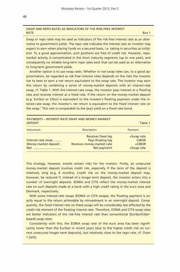
PAYMENTS – INTEREST-RATE SWAP AND MONEY-MARKET DEPOSIT Table 1

Instrument Description Payment

Interest-rate swap ......... Receives fixed leg +Swap rate Pays floating leg -CIBOR

Money-market deposit . Receives money-market rate +CIBOR Net ................................ Net payment +Swap rate

This strategy, however, entails certain risks for the investor. Firstly, an unsecured

money-market deposit involves credit risk, especially if the term of the deposit is

relatively long (e.g. 6 months). Credit risk on the money-market deposit may,

however, be reduced if, instead of a longer-term deposit, the investor enters into a

number of overnight deposits. EONIA and CITA reflect the money-market interest

rate on such deposits made at a bank with a high credit rating in the euro area and

Denmark, respectively.

With some interest-rate swaps (EONIA or CITA swaps), the floating payment is ex-

actly equal to the return achievable by reinvestment in an overnight deposit. Conse-

quently, the fixed interest rate on these swaps will be considerably less affected by the

credit-risk element of the floating interest rate. Therefore, EONIA and CITA swap rates

are better indicators of the risk-free interest rate than conventional (Euribor/Cibor-

based) swap rates.

Consistently with this, the EONIA swap rate of the euro area has been signifi-

cantly lower than the Euribor in recent years (due to the higher credit risk on cur-

rent unsecured longer-term deposits), but relatively close to the repo rate, cf. Chart

1 (left).


49

CONTINUED Box 1

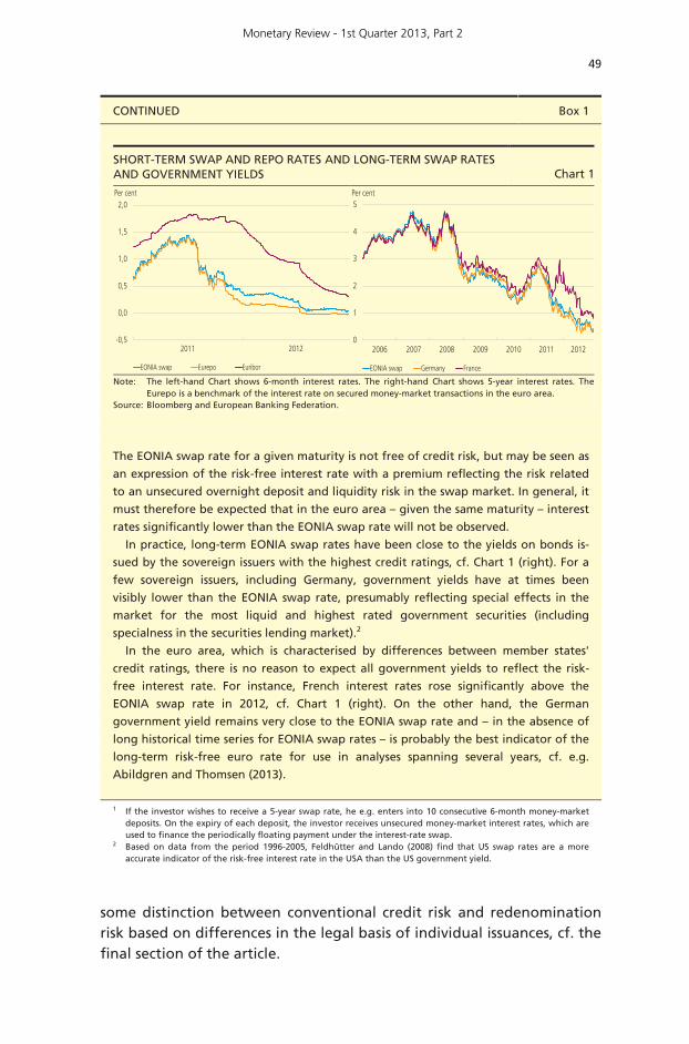
SHORT-TERM SWAP AND REPO RATES AND LONG-TERM SWAP RATES AND GOVERNMENT YIELDS Chart 1

Note: Source:

The left-hand Chart shows 6-month interest rates. The right-hand Chart shows 5-year interest rates. The Eurepo is a benchmark of the interest rate on secured money-market transactions in the euro area. Bloomberg and European Banking Federation.

The EONIA swap rate for a given maturity is not free of credit risk, but may be seen as

an expression of the risk-free interest rate with a premium reflecting the risk related

to an unsecured overnight deposit and liquidity risk in the swap market. In general, it

must therefore be expected that in the euro area – given the same maturity – interest

rates significantly lower than the EONIA swap rate will not be observed.

In practice, long-term EONIA swap rates have been close to the yields on bonds is-

sued by the sovereign issuers with the highest credit ratings, cf. Chart 1 (right). For a

few sovereign issuers, including Germany, government yields have at times been

visibly lower than the EONIA swap rate, presumably reflecting special effects in the

market for the most liquid and highest rated government securities (including

specialness in the securities lending market).2

In the euro area, which is characterised by differences between member states'

credit ratings, there is no reason to expect all government yields to reflect the risk-

free interest rate. For instance, French interest rates rose significantly above the

EONIA swap rate in 2012, cf. Chart 1 (right). On the other hand, the German

government yield remains very close to the EONIA swap rate and – in the absence of

long historical time series for EONIA swap rates – is probably the best indicator of the

long-term risk-free euro rate for use in analyses spanning several years, cf. e.g.

Abildgren and Thomsen (2013).

1 If the investor wishes to receive a 5-year swap rate, he e.g. enters into 10 consecutive 6-month money-market deposits. On the expiry of each deposit, the investor receives unsecured money-market interest rates, which are used to finance the periodically floating payment under the interest-rate swap.

2 Based on data from the period 1996-2005, Feldhütter and Lando (2008) find that US swap rates are a more accurate indicator of the risk-free interest rate in the USA than the US government yield.

some distinction between conventional credit risk and redenomination risk based on differences in the legal basis of individual issuances, cf. the final section of the article.

-0,5

0,0

0,5

1,0

1,5

2,0

EONIA swap Eurepo Euribor

Per cent

2011 20120

1

2

3

4

5

EONIA swap Germany France

Per cent

2006 2007 2008 2009 2010 2011 2012


50

Liquidity spread If, due to external factors, the investor may be compelled to liquidate the bond portfolio before maturity – in addition to credit risk – the investor will be exposed to liquidity risk.1

From the investor's point of view, the immediate liquidity of a bond may be narrowly defined as the loss of value incurred from an imme-diate sale. If the cost of selling a given bond is high – e.g. in the form of a wide spread between bid and ask prices (bid-ask spread) with low order depth or long execution time – this will reduce the value of the bond and contribute to a positive spread to the risk-free interest rate.2

Like in the case of the credit spread, the total compensation for illiquidity, the liquidity spread, may be decomposed into compensation for the expected loss (which depends on the probability of a sale and the expected related costs) and compensation for liquidity risk. The need for premature sale tends to coincide with periods of general market stress when the investor also suffers loss of income from other sources. In other words, the size of the average bid-ask spread is not the only factor to affect the liquidity spread – the expected size of the spread at the exact times of acute sell-off also matters. Hence, the liquidity spread also reflects a liquidity-risk premium.3 Since the liquidity spread is deter-mined by the degree of uncertainty about future liquidity, empirical analyses in which the size of the yield spread is related only to contem-poraneous measures of liquidity (such as the bid-ask spread) may pro-duce misleading results, cf. below. Interaction between credit and liquidity risk Increased uncertainty about the credit rating of an issuer may, in itself, lead to higher investor liquidity risk. The reason is that a widening and more volatile credit spread increases the risk of having to sell the bond. For long-term investors, this may be rooted in a wish to reduce their exposure (measured e.g. by Value-at-Risk) or in internal requirements as to the credit rating of investments. As far as leveraged positions are concerned, (mark-to-market) losses and/or rising margin requirements may necessitate a sale, cf. the discussion in Altenhofen and Lohff (2013).

1 For instance, asset managers may need to divest assets because the underlying investors wish to

redeem funds or because credit facilities are being restricted. 2 Furthermore, the investor requires compensation for trading costs when buying a bond. However,

there is no liquidity risk when buying a bond, since the trading cost is already known. If the bid-ask spread is narrow, compensation for trading costs when buying a bond is limited. 3

Acharya and Pedersen (2005) expand the CAPM model to include liquidity risk and demonstrate that the liquidity-risk premium can be decomposed. The three liquidity-risk components are related to covariation between the individual asset's liquidity and the market portfolio's liquidity, covariation between the individual asset's return and the market portfolio liquidity and covariation between the individual asset's liquidity and the market return, respectively. Based on equity return data during the period 1962-99, the authors find the latter effect to be dominant, i.e. most of the risk premium reflects whether the individual asset is illiquid when the market return is low.


51

In practice, positive covariation between credit and liquidity spreads is to be expected. In "good times", the credit spread is narrow due to low probability of default. At the same time, the liquidity spread is narrow owing to high market liquidity and low probability of a forced sale. Conversely, credit and liquidity spreads both tend to widen in "bad times". Decomposition For purposes of empirical decomposition of the yield spread between two countries, it is useful to decompose interest rates. As discussed above, the yield on a bond issued by country i can be expressed as the sum of the risk-free interest rate (rf), a credit spread (k) and a liquidity spread (l):

t,it,itt,i lkrfr ++=

Therefore, the spread between the interest rate for country i and the risk-free interest rate is:

t,it,itt,i lkrfr +=−

The yield spread between country i and country j for bonds issued in the same currency can be expressed as:

( ) ( )t,jt,it,jt,it,jt,i llkkrr −+−=−

Consequently, the yield spread between, say, two euro area member states is independent of the risk-free interest rate and determined by the relative credit and liquidity spreads. This also entails that a number of implied assumptions are made when the yield spread e.g. between France and Germany is used as the indicator of the credit risk on French government bonds. Firstly, that German government bonds have no credit risk. Secondly, that no (significant) differences exist in the liquidity spreads between the two securities. EMPIRICAL DECOMPOSITION OF YIELD SPREADS BETWEEN EU MEMBER STATES

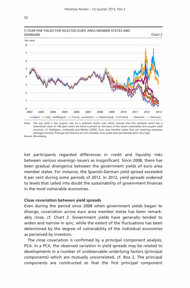
From the introduction of the euro until 2008, yield spreads between euro area member states were narrow, cf. Chart 2,1 indicating that mar-

1 5-year government yields are used throughout the chapter. The reason is that government-yield

spreads are subsequently analysed relative to CDS spreads for which the 5-year maturity segment provides the most consistent basis of comparison.


52

ket participants regarded differences in credit and liquidity risks between various sovereign issuers as insignificant. Since 2008, there has been gradual divergence between the government yields of euro area member states. For instance, the Spanish-German yield spread exceeded 6 per cent during some periods of 2012. In 2012, yield spreads widened to levels that called into doubt the sustainability of government finances in the most vulnerable economies. Close covariation between yield spreads Even during the period since 2008 when government yields began to diverge, covariation across euro area member states has been remark-ably close, cf. Chart 2. Government yields have generally tended to widen and narrow in sync, while the extent of the fluctuations has been determined by the degree of vulnerability of the individual economies as perceived by investors.

The close covariation is confirmed by a principal component analysis, PCA. In a PCA, the observed variation in yield spreads may be related to developments in a number of unobservable underlying factors (principal components) which are mutually uncorrelated, cf. Box 2. The principal components are constructed so that the first principal component

5-YEAR PAR YIELDS FOR SELECTED EURO AREA MEMBER STATES AND DENMARK Chart 2

Note: Source:

The par yield is the coupon rate on a synthetic bullet loan which ensures that the synthetic bond has a theoretical value of 100 (par) when the bond is priced on the basis of the issuer's estimated zero-coupon yield structure, cf. Abildgren, Lindewald and Nielsen (2005). Euro area member states that are receiving assistance packages (Ireland, Portugal and Greece) are not included, since yields have periodically been very high. Bloomberg.

0

1

2

3

4

5

6

7

8

2002 2003 2004 2005 2006 2007 2008 2009 2010 2011 2012 2013

Spain Italy Belgium France Austria Netherlands Finland Denmark Germany

Per cent


53

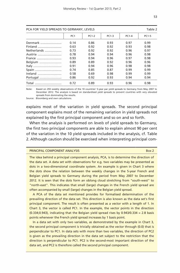
explains most of the variation in yield spreads. The second principal component explains most of the remaining variation in yield spreads not explained by the first principal component and so on and so forth.

When the analysis is performed on levels of yield spreads to Germany, the first two principal components are able to explain almost 90 per cent of the variation in the 10 yield spreads included in the analysis, cf. Table 2. Although caution should be exercised when interpreting principal com-

PCA FOR YIELD SPREADS TO GERMANY, LEVELS Table 2

PC1 PC1-2 PC1-3 PC1-4 PC1-5

Denmark ........................ 0.14 0.86 0.93 0.97 0.99 Finland ........................... 0.63 0.92 0.92 0.93 0.98 Netherlands ................... 0.73 0.92 0.92 0.96 0.97 Austria ........................... 0.78 0.94 0.94 0.96 0.98 France ............................ 0.93 0.94 0.96 0.97 0.98 Belgium ......................... 0.89 0.89 0.92 0.96 0.96 Italy ................................ 0.91 0.94 0.96 0.98 0.98 Spain .............................. 0.74 0.85 0.87 0.99 0.99 Ireland ........................... 0.58 0.69 0.98 0.99 0.99 Portugal ......................... 0.86 0.92 0.93 0.94 0.94

Total .............................. 0.72 0.89 0.93 0.96 0.98

Note: Based on 293 weekly observations of the 10 countries' 5-year par yield spreads to Germany from May 2007 to December 2012. The analysis is based on standardised yield spreads to prevent countries with very elevated spreads from dominating the results.

Source: Bloomberg and own calculations.

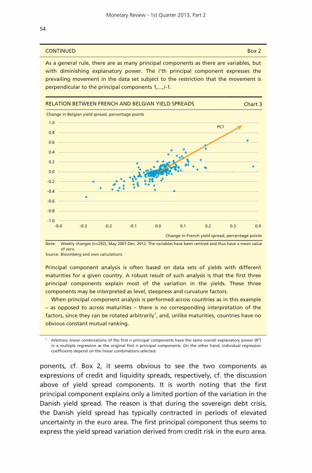
PRINCIPAL COMPONENT ANALYSIS Box 2

The idea behind a principal component analysis, PCA, is to determine the direction of

the data set. A data set with observations for e.g. two variables may be presented as

dots in a two-dimensional coordinate system. An example is given in Chart 3 where

the dots show the relation between the weekly changes in the 5-year French and

Belgian yield spreads to Germany during the period from May 2007 to December

2012. It is seen that the dots form an oblong cloud stretching from "south-west" to

"north-east". This indicates that small (large) changes in the French yield spread are

often accompanied by small (large) changes in the Belgian yield spread.

A PCA of the data set mentioned provides for formalised determination of the

prevailing direction of the data set. This direction is also known as the data set's first

principal component. The result is often presented as a vector with a length of 1. In

Chart 3, the vector is called PC1. In the example, the vector points in the direction

(0.334;0.943), indicating that the Belgian yield spread rises by 0.943/0.334 = 2.8 basis

points whenever the French yield spread increases by 1 basis point.

In a data set with only two variables, as demonstrated by the example in Chart 3,

the second principal component is trivially obtained as the vector through (0.0) that is

perpendicular to PC1. In data sets with more than two variables, the direction of PC2

is given as the prevailing direction in the data set subject to the restriction that the

direction is perpendicular to PC1. PC2 is the second-most important direction of the

data set, and PC2 is therefore called the second principal component.


54

CONTINUED Box 2

As a general rule, there are as many principal components as there are variables, but

with diminishing explanatory power. The i'th principal component expresses the

prevailing movement in the data set subject to the restriction that the movement is

perpendicular to the principal components 1,...,i-1.

RELATION BETWEEN FRENCH AND BELGIAN YIELD SPREADS Chart 3

Note: Source:

Weekly changes (n=292), May 2007-Dec. 2012. The variables have been centred and thus have a mean value of zero. Bloomberg and own calculations.

Principal component analysis is often based on data sets of yields with different

maturities for a given country. A robust result of such analysis is that the first three

principal components explain most of the variation in the yields. These three

components may be interpreted as level, steepness and curvature factors.

When principal component analysis is performed across countries as in this example

– as opposed to across maturities – there is no corresponding interpretation of the

factors, since they can be rotated arbitrarily1, and, unlike maturities, countries have no

obvious constant mutual ranking.

1 Arbitrary linear combinations of the first n principal components have the same overall explanatory power (R2) in a multiple regression as the original first n principal components. On the other hand, individual regression coefficients depend on the linear combinations selected.

ponents, cf. Box 2, it seems obvious to see the two components as expressions of credit and liquidity spreads, respectively, cf. the discussion above of yield spread components. It is worth noting that the first principal component explains only a limited portion of the variation in the Danish yield spread. The reason is that during the sovereign debt crisis, the Danish yield spread has typically contracted in periods of elevated uncertainty in the euro area. The first principal component thus seems to express the yield spread variation derived from credit risk in the euro area.

-1.0

-0.8

-0.6

-0.4

-0.2

0.0

0.2

0.4

0.6

0.8

1.0

-0.4 -0.3 -0.2 -0.1 0.0 0.1 0.2 0.3 0.4

Change in French yield spread, percentage points

Change in Belgian yield spread, percentage points

PC1


55

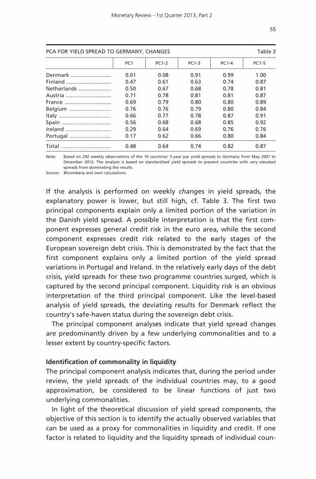
If the analysis is performed on weekly changes in yield spreads, the explanatory power is lower, but still high, cf. Table 3. The first two principal components explain only a limited portion of the variation in the Danish yield spread. A possible interpretation is that the first com-ponent expresses general credit risk in the euro area, while the second component expresses credit risk related to the early stages of the European sovereign debt crisis. This is demonstrated by the fact that the first component explains only a limited portion of the yield spread variations in Portugal and Ireland. In the relatively early days of the debt crisis, yield spreads for these two programme countries surged, which is captured by the second principal component. Liquidity risk is an obvious interpretation of the third principal component. Like the level-based analysis of yield spreads, the deviating results for Denmark reflect the country's safe-haven status during the sovereign debt crisis.

The principal component analyses indicate that yield spread changes are predominantly driven by a few underlying commonalities and to a lesser extent by country-specific factors.

Identification of commonality in liquidity The principal component analysis indicates that, during the period under review, the yield spreads of the individual countries may, to a good approximation, be considered to be linear functions of just two underlying commonalities.

In light of the theoretical discussion of yield spread components, the objective of this section is to identify the actually observed variables that can be used as a proxy for commonalities in liquidity and credit. If one factor is related to liquidity and the liquidity spreads of individual coun-

PCA FOR YIELD SPREAD TO GERMANY, CHANGES Table 3

PC1 PC1-2 PC1-3 PC1-4 PC1-5

Denmark .......................... 0.01 0.08 0.91 0.99 1.00 Finland ............................. 0.47 0.61 0.63 0.74 0.87 Netherlands ..................... 0.50 0.67 0.68 0.78 0.81 Austria ............................. 0.71 0.78 0.81 0.81 0.87 France .............................. 0.69 0.79 0.80 0.80 0.89 Belgium ........................... 0.76 0.76 0.79 0.80 0.84 Italy .................................. 0.66 0.77 0.78 0.87 0.91 Spain ................................ 0.56 0.68 0.68 0.85 0.92 Ireland ............................. 0.29 0.64 0.69 0.76 0.76 Portugal ........................... 0.17 0.62 0.66 0.80 0.84

Total ................................ 0.48 0.64 0.74 0.82 0.87

Note: Based on 292 weekly observations of the 10 countries' 5-year par yield spreads to Germany from May 2007 to December 2012. The analysis is based on standardised yield spreads to prevent countries with very elevated spreads from dominating the results.



56

tries are linear functions of this commonality in liquidity, the difference in liquidity spreads will also be a linear function of this commonality.

This entails that if a liquidity spread can be identified with relative precision for a few countries, this spread may be used to explain more general changes in yield spreads.

A possible strategy for identifying the unobserved liquidity factor (up to a constant) is to observe two bonds with the same credit risk, but different liquidity. Changes in the yield spread between the bonds will be driven by the liquidity factor. Using the notation from the previous section: if t,jt,i kk = , it applies that

t,jt,itt,jt,i llrr −=−

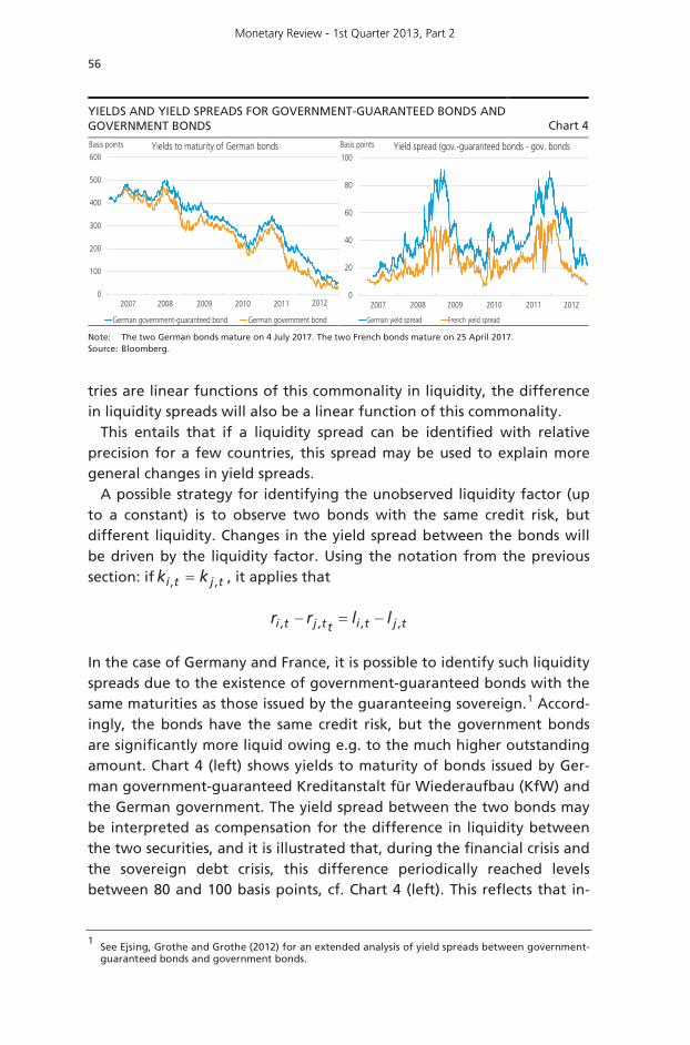
In the case of Germany and France, it is possible to identify such liquidity spreads due to the existence of government-guaranteed bonds with the same maturities as those issued by the guaranteeing sovereign.1 Accord-ingly, the bonds have the same credit risk, but the government bonds are significantly more liquid owing e.g. to the much higher outstanding amount. Chart 4 (left) shows yields to maturity of bonds issued by Ger-man government-guaranteed Kreditanstalt für Wiederaufbau (KfW) and the German government. The yield spread between the two bonds may be interpreted as compensation for the difference in liquidity between the two securities, and it is illustrated that, during the financial crisis and the sovereign debt crisis, this difference periodically reached levels between 80 and 100 basis points, cf. Chart 4 (left). This reflects that in-

1 See Ejsing, Grothe and Grothe (2012) for an extended analysis of yield spreads between government-

guaranteed bonds and government bonds.

YIELDS AND YIELD SPREADS FOR GOVERNMENT-GUARANTEED BONDS AND GOVERNMENT BONDS Chart 4

Note: Source:

The two German bonds mature on 4 July 2017. The two French bonds mature on 25 April 2017. Bloomberg.

0

100

200

300

400

500

600

German government-guaranteed bond German government bond

Basis points Yields to maturity of German bonds

2007 2008 2009 2010 2011 20120

20

40

60

80

100

German yield spread French yield spread

Basis points Yield spread (gov.-guaranteed bonds - gov. bonds

2007 2008 2009 2010 2011 2012


57

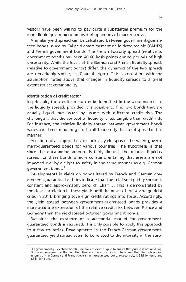
vestors have been willing to pay quite a substantial premium for the more liquid government bonds during periods of market stress.

A similar yield spread can be calculated between government-guaran-teed bonds issued by Caisse d'amortissement de la dette sociale (CADES) and French government bonds. The French liquidity spread (relative to government bonds) has been 40-60 basis points during periods of high uncertainty. While the levels of the German and French liquidity spreads (relative to government bonds) differ, the dynamics of the two spreads are remarkably similar, cf. Chart 4 (right). This is consistent with the assumption noted above that changes in liquidity spreads to a great extent reflect commonality. Identification of credit factor In principle, the credit spread can be identified in the same manner as the liquidity spread, provided it is possible to find two bonds that are equally liquid, but issued by issuers with different credit risk. The challenge is that the concept of liquidity is less tangible than credit risk. For instance, the relative liquidity spread between government bonds varies over time, rendering it difficult to identify the credit spread in this manner.

An alternative approach is to look at yield spreads between govern-ment-guaranteed bonds for various countries. The hypothesis is that since the outstanding amount is fairly limited, the relative liquidity spread for these bonds is more constant, entailing that assets are not impacted e.g. by a flight to safety in the same manner as e.g. German government bonds.1

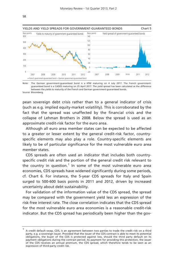
Developments in yields on bonds issued by French and German gov-ernment-guaranteed entities indicate that the relative liquidity spread is constant and approximately zero, cf. Chart 5. This is demonstrated by the close correlation in these yields until the onset of the sovereign debt crisis in 2011, bringing sovereign credit ratings into focus. Accordingly, the yield spread between government-guaranteed bonds provides a more accurate expression of the relative credit risk between France and Germany than the yield spread between government bonds.

But since the existence of a substantial market for government-guaranteed bonds is required, it is only possible to apply this approach to a few countries. Developments in the French-German government-guaranteed yield spread seem to be related to the intensity of the Euro-

1 The government-guaranteed bonds used are sufficiently liquid to ensure that pricing is not arbitrary.

This is underpinned by the fact that they are traded on a daily basis and that the outstanding amount of the German and French government-guaranteed bond, respectively, is 5 billion euro and 3.8 billion euro.


58

pean sovereign debt crisis rather than to a general indicator of crisis (such as e.g. implied equity-market volatility). This is corroborated by the fact that the spread was unaffected by the financial crisis and the collapse of Lehman Brothers in 2008. Below the spread is used as an approximate credit-risk factor for the euro area.

Although all euro area member states can be expected to be affected to a greater or lesser extent by the general credit-risk factor, country-specific elements may also play a role. Country-specific elements are likely to be of particular significance for the most vulnerable euro area member states.

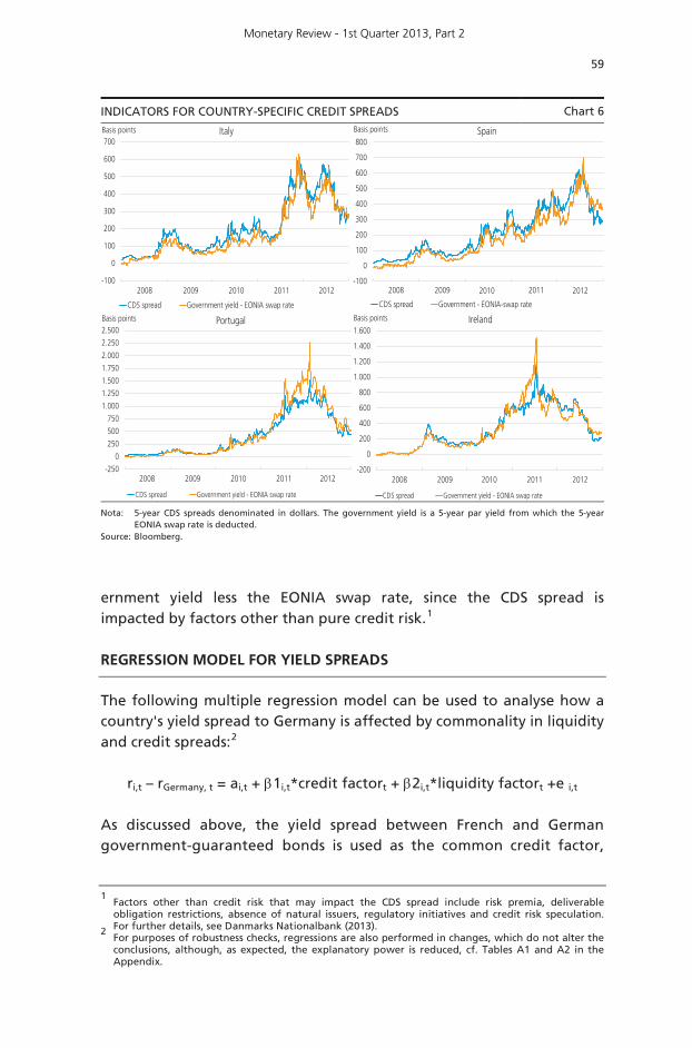
CDS spreads are often used an indicator that includes both country-specific credit risk and the portion of the general credit risk relevant to the country in question.1 In some of the most vulnerable euro area economies, CDS spreads have widened significantly during some periods, cf. Chart 6. For instance, the 5-year CDS spreads for Italy and Spain surged to 500-600 basis points in 2011 and 2012, driven by increased uncertainty about debt sustainability.

For validation of the information value of the CDS spread, the spread may be compared with the government yield less an expression of the risk-free interest rate. The close correlation indicates that the CDS spread for the most vulnerable euro area economies is a reasonable credit-risk indicator. But the CDS spread has periodically been higher than the gov-

1 A credit default swap, CDS, is an agreement between two parties to trade the credit risk on a third

party, e.g. a sovereign issuer. Provided that the issuer of the CDS contract is able to meet its potential obligations, the buyer of the CDS is protected against loss, should the third party default on its payment obligations during the contract period. As payment for providing this protection, the issuer of the CDS receives an annual premium, the CDS spread, which therefore tends to be seen as an expression of third-party credit risk.

YIELDS AND YIELD SPREADS FOR GOVERNMENT-GUARANTEED BONDS Chart 5

Note: Source:

The German government-guaranteed bond is a KfW maturing on 4 July 2017. The French government-guaranteed bond is a CADES maturing on 25 April 2017. The yield spread has been calculated as the difference between the yields to maturity of the French and German government-guaranteed bonds. Bloomberg.

0

100

200

300

400

500

600

French government-guaranteed bond German government-guaranteed bond

Basis points Yields to maturity of government-guaranteed bonds

2007 2008 2009 2010 2011 2012-20

0

20

40

60

80

100

120

140Basis points YIeld spread of government-guaranteed bonds

2007 2008 2009 2010 2011 2012


59

INDICATORS FOR COUNTRY-SPECIFIC CREDIT SPREADS Chart 6

Nota: Source:

5-year CDS spreads denominated in dollars. The government yield is a 5-year par yield from which the 5-year EONIA swap rate is deducted. Bloomberg.

ernment yield less the EONIA swap rate, since the CDS spread is impacted by factors other than pure credit risk.1

REGRESSION MODEL FOR YIELD SPREADS

The following multiple regression model can be used to analyse how a country's yield spread to Germany is affected by commonality in liquidity and credit spreads:2

ri,t – rGermany, t = ai,t + β1i,t*credit factort + β2i,t*liquidity factort +e i,t As discussed above, the yield spread between French and German government-guaranteed bonds is used as the common credit factor,

1 Factors other than credit risk that may impact the CDS spread include risk premia, deliverable

obligation restrictions, absence of natural issuers, regulatory initiatives and credit risk speculation. For further details, see Danmarks Nationalbank (2013). 2

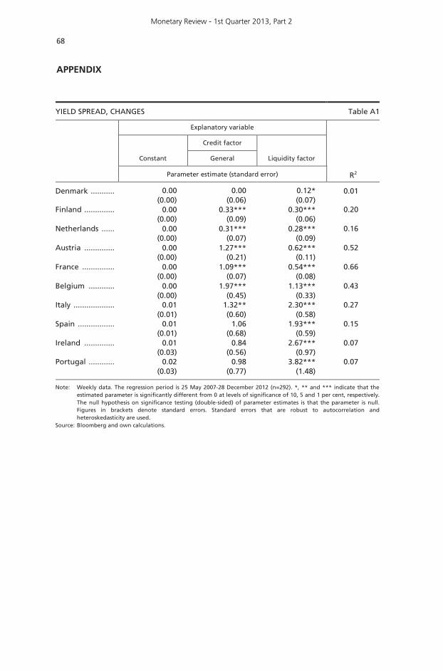
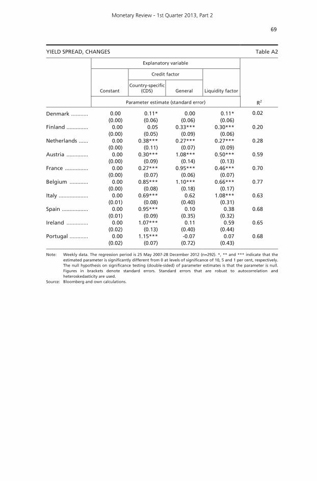
For purposes of robustness checks, regressions are also performed in changes, which do not alter the conclusions, although, as expected, the explanatory power is reduced, cf. Tables A1 and A2 in the Appendix.

-100

0

100

200

300

400

500

600

700

CDS spread Government yield - EONIA swap rate

Basis points Italy

2008 2009 2010 2011 2012-100

0

100

200

300

400

500

600

700

800

CDS spread Government - EONIA-swap rate

Basis points Spain

2008 2009 2010 2011 2012

-250

0

250

500

750

1.000

1.250

1.500

1.750

2.000

2.250

2.500


Basis points Portugal

2008 2009 2010 2011 2012-200

0

200

400

600

800

1.000

1.200

1.400

1.600


Basis points Ireland

2008 2009 2010 2011 2012


60

the yield spread between German government-guaranteed bonds

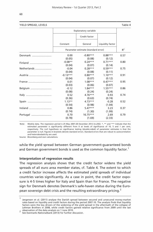
and German government bonds is used as the common liquidity factor.1 Interpretation of regression results The regression analysis shows that the credit factor widens the yield spreads of all euro area member states, cf. Table 4. The extent to which a credit factor increase affects the estimated yield spreads of individual countries varies significantly. As a case in point, the credit factor expo-sure is 4-5 times higher for Italy and Spain than for France. The negative sign for Denmark denotes Denmark's safe-haven status during the Euro-pean sovereign debt crisis and the resulting extraordinary pricing.2

1 Jørgensen et al. (2011) analyse the Danish spread between secured and unsecured money-market

rates based on liquidity and credit factors during the period 2007-10. The analysis finds that liquidity factors were the key drivers of the widening of the yield spread in the aftermath of the collapse of Lehman Brothers in 2008, while credit factors gained relative significance from 2009 until the last observation of the data analysis on 1 June 2010. 2

See Danmarks Nationalbank (2013) for further discussion.

YIELD SPREAD, LEVELS Table 4

Explanatory variable

Constant

Credit factor

Liquidity factor

General

Parameter estimate (standard error) R2

Denmark .......................... 0.00 (0.05)

-0.80*** (0.08)

0.88*** (0.12)

0.57

Finland ............................. -0.08** (0.04)

0.24*** (0.07)

0.71*** (0.14)

0.80

Netherlands ...................... -0.04 (0.04)

0.28*** (0.08)

0.59*** (0.11)

0.75

Austria .............................. -0.13*** (0.04)

0.80*** (0.07)

1.10*** (0.12)

0.91

France ............................... 0.01 (0.03)

1.08*** (0.06)

0.47*** (0.07)

0.95

Belgium ............................ -0.12 (0.08)

1.84*** (0.24)

1.55*** (0.24)

0.86

Italy .................................. 0.52 (0.36)

4.76*** (0.63)

0.93 (0.74)

0.74

Spain ................................ 1.13** (0.54)

4.73*** (0.98)

-0.28 (1.04)

0.52

Ireland .............................. 0.86 (0.74)

5.47*** (1.30)

3.23 (1.99)

0.37

Portugal ........................... 0.70 (0.78)

16.75*** (1.69)

2.69 (2.33)

0.79

Note: Weekly data. The regression period is 25 May 2007-28 December 2012 (n=292). *, ** and *** indicate that the estimated parameter is significantly different from 0 at levels of significance of 10, 5 and 1 per cent, respectively. The null hypothesis on significance testing (double-sided) of parameter estimates is that the parameter is null. Figures in brackets denote standard errors. Standard errors that are robust to autocorrelation and heteroskedasticity are used.


while


61

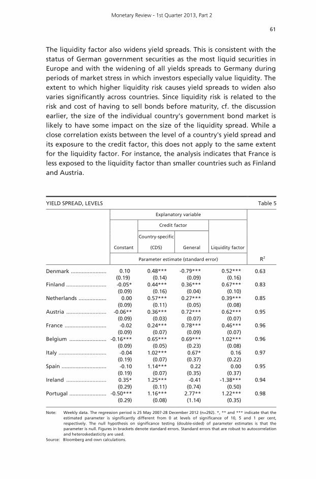
The liquidity factor also widens yield spreads. This is consistent with the status of German government securities as the most liquid securities in Europe and with the widening of all yields spreads to Germany during periods of market stress in which investors especially value liquidity. The extent to which higher liquidity risk causes yield spreads to widen also varies significantly across countries. Since liquidity risk is related to the risk and cost of having to sell bonds before maturity, cf. the discussion earlier, the size of the individual country's government bond market is likely to have some impact on the size of the liquidity spread. While a close correlation exists between the level of a country's yield spread and its exposure to the credit factor, this does not apply to the same extent for the liquidity factor. For instance, the analysis indicates that France is less exposed to the liquidity factor than smaller countries such as Finland and Austria.

YIELD SPREAD, LEVELS Table 5


Constant

Credit factor

Liquidity factor

Country-specific

(CDS)

General


Denmark ....................... 0.10

(0.19) 0.48***

(0.14) -0.79***

(0.09) 0.52***

(0.16)

0.63

Finland .......................... -0.05* (0.09)

0.44*** (0.16)

0.36*** (0.04)

0.67*** (0.10)

0.83

Netherlands .................. 0.00 (0.09)

0.57*** (0.11)

0.27*** (0.05)

0.39*** (0.08)

0.85

Austria .......................... -0.06** (0.09)

0.36*** (0.03)

0.72*** (0.07)

0.62*** (0.07)

0.95

France ........................... -0.02 (0.09)

0.24*** (0.07)

0.78*** (0.09)

0.46*** (0.07)

0.96

Belgium ........................ -0.16*** (0.09)

0.65*** (0.05)

0.69*** (0.23)

1.02*** (0.08)

0.96

Italy ............................... -0.04 (0.19)

1.02*** (0.07)

0.67* (0.37)

0.16 (0.22)

0.97

Spain ............................. -0.10 (0.19)

1.14*** (0.07)

0.22 (0.35)

0.00 (0.37)

0.95

Ireland .......................... 0.35* (0.29)

1.25*** (0.11)

-0.41 (0.74)

-1.38*** (0.50)

0.94

Portugal ........................ -0.50*** (0.29)

1.16*** (0.08)

2.77** (1.14)

1.22*** (0.35)

0.98




62

The explanatory power (R2) of the model is generally high for the individual countries. But developments in the Irish and Spanish yield spreads, in particular, are not explained all that well by the two commonalities, indicating that country-specific credit risk has periodically had a great impact, especially on vulnerable economies. Inclusion of the individual countries' CDS spreads in the regression equation above allows for a better explanation of developments in the Irish and Southern European yield spreads, cf. Table 5.

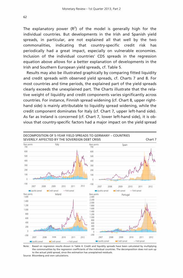
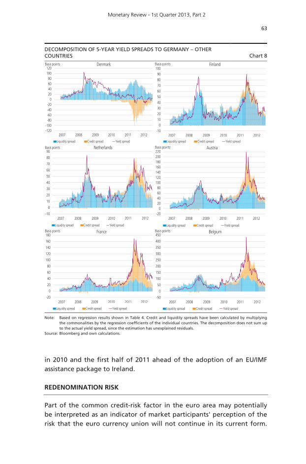
Results may also be illustrated graphically by comparing fitted liquidity and credit spreads with observed yield spreads, cf. Charts 7 and 8. For most countries and time periods, the explained part of the yield spreads clearly exceeds the unexplained part. The Charts illustrate that the rela-tive weight of liquidity and credit components varies significantly across countries. For instance, Finnish spread widening (cf. Chart 8, upper right-hand side) is mainly attributable to liquidity spread widening, while the credit component dominates for Italy (cf. Chart 7, upper left-hand side). As far as Ireland is concerned (cf. Chart 7, lower left-hand side), it is ob-vious that country-specific factors had a major impact on the yield spread

DECOMPOSITION OF 5-YEAR YIELD SPREADS TO GERMANY – COUNTRIES SEVERELY AFFECTED BY THE SOVEREIGN DEBT CRISIS Chart 7

Note: Source:

Based on regression results shown in Table 4. Credit and liquidity spreads have been calculated by multiplying the commonalities by the regression coefficients of the individual countries. The decomposition does not sum up to the actual yield spread, since the estimation has unexplained residuals. Bloomberg and own calculations.

-100

0

100

200

300

400

500

600

700

Liquidity spread Credit spread Yield spread

Basis points Italy

2007 2008 2009 2010 2011 2012-100

0

100

200

300

400

500

600

700


Basis points Spain

2007 2008 2009 2010 2011 2012

-200

0

200

400

600

800

1.000

1.200

1.400

1.600


Basis points Ireland

2007 2008 2009 2010 2011 2012-200

0200400600800

1.0001.2001.4001.6001.8002.0002.2002.400


Basis points Portugal

2007 2008 2009 2010 2011 2012


63

in 2010 and the first half of 2011 ahead of the adoption of an EU/IMF assistance package to Ireland. REDENOMINATION RISK

Part of the common credit-risk factor in the euro area may potentially be interpreted as an indicator of market participants' perception of the risk that the euro currency union will not continue in its current form.

DECOMPOSITION OF 5-YEAR YIELD SPREADS TO GERMANY – OTHER COUNTRIES Chart 8

Note: Source:

Based on regression results shown in Table 4. Credit and liquidity spreads have been calculated by multiplying the commonalities by the regression coefficients of the individual countries. The decomposition does not sum up to the actual yield spread, since the estimation has unexplained residuals. Bloomberg and own calculations.

-120-100-80-60-40-20

020406080

100120


Basis points Denmark

2007 2008 2009 2010 2011 2012-10

0

10

20

30

40

50

60

70

80

90

100


Basis points Finland

2007 2008 2009 2010 2011 2012

-10

0

10

20

30

40

50

60

70

80

90


Basis points Netherlands

2007 2008 2009 2010 20122011-20

020406080

100120140160180200220


Basis points Austria

2007 2008 2009 2010 2011 2012

-20

0

20

40

60

80

100

120

140

160

180


Basis points France

2007 2008 2009 2010 2011 2012-50

0

50

100

150

200

250

300

350

400

450


Basis points Belgium

2007 2008 2009 2010 2011 2012


64

Certain market participants have attached some probability to this sce-nario, and as the rationale for its latest purchasing programme, Outright Monetary Transactions, OMT, the ECB cited the need to secure the continued existence of the currency union.1

If a country exits from the euro area and lets its currency depreciate, the effect for an investor who originally purchased the country's bonds as euro claims will be equivalent to a debt write-down in case of en-forced conversion of the bonds into the new currency. This makes it dif-ficult to draw an empirical distinction between conventional credit risk and redenomination risk.

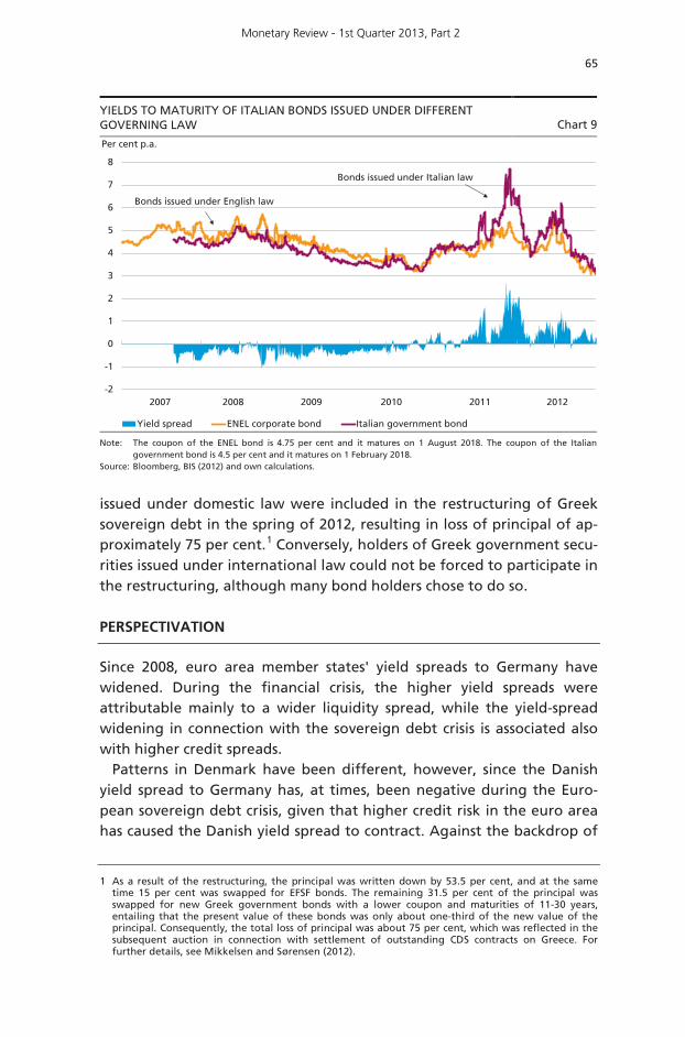
By comparing bonds issued under domestic and international law, re-spectively, the Bank for International Settlements, BIS, (2012) has sought to find highly approximate indicators of the redenomination risk. The idea behind the indicator is that, in principle, a sovereign issuer may redenominate the currency of a bond subject to domestic law, while this may be considerably more difficult for bonds subject to international law (e.g. English law).2 As a case in point, BIS (2012) looks at Italian gov-ernment bonds issued under domestic law and corporate bonds issued under international law by the partly government-owned Italian energy company, ENEL.3 At the height of the European sovereign debt crisis, the Italian government yield was significantly higher than the yield on ENEL's corporate bonds, which could be an indication of increased re-denomination risk, cf. Chart 9. The widened yield spread contrasts with a scenario with limited market uncertainty where the spread is typically negative due to lower liquidity of ENEL's bonds.4 At the same time, it is worth noting that the yield spread increased only slightly in the after-math of the collapse of Lehman Brothers, indicating that the yield spread is a euro crisis factor more than a general financial crisis factor.5

Bonds issued under international law may in certain cases serve as pro-tection against debt restructuring. For instance, Greek government bonds

1 "Risk premia that are related to fears of the reversibility of the euro are unacceptable, and they need

to be addressed in a fundamental manner. The euro is irreversible", ECB Monthly Bulletin, August 2012, p. 5. 2

Other factors besides the governing law for the bonds may have an impact on the possibility of redenominating debt. For instance, it cannot be ruled out that bonds subject to international law may be redenominated if the primary attachment is assessed to be to the domestic market rather than an international market (e.g. if the bonds are listed only on the domestic stock exchange). Moreover, Nordvig et al. (2011) also mention that if a euro exit happens in a multilaterally agreed fashion, it cannot be ruled out that bonds subject to international law may be redenominated. 3

The Italian government is the majority shareholder of the country's largest energy company, ENEL, and therefore it can be assumed that there is no significant deviation between the company's credit risk and the credit risk of the Italian government. This is underpinned e.g. by credit rating agencies typically reassessing ENEL's rating with reference to changes in the Italian government's credit rating, indicating an implied government guarantee. 4

The outstanding amount of ENEL's corporate bond maturing on 1 August 2018 is about 0.75 billion euro, while the outstanding amount of the comparable Italian government bond is around 25 billion euro.

5 See Danmarks Nationalbank (2013) for further discussion.


65

issued under domestic law were included in the restructuring of Greek sovereign debt in the spring of 2012, resulting in loss of principal of ap-proximately 75 per cent.1 Conversely, holders of Greek government secu-rities issued under international law could not be forced to participate in the restructuring, although many bond holders chose to do so. PERSPECTIVATION

Since 2008, euro area member states' yield spreads to Germany have widened. During the financial crisis, the higher yield spreads were attributable mainly to a wider liquidity spread, while the yield-spread widening in connection with the sovereign debt crisis is associated also with higher credit spreads.

Patterns in Denmark have been different, however, since the Danish yield spread to Germany has, at times, been negative during the Euro-pean sovereign debt crisis, given that higher credit risk in the euro area has caused the Danish yield spread to contract. Against the backdrop of

1 As a result of the restructuring, the principal was written down by 53.5 per cent, and at the same time 15 per cent was swapped for EFSF bonds. The remaining 31.5 per cent of the principal was swapped for new Greek government bonds with a lower coupon and maturities of 11-30 years, entailing that the present value of these bonds was only about one-third of the new value of the principal. Consequently, the total loss of principal was about 75 per cent, which was reflected in the subsequent auction in connection with settlement of outstanding CDS contracts on Greece. For further details, see Mikkelsen and Sørensen (2012).

YIELDS TO MATURITY OF ITALIAN BONDS ISSUED UNDER DIFFERENT GOVERNING LAW Chart 9

Note: Source:

The coupon of the ENEL bond is 4.75 per cent and it matures on 1 August 2018. The coupon of the Italian government bond is 4.5 per cent and it matures on 1 February 2018. Bloomberg, BIS (2012) and own calculations.

-2

-1

0

1

2

3

4

5

6

7

8

Yield spread ENEL corporate bond Italian government bond

Per cent p.a.

Bonds issued under Italian law

Bonds issued under English law

2007 2008 2009 2010 2011 2012


66

increased uncertainty about euro area developments and the costs of resolving the debt crisis, demand for non-euro denominated government securities with a high credit rating has periodically increased. Danish government securities have the highest credit rating and, therefore, have been attractive to investors, resulting in falling Danish yields and lower government borrowing costs. LITERATURE

Abildgren, Kim, Jacob Lindewald and Michal Chr. Nielsen (2005), The 10-year yield spread between Denmark and Germany, Danmarks Nationalbank, Monetary Review, 1st Quarter. Abildgren, Kim and Casper Ristorp Thomsen (2013), Macroeconomic determinants of the development in yield spreads to Germany, Danmarks Nationalbank, Monetary Review, 1st Quarter, Part 2.

Acharya, Viral V. and Lasse H. Pedersen (2005), Asset pricing with liquidity risk, Journal of Financial Economics, Vol. 77(2). Altenhofen, David and Jane Lee Lohff (2013), Market dynamics, frictions and contagion effects, Danmarks Nationalbank, Monetary Review, 1st Quarter, Part 2. BIS (2012), BIS Quarterly Review: International banking and financial market developments, December. Danmarks Nationalbank (2013), Danish government borrowing and debt 2012. Ejsing, Jacob W., Magdalena Grothe and Oliver Grothe (2012), Liquidity and credit risk premia in government bond yields, ECB Working Paper, No. 1440, June. Feldhütter, Peter and David Lando (2008), Decomposing swap spreads, Journal of Financial Economics, Vol. 88(2). Huang, Chi-fu and Robert H. Litzenberger (1988), Foundations for financial economics, North-Holland. Jørgensen, Anders, Paul Lassenius Kramp, Carina Moselund Jensen and Lars Risbjerg (2011), The money and foreign-exchange markets during the crisis, Danmarks Nationalbank, Monetary Review, 2nd Quarter, Part 2.


67

Longstaff, Francis A., Jun Pan, Lasse H. Pedersen and Kenneth J. Singleton (2011), How sovereign is sovereign credit risk?, American Economic Journal: Macroeconomics, Vol. 3(2).

Mikkelsen, Uffe and Søren Vester Sørensen (2012), Write-down of Greek debt and new EU/IMF loan programme, Danmarks Nationalbank, Monetary Review, 1st Quarter, Part 1. Nordvig, Jens, Nick Firoozye and Charles St-Arnaud (2011), Currency risk in a eurozone break-up – legal aspects, Nomura, November. Reinhart, Carmen M. and Kenneth S. Rogoff (2009), This time is different: Eight centuries of financial folly, Princeton University Press.


68

APPENDIX

YIELD SPREAD, CHANGES Table A1


Constant

Credit factor

Liquidity factor General


Denmark ........... 0.00

(0.00) 0.00

(0.06) 0.12* (0.07)

0.01

Finland .............. 0.00 (0.00)

0.33*** (0.09)

0.30*** (0.06)

0.20

Netherlands ...... 0.00 (0.00)

0.31*** (0.07)

0.28*** (0.09)

0.16

Austria .............. 0.00 (0.00)

1.27*** (0.21)

0.62*** (0.11)

0.52

France ............... 0.00 (0.00)

1.09*** (0.07)

0.54*** (0.08)

0.66

Belgium ............ 0.00 (0.00)

1.97*** (0.45)

1.13*** (0.33)

0.43

Italy ................... 0.01 (0.01)

1.32** (0.60)

2.30*** (0.58)

0.27

Spain ................. 0.01 (0.01)

1.06 (0.68)

1.93*** (0.59)

0.15

Ireland .............. 0.01 (0.03)

0.84 (0.56)

2.67*** (0.97)

0.07

Portugal ............ 0.02 (0.03)

0.98 (0.77)

3.82*** (1.48)

0.07




69

YIELD SPREAD, CHANGES Table A2


Constant

Credit factor

Liquidity factor Country-specific

(CDS)

General


Denmark ........... 0.00

(0.00) 0.11* (0.06)

0.00 (0.06)

0.11* (0.06)

0.02

Finland .............. 0.00 (0.00)

0.05 (0.05)

0.33*** (0.09)

0.30*** (0.06)

0.20

Netherlands ...... 0.00 (0.00)

0.38*** (0.11)

0.27*** (0.07)

0.27*** (0.09)

0.28

Austria .............. 0.00 (0.00)

0.30*** (0.09)

1.08*** (0.14)

0.50*** (0.13)

0.59

France ............... 0.00 (0.00)

0.27*** (0.07)

0.95*** (0.06)

0.46*** (0.07)

0.70

Belgium ............ 0.00 (0.00)

0.85*** (0.08)

1.10*** (0.18)

0.66*** (0.17)

0.77

Italy ................... 0.00 (0.01)

0.69*** (0.08)

0.62 (0.40)

1.08*** (0.31)

0.63

Spain ................. 0.00 (0.01)

0.95*** (0.09)

0.10 (0.35)

0.38 (0.32)

0.68

Ireland .............. 0.00 (0.02)

1.07*** (0.13)

0.11 (0.40)

0.59 (0.44)

0.65

Portugal ............ 0.00 (0.02)

1.15*** (0.07)

-0.07 (0.72)

0.07 (0.43)

0.68


