


Languages
Pages
Legal


Dynamic programmingDynamic programming is typically applied to optimization problems.There can be many possible solutions in optimization problems. Each solution has a value, and we wish to find a solution with the optimal (minimum or maximum) value.

Manufacturing problem
7 9 3 4
3
2
2
4
8 4
8 5 6 4 5 7
2
2
3
1
1
2
3
2
4
1
Chassis enters
Assembly line 1
Completed auto exits
Assembly line 2
StationS1,1
StationS1,2
StationS1,3
StationS1,4
StationS1,5
StationS1,6
StationS2,1
StationS2,2
StationS2,3
StationS2,4
StationS2,5
StationS2,6

Brute-forceCheck every way through a factory and choose the fastest way.
AnalysisChecking = O(n) time per way.2n possible ways to choose stations.Worst-case running time = O(n2n)
= exponential time.
It is infeasible!

Structure of manufacturing problemAn optimal solution to a problem (finding the fastest way though station Si,j) contains within it an optimal solution to subproblems (finding the fastest way through either S1,j−1 or S2,j−1)Suppose that the fastest way through station S1,j is either
the fastest way through station S1,j−1 and then directly through station S1,j, orthe fastest way through station S2,j−1, a transfer from line 1to line 1, and then through station S1,j.
Suppose that the fastest way through station S1,j is through station S1,j−1. The key observation is that the chassis must have taken a fastest way from the starting point through station S1,j−1.

Recursive solutiondenote the fastest possible time to get a chassis from the starting point through station Sij.
Our ultimate goal is:f * = min(f1[n] + x1, f2[n] + x2).
denote an entry time for the chassis to enter assembly line i.denote an exit time for the completed auto to exit assembly line i.denote the assembly time required at station Sij.denote the time to transfer a chassis away from assembly line i after through station Sij.
fi[j]
ei
xi
ai,jti,j

Recursive solution (cont.)We obtain the recursive equations
f1[j] =e1 + a1,1 if j = 1,
min(f1[j − 1] + a1,j, f2[j − 1] + t2,j−1+ a1,j) if j ≥ 2.
f2[j] =e2 + a2,1 if j = 1,
min(f2[j − 1] + a2,j, f1[j − 1] + t1,j−1+ a2,j) if j ≥ 2.
denote the line number i, whose station j − 1 is used in a fastest way through station Sij.
li[j]

Computing the fastest times
7 9 3 4
3
2
2
4
8 4
8 5 6 4 5 7
2
2
3
1
1
2
3
2
4
1
Chassis enters
Assembly line 1
Completed auto exits
Assembly line 2
StationS1,1
StationS1,2
StationS1,3
StationS1,4
StationS1,5
StationS1,6
StationS2,1
StationS2,2
StationS2,3
StationS2,4
StationS2,5
StationS2,6
1 2 3 4 5 6 2 3 4 5 6f1[j]
j
f2[j]l1[j]
j
l2[j]

Computing the fastest times
7 9 3 4
3
2
2
4
8 4
8 5 6 4 5 7
2
2
3
1
1
2
3
2
4
1
Chassis enters
Assembly line 1
Completed auto exits
Assembly line 2
StationS1,1
StationS1,2
StationS1,3
StationS1,4
StationS1,5
StationS1,6
StationS2,1
StationS2,2
StationS2,3
StationS2,4
StationS2,5
StationS2,6
91 2 3 4 5 6 2 3 4 5 6
f1[j]j
f2[j]l1[j]
j
l2[j]

Computing the fastest times
7 9 3 4
3
2
2
4
8 4
8 5 6 4 5 7
2
2
3
1
1
2
3
2
4
1
Chassis enters
Assembly line 1
Completed auto exits
Assembly line 2
StationS1,1
StationS1,2
StationS1,3
StationS1,4
StationS1,5
StationS1,6
StationS2,1
StationS2,2
StationS2,3
StationS2,4
StationS2,5
StationS2,6
91 2 3 4 5 6
12
2 3 4 5 6f1[j]
j
f2[j]l1[j]
j
l2[j]

Computing the fastest times
7 9 3 4
3
2
2
4
8 4
8 5 6 4 5 7
2
2
3
1
1
2
3
2
4
1
Chassis enters
Assembly line 1
Completed auto exits
Assembly line 2
StationS1,1
StationS1,2
StationS1,3
StationS1,4
StationS1,5
StationS1,6
StationS2,1
StationS2,2
StationS2,3
StationS2,4
StationS2,5
StationS2,6
9 181 2 3 4 5 6
1212 3 4 5 6
f1[j]j
f2[j]l1[j]
j
l2[j]

Computing the fastest times
7 9 3 4
3
2
2
4
8 4
8 5 6 4 5 7
2
2
3
1
1
2
3
2
4
1
Chassis enters
Assembly line 1
Completed auto exits
Assembly line 2
StationS1,1
StationS1,2
StationS1,3
StationS1,4
StationS1,5
StationS1,6
StationS2,1
StationS2,2
StationS2,3
StationS2,4
StationS2,5
StationS2,6
9 181 2 3 4 5 6
12 1612 3 4 5 6
1f1[j]
j
f2[j]l1[j]
j
l2[j]

Computing the fastest times
7 9 3 4
3
2
2
4
8 4
8 5 6 4 5 7
2
2
3
1
1
2
3
2
4
1
Chassis enters
Assembly line 1
Completed auto exits
Assembly line 2
StationS1,1
StationS1,2
StationS1,3
StationS1,4
StationS1,5
StationS1,6
StationS2,1
StationS2,2
StationS2,3
StationS2,4
StationS2,5
StationS2,6
9 18 201 2 3 4 5 6
12 161 22 3 4 5 6
1f1[j]
j
f2[j]l1[j]
j
l2[j]

Computing the fastest times
7 9 3 4
3
2
2
4
8 4
8 5 6 4 5 7
2
2
3
1
1
2
3
2
4
1
Chassis enters
Assembly line 1
Completed auto exits
Assembly line 2
StationS1,1
StationS1,2
StationS1,3
StationS1,4
StationS1,5
StationS1,6
StationS2,1
StationS2,2
StationS2,3
StationS2,4
StationS2,5
StationS2,6
9 18 201 2 3 4 5 6
12 16 221 22 3 4 5 6
1 2f1[j]
j
f2[j]l1[j]
j
l2[j]

Computing the fastest times
7 9 3 4
3
2
2
4
8 4
8 5 6 4 5 7
2
2
3
1
1
2
3
2
4
1
Chassis enters
Assembly line 1
Completed auto exits
Assembly line 2
StationS1,1
StationS1,2
StationS1,3
StationS1,4
StationS1,5
StationS1,6
StationS2,1
StationS2,2
StationS2,3
StationS2,4
StationS2,5
StationS2,6
9 18 20 241 2 3 4 5 6
12 16 221 2 12 3 4 5 6
1 2f1[j]
j
f2[j]l1[j]
j
l2[j]

Computing the fastest times
7 9 3 4
3
2
2
4
8 4
8 5 6 4 5 7
2
2
3
1
1
2
3
2
4
1
Chassis enters
Assembly line 1
Completed auto exits
Assembly line 2
StationS1,1
StationS1,2
StationS1,3
StationS1,4
StationS1,5
StationS1,6
StationS2,1
StationS2,2
StationS2,3
StationS2,4
StationS2,5
StationS2,6
9 18 20 241 2 3 4 5 6
12 16 22 251 2 12 3 4 5 6
1 2 1f1[j]
j
f2[j]l1[j]
j
l2[j]

Computing the fastest times
7 9 3 4
3
2
2
4
8 4
8 5 6 4 5 7
2
2
3
1
1
2
3
2
4
1
Chassis enters
Assembly line 1
Completed auto exits
Assembly line 2
StationS1,1
StationS1,2
StationS1,3
StationS1,4
StationS1,5
StationS1,6
StationS2,1
StationS2,2
StationS2,3
StationS2,4
StationS2,5
StationS2,6
9 18 20 24 321 2 3 4 5
356
12 16 22 25 30 371 2 1 12 3 4 5
26
1 2 1 2 2f1[j]
j
f2[j]l1[j]
j
l2[j]f * = 38 l * = 1

Constructing the fastest way
7 9 3 4
2
2
4
8
8 5 6 4 5 7
2
2
3
1
1
2
3
2
4
1
Chassis enters
Assembly line 1
Completed auto exits
Assembly line 2
StationS1,1
StationS1,2
StationS1,3
StationS1,4
StationS1,5
StationS1,6
StationS2,1
StationS2,2
StationS2,3
StationS2,4
StationS2,5
StationS2,6
9 18 20 24 321 2 3 4 5
356
12 16 22 25 30 371 2 1 12 3 4 5
26
1 2 1 2 2f1[j]
j
f2[j]l1[j]
j
l2[j]f * = 38 l * = 1
4
3

Constructing the fastest way
9 4
24
8
8 6 7
2
3
2
3
2
4
Chassis enters
Assembly line 1
Completed auto exits
Assembly line 2
StationS1,1
StationS1,2
StationS1,3
StationS1,4
StationS1,5
StationS1,6
StationS2,1
StationS2,2
StationS2,3
StationS2,4
StationS2,5
StationS2,6
9 18 20 24 321 2 3 4 5
356
12 16 22 25 30 371 2 1 12 3 4 5
26
1 2 1 2 2f1[j]
j
f2[j]l1[j]
j
l2[j]f * = 38 l * = 1
3
4
1
4 5
1
3
1
5
7
22
done

Matrix multiplicationInput: A = [aik], B = [bkj].
Output: C = [cij] = A · B.
for i ← 1 to rows[A]do for j ← 1 to columns[B]
do cij ← 0for k ← 1 to columns[A]
do cij ← cij + aik · bkj
Number of scalar multiplications = rows[A] × columns[A] × columns[B]

Matrix-chain multiplicationA1: 10 × 100,A2: 100 × 5,A3: 5 × 50.
((A1 A2 ) A3)10 × 100 × 5 = 5,00010 × 5 × 50 = 2,500(A1 (A2 A3 ))100 × 5 × 50 = 25,00010 × 100 × 5 = 50,000
5,000 + 2,500 = 7,500
25,000 + 50,000 = 75,000
First parenthesization is 10 times faster.

Matrix-chain multiplicationGiven a chain <A1, A2, …, An> of n matrices, where for i = 1, 2, …, n, matrix Ai has dimension pi−1 × pi, fully parenthesize the product A1A2…An in a way that minimizes the number of scalar multiplications.
We are not actually multiplying matrices. Our goal is only to determine an order for multiplying matrices that has the lowest cost.Typically, the time invested in determining this optimal order is more than paid for by the timesaved later on when actually performing the matrixmultiplications

Join
student [学生学号 学生姓名]course [课程名称 教师姓名]grade [学生学号 课程名称 成绩]teacher [教师姓名 教师职称]
[学生学号 学生姓名 课程名称 成绩 教师姓名 教师职称]

Join
李先隆Java程序设计
司马徽数据结构与算法
许劭Web应用基础
教师姓名课程名称
副教授李先隆
教授司马徽
讲师许劭
教师职称教师姓名
course teacher
副教李先隆李先隆Java程序设计
教授司马徽司马徽数据结构与算法
副教李先隆司马徽数据结构与算法
讲师许劭李先隆Java程序设计
教授司马徽李先隆Java程序设计
讲师许劭司马徽数据结构与算法
副教
教授
讲师
教师职称
李先隆
司马徽
许劭
教师姓名
许劭Web应用基础
许劭Web应用基础
许劭Web应用基础
教师姓名课程名称
Cartesian Product
副教李先隆Java程序设计
教授司马徽数据结构与算法
讲师
教师职称许劭Web应用基础
教师姓名课程名称
where course.教师姓名=teacher.教师姓名

Join
副教李先隆Java程序设计
教授司马徽数据结构与算法
讲师
教师职称许劭Web应用基础
教师姓名课程名称
45Java程序设计200707
85Java程序设计200709
82Web应用基础200708
68Java程序设计200706
90数据结构与算法200705
76Web应用基础200704
95Web应用基础200703
88数据结构与算法200702
86Web应用基础200701
成绩课程名称学生学号
grade temporary1
副教授李先隆45Java程序设计200707
副教授李先隆85Java程序设计200709
讲师许劭82Web应用基础200708
副教授李先隆68Java程序设计200706
教授司马徽90数据结构与算法200705
讲师许劭76Web应用基础200704
讲师许劭95Web应用基础200703
教授司马徽88数据结构与算法200702
讲师许劭86Web应用基础200701
教师职称教师姓名成绩课程名称学生学号
grade join temporary1 ongrade.课程名称=temporary1.课程名称

Join
……………
教授司马徽88数据结构与算法200702
讲师许劭86Web应用基础200701
教师职称教师姓名成绩课程名称学生学号
……
郭嘉200702
曹操200701
学生姓名学生学号
student temporary2
副教授李先隆45Java程序设计张飞200707
副教授李先隆85Java程序设计周瑜200709
讲师许劭82Web应用基础孙权200708
副教授李先隆68Java程序设计关羽200706
教授司马徽90数据结构与算法诸葛亮200705
讲师许劭76Web应用基础刘备200704
讲师许劭95Web应用基础贾诩200703
教授司马徽88数据结构与算法郭嘉200702
讲师许劭86Web应用基础曹操200701
教师职称教师姓名成绩课程名称学生姓名学生学号
student join temporary2 on student.学生学号=temporary2.学生学号

Brute-forceP(n): denote the number of alternative parenthesizations
of a sequence of n matrices.
P(n) =1 if n = 1,
if n ≥ 2.1
1
( ) ( )n
k
P k P n k−
=
−∑
We obtain the recurrence
It is infeasible!
This recurrence is the sequence of Catalan numbers, which grows as Ω(4n / n3/2).

Structure of an optimal parenthesizationAny parenthesization of the product Ai…Aj must split the product between Ak and Ak+1 for some integer k in the rangei ≤ k < j. For some k, we first compute the matrices Ai…Ak and Ak+1…Aj and then multiply them together to produce the final product Ai…Aj.Suppose that an optimal parenthesization of Ai…Aj splits the product between Ak and Ak+1. Then the parenthesization of the "prefix" subchain Ai…Ak within this optimal parenthesizationof Ai…Aj must be an optimal parenthesization of Ai…Ak.We can build an optimal solution to an instance of the matrix-chain multiplication problem by splitting the problem into two subproblems, finding optimal solutions to subproblem, and then combining these optimal subproblem solutions.

Recursive solutiondenote the minimum number of scalar multiplications needed to compute the matrix Ai…Aj.
m[i,j]
We obtain the recursive equations
m[i,j] =0 if i = j,
if i < j.1min{ [ , ] [ 1, ] }i k ji k jm i k m k j p p p−≤ <
+ + +
Our goal is m[1,n].

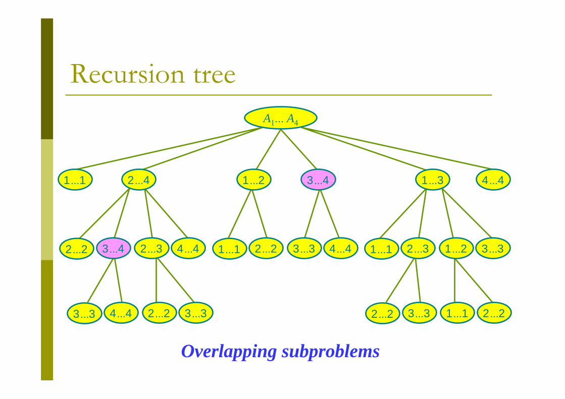
Recursion tree
1...1 2...2 3...3 4...42...2 3...4 2...3 4...4 1...1 2...3 1...2 3...3
3...3 4...4 2...2 3...3 2...2 3...3 1...1 2...2
2...41...1 3...41...2 4...41...3
A1... A4
Recursion tree
1...1 2...2 3...3 4...42...2 3...4 2...3 4...4 1...1 2...3 1...2 3...3
3...3 4...4 2...2 3...3 2...2 3...3 1...1 2...2
2...41...1 3...41...2 4...41...3
A1... A4
Overlapping subproblems

Recursion tree
1...1 2...2 3...3 4...42...2 3...4 2...3 4...4 1...1 2...3 1...2 3...3
3...3 4...4 2...2 3...3 2...2 3...3 1...1 2...2
2...41...1 3...41...2 4...41...3
A1... A4
Overlapping subproblems

Computing the optimal costsMatrix Dimension
A1 30 × 35A2 35 × 15A3 15 × 5A4 5 × 10A5 10 × 20A6 20 × 25
A1 A2 A3 A4 A5 A6
12
34
56 1
23
45
6
23
45
6 12
34
5
i
ij
s
m
j

Computing the optimal costsMatrix Dimension
A1 30 × 35A2 35 × 15A3 15 × 5A4 5 × 10A5 10 × 20A6 20 × 25
A1 A2 A3 A4 A5 A6
12
34
56 1
23
45
6
23
45
6 12
34
5
ij
ij
s
m
0 0 0 0 0 0

Computing the optimal costsMatrix Dimension
A1 30 × 35A2 35 × 15A3 15 × 5A4 5 × 10A5 10 × 20A6 20 × 25
A1 A2 A3 A4 A5 A6
12
34
56 1
23
45
6
23
45
6 12
34
5
ij
ij
s
m
0 0 0 0 0 0
15,750
m[1,2] = m[1,1] + m[2, 2] + p0 · p1 · p2
= 0 + 0 + 30 × 35 × 15= 15,750
1

Computing the optimal costsMatrix Dimension
A1 30 × 35A2 35 × 15A3 15 × 5A4 5 × 10A5 10 × 20A6 20 × 25
A1 A2 A3 A4 A5 A6
12
34
56 1
23
45
6
23
45
6 12
34
5
ij
ij
s
m
0 0 0 0 0 0
15,750
m[1,3] = min m[1,1] + m[2, 3] + p0 · p1 · p3m[1,2] + m[3, 3] + p0 · p2 · p3
= 7,875
1
7,875
2,625 750 1,000 5,000
2 3 4 5
1
= min 0 + 2,625 + 30 × 35 × 515,750 + 0 + 30 × 15 × 5
= min 7,87518,000

Computing the optimal costsMatrix Dimension
A1 30 × 35A2 35 × 15A3 15 × 5A4 5 × 10A5 10 × 20A6 20 × 25
A1 A2 A3 A4 A5 A6
12
34
56 1
23
45
6
23
45
6 12
34
5
ij
ij
s
m
0 0 0 0 0 0
15,750
m[2,5] = min m[2,2] + m[3, 5] + p1 · p2 · p5m[2,3] + m[4, 5] + p1 · p3 · p5m[2,4] + m[5, 5] + p1 · p4 · p5
= 7,125.
1
9,375 7,125
7,875 4,375 2,500 3,500
2,625 750 1,000 5,000
2 3 4 5
1 3 3 5
3 3
= min 0 + 2,500 + 30 × 15 × 202,625 +1,00 0 + 30 × 5 × 204,375 + 0 + 35 × 10 × 20
= min 13,0007,12511,375

Computing the optimal costsMatrix Dimension
A1 30 × 35A2 35 × 15A3 15 × 5A4 5 × 10A5 10 × 20A6 20 × 25
A1 A2 A3 A4 A5 A6
12
34
56 1
23
45
6
23
45
6 12
34
5
ij
ij
s
m
0 0 0 0 0 0
15,750
m[1,6] = 15,125
115,125
11,875 10,500
9,375 7,125 5,375
7,875 4,375 2,500 3,500
2,625 750 1,000 5,000
2 3 4 5
1 3 3 5
3 3 3
3 3
3

Constructing an optimal solutionMatrix Dimension
A1 30 × 35A2 35 × 15A3 15 × 5A4 5 × 10A5 10 × 20A6 20 × 25
A1 A2 A3 A4 A5 A6
12
34
56 1
23
45
6
23
45
6 12
34
5
ij
ij
s
m
0 0 0 0 0 0
15,750
m[1,6] = 15,125
115,125
11,875 10,500
9,375 7,125 5,375
7,875 4,375 2,500 3,500
2,625 750 1,000 5,000
2 3 4 5
1 3 3 5
3 3 3
3 3
3
(A1... A6) = ((A1... A3)(A4... A6 ))
= ((A1(A2 A3))(A4... A6 ))

Constructing an optimal solutionMatrix Dimension
A1 30 × 35A2 35 × 15A3 15 × 5A4 5 × 10A5 10 × 20A6 20 × 25
A1 A2 A3 A4 A5 A6
12
34
56 1
23
45
6
23
45
6 12
34
5
ij
ij
s
m
0 0 0 0 0 0
15,750
m[1,6] = 15,125
115,125
11,875 10,500
9,375 7,125 5,375
7,875 4,375 2,500 3,500
2,625 750 1,000 5,000
2 3 4 5
1 3 3 5
3 3 3
3 3
3
(A1... A6) = ((A1... A3)(A4... A6 ))
= ((A1(A2 A3))((A4A5)A6 ))
= ((A1(A2 A3))(A4... A6 ))

Elements of dynamic programmingOptimal substructure
Dynamic programming builds an optimal solution to theproblem from optimal solutions to subproblems.The solutions to the subproblems used within the optimalsolution to the problem must themselves be optimal by usinga "cut-and-paste" technique.Subproblems are independent.
Overlapping subproblemsRecursive algorithm revisits the same problem over and overagain.In contrast, a problem for which a divide-and-conquer approachis suitable usually generates brand-new problems at each stepof the recursion.

Divide-and-conquer algorithmIDEA:n × n matrix = 2 × 2 matrix of (n/2) × (n/2) submatrices:
r st u =
a bc d ·
e fg h
C = A · Br = ae + bgs = af + bht = ce + dgu = cf + dh
8 mults of (n/2) × (n/2) submatrices4 adds of (n/2) × (n/2) submatrices
recursive

Subtleties
Unweighted shortest path: Find a path from u to vconsisting the fewest edges.
Given a directed graph G = (V, E) and vertices u, v ∈ V.
Unweighted longest simple path: Find a path fromu to v consisting the most edges.
u r
s v
p1
p2
p3
p4
p5
p6
p7
p8

Subtleties
Unweighted shortest path: Find a path from u to vconsisting the fewest edges.
Given a directed graph G = (V, E) and vertices u, v ∈ V.
Unweighted longest simple path: Find a path fromu to v consisting the most edges.
u r
s v
Shortest path from u to v.u s v.
For intermediate vertex s.p1 and p2 must be shortest path.
p1
p2
p3
p4
p5
p6
p7
p81p 2p

Subtleties
Unweighted shortest path: Find a path from u to vconsisting the fewest edges.
Given a directed graph G = (V, E) and vertices u, v ∈ V.
Unweighted longest simple path: Find a path fromu to v consisting the most edges.
u r
s v
Longest path from u to v.u r v.
For intermediate vertex v.Is p8 longest simple path form uto r ?
p1
p2
p3
p4
p5
p6
p7
p88p 7p
No. It is u s v r1p 2p 3p

Subtleties
Unweighted shortest path: Find a path from u to vconsisting the fewest edges.
Given a directed graph G = (V, E) and vertices u, v ∈ V.
Unweighted longest simple path: Find a path fromu to v consisting the most edges.
u r
s v
Longest path from u to v.u r v.
For intermediate vertex v.Is p7 longest simple path form rto v ?
p1
p2
p3
p4
p5
p6
p7
p88p 7p
No. It is r u s v4p 1p 2p

Subtleties
Unweighted shortest path: Find a path from u to vconsisting the fewest edges.
Given a directed graph G = (V, E) and vertices u, v ∈ V.
Unweighted longest simple path: Find a path fromu to v consisting the most edges.
u r
s v
Longest path from u to v.u r v.
For intermediate vertex v. p1
p2
p3
p4
p5
p6
p7
p88p 7p
u s v4p 1p 2pu s v r1p 2p 3pCombine the longest simple paths
The path contains cycles and is not simple.

IndependentSubproblems in finding the longest simple path are not independent, whereas for shortest paths they are.Subproblems being independent means that the solution to one subproblem does not affect the solution to another subproblem.For longest simple path problem, we choose the first path u → s → v → r, and so we have also used the vertices s and t. We can no longer use these vertices in the second subproblem.Our use of resources in solving one subproblem has rendered them unavailable for the other subproblem.

Four steps of developmentCharacterize the structure of an optimal solution.Recursively define the value of an optimal solution.Compute the value of an optimal solution in a bottom-up fashion.Construct an optimal solution from computed information.

Longest Common SubsequenceGiven two sequences x[1 … m] and y[1 … n], find a longest subsequence common to them both.
x: A B C B D A B
y: B D C A B ABCBA = LCS(x, y)

Brute-force LCS algorithmCheck every subsequence of x[1 … m] to see if it is also a subsequence of y[1 … n].
AnalysisChecking = O(n) time per subsequence.2m subsequences of x (each bit-vector of length mdetermines a distinct subsequence of x).Worst-case running time = O(n2m)
= exponential time.
It is infeasible!

Optimal substructure of an LCSGiven a sequence W = <w1, w2, …, wn>, define the ithprefix of W, for i = 0, 1, …, m, as Wi = <w1, w2, …, wi>
Let X = <x1, x2, …, xm> and Y = <y1, y2, …, yn> be sequences, and let Z = <z1, z2, …, zk> be any LCS of Xand Y.
If xm = yn, then zk = xm = yn and Zk−1 is an LCS of Xm−1 and Yn−1.If xm ≠ yn, then zk ≠ xm and Z is an LCS of Xm−1 and Y.
If xm ≠ yn, then zk ≠ yn and Z is an LCS of X and Yn−1.

Recursive solutionLet us define c[i, j] to be the length of an LCS of the sequences Xi and Yj.The optimal substructure of the LCS problem gives the recursive formula.
c[i, j] =0 if i = 0 or j =0,c[i − 1, j − 1] + 1 if i, j > 0 and xi = yj,max(c[i, j − 1], c[i − 1, j]) if i, j > 0 and xi ≠ yj.
1 2 mi
1 2 nj=
X:
Y: Our goal is c[m, n]

Computing LCS
xi
ABCBDAB
yj B D C A B A0
12
34
5
67
0 1 2 3 4 5 6jci

Computing LCS
xi
ABCBDAB
yj B D C A B A0
12
34
5
67
0 1 2 3 4 5 6ji
0 0 0 0 0 0 0
0
0
0
0
0
0
0
c

Computing LCS
xi
ABCBDAB
yj B D C A B A0
12
34
5
67
0 1 2 3 4 5 6ji
0 0 0 0 0 0 0
0
0
0
0
0
0
0
c
0
x1 ≠ y1 andc[0, 1] ≥ c[1, 0] then c[1, 1] = c[0, 1]

Computing LCS
xi
ABCBDAB
yj B D C A B A0
12
34
5
67
0 1 2 3 4 5 6ji
0 0 0 0 0 0 0
0
0
0
0
0
0
0
c
0
x1 = y4 thenc[1, 4] = c[0, 3] + 1
0 0 1

Computing LCS
xi
ABCBDAB
yj B D C A B A0
12
34
5
67
0 1 2 3 4 5 6ji
0 0 0 0 0 0 0
0
0
0
0
0
0
0
c
0
x1 ≠ y5 thenc[0, 5] < c[1, 4] then c[1, 5] = c[1, 4]
0 0 1 1

Computing LCS
xi
ABCBDAB
yj B D C A B A0
12
34
5
67
0 1 2 3 4 5 6ji
0 0 0 0 0 0 0
0
0
0
0
0
0
0
c
0 0 0 1 1 1
1 1 1 1 2 2
1 1
21
1
1
1
2 2 2 2
1 2 3 3
22 3
2 2
2 2 2 3 3
3
3 4
4
4
x7 ≠ y6 andc[6, 6] ≥ c[7, 5] then c[7, 6] = c[6, 6]

Constructing an LCS
xi
ABCBDAB
yj B D C A B A0
12
34
5
67
0 1 2 3 4 5 6ji
0 0 0 0 0 0 0
0
0
0
0
0
0
0
c
0
c[7, 6] = 4 andLCS(X, Y) = BCBA
0 0 1 1 1
1 1 1 1 2 2
1 1
21
1
1
1
2 2 2 2
1 2 3 3
22 3
2 2
2 2 2 3 3
3
3 4
4
4

Any question?Xiaoqing Zheng
Fundan University
Top Related