


Languages
Pages
Legal

Data Hiding in Digital Images : A SteganographicParadigm
A thesis submitted in Partial Fulfillment of
the requirements for the Award of the degree of
Master of Technology
in
Computer Science and Engineering
by
Piyush Goel(Roll No. 03CS3003)
Under the guidance of
Prof. Jayanta Mukherjee
Department of Computer Science & Engineering
Indian Institute of Technology–Kharagpur
May, 2008

Certificate
This is to certify that the thesis titled Data Hiding in Digital Images : A Steganographic
Paradigm submitted by Piyush Goel, Roll No. 03CS3003, to the Department of Computer
Science and Engineering in partial fulfillment of the requirements of the degree of Master of
Technology in Computer Science and Engineering is a bonafide record of work carried out
by him under my supervision and guidance. The thesis has fulfilled all the requirements as per
the rules and regulations of this Institute and, in my opinion, has reached the standard needed
for submission.
Prof. Jayanta Mukherjee
Dept. of Computer Science and Engineering
Indian Institute of Technology
Kharagpur 721302, INDIA
May 2008

Acknowledgments
It is with great reverence that I wish to express my deep gratitude towards Prof. Jayanta
Mukherjee for his astute guidance, constant motivation and trust, without which this work would
never have been possible. I am sincerely indebted to him for his constructive criticism and
suggestions for improvement at various stages of the work.
I would also like to thank Mr. Arijit Sur, Research Scholar, for his guidance, invaluable
suggestions and for bearing with me during the thought provoking discussions which made this
work possible. I am grateful to Prof. Arun K. Majumdar for his guidance and the stimulating
discussions during the last semester. I am also thankful to Prof. Andreas Westfeld, Technical
University of Dresden, Germany, for clearing some of my doubts through email.
I am grateful to my parents and brother for their perennial inspiration.
Last but not the least, I would like to thank all my seniors, wingmates and my batchmates
especially Mayank, Udit , Joydeep , Prithvi, Lalit, Arpit, Sankalp, Mukesh, Amar and Umang
for making my stay at IIT Kharagpur comfortable and a fruitful learning experience.
Date: Piyush Goel
Abstract
In this thesis a study on the Steganographic paradigm of data hiding has been presented.
The problem of data hiding has been attacked from two directions. The first approach tries to
overcome the Targeted Steganalytic Attacks. The work focuses mainly on the first order statis-
tics based targeted attacks. Two algorithms have been presented which can preserve the first
order statistics of an image after embedding. Experimental Results reveal that preserving the
image statistics using the proposed algorithm improves the security of the algorithms against the
targeted attacks. The second approach aims at resisting Blind Steganalytic Attacks especially
the Calibration based Blind Attacks which try to estimate a model of the cover image from the
stego image. A Statistical Hypothesis Testing framework has been developed for testing the
efficiency of a blind attack. A generic framework for JPEG steganography has been proposed
which disturbs the cover image model estimation of the blind attacks. This framework has also
been extended to a novel steganographic algorithm which can be used for any JPEG domain
embedding scheme. Experimental results show that the proposed algorithm can successfully
resist the calibration based blind attacks and some non-calibration based attacks as well.
iii

Contents
Abstract iii
List of Tables vi
List of Figures vii
1 Introduction 1
1.1 Steganography . . . . . . . . . . . . . . . . . . . . . . . . . . . . . . . . . . 1
1.2 A Steganographic Framework . . . . . . . . . . . . . . . . . . . . . . . . . . 4
1.3 Organization of the Thesis . . . . . . . . . . . . . . . . . . . . . . . . . . . . 5
2 Literature Survey 7
2.1 Existing Steganographic Techniques . . . . . . . . . . . . . . . . . . . . . . . 7
2.1.1 Spatial Domain . . . . . . . . . . . . . . . . . . . . . . . . . . . . . . 7
2.1.2 Transform Domain . . . . . . . . . . . . . . . . . . . . . . . . . . . . 9
2.2 Existing Attacks . . . . . . . . . . . . . . . . . . . . . . . . . . . . . . . . . . 10
2.2.1 Targeted Attacks . . . . . . . . . . . . . . . . . . . . . . . . . . . . . 10
2.2.2 Blind Attacks . . . . . . . . . . . . . . . . . . . . . . . . . . . . . . . 12
2.3 Summary . . . . . . . . . . . . . . . . . . . . . . . . . . . . . . . . . . . . . 14
3 Statistical Restoration 15
3.1 Introduction . . . . . . . . . . . . . . . . . . . . . . . . . . . . . . . . . . . . 16
3.2 Embedding by Pixel Swapping . . . . . . . . . . . . . . . . . . . . . . . . . . 17
3.2.1 Algorithm Pixel Swap Embedding . . . . . . . . . . . . . . . . . . . . 17
3.2.2 Security Analysis . . . . . . . . . . . . . . . . . . . . . . . . . . . . . 20
3.3 New Statistical Restoration Scheme . . . . . . . . . . . . . . . . . . . . . . . 20
iv
3.3.1 Mathematical Formulation of Proposed Scheme . . . . . . . . . . . . . 22
3.3.2 Algorithm Statistical Restoration . . . . . . . . . . . . . . . . . . . . . 24
3.3.3 Restoration with Minimum Distortion . . . . . . . . . . . . . . . . . . 25
3.3.4 Experimental Results . . . . . . . . . . . . . . . . . . . . . . . . . . . 26
3.3.5 Security Analysis . . . . . . . . . . . . . . . . . . . . . . . . . . . . . 26
3.4 Summary . . . . . . . . . . . . . . . . . . . . . . . . . . . . . . . . . . . . . 34
4 Spatial Desynchronization 35
4.1 Introduction . . . . . . . . . . . . . . . . . . . . . . . . . . . . . . . . . . . . 35
4.2 Calibration Attack . . . . . . . . . . . . . . . . . . . . . . . . . . . . . . . . . 37
4.2.1 23 Dimensional Calibration Attack . . . . . . . . . . . . . . . . . . . 37
4.2.2 274 Dimensional Calibration Attack . . . . . . . . . . . . . . . . . . . 37
4.2.3 Statistical Test for Calibration Attack . . . . . . . . . . . . . . . . . . 38
4.3 Counter Measures to Blind Steganalysis . . . . . . . . . . . . . . . . . . . . . 43
4.3.1 Spatial Block Desynchronization . . . . . . . . . . . . . . . . . . . . . 45
4.4 The Proposed Algorithm . . . . . . . . . . . . . . . . . . . . . . . . . . . . . 47
4.4.1 Spatially Desynchronized Steganographic Algorithm (SDSA) . . . . . 47
4.4.2 Hypothesis Testing . . . . . . . . . . . . . . . . . . . . . . . . . . . . 49
4.5 Experiments and Results . . . . . . . . . . . . . . . . . . . . . . . . . . . . . 51
4.6 Summary . . . . . . . . . . . . . . . . . . . . . . . . . . . . . . . . . . . . . 53
5 Conclusions and Future Directions 54
5.1 Conclusions . . . . . . . . . . . . . . . . . . . . . . . . . . . . . . . . . . . . 54
5.2 Future Directions . . . . . . . . . . . . . . . . . . . . . . . . . . . . . . . . . 55
v

List of Tables
4.1 p value of the Rank-Sum Test for 23 DCA and 274 DCA . . . . . . . . . . . . 40
4.2 p value of the Rank-Sum Test for 274 DCA for testing the Self Calibration Process 41
4.3 p-value of Rank Sum Test for 23 DCA . . . . . . . . . . . . . . . . . . . . . . 50
4.4 p-value of Rank Sum Test for 274 DCA . . . . . . . . . . . . . . . . . . . . . 50
4.5 Area under ROC for QIM, YASS and SDSA against 23 DCA . . . . . . . . . . 52
4.6 Detection Accuracy of QIM, YASS and SDSA against 23 DCA . . . . . . . . 52
4.7 Area under ROC for QIM, YASS and SDSA against Farid’s 92 Dimensional
Attack . . . . . . . . . . . . . . . . . . . . . . . . . . . . . . . . . . . . . . . 53
4.8 Detection Accuracy of QIM, YASS and SDSA against Farid’s 92 Dimensional
Attack . . . . . . . . . . . . . . . . . . . . . . . . . . . . . . . . . . . . . . . 53
vi

List of Figures
1.1 Tradeoff between embedding capacity, undetectability and robustness in data
hiding. . . . . . . . . . . . . . . . . . . . . . . . . . . . . . . . . . . . . . . . 3
1.2 Visual attacks for detecting hidden messages in an image layer . . . . . . . . . 3
1.3 A generalized steganographic framework . . . . . . . . . . . . . . . . . . . . 4
1.4 Framework for Private Key Passive Warden Steganography. . . . . . . . . . . . 5
2.1 Flipping of set cardinalities during embedding . . . . . . . . . . . . . . . . . . 11
2.2 Calibration of the stego image for cover statistics estimation . . . . . . . . . . 13
3.1 PSNR for the Pixel Swap Embedding Algorithm for different values of ε. . . . 19
3.2 Maximum Achievable Embedding Rates for PSE Algorithm for different values
of ε. . . . . . . . . . . . . . . . . . . . . . . . . . . . . . . . . . . . . . . . . 21
3.3 Result of testing PSE algorithm against Sample Pair Attack for ε = 5. . . . . . . 22
3.4 Sample Test Images . . . . . . . . . . . . . . . . . . . . . . . . . . . . . . . . 27
3.5 Results for Dinosaur . . . . . . . . . . . . . . . . . . . . . . . . . . . . . . . 28
3.6 Results for Baboon . . . . . . . . . . . . . . . . . . . . . . . . . . . . . . . . 29
3.7 Results for Hills . . . . . . . . . . . . . . . . . . . . . . . . . . . . . . . . . . 30
3.8 Scatter Plot showing amount of reduction in difference histogram using SRA
algorithm and Solanki’s Scheme . . . . . . . . . . . . . . . . . . . . . . . . . 31
3.9 ROC plot of Sample pair steganalysis on SRA scheme with an average embed-
ding rate of 0.25 bpp . . . . . . . . . . . . . . . . . . . . . . . . . . . . . . . 31
3.10 Comparison of SRA algorithm and Solanki’s scheme against Sample Pair Attack 32
3.11 ROC plot of WAM steganalysis on SRA algorithm and Solanki’s scheme with
an average embedding rate of 0.125 bpp . . . . . . . . . . . . . . . . . . . . . 33
4.1 L2 Norms of Cover/Stego and Cropped Cover/Cropped Stego 1 . . . . . . . . . 42
vii

4.2 L2 Norms of Cover/Stego and Cropped Cover/Cropped Stego 2 . . . . . . . . . 44
4.3 Block Diagram of Spatial Block Desynchronization . . . . . . . . . . . . . . . 46
4.4 Block Diagram of Proposed Method . . . . . . . . . . . . . . . . . . . . . . . 47
viii
Chapter 1
Introduction
1.1 Steganography
Steganography is the art of hiding information imperceptibly in a cover medium. The word
”Steganography” is of Greek origin and means ”covered or hidden writing”. The main aim in
steganography is to hide the very existence of the message in the cover medium. Steganography
includes a vast array of methods of secret communication that conceal the very existence of
hidden information. Traditional methods include use of invisible inks, microdots etc. Modern
day steganographic techniques try to exploit the digital media images, audio files, video files
etc
Steganography and cryptography are cousins in the spy craft family. Cryptography scram-
bles a message by using certain cryptographic algorithms for converting the secret data into
unintelligible form. On the other hand, Steganography hides the message so that it cannot be
seen. A message in cipher text might arouse suspicion on the part of the recipient while an
”invisible” message created with steganographic methods will not. Anyone engaging in secret
communication can always apply a cryptographic algorithm to the data before embedding it to
achieve additional security. In any case, once the presence of hidden information is revealed
or even suspected, the purpose of steganography is defeated, even if the message content is not
extracted or deciphered. According to [1] , “Steganography’s niche in security is to supplement
cryptography, not replace it. If a hidden message is encrypted, it must also be decrypted if
discovered, which provides another layer of protection.”
1

Another form of data hiding in digital images is Watermarking. Digital watermarking
is the process of embedding auxiliary information into a digital cover signal with the aim of
providing authentication information. A watermark is called robust with respect to a class of
transformations if the embedded information can reliably be detected from the marked signal
even if degraded by any transformation within that class. Typical image degradations are JPEG
compression, rotation, cropping, additive noise and quantization.
Steganography and watermarking differ in a number of ways including purpose, specifi-
cation and detection/extraction methods. The most fundamental difference is that the object of
communication in watermarking is the host signal, with the embedded data providing copyright
protection. In steganography the object to be transmitted is the embedded message, and the
cover signal serves as an innocuous disguise chosen fairly arbitrarily by the user based on its
technical suitability. In addition, the existence of the watermark is often declared openly, and
any attempt to remove or invalidate the embedded content renders the host useless. The crucial
requirement for steganography is perpetual and algorithmic undetectability. Robustness against
malicious attack and signal processing is not the primary concern, as it is for watermarking. The
difference between Steganography and Watermarking with respect the three parameters of pay-
load, undetectability and robustness can be understood from Figure 1.1.
As mentioned, steganography deals with hiding of information in some cover source. On
the other hand, Steganalysis is the art and science of detecting messages hidden using steganog-
raphy; this is analogous to cryptanalysis applied to cryptography. The goal of steganalysis is to
identify suspected packages, determine whether or not they have a payload encoded into them,
and, if possible, recover that payload. Hence, the major challenges of effective steganography
are:-
1. Security of Hidden Communication: In order to avoid raising the suspicions of eaves-
droppers, while evading the meticulous screening of algorithmic detection, the hidden
contents must be invisible both perceptually and statistically.
2. Size of Payload: Unlike watermarking, which needs to embed only a small amount of
copyright information, steganography aims at hidden communication and therefore usu-
ally requires sufficient embedding capacity. Requirements for higher payload and secure
communication are often contradictory. Depending on the specific application scenarios,
a trade off has to be sought.
2

Figure 1.1: Tradeoff between embedding capacity, undetectability and robustness in data hiding.
One of the possible ways of categorizing the present steganalytic attacks is on the follow-
ing two categories :
Figure 1.2: Visual attacks for detecting hidden messages in an image layer
1. Visual Attacks: These methods try to detect the presence of information by visual in-
spection either by the naked eye or by a computer. The attack is based on guessing the
embedding layer of an image (say a bit plane) and then visually inspecting that layer to
look for any unusual modifications in that layer as shown in Figure 1.2.
2. Statistical Attacks: These methods use first or higher order statistics of the image to
reveal tiny alterations in the statistical behavior caused by steganographic embedding and
3
hence can successfully detect even small amounts of embedding with very high accuracy.
These class of steganalytic attacks are further classified as ’Targeted Attacks’ or ’Blind
Attacks’ as explained in detail in the next few sections.
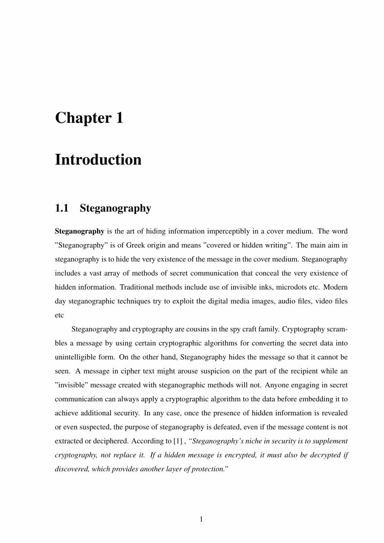
Figure 1.3: A generalized steganographic framework
1.2 A Steganographic Framework
Any steganographic system can be studied as shown in Figure 1.3. For a steganographic al-
gorithm having a stego-key, given any cover image the embedding process generates a stego
image. The extraction process takes the stego image and using the shared key applies the in-
verse algorithm to extract the hidden message.
This system can be explained using the ’prisoners problem’ (Figure 1.4) where Alice and
Bob are two inmates who wish to communicate in order to hatch an escape plan. However
communication between them is examined by the warden, Wendy. To send the secret message
to Bob, Alice embeds the secret message ’m’ into the cover object ’c’, to obtain the stego
object ’s’. The stego object is then sent through the public channel. In a pure steganographic
framework, the technique for embedding the message is unknown to Wendy and shared as a
secret between Alice and Bob. In private key steganography Alice and Bob share a secret key
which is used to embed the message. The secret key, for example, can be a password used to
seed a pseudo-random number generator to select pixel locations in an image cover-object for
embedding the secret message. Wendy has no knowledge about the secret key that Alice and
4

Bob share, although she is aware of the algorithm that they could be employing for embedding
messages. In public key steganography, Alice and Bob have private-public key pairs and know
each other’s public key. In this thesis we confine ourselves to private key steganography only.
Figure 1.4: Framework for Private Key Passive Warden Steganography.
1.3 Organization of the Thesis
This thesis is organized as follows : In Chapter 2, “Literature Survey”, we give a background
of the existing state of the steganographic research. We cover briefly the main categories of
steganographic algorithms covered till date although the survey is not exhaustive and we may
have missed out some of the algorithms. We also present a survey on the two categories of Ste-
ganalytic Attacks, “Targeted” and “Blind” and briefly describe the attacks especially the attacks
that are relevant to this thesis. In Chapter 3, “Statistical Restoration”, we present the motiva-
tion for working on this approach in steganography and present some of the existing algorithms
based on this approach. We introduce two new algorithms for data embedding with statistical
preservation and make a comparative analysis of the proposed algorithms with the existing ones.
In Chapter 4, “Spatial Desynchronization”, we first study the calibration based blind attacks and
analyze two of the existing attacks using a novel Statistical Hypothesis Testing Framework to
test their effectiveness against steganographic embedding. We introduce a new framework for
JPEG steganographic algorithms called “Spatial Desynchronization” and extend this framework
to a new steganographic scheme called “Spatially Desynchronized Steganographic Algorithm”.
We make a comparative analysis of the proposed algorithm with the existing techniques with
5
respect to the statistical hypothesis testing framework introduced in the same chapter and also
with respect to two more metrics of evaluation (Area under ROC, Detection Accuracy). The
thesis is concluded in Chapter 5 with the concluding remarks. We also try to identify and
present some avenues of future research. Also, the papers included in the bibliography and the
source code of all the algorithms and attacks implemented in the course of this work have been
attached in the form of a CD with the thesis.
6
Chapter 2
Literature Survey
In this chapter we provide the necessary background required for this thesis. In section 2.1
we discuss briefly some of the existing steganographic techniques. In section 2.2 we present
some of the steganalytic attacks proposed till date as a counter measure to the steganographic
algorithms.
2.1 Existing Steganographic Techniques
The steganographic algorithms proposed in literature can broadly be classified into two cate-
gories.
1. Spatial Domain Techniques
2. Transform Domain Techniques
Each of these techniques are covered in detail in the next two subsections.
2.1.1 Spatial Domain
These techniques use the pixel gray levels and their color values directly for encoding the mes-
sage bits. These techniques are some of the simplest schemes in terms of embedding and extrac-
tion complexity. The major drawback of these methods is amount of additive noise that creeps
in the image which directly affects the Peak Signal to Noise Ratio and the statistical properties
of the image. Moreover these embedding algorithms are applicable mainly to lossless image
7

compression schemes like TIFF images. For lossy compression schemes like JPEG, some of
the message bits get lost during the compression step.
The most common algorithm belonging to this class of techniques is the Least Significant
Bit (LSB) Replacement technique in which the least significant bit of the binary representation
of the pixel gray levels is used to represent the message bit. This kind of embedding leads to an
addition of a noise of 0.5p on average in the pixels of the image where p is the embedding rate
in bits/pixel. This kind of embedding also leads to an asymmetry and a grouping in the pixel
gray values (0,1);(2,3);. . . (254,255). This asymmetry is exploited in the attacks developed for
this technique as explained further in section 2.2. To overcome this undesirable asymmetry, the
decision of changing the least significant bit is randomized i.e. if the message bit does not match
the pixel bit, then pixel bit is either increased or decreased by 1. This technique is popularly
known as LSB Matching. It can be observed that even this kind of embedding adds a noise of
0.5p on average. To further reduce the noise, [2] have suggested the use of a binary function
of two cover pixels to embed the data bits. The embedding is performed using a pair of pixels
as a unit, where the LSB of the first pixel carries one bit of information, and a function of the
two pixel values carries another bit of information. It has been shown that embedding in this
fashion reduces the embedding noise introduced in the cover signal.
In [4], a multiple base number system has been employed for embedding data bits. While
embedding, the human vision sensitivity has been taken care of. The variance value for a block
of pixels is used to compute the number base to be used for embedding. A similar kind of
algorithm based on human vision sensitivity has been proposed by [5] by the name of Pixel
Value Differencing. This approach is based on adding more amount of data bits in the high
variance regions of the image for example near “the edges” by considering the difference values
of two neighboring pixels. This approach has been improved further by clubbing it with least
significant bit embedding in [6].
According to [20], “For a given medium, the steganographic algorithm which makes fewer
embedding changes or adds less additive noise will be less detectable as compared to an algo-
rithm which makes relatively more changes or adds higher additive noise.” Following the same
line of thought Crandall [7] have introduced the use of an Error Control Coding technique called
“Matrix Encoding”. In Matrix Encoding, q message bits are embedded in a group of 2q − 1
cover pixels while adding a noise of 1 − 2−q per group on average. The maximum embedding
capacity that can be achieved is q2q−1
. For example, 2 bits of secret message can be embedded
8
in a group of 3 pixels while adding a noise of 0.75 per group on average. The maximum em-
bedding capacity achievable is 2/3 = 0.67 bits/pixel. F5 algorithm [17] is probably the most
popular implementation of Matrix Encoding.
LSB replacement technique has been extended to multiple bit planes as well. Recently
[3] has claimed that LSB replacement involving more than one least significant bit planes is
less detectable than single bit plane LSB replacement. Hence the use of multiple bit planes for
embedding has been encouraged. But the direct use of 3 or more bit planes leads to addition
of considerable amount of noise in the cover image. [8] and [9] have given a detailed analysis
of the noise added by the LSB embedding in 3 bit planes. Also, a new algorithm which uses a
combination of Single Digit Sum Function and Matrix Encoding has been proposed. It has been
shown analytically that the noise added by the proposed algorithm in a pixel of the image is
0.75p as compared to 0.875p added by 3 plane LSB embedding where p is the embedding rate.
One point to be observed here is that most of the approaches proposed so far are based
on minimization of the noise embedded in the cover by the algorithm. Another direction of
steganographic algorithm is preserving the statistics of the image which get changed due to
embedding. Chapter 2 of this thesis proposes two algorithms based on this approach itself. In
the next section we cover some of the transform domain steganographic algorithms.
2.1.2 Transform Domain
These techniques try to encode message bits in the transform domain coefficients of the image.
Data embedding performed in the transform domain is widely used for robust watermarking.
Similar techniques can also realize large-capacity embedding for steganography. Candidate
transforms include discrete cosine Transform (DCT), discrete wavelet transform (DWT), and
discrete Fourier transform (DFT). By being embedded in the transform domain, the hidden
data resides in more robust areas, spread across the entire image, and provides better resistance
against signal processing. For example, we can perform a block DCT and, depending on pay-
load and robustness requirements, choose one or more components in each block to form a new
data group that, in turn, is pseudo randomly scrambled and undergoes a second-layer trans-
formation. Modification is then carried out on the double transform domain coefficients using
various schemes. These techniques have high embedding and extraction complexity. Because
of the robustness properties of transform domain embedding, these techniques are generally
more applicable to the “Watermarking” aspect of data hiding. Many steganographic techniques
9

in these domain have been inspired from their watermarking counterparts.
F5 [17] uses the Discrete Cosine Transform coefficients of an image for embedding data
bits. F5 embeds data in the DCT coefficients by rounding the quantized coefficients to the
nearest data bit. It also uses Matrix Encoding for reducing the embedded noise in the signal. F5
is one the most popular embedding schemes in DCT domain steganography, though it has been
successfully broken in [42].
The transform domain embedding does not necessarily mean generating the transform
coefficients on a blocks of size 8 × 8 as done in JPEG compression techniques. It is possible
to design techniques which take the transforms on the whole image [10]. Other block based
JPEG domain and wavelet based embedding algorithms have been proposed in [11] and [25]
respectively.
2.2 Existing Attacks
The steganalytic attacks developed till date can be classified into visual and statistical attacks.
The statistical attacks can further be classified as
1. Targeted Attacks
2. Blind Attacks
Each of these classes of attack is covered in detail in the next two subsections along with
several examples of each category.
2.2.1 Targeted Attacks
These attacks are designed keeping a particular steganographic algorithm in mind. These attacks
are based on the image features which get modified by a particular kind of steganographic
embedding. A particular steganographic algorithm imposes a specific kind of behaviour on
the image features. This specific kind of behaviour of the image statistics is exploited by the
targeted attacks. Some of the targeted attacks are as follows:
1. Histogram Analysis: The histogram analysis method exploits the asymmetry introduced
by LSB replacement. The main idea is to look for statistical artifacts of embedding in
the histogram of a given image. It has been observed statistically that in natural images
10
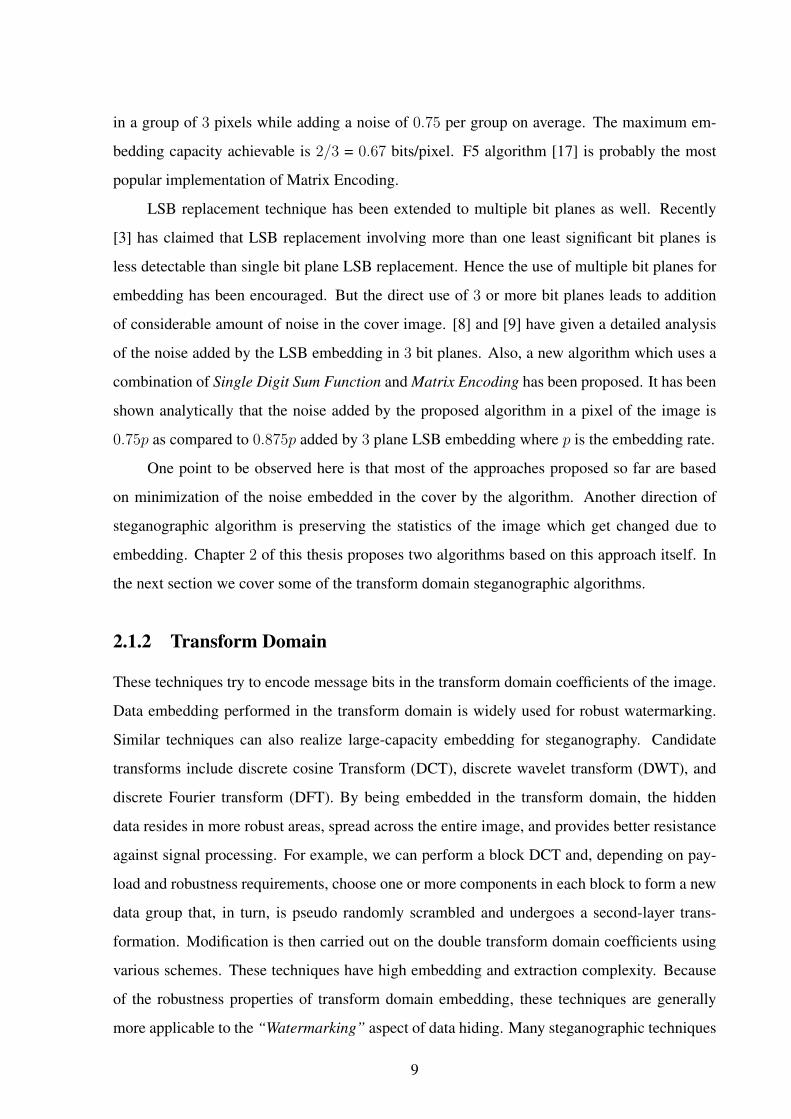
Figure 2.1: Flipping of set cardinalities during embedding
(cover images), the number of odd pixels and the number of even pixels are not equal.
For higher embedding rates of LSB Replacement these quantities tend to become equal.
So, based on this artifact a statistical attack based on the Chi-Square Hypothesis Testing
is developed to probabilistically suggest one of the following two hypothesis:
Null Hypothesis H0: The given image contains steganographic embedding
Alternative HypothesisH1: The given image does not contain steganographic embedding
The decision to accept or reject the Null Hypothesis H0 is made on basis of the observed
confidence value p. A more detailed discussion on Histogram Analysis can be found in
[37].
2. Sample Pair Analysis : Sample Pair Analysis is another LSB steganalysis technique
that can detect the existence of hidden messages that are randomly embedded in the least
significant bits of natural continuous-tone images. It can precisely measure the length of
the embedded message, even when the hidden message is very short relative to the image
size. The key to this methods success is the formation of 4 subsets of pixels (X , Y , U ,
and V ) whose cardinalities change with LSB embedding (as shown in Figure 2.1), and
such changes can be precisely quantified under the assumption that the embedded bits are
randomly scattered. A detailed analysis on Sample Pair technique can be found in [34].
Another attack called RS Steganalysis based on the same concept has been independently
proposed by [38].
11

3. HCF-COM based Attack: This attack first proposed by [43] is based on the Center of
Mass (COM) of the Histogram Characteristic Function (HCF) of an image. This attack
was further extended for LSB Matching by [39]. This attack observes the COM of a
cover/stego image (C(HC)/C(HS)) and its calibrated version obtained by down sampling
the image (C(HC)/C(HS)). It has been proved empirically that :
C(HC) ≈ C(HC) (2.1)
C(HC)− C(HS) > C(HC)− C(HS) (2.2)
From Equations 2.1 and 2.2, a dimensionless discriminator for classification can be ob-
tained as C(HS)C(HS)
. By estimating suitable threshold values of the discriminator from a set
of training data, an image can be classified either as cover or stego.
Some other targeted attacks also exist in literature which have not been covered in this
survey. A detailed survey can be found in [35]
2.2.2 Blind Attacks
The blind approach to steganalysis is similar to the pattern classification problem. The pattern
classifier, in our case a Binary Classifier, is trained on a set of training data. The training data
comprises of some high order statistics of the transform domain of a set of cover and stego
images and on the basis of this trained dataset the classifier is presented with images for classi-
fication as a non-embedded or an embedded image. Many of the blind steganalytic techniques
often try to estimate the cover image statistics from stego image by trying to minimize the effect
of embedding in the stego image. This estimation is sometimes referred to as “Cover Image
Prediction”. Some of the most popular blind attacks are defined next.
1. Wavelet Moment Analysis (WAM): Wavelet Moment Analyzer (WAM) is the most pop-
ular Blind Steganalyzer for Spatial Domain Embedding. It has been proposed by [40].
WAM uses a denoising filter to remove Gaussian noise from images under the assump-
tion that the stego image is an additive mixture of a non-stationary Gaussian signal (the
cover image) and a stationary Gaussian signal with a known variance (the noise). As the
12

Figure 2.2: Calibration of the stego image for cover statistics estimation
filtering is performed in the wavelet domain, all the features (statistical moments) are cal-
culated as higher order moments of the noise residual in the wavelet domain. The detailed
procedure for calculating the WAM features in a gray scale image can be found in [40].
WAM is based on a 27 dimension feature space. It then uses a Fisher Linear Discriminant
(FLD) as a classifier. It must be noted that WAM is a state of the art steganalyzer for
Spatial Domain Embedding and no other blind attack has been reported which performs
better than WAM.
2. Calibration Based Attacks: The calibration based attacks estimate the cover image
statistics by nullifying the impact of embedding in the cover image. These attacks were
first proposed by [14] and are designed for JPEG domain steganographic schemes. They
estimate the cover image statistics by a process termed as Self Calibration. The ste-
ganalysis algorithms based on this self calibration process can detect the presence of
steganographic noise with almost 100% accuracy even for very low embedding rates
[14, 28]. This calibration is done by decompressing the stego JPEG image to spatial
domain and cropping 4 rows from the top and 4 columns from the left and recompressing
the cropped image as shown in Figure 2.2. The cropping and subsequent recompres-
sion produce a “calibrated” image with most macroscopic features similar to the original
cover image. The process of cropping by 4 pixels is an important step because the 8 × 8
grid of recompression “does not see” the previous JPEG compression and thus the ob-
tained DCT coefficients are not influenced by previous quantization (and embedding) in
the DCT domain. The details of these attacks are covered in Chapter 4.
3. Farid’s Wavelet Based Attack: This attack was one of the first blind attacks to be pro-
posed in steganographic research [13] for JPEG domain steganography. It is based on the
13

features drawn from the wavelet coefficients of an image. This attack first makes an n
level wavelet decomposition of an image and computes four statistics namely Mean, Vari-
ance, Skewness and Kurtosis for each set of coefficients yielding a total of 12 × (n − 1)
coefficients. The second set of statistics is based on the errors in an optimal linear predic-
tor of coefficient magnitude. It is from this error that additional statistics i.e. the mean,
variance, skewness, and kurtosis are extracted thus forming a 24 × (n − 1) dimensional
feature vector. For implementation purposes, n is set to 4 i.e. four level decomposition
on the image is performed for extraction of features. The source code of this attack is
available at [32]. After extraction of features, a Support Vector Machine (SVM) is used
for classification. We would like to mention that although in [32] a SVM has been used
for classification we have used the Linear Discriminant Analysis for classification.
Some other blind attacks have also been proposed in literature. [30] have modeled the
difference between absolute value of neighboring DCT coefficients as a Markov process to
extract 324 features for classifying images as cover or stego. [28] have extended the features of
[14] to 193 and clubbed them with 72 features derived by reducing the 324 extracted by [30].
2.3 Summary
In this chapter, we have covered some of the necessary background needed for the rest of the
thesis. Some other concepts and definitions may be used from time to time and they shall be
explained as and when needed.
14
Chapter 3
Statistical Restoration
Statistical undetectability is one of the main aspects of any steganographic algorithm. To main-
tain statistical undetectability, the steganographic techniques are designed with the aim of min-
imizing the artifacts introduced in the cover signal by the embedding technique. The main
emphasis is generally on minimizing the noise added by embedding while increasing the pay-
load. This is an important consideration in the design of embedding algorithms, since the noise
added effects the statistical properties of a medium. As already mentioned previously, the al-
gorithm which makes fewer embedding changes or adds less additive noise generally provides
better security than the algorithm which makes relatively more changes or adds higher additive
noise [33].
From the point of view of the steganalyst, the attacks are designed to examine a signal and
look for statistics which get distorted due to embedding. These statistics range from marginal
statistics of first and second order in case of targeted attacks[34, 38, 39] and upto 9th order
statistics for blind attacks [40]. So, in order to defeat these steganalytic attacks, there has been
a shift from the above mentioned data hiding paradigm. Algorithms have been proposed which
try to restore the statistics which get distorted during the embedding procedure and are used for
steganalysis.
In this chapter we review some of the existing schemes based on this approach of pre-
serving the marginal statistics of an image in section 3.1. In section 3.2 we propose a new
algorithm which inherently preserves the first order statistics of the cover image during embed-
ding. In section 3.3, a steganographic method is proposed which explicitly preserves the first
order statistics during embedding. We provide experimental results to show that the two pro-
posed schemes give better performance than existing restoration methods. The chapter is finally
15
concluded in section 3.4.
3.1 Introduction
In steganographic research several algorithms have been proposed for preserving statistical fea-
tures of the cover for achieving more security. Provos’ Outguess algorithm [18] was an early
attempt at histogram compensation for LSB hiding, while Eggers et al [41] have suggested a
more rigorous approach to the same end, using histogram-preserving data-mapping (HPDM)
and adaptive embedding respectively.
Solanki et al [21, 22] have proposed a statistical restoration method for converting the
stego image histogram into the cover histogram. This algorithm is based on a theorem proved
by [36] which tries to convert one vector x into another vector y while satisfying a Minimum
Mean Square Error (MMSE) criterion. The algorithm considers the stego image histogram as
source vector x and tries to convert it into the cover image histogram i.e. the target vector y.
All the bins of the source histogram are compensated by mapping the input data with values in
increasing order. This algorithm suffers from the following limitations:
1. The algorithm assumes the cover image to be a Gaussian cover and does not give good
results for non-Gaussian cover images.
2. The algorithm ignores low probability image regions for embedding due to erratic behav-
ior in low probability tail.
3. The algorithm has been tried specifically for Quantization Index Modulation algorithm
[23] and it has not been tested for some well known embedding schemes like LSB Re-
placement, LSB matching etc.
To overcome the above limitations we propose two algorithms for preserving the cover
image statistics after embedding. The first algorithm is designed to inherently preserve the first
order statistics during embedding itself. The algorithm makes an explicit attempt at restoring
the cover image histogram after embedding. These algorithms are discussed in detail in the next
two sections.
16

3.2 Embedding by Pixel Swapping
The main motivation the steganographic algorithm proposed in this section is to embed data
such that the histogram of the image does not get modified. Such a requirement entails an
embedding procedure which does not modify the pixel values such that the corresponding bin
value in the histogram is changed. We propose a simple yet effective algorithm called “Pixel
Swap Embedding” which embeds message bits into the cover image without making any mod-
ifications to the image histogram. The main idea is to consider a pair of pixels such that their
difference is within a fixed threshold value. To embed a value of 0 check if the first pixel is
greater than the second pixel or not. Otherwise swap these two gray level values. Similarly
pixel value of 1 can be embedded by making the value of first pixel lesser than the second pixel.
The algorithm is discussed formally in the next subsection.
3.2.1 Algorithm Pixel Swap Embedding
The algorithm is summarized below.
Algorithm: Pixel Swap Embedding (PSE)
Input: Cover Image (I)
Input Parameters: Message Stream (α), Threshold (ε), Shared Pseudo Random Key (k)
Output: Stego Image Is
Begin
1. (x1,x2) = Randomize(I ,k)
2. If |x1 − x2| ≤ ε
then goto Step 3
Else goto Step 1.
3. If α(i) = 0
If x1 ≥ x2
then Swap(x1,x2)
i = i+ 1
Else i = i+ 1
goto Step 1
17
Else goto step 4.
4. If α(i) = 1
If x1 ≤ x2
then Swap(x1,x2)
i = i+ 1
Else i = i+ 1
goto Step 1
Else goto step 1.
End Pixel Swap Embedding
The Randomize(I ,k) function generates random non-overlapping pairs of pixels (x1,x2)
using the secret key k shared by both ends. Once a pair (x1,x2) has been used by the algorithm
it cannot be reused again. The function Swap(x1,x2) interchanges the grayvalues of the two
pixels x1 and x2. The extraction of the message bits is a simple inverse process of the above
algorithm. It is easily understood that this scheme automatically preserves the values of all
image histogram bins since no extra value is introduced in the cover. Hence it can resist the
attacks based on first order statistics.
One important point to be observed here is that the threshold ε used in the algorithm
directs the trade off between the embedding rate and the noise introduced in the cover signal.
The noise added shall be limited as long as ε is kept small. We tested the algorithm for ε = 2
and ε = 5 i.e effectively we are making modifications to the Least Significant Planes of the pixel
graylevel but without changing the bin value of the two grayvalues. The achievable embedding
rate would be high for images having low variance than for images having high variance as the
number of pixel pairs satisfying the condition in Step 2 of the PSE algorithm would be higher
in the former case than in the latter case. The plots of the maximum achievable embedding
rates using PSE algorithm is shown in Figures 3.2(a) and 3.2(b). To verify that the noise added
by PSE algorithm, we plotted the Peak Signal to Noise Ratio (PSNR) values obtained for one
hundred grayscale images as shown in Figures 3.1(a) and 3.1(b). It can be observed that the
PSNR values are constantly above 57 dB for ε = 2 and above 46 dB for ε = 5. This reduction
in PSNR values is due to the increase in the achievable embedding rate as we increase ε. In the
next subsection we analyze the security of the PSE algorithm against the first order statistics
18

(a) PSNR for ε=2
(b) PSNR for ε=5
Figure 3.1: PSNR for the Pixel Swap Embedding Algorithm for different values of ε.
19

based targeted attacks.
3.2.2 Security Analysis
To check the robustness of the PSE algorithm we conducted security tests on a set of one hun-
dered grayscale images [16]. All the images were converted to the Tagged Image Format (TIFF)
and resized to 256×256 pixels. PSE was tested against the Sample Pair attack proposed in [34].
As explained in 2.2.1 Sample Pair is a targeted attack based on the first order statistics of the
cover image and tries to exploit the distortion which takes place in the image statistics. Also, a
similar kind of attack called RS-Steganalysis has been proposed independently by [38] which
is based on the same concept of exploiting the first order statistics of the cover image. Hence,
in this work we have tested the performance of our schemes against Sample Pair Attack only
assuming that it will give similar performance against RS- Steganalysis as well.
The performance of PSE against Sample Pair has been shown in Figure 3.3. Data bits were
hidden in the images as the maximum possible embedding rates for ε = 5. It can be observed
that the message length predicted by Sample Pair Attack is much less than the actual message
length embedded in the image.
In the next section we introduce the second algorithm based on the idea of statistical
preservation which explicitly tries to match the cover image histogram after embedding.
3.3 New Statistical Restoration Scheme
In this section we propose a new statistical restoration scheme which explicitly tries to convert
the stego image histogram into the cover image histogram after completion of embedding. As
mentioned in 3.1, the restoration algorithm proposed in [21, 22] gives good results only under
the assumption that the cover image will be close to a Gaussian Distribution. The proposed
scheme tries to overcome this limitation and provides better restoration of image histogram for
non-Gaussian cover distributions as well.
The histogram h(I) of an gray scale image I with range of gray value [0 . . . L] can be
interpreted as a discrete function where h(rk) = nk
nwhere rk is kth gray level, nk is the number
of pixels with gray value = rk and n is the total number of pixels in the image I . Histogram
h(I) can also be represented as h(I) = h(r0), h(r1), h(r2), . . . , h(rL−1) or simply, h(I) =
h(0), h(1), h(2), . . . , h(L − 1). Let us represent the histogram of the stego image h(I) as
20

(a) Maximum achievable embedding rate for ε=2
(b) Maximum achievable embedding rate for ε=5
Figure 3.2: Maximum Achievable Embedding Rates for PSE Algorithm for different values ofε.
21
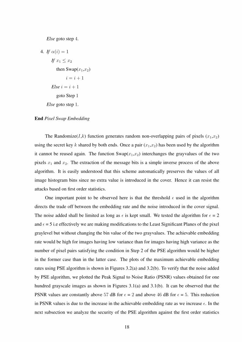
Figure 3.3: Result of testing PSE algorithm against Sample Pair Attack for ε = 5. Red Plot:Actual Message Length, Blue Plot: Predicted Message Length
h(I) = h(0), h(1), h(2), . . . , h(L−1). We then categorize the image pixels into two streams,
Embedding Stream and the Restoration Stream. During embedding we maintain the meta data
about those pixels which get changed during embedding and the amount of change in those
pixels. Then we compensate the histogram with the pixels from the Restoration Stream using
the meta data information such that the original histogram of the cover can be restored. So
by restoration we try to equalize h(I) and h(I). The algorithm is formalized in the next few
subsections.
3.3.1 Mathematical Formulation of Proposed Scheme
The proposed restoration scheme is dependent on the embedding scheme. The whole idea of
embedding and restoring is that some of image pixels are used for embedding and rest are
used for restoration. Without loss of generality, we can say that if number of pixels used for
embedding is greater than 50% of the whole image then complete restoration is not possible but
converse is not always true. One cannot say that if number of available compensation pixels are
greater than or equal to 50% of the whole image, then full compensation is possible. But we
can certainly see that the probability of full compensation increases with increase in the number
of pixels available for compensation. So a trade off has to be sought between the embedding
rate and restoration percentage in order to get the optimum embedding procedure. For better
understanding of the algorithm some definitions are described next.
22

Let the cover image, stego image (i.e. embedded but not yet compensated) and compen-
sated stego image (stego image after compensation) be defined byC, S andR respectively. Sup-
pose Cij , Sij and Rij represent the (i, j)th pixel of C, S and R images respectively (0 < i < m,
0 < j < n, m is number of rows and n is number of columns of image matrices).
Embed Matrix(Ψ): It is a m× n characteristic matrix representing whether a pixel has been
used for embedding or not.
Ψ(i, j) =
1 if (i, j)th pixel is used for embedding
0 if (i, j)th pixel is not used for embedding
(3.1)
Compensation V ector(Ω): It is a one dimensional vector with length L where L is number of
existing gray levels in the cover image (C). Ω(k) = u means that u number of pixels with gray
value k can be used for restoration.
Changed Matrix(Γ): It is a L × L matrix where L is number of existing gray levels in the
cover image (C). Γ(x, y) = λ means during embedding λ number of pixels are changed from
gray value x to gray value y.
Changed Matrix (Γ) is computed as given below:
Γ(x, y) =m∑i=0
n∑j=0
eq(Cij, x)× eq(Sij, y)× εij (3.2)
where
eq(a, b) =
1 if a = b
0 if a 6= b
(3.3)
Compensation Matrix(ξ): It is a L × L matrix where L is number of existing gray levels in
the cover image (C). ξ(x, y) = λ means during embedding number of times x is changed to y
minus number of times y changes to x is λ.
Compensation Matrix (ξ) has been formed as following:
ξ = UT (Γ− ΓT ) (3.4)
where UT (M) means upper triangulation of matrix M .
23

3.3.2 Algorithm Statistical Restoration
The statistical restoration algorithm is summarized below:
Algorithm: Statistical Restoration Algorithm (SRA)
Input: Cover Image (I)
Input Parameters: Compensation Matrix (ξ), Changed Matrix (Γ)
Output: Stego Image (Is)
Begin
for all k ∈ ξ(i, j) do
1. k = ξ(i, j)
2. If k > 0, k number of pixels with gray value i from the set of pixels used for compensa-
tion are changed to gray value j for full compensation.
Else k pixels with gray value j from the set of pixels used for compensation are changed
to gray value i for full compensation.
3. Modify the Compensation V ector (Ω) to reflect the pixel changes under taken in step 2
as in Equation 3.5 below
Ω(i) =
Ω(i)− k if Ω(i) > k
0 if Ω(i) ≤ k
(3.5)
End Statistical Restoration Algorithm (SRA)
In the above algorithm we have made the assumption that for Ω(i) < k, full compensation
is not possible. Further research can be possible to improve this situation.
24

3.3.3 Restoration with Minimum Distortion
The additional noise added due to compensation is an important issue. The goal is to design a
restoration procedure in such a way that additional noise should be kept minimum. In the SRA
algorithm, the noise introduced depends on the embedding algorithm used. The total noise (η)
introduced at the time of restoration can be estimated by
η =L−1∑i=0
abs[h(i)−h(i)]∑j=1
abs(i− kj) (3.6)
where h(i) and h(i) is the histogram of the stego and cover images respectively. L− 1 is
the no. of bins in the histogram. kj (0 ≤ kj ≤ L− 1) is a bin that is used to repair at least one
unit of data in ith bin.
Lemma 3.3.1 With any restoration scheme the minimum total noise∑L−1i=0 abs[h(i)− h(i)].
Proof: The total noise (η) introduced at the time of restoration is
η =L−1∑i=0
abs[h(i)−h(i)]∑j=1
abs(i− kj) (3.7)
where 1 ≤ abs(i − kj) ≤ L − 1. η is minimum when abs(i − kj) = 1. Substituting
abs(i− kj) = 1 in Equation 3.7 we get
η =L−1∑i=0
abs[h(i)− h(i)] (3.8)
Lemma 3.3.2 The total noise (η) added by the SRA algorithm is minimum if maximum noise
per pixel due to embedding is 1.
Proof: Since the SRA algorithm is based on pixel swapping strategy introduced in 3.2 i.e. if a
the gray level value α of a pixel is changed to β during steganographic embedding, at the time
of restoration, a pixel with gray level value β is changed to α.
During embedding with ±1 embedding, the gray level value of a pixel, x can be changed
into either x+ 1 or x− 1. Hence during restoration the proposed scheme restores bin x value is
repaired from either bin x+ 1 or x− 1 according to embedding. It is to be noted that maximum
noise that can be added during restoration for one member of a bin is at most 1 since we are
using only the neighboring bins for compensation. Hence, with ±1 embedding scheme (or any
25

other steganographic scheme where noise added during embedding per pixel is at most 1), the
proposed scheme increments or decrements gray value by 1 i.e. abs(i− ki) = 1.
From Equation 3.7, the total noise (η) introduced at the time of restoration is
η =∑L−1i=0
∑abs[h(i)−h(i)]j=1 abs(i− kj)
and for the SRA algorithm abs(i− ki) = 1, substituting this value in Equation 3.7, we get
η =∑L−1i=0
∑abs[h(i)−h(i)]j=1 (1)
or
η =∑L−1i=0 abs[h(i)− h(i)]
So from Lemma 1 and 2, we can conclude that the SRA algorithm adds minimum amount
of noise during restoration if maximum noise per pixel due to embedding is at most 1.
3.3.4 Experimental Results
For testing the performance of the SRA algorithm we conducted experiments on a data set of
one hundred grayscale images 3.4. Least Significant Bit replacement with embedding rate 0.125
bits/pixel is used as the embedding method. All of the images used in our experiment had non-
Gaussian histograms. Figures 3.5a, 3.6a and 3.7a image histograms of the three test images
(Dinosaur, Baboon, and Hills) respectively. Figures 3.5b, 3.6b and 3.7b show the difference
histograms of the two images before compensation. Figures 3.5c, 3.6c and 3.7c depict the
difference Histogram after compensation using Solanki. et als scheme and Figures 3.5d, 3.6d
and 3.7d show the compensation results using the proposed SRA algorithm respectively. It may
be seen that the proposed scheme provides better restoration than Solanki. et. al’s scheme.
Figure 3.8 shows the scatter plot of the reduction in the difference histogram for Solanki’s
scheme against proposed scheme. It can be observed that reduction in difference histogram is
more for the SRA algorithm.
3.3.5 Security Analysis
As already mentioned above many steganalysis techniques use first order statistical features to
detect stego images [34, 38, 39]. If the SRA algorithm is used then it may be possible to reduce
26
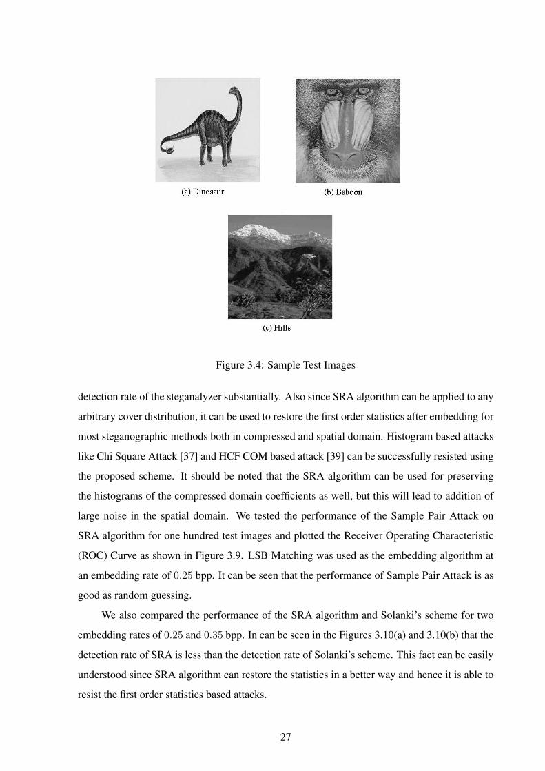
Figure 3.4: Sample Test Images
detection rate of the steganalyzer substantially. Also since SRA algorithm can be applied to any
arbitrary cover distribution, it can be used to restore the first order statistics after embedding for
most steganographic methods both in compressed and spatial domain. Histogram based attacks
like Chi Square Attack [37] and HCF COM based attack [39] can be successfully resisted using
the proposed scheme. It should be noted that the SRA algorithm can be used for preserving
the histograms of the compressed domain coefficients as well, but this will lead to addition of
large noise in the spatial domain. We tested the performance of the Sample Pair Attack on
SRA algorithm for one hundred test images and plotted the Receiver Operating Characteristic
(ROC) Curve as shown in Figure 3.9. LSB Matching was used as the embedding algorithm at
an embedding rate of 0.25 bpp. It can be seen that the performance of Sample Pair Attack is as
good as random guessing.
We also compared the performance of the SRA algorithm and Solanki’s scheme for two
embedding rates of 0.25 and 0.35 bpp. In can be seen in the Figures 3.10(a) and 3.10(b) that the
detection rate of SRA is less than the detection rate of Solanki’s scheme. This fact can be easily
understood since SRA algorithm can restore the statistics in a better way and hence it is able to
resist the first order statistics based attacks.
27

Figure 3.5: Results for Dinosaur
28

Figure 3.6: Results for Baboon
29

Figure 3.7: Results for Hills
30
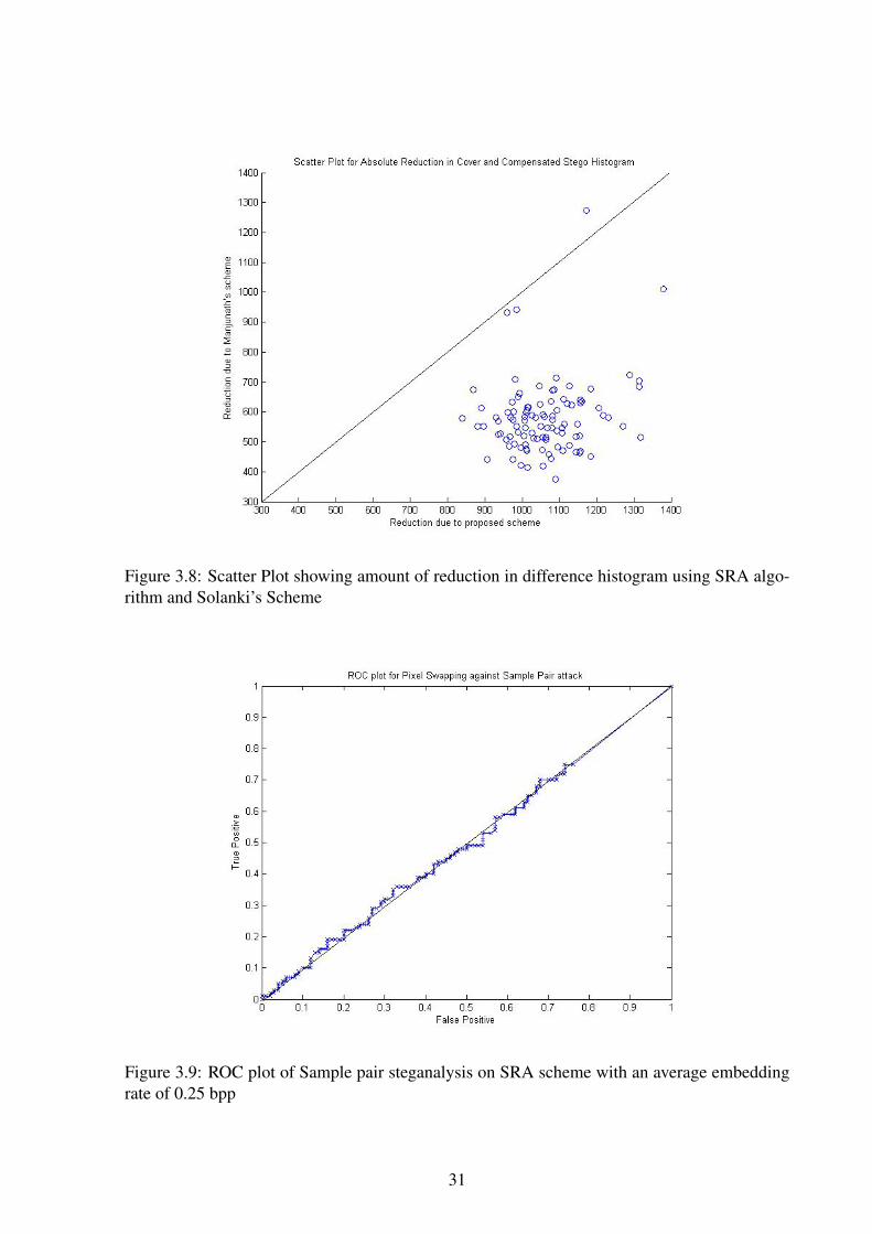
Figure 3.8: Scatter Plot showing amount of reduction in difference histogram using SRA algo-rithm and Solanki’s Scheme
Figure 3.9: ROC plot of Sample pair steganalysis on SRA scheme with an average embeddingrate of 0.25 bpp
31

(a) Embedding Rate = 0.25 bpp
(b) Embedding Rate = 0.35 bpp
Figure 3.10: Comparison of SRA algorithm and Solanki’s scheme against Sample Pair Attack.X-axis: Images, Y-axis: Predicted Message Length, Red Plot: Solanki’s Scheme, Blue Plot:SRA Algorithm
32
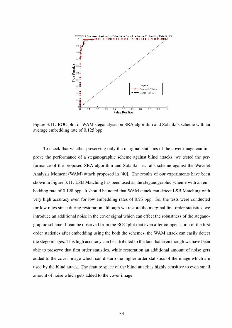
Figure 3.11: ROC plot of WAM steganalysis on SRA algorithm and Solanki’s scheme with anaverage embedding rate of 0.125 bpp
To check that whether preserving only the marginal statistics of the cover image can im-
prove the performance of a steganographic scheme against blind attacks, we tested the per-
formance of the proposed SRA algorithm and Solanki. et. al’s scheme against the Wavelet
Analysis Moment (WAM) attack proposed in [40]. The results of our experiments have been
shown in Figure 3.11. LSB Matching has been used as the steganographic scheme with an em-
bedding rate of 0.125 bpp. It should be noted that WAM attack can detect LSB Matching with
very high accuracy even for low embedding rates of 0.25 bpp. So, the tests were conducted
for low rates since during restoration although we restore the marginal first order statistics, we
introduce an additional noise in the cover signal which can effect the robustness of the stegano-
graphic scheme. It can be observed from the ROC plot that even after compensation of the first
order statistics after embedding using the both the schemes, the WAM attack can easily detect
the stego images. This high accuracy can be attributed to the fact that even though we have been
able to preserve that first order statistics, while restoration an additional amount of noise gets
added to the cover image which can disturb the higher order statistics of the image which are
used by the blind attack. The feature space of the blind attack is highly sensitive to even small
amount of noise which gets added to the cover image.
33

3.4 Summary
In this chapter two new algorithms have been proposed which are able to preserve the first or-
der statistics of a cover image after embedding and thus making the data hiding process robust
against first order statistic based steganalytic attacks. Moreover the proposed SRA algorithm
does not assume any particular distribution for the cover image and hence gives better perfor-
mance than existing restoration scheme given in [21, 22] especially for non-Gaussian covers. It
must be mentioned that the additional noise added during restoration is dependent on the em-
bedding algorithm for proposed scheme and is a topic of future research. It was also observed
that preservation of only the marginal statistics does not increase the robustness of a stegano-
graphic algorithm against blind steganalytic attacks as they are based on extremely high order
statistical moments which are sensitive to even small amounts of additive noise.
34

Chapter 4
Spatial Desynchronization
In this chapter a new steganographic framework is proposed which can prevent the calibration
based blind steganalytic attack in JPEG steganography. The calibration attack is one of the most
successful attacks to break the JPEG steganographic algorithms in recent past. The key feature
of the calibration attack is the prediction of cover image statistics from a stego image. To resist
the calibration attack it is necessary to prevent the attacker from successfully predicting the
cover image statistics. The proposed framework is based on reversible spatial desynchronization
of cover images which is used to disturb the prediction of the cover image statistics from the
stego image. A new steganographic algorithm based on the same framework has also been
proposed. Experimental results show that the proposed algorithm is less detectable against
the calibration based blind steganalytic attacks than the existing JPEG domain steganographic
schemes.
4.1 Introduction
Joint Photographics Expert Group (JPEG) image format is perhaps the most widely used format
in the world today and a lot of steganographic algorithms have been developed which exploit
the code structure of JPEG format. For example in JPEG steganography, Least Significant Bits
of non-zero quantized Discrete Cosine Transform (DCT) coefficients are used for embedding
[17, 18, 19]. However this causes significant changes in DCT coefficients and it is often used as
a feature for steganalysis. Westfeld’s F5 algorithm [17] tries to match the host statistics by either
increasing, decreasing, or keeping unchanged, the coefficient value based on the data bit to be
hidden. Provos’s OutGuess [18] was the first attempt at explicitly matching the DCT histogram
35
so that the first order statistics of the DCT coefficients can be maintained after embedding.
Sallee [19] proposed a model based approach for steganography where the DCT coefficients
were modified to hide data such that they follow an underlying model. Perturbed Quantization
proposed in [20] attempts to resemble the statistics of a double-compressed image. Statisti-
cal restoration method proposed by [21, 22] is able to perfectly restore the DCT coefficients
histogram of the cover after embedding, thus providing provable security so long as only the
marginal statistics are used by the steganalyst.
Significant research effort has also been devoted to developing steganalytic algorithms for
detecting the presence of secret information in an innocent looking cover image as already cov-
ered in section 2.2. The blind attacks, first proposed in [12] and [13] try to estimate a model
of an unmodified image based on some statistical features. One of the existing approaches for
predicting the cover image statistics from the stego image itself is by nullifying the changes
made by the embedding procedure to the cover signal. The most popular attacks based on this
approach was proposed by Pevny and Fridrich [14]. They estimated the cover image statistics
by a process termed as Self Calibration. The steganalysis algorithms based on this self cal-
ibration process can detect the presence of steganographic noise with almost 100% accuracy
even for very low embedding rates [14, 28].
In this chapter, we propose a new steganographic framework called Spatial Block Desyn-
chronization which attempts to resist the calibration based steganalytic attacks by preventing
the successful prediction of the cover image statistics from the stego image. We also intro-
duce a new steganographic scheme called Spatially Desynchronized Steganographic Algorithm
(SDSA) based on the same framework. We use a novel Statistical Hypothesis Testing Model
to show that the proposed SDSA scheme is more robust against calibration attack than Quanti-
zation Index Modulation (QIM)[23] and ”yet another steganographic scheme”(YASS)[15]. We
also evaluate the security of SDSA against several blind steganalysis attacks and compare the
performance of the algorithm against YASS[15], which is also found to be quite robust against
calibration based attacks [14, 28].
The rest of the chapter is organized as follows: In section 4.2 we discuss the calibration
based attacks and also present statistical tests to demonstrate its effectiveness. The possible
counter measures for resisting calibration attacks are discussed in section 4.3. The proposed
scheme is described in section 4.4, Experimental results are presented in section 4.5 finally the
chapter is concluded in section 4.6.
36

4.2 Calibration Attack
As already discussed in section 2.2.2, the process of self-calibration, tries to minimize the im-
pact of embedding in the stego image in order to estimate the cover image features from the
stego image. This calibration is done by decompressing the stego JPEG image to spatial do-
main and cropping 4 rows from the top and 4 columns from the left and recompressing the
cropped image. The next two subsections briefly explain the calibration attacks proposed in
[14] and [28] respectively.
4.2.1 23 Dimensional Calibration Attack
Let C and S be the cover and corresponding stego images and C and S be the respective
cropped images. The feature set for cover images (say F23C) and the stego images (say FS23)
are 23 dimensional vectors which are computed using the following equations
F(i)23C =
∥∥∥g(i)(C)− g(i)(C)∥∥∥L1
(4.1)
F(i)23S =
∥∥∥g(i)(S)− g(i)(S)∥∥∥L1
(4.2)
where L1 represents the L1 NORM of the two feature vectors, i = 1, 2, . . . 23 and g are
vector functionals which are applied to both cover and cropped cover and stego and cropped
stego images. These functionals are the global DCT coefficient histogram, co-occurrence ma-
trix, spatial blockiness measures etc. The complete set of functionals can be found in [14]. For
the rest of the chapter, we use the notation 23 DCA to refer to the 23 Dimensional Calibration
Attack.
4.2.2 274 Dimensional Calibration Attack
In the 274 dimensional calibration attack, 193 extended DCT features and 81 Markov features
are combined to form a 274 dimensional feature set which is then used to train the steganalytic
classifier. 193 DCT features have been derived by extending the features of 23 DCA [14] and
the 81 Markov features are derived from the 324 dimensional Markov features proposed in
[30] which models the difference between absolute value of neighboring DCT coefficients as a
Markov process. Let C and S be the cover and corresponding stego images and C and S be the
37
respective cropped images. The feature set for cover images (say F274C) and the stego images
(say F274S) are 274 dimensional vectors which are computed using the following equations
F274C(z) = γ(i)(j)(C)− γ(i)
(j)(C) (4.3)
F274S(z) = γ(i)(j)(S)− γ(i)
(j)(S) (4.4)
where z = 1, 2, . . . 274, γ(i) denote the vector functionals where i = 1, 2, . . . 21 and
j = 1, 2, . . . σi where∑21i=1 σ
i = 274. Each γ(i) yields σi features. These functionals are the
global DCT coefficient histogram, co-occurrence matrix, spatial blockiness measures etc. The
complete set of 21 functionals can be found in [28]. The most important difference between
23 dimensional attack and 274 dimensional attack is that in 274 dimensional attack absolute
differences between cover image and cropped cover image vectors (stego image and cropped
stego image vectors) are taken as cover (stego) features unlike the 23 dimensional attack where
L1 norm of the difference of the various functionals are taken as the feature set. For the rest of
the chapter, we use the notation 274 DCA to refer to the 274 Dimensional Calibration Attack.
4.2.3 Statistical Test for Calibration Attack
In this subsection, we propose a new Statistical Hypothesis Testing Framework to check the
following:
• Sensitivity of the features used in the calibration attacks.
• Effectiveness of the self-calibration process.
We extract the steganalytic features from the cover images and the corresponding stego
images using the calibration attacks as explained above. We then apply the Rank-Sum Test
[29] (also called the Wilcoxon-Mann-Whitney test) which is a non-parametric test for assessing
whether two samples of observations come from an identical population. The two hypothesis
are formulated as follows:
Null Hypothesis H0: The two samples have been drawn from identical populations
38
Alternate Hypothesis H1: The two samples have been drawn from different populations
The Rank-Sum test computes the U statistic for the two samples to accept or reject the
null hypothesis. The U statistic for the two samples are defined as follows:
U1 = W1 −n1 × (n1 + 1)
2(4.5)
U2 = W2 −n2 × (n2 + 1)
2(4.6)
where W1 and W2 are the sums of the ranks alloted to the elements of the two sorted
samples and n1, n2 are the sizes of the two samples. The detailed discussion on Rank-Sum test
can be found in [29].
We have used the Rank-Sum Test available in the Statistical Toolbox of MATLAB version
7.1 for our experiments. We measure the p-value from the Rank Sum Test where p is the
probability of observing the given result by chance if the null hypothesis is true. Small values
of p increase the chances of rejecting the null hypothesis whereas high values of p suggest
lack of evidence for rejecting the null hypothesis. QIM has been used as the steganographic
algorithm.
We first check the sensitivity of the features used by 23 DCA and 274 DCA. The 23
and 274 dimensional feature vectors are separately reduced to a single dimension using Fisher
Linear Discrimant(FLD) Analysis [31] for both the cover image features and the stego image
features. These single dimension values are labeled as the cover image sample and the stego
image sample for each of the attacks. We then test the hypothesis that the two samples are
drawn from an identical population or not. The test is applied on samples of size one thousand
each drawn from the cover image population and the stego image population respectively. The p
value observed from the test is recorded in Table 4.1 for both attacks at various embedding rates.
It can be observed that with the increase of embedding rate from 0.05 bpnc to 0.10 bpnc, the
p-value between the cover and the stego sample decreases to zero implying that the separation
between cover and stego population increases with increase of the embedding rate thus showing
that the features are indeed sensitive to the embedding.
In the second test, we test the effectiveness of the self-calibration process. This test has
only been applied to 274 DCA because for 23 DCA the final features are computed using
Equations 4.1 and 4.2 and it is not possible to calculate these features for a cover(stego) image
39

Table 4.1: p value of the Rank-Sum Test for 23 DCA and 274 DCA
Embedding p-value
Rate 23 DCA 274 DCA
0.05 2.1556× 10⁻⁸ 3.179× 10−87
0.10 0 0
0.25 0 0
0.50 0 0
and its cropped version individually. For the cover and the cropped cover images, we extract
the two 274 dimensional vectors αC and αC using the following equations:
αC(z) = γ(i)(j)(C) (4.7)
αC(z) = γ(i)(j)(C) (4.8)
where z = 1, 2, . . . 274. There are 21 vector functionals denoted as γ(1), γ(2), . . . γ(21) and
j = 1, 2, . . . σi where∑21i=1 σ
i = 274. Each γ(i) produces σi features as mentioned in subsection
4.2.2. αC and αC are 274 dimensional vectors.
Next we calculate the L2 NORM (LC2 ) between αC and αC using the following equation:
LC2 =
√√√√274∑i=1
[αC(i)− αC(i)]2 (4.9)
where αC and αC are 274 dimensional vectors.
We similarly calculate the L2 NORM (LS2 ) between αS (stego) and αS (cropped stego).
These two single dimensional values, LC2 and LS2 , are treated as two separate samples. We then
test the hypothesis that these two samples have been drawn from an identical population or
not. This hypothesis testing is done for different embedding rates of the QIM algorithm and the
p-value obtained from these tests are presented in Table 4.2. It can be observed that when the
embedding rate increases the p value decreases significantly. Thus we can conclude that the L2
NORM between stego and cropped stego increases with the increase of embedding rate. This
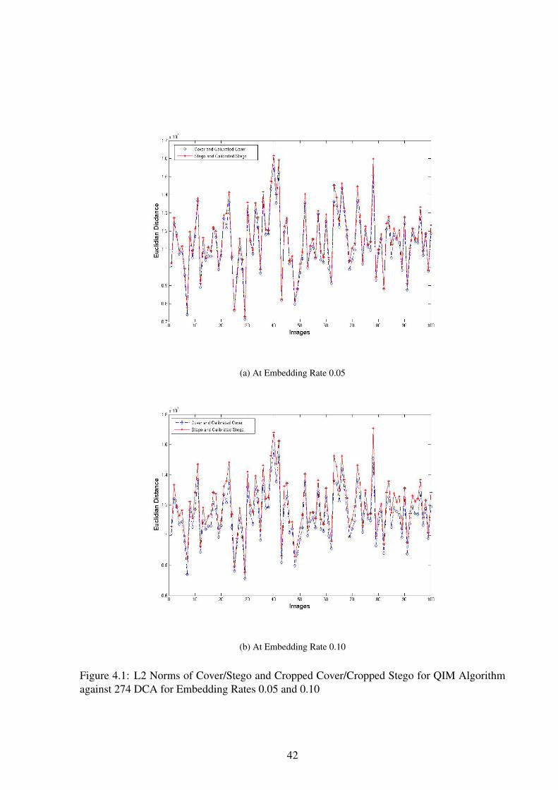
fact can also be observed in Figures 4.1 and 4.2. At embedding rate of 0.05 there is a very small
difference between the L2 NORM of Cover and Cropped Cover and the L2 NORM of Stego and
40

Table 4.2: p value of the Rank-Sum Test for 274 DCA for testing the Self Calibration Process
Embedding p value
Rate
0.05 0.1907
0.10 0.0059
0.25 1.028× 10⁻¹⁶
0.50 0
Cropped Stego (Figure 4.1(a)). With the increase of embedding rate (i.e., Emb. Rate = 0.10,
0.25 and 0.50), this difference also increases (Figure 4.1(b), 4.2(a) and 4.2(b)). Hence we can
conclude that statistics drawn from the cropped stego image can be used for approximating the
cover image statistics.
41
(a) At Embedding Rate 0.05
(b) At Embedding Rate 0.10
Figure 4.1: L2 Norms of Cover/Stego and Cropped Cover/Cropped Stego for QIM Algorithmagainst 274 DCA for Embedding Rates 0.05 and 0.10
42
4.3 Counter Measures to Blind Steganalysis
As mentioned above, the crux of blind steganalysis is its ability to predict the cover image
statistics using the stego image only. So a secure steganographic embedding might be possible if
the steganographer can somehow disturb the prediction step of the steganalyst. Some techniques
following the same line of thought have been proposed in steganographic literature. In [24], it
has been argued that estimation of cover image statistics can be disturbed by embedding data at
high embedding rates. By embedding data with high strength, the cover image is distorted so
much that the cover image statistics can no longer be derived reliably from the stego image. But
embedding at high rates will obviously increase the visual distortion introduced in the image.
Moreover as pointed out in [15], it might be possible to detect the embedding by testing a stego
image against an approximate model of a natural image.
In [15] the authors have suggested the use of randomized hiding to disable the estimation
of the cover image statistics. It has been observed that due to randomization of hiding, even
if the embedding algorithm is known to the steganalysts, they are unable to make any con-
crete assumptions about the hiding process. This approach has been extended to a successful
steganographic algorithm called ”yet another steganographic scheme” (YASS). It has been ex-
perimentally shown that the YASS algorithm can resist many blind attacks with almost 100%
success rate. But the main limitation of the YASS algorithm is that it is unable to achieve high
embedding rates.
In [26], the authors have suggested two modifications to the original YASS algorithm to
improve the achievable embedding rates. Firstly they randomize the choice of the quantization
matrix used during the embedding step. This choice of quantization matrix is made image
adaptive by using high quality quantization matrices for blocks having low variance and low
quality matrices for blocks having high variance values since a block having high variance by
itself supports high embedding rates as the number of non-zero AC coefficients increase in the
block.
The second modification is targeted towards reducing the loss in the message bits due
to the JPEG compression of the embedded image. The JPEG compression is considered as
an ”attack” which tries to destroy the embedded bits, thereby increasing the error rate at the
decoder side. Since the parameters of this attack i.e. the quality factor used for compression are
known after embedding, an iterative process of embedding and attacking is suggested so that
43

(a) At Embedding Rate 0.25
(b) At Embedding Rate 0.50
Figure 4.2: L2 Norms of Cover/Stego and Cropped Cover/Cropped Stego for QIM Algorithmagainst 274 DCA for Embedding Rates 0.25 and 0.50
44

the system converges towards a low error rate. The suggested modifications have been able to
improve the embedding rate upto some extent while maintaining the same levels of security. But
clearly the iterative step of embedding and attacking increases the complexity of the algorithm.
It will be shown in the next few sections that the proposed scheme can achieve even higher
embedding rates at same levels of security. In the next subsection we introduce our concept of
spatial block desynchronization for resisting the blind steganalytic attacks.
4.3.1 Spatial Block Desynchronization
In the JPEG image format, an image is divided into non-overlapping blocks of size 8× 8. The
information contained in these blocks is then compressed by taking the 2D Discrete Cosine
Transform of the block followed by quantization step which are then used for embedding data
bits. A slight alteration of this spatial block arrangement can desynchronize the whole image.
Such alteration of the spatial block arrangement of an image is termed as Spatial block desyn-
chronization. For example, 8 × 8 non overlapping blocks for embedding can be taken from a
subimage of the original cover image or we can say the block arrangement is slightly shifted
from standard JPEG compression block arrangement. A formal description of spatial block
desynchronization is given below.
Let I be a gray scale image of size (N×N ). A subimage of I can be obtained by removing
u rows from the top and v columns from left. Let us denote the cropped image by Iu,v. The size
of image Iu,v is (N − u)× (N − v). Let us denote the cropped portion of the image by Iδu,v i.e
I , Iu,v and Iδu,v are related by the following equation
Iδu,v = I − Iu,v (4.10)
So, the image I is partitioned into Iu,v and Iδu,v. The said partitioning is depicted pictorially
in Figure 4.3. In Figure 4.3, the partition Iu,v is denoted by portion labeled as EFGC and Iδu,v
by the portion labeled as ABEFGD.
An image I can be divided into a set of non overlapping block of size n × n (as shown
in Figure 4.3). Let this set be denoted by P (n×n)I and a block B is an element of set P (n×n)
I .
In Figure 4.3, these blocks are drawn with dashed lines. For JPEG compressed images n = 8
and the set of blocks is denoted by P (8×8)I . Now the cropped image Iu,v can be divided into a
set of non overlapping blocks of size m× n. Let this set be denoted by P (m×n)
Iu,v. In Figure 4.3,
45

Figure 4.3: Block Diagram of Spatial Block Desynchronization
P(m×n)
Iu,vset of blocks is drawn with solid lines. The spatial arrangement of P (m×n)
Iu,v(where the
actual embedding is done) is shifted from P(n×n)I . This spatial shifting of P (m×n)
Iu,vachieves the
required spatial desynchronization.
Another possible way of spatial desynchronization is to use a block size other than 8 × 8
i.e using blocks of sizes m × n where m 6= 8 and n 6= 8. In such a case, the quantization
matrix Q has to be changed accordingly to size m × n at the time of data embedding. This
deynchronization can be strengthened further with the help of randomization. In this case, the
removal of rows and columns and also the sizes of the blocks can be chosen randomly using a
shared secret key. Also, the matrix Q can be a shared secret between the two communicating
parties. Since at the steganalysis stage the image statistics are derived using blocks of sizes 8×8,
the steganalyst is not able to capture effectively the modifications made during the embedding
process. Even if it is known that embedding has been done using blocks of different sizes,
it is difficult to track the portions of the image containing the embedded information due to
randomized hiding.
It should be noted that once the quantized DCT coefficients have been obtained, any JPEG
steganographic scheme can be employed for embedding. In the next section we explain a new
steganographic scheme based on the concept of spatial block desynchronization.
46
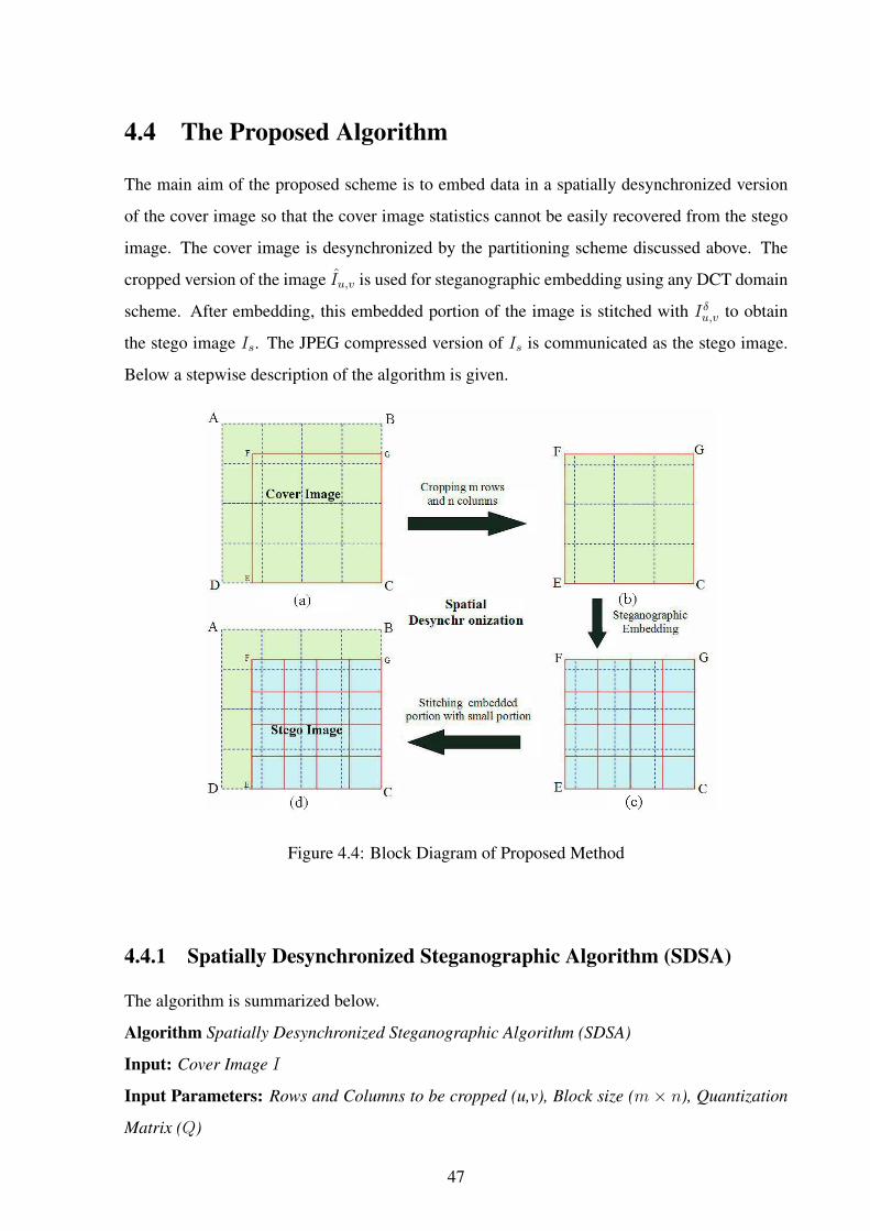
4.4 The Proposed Algorithm
The main aim of the proposed scheme is to embed data in a spatially desynchronized version
of the cover image so that the cover image statistics cannot be easily recovered from the stego
image. The cover image is desynchronized by the partitioning scheme discussed above. The
cropped version of the image Iu,v is used for steganographic embedding using any DCT domain
scheme. After embedding, this embedded portion of the image is stitched with Iδu,v to obtain
the stego image Is. The JPEG compressed version of Is is communicated as the stego image.
Below a stepwise description of the algorithm is given.
Figure 4.4: Block Diagram of Proposed Method
4.4.1 Spatially Desynchronized Steganographic Algorithm (SDSA)
The algorithm is summarized below.
Algorithm Spatially Desynchronized Steganographic Algorithm (SDSA)
Input: Cover Image I
Input Parameters: Rows and Columns to be cropped (u,v), Block size (m × n), Quantization
Matrix (Q)
47

Output: Stego Image Is
Begin
1. Partition the cover image I into Iu,v and Iδu,v by cropping u topmost rows and v leftmost
columns.
2. Performm×n non-overlapping block partitioning on Iu,v. Let us denote this set of blocks
by P (m×n)
Iu,v.
3. Choose a set of blocks from P(m×n)
Iu,v(using a key shared by both ends) and perform the
embedding in each of the selected blocks using any standard DCT based steganographic
scheme. The quantization matrix Q which is a shared secret is used for obtaining the
quantized coefficients.
4. Apply dequantization and Inverse Discrete Cosine Transform (IDCT) to the set of blocks
used for embedding in Step 3.
5. Join Iδu,v with the resulting image obtained at Step 4. This combined image is the output
stego image Is which is compressed using JPEG compression and communicated as the
stego image.
End Spatially Desynchronised Steganographic Algorithm (SDSA)
The SDSA algorithm has been shown pictorially in Figure 4.4. Figure 4.4(a) shows the
unmodified cover image from which the cropped image Iu,v (Figure 4.4(b)) is extracted. This
portion is labeled as EFGH in Figure 4.4(a). Iu,v is then divided into non overlapping blocks
size m × n as shown by solid lines in Figure 4.4(c). A DCT domain steganographic scheme
is then applied to some of these blocks and Iu,v is finally attached with Iδu,v to obtain the stego
image Is as shown in Figure 4.4(d).
23 DCA crops 4 rows and 4 columns from the top and the left of the image and uses the re-
maining portion of the image for estimating the cover image statistics. To disturb this calibration
step, at the time of embedding u rows and v columns (where u, v 6= 4 or any multiple of 8)
should be cropped from the left and the top of the image. Thus the cover image is spatially
desynchronized before actual embedding is done. During steganalysis, the steganalyst uses the
stego portion of the image itself as a reference for estimating the cover image statistics and
48

hence is not able to distinguish the cover image statistics from the stego image statistics. It
should be noted that if u consecutive rows and v consecutive columns are cropped from an im-
age, then u, v 6= 4 or any multiple of 8 because such kind of cropping will realign the blocks
of the partitioned image I2 with the original cover image and hence in effect there won’t be any
desynchronization during embedding.
Also since the embedded image undergoes JPEG compression before being communicated
to the decoding end, some of the embedded data bits might get lost in the process because of
the quantization step during JPEG compression. This quantization loss occurs for almost all
the DCT domain embedding schemes. We try to circumvent this problem by embedding data
mainly in the low-frequency DCT coefficients. Also embedded data can be made secure by
adding some redundant bits in the data stream and using error-control coding techniques. This
problem of using error-control coding for securing the data bits has been addressed in [23] albeit
at the cost of low embedding rate. We would like to mention here that in our implementations
of QIM, YASS and SDSA we have not included any error-control technique. Hence we shall be
comparing the raw versions of the three schemes. In the next section we verify our claim using
statistical hypothesis testing.
4.4.2 Hypothesis Testing
In this subsection, we use hypothesis testing to validate our claim that the SDSA algorithm does
disturb the self-calibration process of a steganalytic attack. We extract the steganalytic features
from the cover images and the corresponding stego images as explained in section 4.2.3. for
all the three schemes. Once again we observed the p values obtained from the Rank-Sum Test
which are presented in Tables 4.3 and 4.4. It can be seen that for all embedding rates the p-value
of the SDSA algorithm is greater than the p-value of both YASS and QIM scheme indicating
that the SDSA algorithm generates a stego image population which is statistically closer to
the cover image population than the populations generated by YASS and QIM. It should be
noted that even though the p-values obtained are small but for the purpose of comparison it is
significantly higher for the proposed scheme than that of QIM and YASS.
49
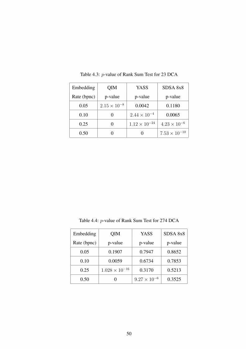
Table 4.3: p-value of Rank Sum Test for 23 DCA
Embedding QIM YASS SDSA 8x8
Rate (bpnc) p-value p-value p-value
0.05 2.15× 10⁻⁸ 0.0042 0.1180
0.10 0 2.44× 10⁻⁴ 0.0065
0.25 0 1.12× 10⁻²⁴ 4.23× 10⁻⁶
0.50 0 0 7.53× 10⁻¹⁰
Table 4.4: p-value of Rank Sum Test for 274 DCA
Embedding QIM YASS SDSA 8x8
Rate (bpnc) p-value p-value p-value
0.05 0.1907 0.7947 0.8652
0.10 0.0059 0.6734 0.7853
0.25 1.028× 10⁻¹⁶ 0.3170 0.5213
0.50 0 9.27× 10⁻⁶ 0.3525
50

4.5 Experiments and Results
For testing the performance of the SDSA algorithm we conducted experiments on a data set of
two thousand test images [16] which were divided into two equal sets of one thousand cover
images and one thousand stego images. Each image was resized to 256 × 256 with a JPEG
quality factor of 75%. For ease of comparison we have used QIM as the data embedding al-
gorithm and compare the performance of the SDSA algorithm with the original YASS[15] and
the QIM scheme itself. It has already been reported in [15] that YASS surpasses some of the
standard data hiding techniques like OutGuess[18] and StegHide[27]. So SDSA has not been
compared with OutGuess and StegHide. The embedding rate is expressed in terms of the non-
zero DCT coefficients available after quantization of the whole cover image i.e. in terms of
bits per non-zero coefficients (bpnc). We tested the performance of SDSA against 23 DCA and
Farid’s 92 Dimensional Attack proposed in [13]. Farid’s Attack is a DCT domain steganalysis
attack and it was used to test whether SDSA and spatial desynchronization can be used to defeat
steganalysis algorithms not based on self-calibration. The source code of the attack is available
at [32]. Area under the ROC and the Detection accuracy (Pdetect)[15] which is computed using
equations 4.11 and 4.12 have been used as the evaluation metrics.
Pdetect = 1− Perror (4.11)
Perror =1
2× PFP +
1
2× PFN (4.12)
where PFP , PFN are the probabilities of false positive and false negative respectively. A
value of Pdetect = 0.5 shows that the classification is as good as random guessing and Pdetect =
1.0 shows a classification with 100% accuracy.
Two possible cases of SDSA were tested during the experiments. In the first case after
cropping of rows and columns from the left and the top of the image, Iu,v is divided into blocks
of size 8× 8. In the second case, Iu,v is divided into blocks of sizes 10× 10. The quantization
matrix was adjusted accordingly by replacing the additional rows and columns by 50 which is
the quantization index for the highest frequency component at a JPEG quality factor of 75%.
We use the notation SDSA 8× 8 and SDSA 10× 10 respectively for the two cases of the SDSA
algorithm. 5 rows and 5 columns were cropped for both SDSA 8 × 8 and SDSA 10 × 10 i.e.
u = 5 and v = 5. YASS scheme was implemented using a big block size of 10 and a quality
51
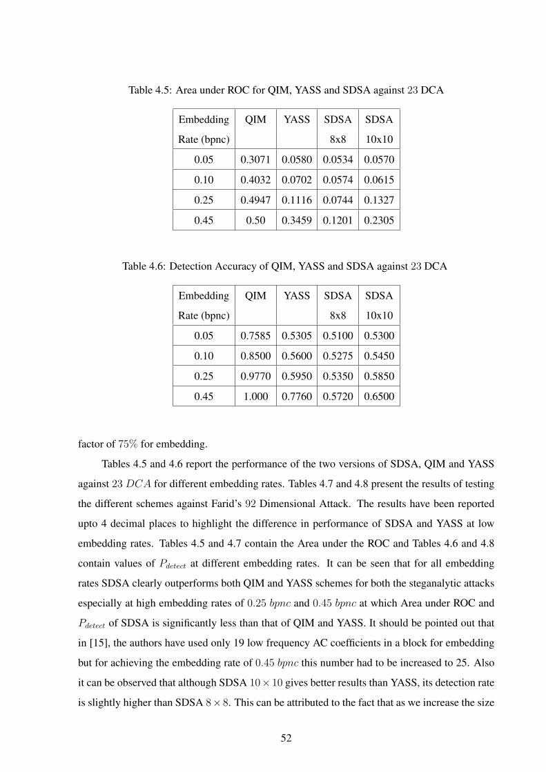
Table 4.5: Area under ROC for QIM, YASS and SDSA against 23 DCA
Embedding QIM YASS SDSA SDSA
Rate (bpnc) 8x8 10x10
0.05 0.3071 0.0580 0.0534 0.0570
0.10 0.4032 0.0702 0.0574 0.0615
0.25 0.4947 0.1116 0.0744 0.1327
0.45 0.50 0.3459 0.1201 0.2305
Table 4.6: Detection Accuracy of QIM, YASS and SDSA against 23 DCA
Embedding QIM YASS SDSA SDSA
Rate (bpnc) 8x8 10x10
0.05 0.7585 0.5305 0.5100 0.5300
0.10 0.8500 0.5600 0.5275 0.5450
0.25 0.9770 0.5950 0.5350 0.5850
0.45 1.000 0.7760 0.5720 0.6500
factor of 75% for embedding.
Tables 4.5 and 4.6 report the performance of the two versions of SDSA, QIM and YASS
against 23 DCA for different embedding rates. Tables 4.7 and 4.8 present the results of testing
the different schemes against Farid’s 92 Dimensional Attack. The results have been reported
upto 4 decimal places to highlight the difference in performance of SDSA and YASS at low
embedding rates. Tables 4.5 and 4.7 contain the Area under the ROC and Tables 4.6 and 4.8
contain values of Pdetect at different embedding rates. It can be seen that for all embedding
rates SDSA clearly outperforms both QIM and YASS schemes for both the steganalytic attacks
especially at high embedding rates of 0.25 bpnc and 0.45 bpnc at which Area under ROC and
Pdetect of SDSA is significantly less than that of QIM and YASS. It should be pointed out that
in [15], the authors have used only 19 low frequency AC coefficients in a block for embedding
but for achieving the embedding rate of 0.45 bpnc this number had to be increased to 25. Also
it can be observed that although SDSA 10×10 gives better results than YASS, its detection rate
is slightly higher than SDSA 8×8. This can be attributed to the fact that as we increase the size
52

Table 4.7: Area under ROC for QIM, YASS and SDSA against Farid’s 92 Dimensional Attack
Embedding QIM YASS SDSA SDSA
Rate (bpnc) 8x8 10x10
0.05 0.1082 0.0989 0.0844 0.0980
0.10 0.1125 0.1030 0.0853 0.1000
0.25 0.1987 0.1572 0.1044 0.1368
0.45 0.4960 0.2670 0.1360 0.2420
Table 4.8: Detection Accuracy of QIM, YASS and SDSA against Farid’s 92 Dimensional Attack
Embedding QIM YASS SDSA SDSA
Rate (bpnc) 8x8 10x10
0.05 0.5700 0.5140 0.5120 0.5090
0.10 0.6000 0.5210 0.5195 0.5100
0.25 0.6750 0.5900 0.5310 0.5870
0.45 0.9750 0.6750 0.5600 0.6650
of the embedding block the number of blocks available for embedding decrease and thereby
increasing the embedding density i.e. the bits/block and hence increasing the detection rate.
4.6 Summary
In this chapter, a new steganographic framework is proposed to resist calibration based blind
steganalytic attacks. The proposed framework which is based on spatial block desynchroniza-
tion to disturb the successful prediction of cover image statistics from the stego image which
is the key feature of calibration based steganalytic attacks. The proposed framework has been
extended to a new steganographic algorithm called “Spatially Desynchronized Steganographic
Algorithm (SDSA)”. A comparative study with existing steganographic schemes has been car-
ried out at different embedding rates on the basis of Area under the ROC and Detection Accu-
racy. It has been found that proposed algorithm shows better results than existing schemes in
terms of detectability against calibration based steganalytic attacks.
53
Chapter 5
Conclusions and Future Directions
5.1 Conclusions
In this thesis we have explored two different approaches to steganography. The first approach
was aimed at preservation of the marginal statistics of a cover image. The preservation of
marginal statistics helps in defeating the targeted attacks designed for specific steganographic
algorithms. We covered two kinds of algorithms under this approach. The first algorithm was
designed to inherently preserve the first order statistics of the cover image while embedding
itself. It has been shown that this approach is able to resist first order statistics based targeted
attacks while maintaining an acceptable quality of the stego image. The second algorithm
was an attempt at explicitly restoring the marginal statistics of the image after data has been
embedded in the image. It was found that under a specified constraint the suggested algorithm
is optimal in terms of the noise added due to the restoration procedure. It was also observed that
although the restoration of the image statistics can resist targeted attacks, it does not improve the
security of an embedding algorithm against blind attacks. This observation was attributed to the
fact that the restoration process acts as an additional source of noise in the cover signal which
can be captured during feature extraction and classification. This factor limits the applicability
of this approach to only targeted attacks.
The second approach studied in this thesis aims at hampering the steganalysts ability to
effectively estimating the statistics for classification. A new statistical model for testing the
efficiency of calibration based blind attacks was proposed. It was found that the calibration step
is indeed able to estimate an image model. To counter this, a generalized framework has been
proposed which disturbs this model estimation of the attack. It is based on embedding data such
54

that the stego population remains statistically closer to the cover population and the difference
between these two cannot be observed in the statistics drawn from the two populations. The
framework was extended to a new algorithm for JPEG domain steganography. This algorithm
was evaluated in the proposed statistical testing framework and it was found that the algorithm
is successful in breaking the calibration based blind attacks.
5.2 Future Directions
During the course of this work, some potential directions of future research were identified.
Firstly, it was observed that most of the steganographic research till date has been towards
designing algorithm which generate stego images which are as close to the cover as possi-
ble. All the algorithms study the behavior of the cover image while ignoring the message bit
stream. It may be possible to design some encoding functions, which given a cover image and
an embedding algorithm can modify the message stream such that it becomes more suitable for
embedding than the original bit stream. This kind of steganography can be useful even in the
“Active Warden Framework” of steganography because firstly the modified message stream will
be introducing less artifacts in the cover. Secondly, even if the embedding algorithm is known
to the attacker, the exact message sequence cannot be reconstructed unless the attacker has the
knowledge of the encoding function.
Another possible direction of research can be formulated as a problem of “Image Re-
trieval”. It is based on searching for a suitable cover image given a message sequence and the
embedding algorithm. This may be possible through maintaining a huge image database and
given any message sequence and a pseudo-random key for generating embedding locations,
we search for a cover image from the database that will generate a stego image with mini-
mum amount of changes. The change criterion considered for searching can be dependent on
the features used by the corresponding steganalytic attacks. Some other possible ideas can be
borrowed from the field of “Visual Cryptography” which encrypts a message by distributing
the decoding key into different images such that the message can be broken only by a proper
combination of these images.
55

Bibliography
[1] N. F. Johnson, and S. Jajodia, “Steganography: Seeing the Unseen”, IEEE Computer,
Feb. 1998,pp. 26-34.
[2] J. Mielikainen,“LSB Matching Revisited”, IEEE Signal Processing Letters , vol. 13, no.
5,May 2006, pp. 285 - 287 .
[3] A. Ker,“Steganalysis of Embedding in Two Least-Significant Bits”, IEEE Trans. on Infor-
mation Forensics and Security, vol. 2, no. 1, March 2007, pp. 46-54.
[4] X. Zhang , and S. Wang, “Steganography using multiple-base notational system and hu-
man vision sensitivity, IEEE Signal Processing Letters, vol. 12, Issue 1, Jan. 2005, pp.
67-70.
[5] D.C. Wu, and W.H. Tsai, “A Steganographic method for images by pixel-value differenc-
ing”, Pattern Recognition Letters, vol. 24, Jan. 2003, pp. 1613–1626.
[6] H.C. Wu, N.I. Wu, C.S. Tsai, and M.S. Hwang, “Image steganographic scheme based
on pixel-value differencing and LSB replacement methods”, IEE Proc. Vision, Image and
Signal Processing, vol. 152, Oct. 2005, pp. 611-615.
[7] R. Crandall, “Some Notes on Steganography”, Posted on Steganography Mailing List,
1998.
[8] A. Sur, P. Goel, and J. Mukhopadhyay, “A Spatial Domain Steganographic Scheme for
Reducing Embedding Noise”, in Proc. 3rd International Symposium on Communications,
Control and Signal Processing (ISCCSP 2008), St. Julians, Malta, 12-14 March, pp. 1024
- 1028.
56

[9] A. Sur, P. Goel, and J. Mukhopadhyay, “A SDS based Steganographic scheme for reducing
Embedding Noise”, 15th International Conference on Advanced Computing and Commu-
nication, (ADCOM-2007), Guwahati, India, 18-21 Dec., pp. 771-775.
[10] I.J. Cox, J. Kilian, F.T. Leighton, T. Shamoon, “A Secure, Robust Watermark for Multi-
media”, in Proc. of the 1st Int. Workshop on Information Hiding, Cambridge, U.K, 30th
May - 1 June 1996 ,pp. 185-206.
[11] E. Koch, and J. Zhao, “Towards Robust and Hidden Image Copyright Labeling”, in Proc.
IEEE Workshop on Nonlinear Signal and Image Processing, Halkidiki, Greece, June.
1995, pp. 452-455.
[12] I. Avcibas, N. Memon, and B. Sankur, “Steganalysis using Image Quality Metrics”, IEEE
Trans. on Image Processing, vol. 12, Feb 2003, pp. 221-229.
[13] H. Farid, and L. Siwei, “Detecting Hidden Messages Using Higher-Order Statistics and
Support Vector Machines”, in Proc. 5th Int. Workshop on Information Hiding, Noordwijk-
erhout, The Netherlands, 7-9 Oct. 2002, pp. 340-354.
[14] J. Fridrich, “Feature-Based Steganalysis for JPEG Images and its Implications for Future
Design of Steganographic Schemes”, in Proc. 6th Int. Workshop on Information Hiding,
Toronto, Canada, 23-25 May 2004, pp. 67-81.
[15] K. Solanki, A. Sarkar, and B.S. Manjunath, “YASS: Yet Another Steganographic Scheme
that Resists Blind Steganalysis”, in Proc. 9th Int. Workshop on Information Hiding, Saint
Malo, Brittany, France,11-13 June 2007, pp. 16-31.
[16] J. Wang , J. Li, and G. Wiederhold, “SIMPLicity : Semantics-sensitive integrated match-
ing for picture LIbraries”, IEEE Trans. on Pattern Analysis and Machine Intelligence, vol.
23, no. 9, Sept. 2001, pp. 947-963.
[17] A. Westfeld, “High capacity despite better steganalysis (F5 - a steganographic algorithm)”,
in Proc. 4th Int. Workshop on Information Hiding, Pittsburgh, PA, USA, pp. 289-302, 25-
27 April 2001.
[18] N. Provos, “Defending against statistical steganalysis”, in Proc. 10th USENIX Security
Symposium, vol. 10, pp. 24-24, Washington DC, 2001.
57

[19] P. Sallee, “Model-based steganography”, in Proc. 2nd International Workshop on Digital
Watermarking, Seoul, Korea, pp. 154-167, 20-20 Oct. 2003.
[20] J. Fridrich, M. Goljan, P. Lisonek, and D. Soukal, “Writing on wet paper”, IEEE Trans.
on Signal Processing, Special Issue on Media Security, vol. 53, Oct. 2005, pp. 3923-3935.
[21] K. Solanki , K. Sullivan, U. Madhow, and B.S. Manjunath, and S. Chandrasekaran, “Sta-
tistical restoration for robust and secure steganography”, in Proc. IEEE Int. Conf. on Image
Processing, Genova, Italy, vol. 2, 11-14 Sep. 2005, pp. 1118-1121.
[22] K. Solanki , K. Sullivan, U. Madhow, B.S. Manjunath, and S. Chandrasekaran, “Probably
secure steganography: Achieving zero K-L divergence using statistical restoration”, in
Proc. IEEE Int. Conf. on Image Processing, Atlanta, GA, USA, 8-11 Oct. 2006, pp. 125-
128.
[23] K. Solanki, N. Jacobsen, U. Madhow, B.S. Manjunath, and S. Chandrasekaran, “Robust
image-adaptive data hiding based on erasure and error correction”, IEEE Trans. on Image
Processing, vol. 13, no. 12, Dec. 2004, pp. 1627-1639.
[24] M. Kharrazi, H.T. Sencar, and N. Memon, “Cover selection for steganographic embed-
ding”, in Proc. Int. Conf. Image Processing. Atlanta, GA, USA, pp. 117-120, 8-11 Oct.,
2006.
[25] X.G. Xia, C.G. Boncelet, and G.R. Arce, “A multiresolution watermark for digital im-
ages”, IEEE Int. Conf. on Image Processing, Washington, DC, USA, 26-29 Oct. 1997.
[26] A. Sarkar, K. Solanki, and B.S. Manjunath, “Further Study on YASS: Steganography
Based on Randomized Embedding to Resist Blind Steganalysis”, in Proc. SPIE - Secu-
rity, Steganography, and Watermarking of Multimedia Contents X, San Jose, California,
vol. 6819, pp. 681917-681917-11 , Jan. 2008.
[27] S. Hetzl, and P. Mutzel, “A graph theoretic approach to steganography”, in Proc. 9th IFIP
Int. Conf. on Communications and Multimedia Security, Salzburg, Austria, pp. 119-128,
19-21 Sep. 2005.
[28] T. Pevny , and J. Fridrich, “Merging Markov and DCT features for multi-class JPEG ste-
ganalysis”, in Proc. SPIE, Electronic Imaging, Security, Steganography, and Watermark-
ing of Multimedia Contents IX, San Jose, CA, vol. 6505 , Jan 2007, pp. 03-04.
58

[29] R.A. Johnson, “Miller & Freund’s Probability and Statistics for Engineers”, Prentice Hall
of India Pvt. Ltd., New Delhi, 2003.
[30] C. Chen, Y.Q. Shi, W. Chen, and G. Xuan, “Statistical moments based universal steganal-
ysis using JPEG-2D array and 2-D characteristic function”, in Proc. Int. Conf. on Image
Processing, Atlanta, GA, USA, 8-11 Oct., 2006, pp. 105-108.
[31] R.O. Duda, P.E. Hart, and D.G. Stork, “Pattern Classification”, John Wiley & Sons Inc.,
New York, 2000.
[32] H. Farid, “http://www.cs.dartmouth.edu/farid/research/steg.m” (Code for generating
wavelet-based feature vectors for steganalysis.)
[33] J. Fridrich, and D. Soukal, “Matrix Embedding for Large Payloads”, IEEE Trans. on In-
formation Forensics and Security, vol. 1, Sept. 2006, pp. 390-395.
[34] S. Dumitrescu, X. Wu, and N. Memon, “On steganalysis of random lsb embedding in
continuous-tone images”,in Proc. IEEE International Conference on Image Processing,
Rochester, New York., September 2002.
[35] J. Fridrich, T. Pevny, and J. Kodovsky, “Statistically Undetectable JPEG Steganography:
Dead Ends, Challenges, and Opportunities”, in Proc. ACM Multimedia and Security Work-
shop, Dallas, TX, 20-21 Sept. 2007, pp. 3-14.
[36] R Tzschoppe, R. Buml and J J. Eggers, “Histogram Modifications with Minimum MSE
Distortion”, Technical Report, December 18, 2001, Erlangen, Germany.
[37] R Chandramouli , M Kharrazi and N Memon, “Image Steganography and Steganalysis:
Concepts and Practices”, in Proc. 2nd Int. Workshop on Digital Watermarking, Seoul,
Korea, 20-22 Oct. 2003, pp. 35-49.
[38] J. Fridrich, M. Goljan and R. Dui, “Reliable Detection of LSB steganography in Color and
Grayscale Images”,in Proc. ACM Workshop on Multimedia and Security, Ottawa, CA, 5th
Oct. 2001, pp. 27-30.
[39] A.D. Ker, “Steganalysis of LSB matching in grayscale images”, IEEE Signal Processing
Letters, vol. 12,pp. 441–444, June 2005.
59
[40] J. Fridrich, M. Goljan, and T. Holotyak, “New Blind Steganalysis and its Implications”, in
Proc. SPIE Security, Steganography, and Watermarking of Multimedia Contents VIII, vol.
6072, pp. 607201, Jan. 2006
[41] J. J. Eggers, R. Bauml, and B. Girod, “A communications approach to image steganogra-
phy”, in Proc. SPIE Security and Watermarking of Multimedia Contents IV, vol. 4675, pp.
26-37, April 2002.
[42] J. Fridrich, M. Goljan, and D. Hogea,“Steganalysis of JPEG Images: Breaking the F5 Al-
gorithm”, in Proc. 5th International Workshop on Information Hiding, Noordwijkerhout,
The Netherlands, 79 Oct. 2002, pp. 310 - 323.
[43] J. Harmsen, and W. Pearlman, “Steganalysis of additive noise modelable information hid-
ing”, in Proc. Security and Watermarking of Multimedia Contents V, vol. 5020, June 2003,
pp. 131-142.
60
Top Related