


Languages
Pages
Legal


Daniel Salvador Vélez Parra
Análise analítica e numérica do rebaixamento temporario do lençol
freático em aquíferos granulares
Dissertação de Mestrado
Dissertação apresentada como requisito parcial para obtenção do titulo de Mestre pelo Programa de Pós-Graduação em Engenharia Urbana e Ambiental do Departamento de Engenharia Civil da PUC-Rio.
Orientador: Celso Romanel.
Rio de Janeiro Outubro de 2014

Daniel Salvador Vélez Parra
Análise analítica e numérica do rebaixamento temporario do lençol
freático em aquíferos granulares
Dissertação apresentada como requisito parcial para obtenção do titulo de Mestre pelo Programa de Pós-Graduação em Engenharia Urbana e Ambiental do Departamento de Engenharia Civil da PUC-Rio Aprovada pela Comissão Examinadora abaixo assinada.
Prof. Celso Romanel Presidente/Orientador
Departamento de Engenharia Civil – PUC-Rio
Profa. Ana Cristina Sieira
Departamento de Engenharia Civil – EURJ
Roberto Quevedo TecGraf - PUC-Rio
Prof. José Eugênio Leal
Coordenador Setorial de Pós-Graduação do Centro Técnico Científico - PUC-Rio
Rio de Janeiro, 16 de Outubro de 2014

Todos os direitos reservados. É proibida a
reprodução total ou parcial do trabalho sem
autorização da universidade, do autor e do
orientador.
Daniel Salvador Vélez Parra
Graduou-se em Engenharia Civil pela
Universidade de Cuenca (Cuenca-Equador) em
2009. Principais áreas de interesse: geotecnia
ambiental, hidrologia de aguas subterrâneas.
Ficha Catalográfica
CDD: 624
Vélez Parra, Daniel Salvador Análise analítica e numérica do rebaixamento temporário do lençol freático em aquíferos granulares / Daniel Salvador Vélez Parra; orientador: Celso Romanel. – 2014. 132 f. : il. (color.) ; 30 cm Dissertação (mestrado)–Pontifícia Universidade Católica do Rio de Janeiro, Departamento de Engenharia Civil, Programa de Pós-Graduação em Engenharia Urbana e Ambiental, 2014. Inclui bibliografia 1. Engenharia civil – Teses. 2. Rebaixamento. 3. Modelagem 3D. 4. Aquífero. 5. Elementos finitos. l. Romanel, Celso. II. Pontifícia Universidade Católica do Rio de Janeiro. Departamento de Engenharia Civil. III. Título.

Dedico este trabalho a Deus, e aos
meus queridos pais Remígio e Dora e
minha irmã Mary.

Agradecimentos
Ao meu orientador Professor Celso Romanel pela ajuda, amizade, apoio e todos
os conhecimentos transmitidos.
Aos meus pais, pela educação, e apoio incondicional e a minha irmã Mary pelo
seu carinho.
Aos professores que participaram da banca examinadora pelos valiosos
comentários que enriqueceram, o presente trabalho.
Aos meus amigos Christian Mejía, Raúl ``chato´´ Contreras, Grimaldo Romero,
Juliana``satanás´´ Carvalho e Tania Bustamante pela amizade e apoio.
A Paola Garcia pelo carinho e compressão.
Aos amigos da PUC-Rio pela amizade.
A todos meus familiares que sempre me deram seu apoio.

Resumo
Vélez Parra, Daniel Salvador; Romanel, Celso (Orientador). Análise
analítica e numérica do rebaixamento temporário do lençol freático em
aquíferos granulares. Rio de Janeiro, 2014. 132p. Dissertação de Mestrado
– Departamento de Engenharia Civil, Pontifícia Universidade Católica do
Rio de Janeiro.
O estudo do fluxo permanente de água em meios porosos, governado pela
equação diferencial de Laplace, é de grande importância em vários problemas da
engenharia civil e ambiental, como no comportamento de barragens, poços,
estabilidade de taludes, rebaixamento temporário do lençol freático, etc.
Dependendo das condições de contorno e das propriedades de permeabilidade dos
materiais envolvidos, uma solução aproximada deve ser buscada através de
métodos numéricos, como o método dos elementos finitos, implementado em
vários programas comerciais de computador atualmente. Um dos principais
aspectos a ser considerado é a influência do fluxo tridimensional nas soluções
que, na maioria das vezes, ainda é representado através de um problema de fluxo
2D, em virtude de vários fatores como a maior disponibilidade de programas
bidimensionais, da maior dificuldade na geração de malha de elementos finitos
3D, além do maior tempo de processamento e quantidade de memória necessários.
Esta dissertação aborda problemas de fluxo, nas condições 2D e 3D, envolvendo o
rebaixamento temporário do lençol freático em maciços de solos saturados. Os
exemplos analisados investigam um rebaixamento ocorrido na cidade de São
Paulo, para a construção de um shopping center e da construção da pequena
central hidrelétrica (PCH) Garganta da Jararaca no estado do Mato Grosso.
Comparações dos resultados numéricos são feitas com valores obtidos por
formulações analíticas e entre simulações realizadas com modelos bi e
tridimensionais. Nos estudos numéricos o rebaixamento foi implementado
prescrevendo-se as vazões nos poços bem como foi utilizada uma técnica
alternativa combinando infiltração e bombeamento no mesmo poço.
Palavras-chave
Rebaixamento; modelagem 3D; aquífero; elementos finitos.

Extended Abstract
Vélez Parra, Daniel Salvador; Romanel, Celso (Advisor). Analytical and
numerical analysis of temporary drawdown of phreatic level in
granular aquifers. Rio de Janeiro, 2014. 132p. MSc. Dissertation –
Departamento de Engenharia Civil, Pontifícia Universidade Católica do Rio
de Janeiro.
1 Introduction
The study of steady-state flow of groundwater is governed by the Laplace
equation and has great importance in several problems in civil and environmental
engineering related to earth dams, wells, slope stability, etc. Depending on
boundary conditions and properties of soil an approximate solution is normally
obtained by numerical methods, such as the finite difference method or the
popular finite element method, implemented in several commercial computer
programs available nowadays.
One of the main aspects that must be considered is the influence on the
solution of the tridimensional flow since in most computational studies the
problem is represented by a 2D mesh, partly due to the greater availability of bi-
dimensional programs, partly due the more complicated process of generating 3D
finite element meshes and the required computer resources in terms of RAM
memory and CPU times.
In this thesis the main characteristics of groundwater flow are investigated
with 2D and 3D numerical models involving temporary dewatering of saturated
unconfined and confined aquifers. The engineering cases relate to the construction
of a shopping mall in the city of São Paulo (Brazil) and the construction of a small
hydroelectric power plant in the state of Mato Grosso (Brazil).
Comparisons of the results are made between numerical analyses and the
analytical formulation available for some ideal situations. The numerical solutions
were obtained either using the conventional scheme of prescribing a well
discharge or an alternative technique which combines infiltration and water
extraction in the same well.

2 Numerical model
In the first part of this study two cases of temporary drawdown reported by
Jin et al. (2011) and Powrie & Preene (1997) were replicated with the aim to
compare the feasibility of our model with respect to results already published in
the literature.
A technique called Nozzle-Suction-Infiltration described by Jin et al. (2011)
involves the simultaneous pumping and infiltration of water in unconfined
aquifers using the same well, with water extraction in the upper portion and
infiltration in the bottom of the aquifer. As mentioned by Jin (2011) in the
proximity of the injection point the pore pressure rises to create a hydraulic
barrier, cutting off the flow between the two portions of the well (extraction and
infiltration). In this research a 3D model with dimensions 60m x 60m in the
horizontal plane and 20m height was used. A single totally penetrating well in the
center of the finite mesh was created and subdivided into two parts, considering
water extraction in the upper part and water infiltration through the lower one.
The granular soil was a well-graded sand with hydraulic conductivity k = 1 x 10⁻³
m/s and porosity n = 0.25. Figure 1 presents the results obtained from the finite
element model considering a parametric variation of the following terms: a)
extraction/infiltration rate; b) infiltration depth; c) hydraulic conductivity; d) soil
anisotropy (kz ≠ kr).
a)
-1,00
-0,80
-0,60
-0,40
-0,20
0,00
0 5 10 15 20 25 30 35
Dra
wd
ow
n (
m)
Radial distance from the well (m)
Conventional dewatering: Qpumping=20m3/s
Qpumping=Qinfiltration=20m3/h
Qpumping=Qinfiltration=30m3/h
Qpumping=Qiinfiltration=40m3/h

b)
c)
d)
Figure 1 – Extraction/infiltration model considering a parametric variation: a) extraction/infiltration
rate; b) infiltration depth; c) hydraulic conductivity; d) soil anisotropy.
-1,00
-0,80
-0,60
-0,40
-0,20
0,00
0 5 10 15 20 25 30 35
Dra
wd
ow
n (
m)
Radial distance from the well (m)
Conventional dewatering
Infiltration depth 20m
Infiltration depth 17m
Infiltration depth 14m
Infiltration depth 11m
Infiltration depth 8m
-1,20
-1,00
-0,80
-0,60
-0,40
-0,20
0,00
0 5 10 15 20 25 30 35
Dra
wd
ow
n (
m)
Radial distance from the well (m)
k = 0,001 m/s
k = 0,002 m/s
k = 0,005 m/s
k = 0,0005 m/s
-1,20
-1,00
-0,80
-0,60
-0,40
-0,20
0,00
0 5 10 15 20 25 30 35
Dra
wd
ow
n (
m)
Radial distance from the well (m)
kz/kr = 0,1
kz/kr = 0,3
kz/kr = 0,5
kz/kr = 1

The second example deals with a comparative study between analytical
solutions and numerical results in a confined aquifer. The rectangular (a x b)
excavation in the middle of the 3D finite element mesh (Figure 2) had its length a
increased at every finite element analysis in order to get different values for the
normalized distance to the recharge source (Lo/a). The saturated hydraulic
conductivity was k = 5 x 10⁻⁵
m/s and the hydraulic head (H = 32m) was kept
constant in all lateral boundaries. The flow rate extracted with the dewatering
system installed along the excavation perimeter was also evaluated considering
analytical equations for the following situations: a) 2D plane flow; b) 2D radial
flow; c) combined plane and radial flow.
Figure 2 – 3D finite element mesh with a totally penetrating rectangular (a x b) excavation.
2.1. Plane flow
For a rectangular dewatering system with geometric (a >b) and close to a
recharge source, the flow could be considered essentially plane with a small part
due to the radial flow that occurs near the edges of the excavation. In this case the
flow rate can be estimated by the following equation:
𝑄 = 2𝑘𝐷(𝐻 − ℎ𝑤) [𝑎
𝐿𝑜+
𝜋
ln(2𝐿𝑜𝑏)] (2.1)
where D refers to the aquifer thickness, (H-hw) represents the drawdown, L0 the
distance from the recharge source and k the soil hydraulic conductivity.
Low permeability layer k =1x10⁻⁹
cm/s Initial water level H = 38 m

If the excavation length a is much greater than its width b (a>>b) the flow could
be admitted as plane only and equation 2.1 can be rewritten as:
𝑄 = 2𝑘𝐷(𝐻 − ℎ𝑤) (𝑎
𝐿𝑜) (2.2)
The analyses were carried out for excavations geometries a/b = 10, 20, and
50, keeping constant the distance to the recharge source (L0 = 50m) and the
prescribed hydraulic drawdown (H - hw = 5m). The flow rate obtained by the
finite element model (Qef) was compared with those calculated using the
analytical formulation (Q). Results are presented in Figure 3.
Figure 3 – Flow rate variation with normalized recharge distance (L0/a) obtained with the 3D finite
element model and analytical equations.
As can be seen in Figure 3, the consideration of an additional flow rate
generated from the edges of the excavation tends to overestimate the flow with
respect to the finite element results, mainly for values of the recharge source
distance Lo/a > 0,1. When applying the hypothesis of plane flow only (Eq. 2.2) the
analytical formulation overestimates the flow rate moderately, ranging from
approximately 20% for Lo/a = 0,01 to 50% for Lo/a = 0,1 and then remaining
constant up to Lo/a = 1. It may be concluded that as far the recharge source is
located, the greater the influence of the excavation geometry (a/b) on the plane
flow conditions.
0
0,5
1
1,5
2
2,5
3
0,01 0,10 1,00
Q/Q
ef
Lo/a
Contribuição dos extremos (a/b=10)Contribuição dos extremos (a/b=20)Contribuição dos extremos (a/b=50)Fluxo plano (a/b=10)Fluxo plano (a/b=20)Fluxo plano (a/b=50)
Radial and plane flow (a/b=10) Radial and plane flow (a/b=20) Radial and plane flow (a/b=50) Plane flow only (a/b=10) Plane flow only (a/b=20) Plane flow only (a/b=50)

2.2. Radial flow
For an excavation with similar dimensions (a ≈ b) and a recharge source
relatively distant, the flow turns essentially radial and the problem could be
analyzed as a circular well with an equivalent radius. In this case the flow rate can
be calculated by Eq. 2.3 (Thiem, 1906).
𝑄 =2𝜋𝑘𝐷(𝐻−ℎ𝑤)
𝑙𝑛(𝐿𝑜𝑟𝑒)
(2.3)
In this analysis the drawdown value (H - hw = 5m) was kept constant,
considering three excavation geometries (a/b = 1, 2, 5) while varying the distance
to the recharge source a ≤ L0 ≤ 20a. The equivalent well radius (re) was
determined in two ways: assuming an equivalent circular excavation area or an
equivalent circular excavation perimeter. Figure 4 presents a comparison of the
flow rates calculated with analytical formulation (Q) and the finite element
method (Qef). The numerical results were determined by 2D (Powrie e Preene,
1997) and 3D (this research) finite element analyses.
It was observed that the analytical solution approaches the numerical results
(2D and 3d cases) for values of recharge source distances between 7a < Lo < 10a.
The flow rate is underestimated for Lo > 10a and overestimated for Lo < 7a. The
way the equivalent well radius was determined shows irrelevant effects on the
results and a minor influence of excavation geometry a/b was detected for values
Lo < 5a, i.e. only when the recharge contour Lo is close enough of the excavation.
a)
0
0,5
1
1,5
2
2,5
3
1 10 100
Q/Q
ef
Lo/a
MEF 3D a/b=1.0
MEF 3D a/b=2.0
MEF 3D a/b=5.0
MEF 2D (Powrie e Preene, 1997) a/b=1.0
MEF 2D (Powrie e Preene, 1997) a/b=2.0
MEF 2D (Powrie e Preene, 1997) a/b=5.0

b)
Figure 4 – Comparison of flow determined from numerical and analytical analyses considering an
equivalent well radius as: a) re = √𝑎𝑏/𝜋; b) re = (𝑎 + 𝑏)/𝜋.
2.2. Radial and plane flow
For a rectangular excavation next to the recharge source, the flow is plane
with a radial flow contribution at the corners. In this situation, Cedergren (1989)
suggested the following modifications in equations Eqs. 2.1 and 2.2,
𝑄 = 2𝑘𝐷(𝐻 − ℎ𝑤) [𝑎+𝑏
𝐿𝑜+ 𝜋] (2.4)
𝑄 = 2𝑘𝐷(𝐻 − ℎ𝑤) [𝑎+𝑏
𝐿𝑜] (2.5)
Figure 5 presents the results (analytical flow rate Q, calculated with
equations 2.4 and 2.5, normalized with respect to the numerical flow rate Qef) for
rectangular excavations of geometries a/b = 1, 2, 5 situated from a recharge
source at distances between 0,1a < L0 < 10a. The following conclusions can be
drawn:
a) For L0/a < 0,2 there are significant differences between analytical and
numerical results, since the flow occurs in the condition of plane flow
essentially;
b) As the distance L0/a becomes larger, the flow calculated from equation 2.5
results smaller, indicating that the flow is turning gradually to radial;
0
0,5
1
1,5
2
2,5
3
3,5
1 10 100
Q/Q
ef
Lo/a
MEF 3D a/b=1.0
MEF 3D a/b=2.0
MEF 3D a/b=5.0
MEF 2D (Powrie e Preene, 1997) a/b=1.0
MEF 2D (Powrie e Preene, 1997) a/b=2.0
MEF 2D (Powrie e Preene, 1997) a/b=5.0

c) The excavation geometry (a/b) has a greater influence on results obtained
with the plane flow hypothesis than with the combined plane and radial
assumption.
d) The application of either Eqs. 2.4 or 2.5 overestimates the flow rate Q
when L0/a < 1;
e) When L0/a >1 the radial and plane flow hypothesis gives errors greater
than 150%.
Figure 5 – Comparative flow rates calculated by analytical equations and 3D finite elements
analyses.
3 Engineering cases
3.1. Brooklin Shopping Mall
The Brooklin Shopping Mall is located in the California Street, in the city of
Sao Paulo (Brazil). It was built in an area of 736 m2
equivalent to a rectangle of
46m length and 16m width. The field tests indicated the existence of two soil
layers: the upper one composed by soft clayey sand, from the natural ground level
to 3m deep, followed by a grey silty sand up to the depth of 19m (borehole limits).
The phreatic level was found 3 m from the natural ground level. Building
construction requirements specified drawdown of the phreatic level to a depth of
6,5m or, in other words, required an effective drawdown of 3,5m from the original
water level. The pumping system was based on 62 wellpoints, spaced 2m each,
with a total flow rate Q = 0,0156 m³/s measured in the field.
0
1
2
3
4
5
6
7
0,1 1 10
Q/Q
ef
Lo/a
Fluxo plano e radial nos extremos a/b=1.0Fluxo plano e radial nos extremos a/b=2.0Fluxo plano e radial nos extremos a/b=5.0Fluxo unicamente plano a/b=1.0Fluxo unicamente plano a/b=2.0Fluxo unicamente plano a/b=5.0
Plane and radial flow a/b=1.0 Plane and radial flow a/b=2.0 Plane and radial flow a/b=5.0 Plane flow only a/b=1.0 Plane flow only a/b=2.0 Plane flow only a/b=5.0

3.1.1. Analytical solution
The first analysis was made in terms of analytical formulation, using Eq.
3.1, and considered a circular well with equivalent excavation area. The recharge
source was assumed as radial, using Eq. 3.2 to determine its distance from the
center of the well.
𝑄 =𝜋𝑘(𝐻2−ℎ𝑤
2 )
𝑙𝑛(𝑅𝑜𝑟𝑒)
(3.1)
𝑅𝑜 = 3000(𝐻 − ℎ𝑤)√𝑘 (3.2)
where H = 16m is the initial hydraulic head in the unconfined aquifer, k = 3x10⁻⁵
m/s the isotropic hydraulic conductivity and s = H - hw = 1,2m the drawdown
calculated with Eq. 3.1.
Another analytical possibility when considering a rectangular excavation
(a/b > 1,5) in unconfined aquifers is to add the radial flow near the edges to the
plane flow in the middle region, as given by Eq. 3.3.
𝑄 =𝜋𝑘(𝐻2−ℎ𝑤
2 )
𝑙𝑛(𝑅𝑜𝑟𝑒)
+ 2 [𝑥𝑘(𝐻2−ℎ𝑤
2 )
2𝐿0] (3.3)
where x is the excavation length (x = 46 m) and Ro determined from Eq. 3.2. As
mentioned by Powers (2007) a linear recharge source will produce the same
recharge effect such as a radial source situated at twice the distance, i.e. Ro = 2Lo.
With this considerations the calculated drawdown was s = 1,5m.
3.1.2. 2D numerical solution
The problem was analyzed using the finite element program Plaxis 2D
v.2013 under the assumption of plane and axisymmetric flow. For the plane flow
model, the first soil layer of clayey sand was not considered because the
groundwater level passes through its base. The saturated hydraulic conductivity of
the aquifer is k = 3x10⁻⁵
m/s (Velloso, 1977; Huertas 2006) and the analysis

considered two orthogonal cross sections as shown in Figure 6. The computed
drawdown from the finite element analysis was s = 3m.
a)
b)
c)
d)
Figure 6 – 2D finite element analyses: a) cross section along the excavation length; b) cross section
along the excavation width; c) drawdown across the middle of the excavation length; d) drawdown
across the middle of the excavation width.
16 m
a = 46 m
16 m
b = 16 m
Ro = 58 m
Ro = 58 m
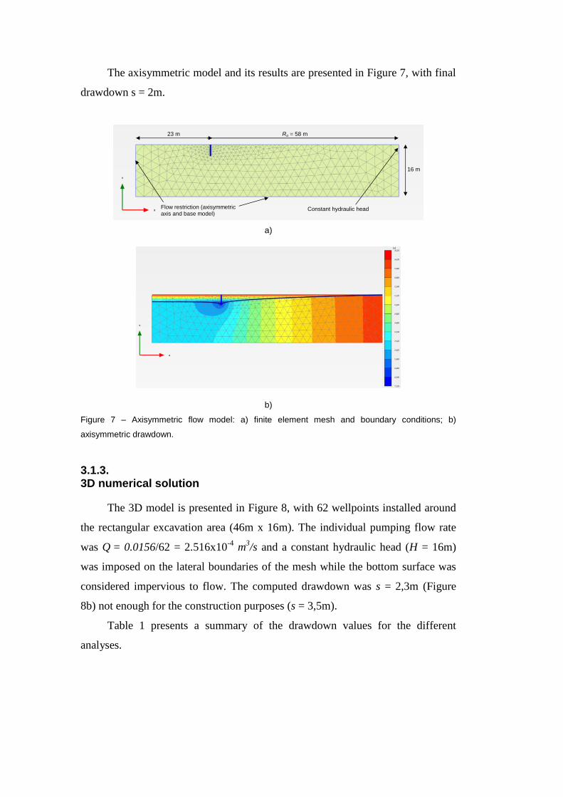
The axisymmetric model and its results are presented in Figure 7, with final
drawdown s = 2m.
a)
b)
Figure 7 – Axisymmetric flow model: a) finite element mesh and boundary conditions; b)
axisymmetric drawdown.
3.1.3. 3D numerical solution
The 3D model is presented in Figure 8, with 62 wellpoints installed around
the rectangular excavation area (46m x 16m). The individual pumping flow rate
was Q = 0.0156/62 = 2.516x10⁻⁴
m3/s and a constant hydraulic head (H = 16m)
was imposed on the lateral boundaries of the mesh while the bottom surface was
considered impervious to flow. The computed drawdown was s = 2,3m (Figure
8b) not enough for the construction purposes (s = 3,5m).
Table 1 presents a summary of the drawdown values for the different
analyses.
Ro = 58 m 23 m
16 m
Flow restriction (axisymmetric axis and base model)
Constant hydraulic head

Table 1 – Summary of the drawdown values
Type of analysis Flow rate Drawdown
(m3/s) (m)
Field measurements 0,0156 3,5
Equivalent well radius 0,0156 1,2
Equivalent well radius including radial flow near the excavation edges
0,0156 1,5
2D finite element model – plane flow 0,0156 3,0
2D finite element model – axisymmetric flow 0,0156 2,0
3D finite element model 0,0156 2,3
a)
b)
Figure 8 – 3D finite element analysis: a) mesh and boundary conditions; b) drawdown in the middle
of excavation.
3.1.4. Comments
The numerical plane flow model yielded a drawdown close to the measured
value in field, but this kind of analysis does not include the possibility of flow
perpendicular to the considered cross section. Similarly, an axisymmetric model
Constant hydraulic head Impervious base
Excavation area and pumping system

cannot provide accurate results since the excavation dimensions (a, b) are quite
different from each other to be accurately represented as a circular well.
However, the 3D finite element model provided a lower drawdown than the
actual field measurements, which could be possibly attributed to an inadequate
value of the hydraulic conductivity for the saturated aquifer.
3.2. Small hydroelectric plant Garganta da Jararaca
The small hydroelectric plant Garganta da Jararaca is located in the Sangue
River in the state of Mato Grosso (Brazil). For the construction of the power
house an area of 5072 m2 was excavated, equivalent to a rectangle (60m x 85m)
with its smallest side only 6m distant from the river. The excavation reached the
depth of 36m below the natural ground level.
From geotechnical tests (SPT and water infiltration tests) the soil profile
was characterized by a 6m thick residual soil layer followed by fine sandstone
between elevations 390m to 347m (borehole limit). The aquifer (second soil layer)
is unconfined with phreatic surface in El. 385m and average hydraulic
conductivity k = 2.4x10⁻⁵
m/s. Between El. 368m – 365m it was found a very
weathered sandstone layer.
For the power house construction it was necessary to lower the groundwater
to El. 360m in the middle of the excavation, approximately 25m below the
original water level. For this purpose a pumping system composed of 84 deep
penetrating wells (up to El. 345m) was installed along the perimeter of the
excavation, as shown in Figure 9. Since the field tests did not detect an
impervious base within the borehole limits, it was assumed in the next analytical
and numerical calculations that the aquifer extended to El. 275m (110m thick).
3.2.1. Analytical solution
The analysis was developed with the concept of equivalent radius well
considering the Sangue River (El. 378m) as a linear recharge source at only 6m
distance from the excavation border. Using the following equation the drawdown
was calculated in the middle of the excavation:

𝑄 =𝜋𝑘(𝐻2−ℎ𝑤
2 )
𝑙𝑛(2𝐿0𝑟𝑒
) (3.4)
where Q is the maximum flow rate measured in field (Q = 1399 m3/h) and k =
2.4x10⁻⁵
m/s is hydraulic conductivity. The drawdown was determined as s =
23,6m, a value close to the field measurement (s = 25m).
3.2.2. 2D numerical solution – axisymmetric flow
In the axisymmetric finite element model the Sangue river was assumed as
the recharge source for the homogeneous and isotropic aquifer with hydraulic
conductivity k = 2,4x10⁻⁵
m/s. The flow rate distributed along the excavation
perimeter was considered as q = 0,39/2π = 0.062 m3/s/rad. Figure 10 presents the
model mesh, boundary conditions and drawdown results with s = 25m in the
middle of excavation.
Figure 9 – The drawdown system at Garganta da Jararaca power plant.
Figure 10 – Axisymmetric model for the Garganta da Jararaca power plant (left) and drawdown
results (right).
re = 40,2 m 6 m
Flow restrictions
110 m
Constant hydraulic head (Sangue River)
Drawdown in the middle of excavation

3.2.3. 3D numerical solution
The finite element mesh may be seen in Figure 11a, with all the 84 wells
represented to the same depth reached in the field (36m from the natural ground
level) and spaced at every 3m. The total flow rate (Q = 0,39 m3/s) was divided
equally for each well (q = 16.65 m3/h). Field tests indicated that the water level
has a moderate inclination toward the Sangue river and for this reason the
hydraulic heads prescribed on the boundaries are different to each other: at El.
378m on the boundary correspondent to the river bank and at El. 385m for the
opposite boundary situated 410m away (Figure 11b). The maximum drawdown
computed with the 3D finite element model was s = 16m (Figure 12).
Table 2 presents all drawdown values determined with the analytical
formulation and finite element analyses (2D and 3D models).
a)
b)
Figure 11 – 3D model of Garganta da Jararaca power plant: a) finite element mesh; b) groundwater
configuration before drawdown.
Constant hydraulic head
Flow restriction
Excavation area
Pumping system
Initial phreatic level inclined toward riverside
Pumping system
Flow restriction (model base)

Figure 12 – Groundwater after dewatering: a) horizontal cross section close to the excavation
bottom; b) vertical cross section in the middle of excavation.
Table 2 – Drawdown values in the middle of the excavation for Garganta da Jararaca power plant.
Type of analysis Drawdown (m)
Field measurements 27
Finite Elements Method 3D 16
Finite Elements Method 2D (axisymmetric analysis) 25
Analytical formulation 23,6
3.2.4. Comments
The numerical analysis in the axisymmetric condition reached the best
approximation with respect to field measurements, in agreement with previous
results obtained by Corrêa (2006).
However, the results from numerical 3D analysis were quite different and
this discrepancy could be attributed to several uncertainties such as the pumping
flow rate at each well and the hydraulic conductivity of the aquifer. In comparison
with the 2D model, the flow incoming perpendicular to the plane of analysis
generates higher values of flow rate and, consequently, lower values of
drawdown. The purpose of the 3D simulation was also to verify the influence of
this component of flow in addition to the effects of the excavation geometry (a ≠
b), the different distances to the recharge boundaries and the slope of the original
groundwater level.
Keywords
Drawdown; 3D modeling; aquifer; finite elements.

Sumário
1. Introdução 34
2. Determinação de parâmetros hidráulicos em aquíferos 37
2.1. Meio poroso saturado e parcialmente saturado 37
2.2. Equação governante do fluxo permanente em meio
poroso saturado 38
2.3. Aquíferos granulares 42
2.4. Coeficiente de permeabilidade (k) 43
2.5. Ensaio de bombeamento em poços 46
2.5.1. Características do ensaio 46
2.5.2. Interpretação do ensaio em aquífero confinado 50
2.5.2.1. Método de Theis (1935) 50
2.5.2.2. Método de Cooper e Jacob (1946) 53
2.5.2.3. Método das distâncias de rebaixamento 56
2.5.2.4. Método de Thiem (1906) 56
2.5.3. Interpretação do ensaio em aquífero não confinado 58
2.5.3.1. Método de Theis modificado (1935) 58
2.5.3.2. Interpretação com curvas características 58
2.5.3.3. Método de Thiem (1906) 61
3. Rebaixamento temporário do lençol freático 64
3.1. Bombeamento direto 64
3.2. Ponteiras filtrantes 66
3.3. Sistema de injetores 69
3.4. Sistema de poços profundos 72
3.5. Dimensionamento analítico de um sistema de rebaixamento 73
3.5.1. Método do poço e da cava equivalentes 74
3.5.2. Fluxo radial para poço em aquífero confinado 76
3.5.3. Fluxo radial para poço em aquífero não confinado 76
3.5.4. Fluxo radial para poço em aquífero misto 77
3.5.5. Fluxo de uma fonte linear para cava equivalente 77

3.5.6. Resumo da formulação analítica 78
4. Modelagens numéricas de aferição 83
4.1. Rebaixamento do lençol freático com a técnica DSI 83
4.1.1. Modelo tridimensional de elementos finitos 84
4.1.2. Análise dos resultados 88
4.2. Comparação com soluções analíticas de poço e
cava equivalentes 89
4.2.1. Aquífero confinado com fluxo predominantemente plano 90
4.2.2. Aquífero confinado com fluxo predominantemente radial 93
4.2.3. Aquífero confinado com fluxo plano e radial 95
5. Estudo de casos 98
5.1. Shopping Brooklin 98
5.1.1. Descrição da obra 98
5.1.2. Solução analítica com poço equivalente 98
5.1.3. Solução numérica aproximada 2D 100
5.1.4. Solução numérica aproximada 3D 103
5.2. PCH Garganta da Jararaca 107
5.2.1. Descrição da obra 107
5.2.2. Perfis geotécnicos 107
5.2.3. Sistema de rebaixamento 110
5.2.4. Solução analítica aproximada 110
5.2.5. Solução numérica – fluxo axissimétrico 111
5.2.6. Solução numérica 3D com elementos de poço 112
5.2.7. Solução numérica 3D com elementos de vala drenante 118
5.2.8. Retroanálise do coeficiente de permeabilidade saturado 120
5.2.9. Solução numérica 3D com fluxo transiente 122
6. Conclusões e sugestões 126
7. Referências bibliográficas 129

Lista de Figuras
Figura 2.1 – Distribuição de poropressões em um maciço de
solo 37
Figura 2.2 – Fluxo através de um elemento infinitesimal no
meio poroso 38
Figura 2.3 – Condutividades hidráulicas em solo estratificado 39
Figura 2.4 – Variação da viscosidade da água µw (milipoises)
com a temperatura (ºC) (Cedergreen, 1967) 45
Figura 2.5 – Ensaio de dois aquíferos diferentes utilizando
um único poço: a) ensaio no aquífero inferior.
b) ensaio no aquífero superior. (adaptado de Powers 2007) 47
Figura 2.6 – Distribuição de piezômetros de monitoramento
no ensaio de bombeamento. a) aquífero em condições
normais. b) aquífero com contornos de recarga e impermeável.
(Adaptado de Powers, 2007) 48
Figura 2.7 – Curva de rebaixamento - logaritmo de tempo
para aquífero em condição ideal, aquífero com fonte de recarga,
aquífero com contorno impermeável (adaptado de Powers 2007) 49
Figura 2.8 – Ensaio com poço de bombeamento em aquífero
confinado. (Adaptado de Cedergreen, 1967) 51
Figura 2.9 – Método gráfico de Theis (Todd e Mays, 2005) 54
Figura 2.10 – Método gráfico de Cooper e Jacob, com tempo t
em minutos e rebaixamento s em metros (Todd e Mays, 2005). 55
Figura 2.11 – Método das distâncias de rebaixamento
(Watson e Burnett, 1995). 57
Figura 2.12 – Fluxo normal à área lateral de um cilindro. 39
Figura 2.13 – Interpretação com curvas características para
aquífero não confinado, considerando drenagem retardada
(Neuman, 1975). 59
Figura 2.14 – Ensaio com poço de bombeamento em
aquífero não confinado (Cedergreen, 1967). 62

Figura 3.1 – Rebaixamento do nível freático com bombeamento
aberto (Mansur e Kaufman, 1962). 64
Figura 3.2 – Sistema de ponteiras de múltiplo estágio
(Adaptado de Mansur e Kaufman, 1962) 66
Figura 3.3 – Espaçamento recomendável entre ponteiras:
a) areia e pedregulho uniforme e limpo, b) areia e
pedregulho estratificado. (Mansur e Kaufman, 1962). 67
Figura 3.4 – Profundidade recomendável em ponteiras para
algumas condições de campo: a) solo granular uniforme;
b) camada de argila próxima do fundo da escavação,
c) camada de solo grosso subjacente ao fundo da escavação.
(Adaptado de Powers, 2007). 68
Figura 3.5 – Ponteiras com válvulas de calibração
(adaptado de Powers, 2007). 69
Figura 3.6 – Princípio de funcionamento do bico Venturini
(Alonso, 1999) 70
Figura 3.7 – Sistema de rebaixamento com injetores de tubos
paralelos (Alonso, 1999). 71
Figura 3.8 – Sistema de rebaixamento composto de poço
profundo e ponteira filtrante (Mansur e Kaufman, 1962). 73
Figura 3.9 – Arranjo básico de poço profundo com bomba
submersa. (Adaptado de Powers, 2007). 73
Figura 3.10 – Poço equivalente, a) sistema circular, b) sistema
retangular (Powers, 2007). 74
Figura 3.11 – Fluxo radial para poço com redução da pressão
Do aquífero (adaptado de Powers, 2007). 77
Figura 3.12 – Fator B para poços parcialmente penetrantes
aquífero confinado (Mansur e Kaufman, 1962). 80
Figura 3.13 – Fator B para poços parcialmente penetrantes em
aquífero não confinado (Mansur e Kaufman, 1962). 81
Figura 3.14 – Fator λ para cavas parcialmente penetrantes em
aquífero confinado, (Mansur e Kaufman, 1962) 81
Figura 3.15 – Análise aproximada de um sistema de poços
com fluxo radial e linear combinados (adaptado de Powers,
2007). 82
Figura 4.1 – Poço no sistema DSI com regiões de extração e
reinjeção de água (Holzbecher et al. 2011) 84
Figura 4.2 – Malha de elementos finitos, poço de bombeamento
e pontos de controle dos resultados de carga hidráulica. 85
Figura 4.3 – Evolução do rebaixamento com variação de: a) vazão
de extração e infiltração; b) profundidade de infiltração;
c) condutividade hidráulica saturada k; d) anisotropia do solo (kv≠kh) 87
Figura 4.4 – Resultados DSI obtidos por Jin (2014) com variação
de k e anisotropia do solo 87
Figura 4.5 – Malha genérica de elementos finitos para análises
3D do rebaixamento do lençol freático. 89
Figura 4.6 – Modelo 3D nível freático inicial 90
Figura 4.7 – Configurações dos regimes de fluxo: a) fluxo
predominantemente plano; b) fluxo radial com fonte de recarga
distante; c) combinação de fluxo plano e radial (Powrie e
Preene, 1997). 90
Figura 4.8 – Variação da vazão calculada utilizando
formulação analítica (Q) e o método dos elementos finitos
3D (Qef) com a distância relativa (Lo/a) da fonte de recarga
para valores a/b = 10, 20 e 50. 92
Figura 4.9 – Fluxo 3D em aquífero confinado, relação a/b = 20 e
fonte de recarga próxima (Lo = 50m): a) a = 75m, b = 3.75m;
b) a = 200m, b = 10m; c) a = 1900m, b = 95m; d) a = 3000m,
b = 150m. 93
Figura 4.10 – Comparação das vazões para uma escavação
retangular com fonte de recarga L0 distante, utilizando
elementos finitos (2D e 3D) e formulação analítica do poço de
raio equivalente re: a) calculado com base na área equivalente
; b) calculado com base no perímetro equivalente. 94
Figura 4.11 – Comparação entre valores de vazão calculados por
formulação analítica e método dos elementos finitos em análises 3D 96

Figura 4.12 – Fluxo em escavação retangular com geometria
a/b = 2 e distância variável à fonte de recarga em
aquífero confinado: a) Lo = 10m; b) Lo = 50m; c) Lo = 80m;
d) Lo = 700m. 97
Figura 5.1 – Malha de elementos finitos: a) ao longo do
comprimento do terreno; b) ao longo da largura do terreno. 101
Figura 5.2 – Posição final do nível do lençol freático: a) ao longo
Do comprimento do terreno; b) ao longo da largura do terreno. 102
Figura 5.3 – Malha de elementos finitos análise axissimétrico 102
Figura 5.4 – Posição final do nível do lençol freático modelo
axissimétrico. 103
Figura 5.5 – Modelo 3D para análise do rebaixamento do lençol
Freático no Shopping Brooklin SP: a) malha de elementos finitos;
b) distribuição de cargas hidráulicas antes do rebaixamento. 104
Figura 5.6 – Distribuição das cargas hidráulicas na área da
escavação no plano horizontal situado na profundidade z = 3m 104
Figura 5.7 – Distribuição das cargas hidráulicas na seção vertical
central paralela ao comprimento do terreno. 105
Figura 5.8 – Distribuição das cargas hidráulicas na seção vertical
central paralela à largura do terreno. 105
Figura 5.9 – Coeficiente de permeabilidade para areia
siltosa saturada, segundo o conteúdo de silte e índice de 105
vazios (Bandini, 2009).
Figura 5.10 – PCH Garganta da Jararaca (Corrêa, 2006). 107
Figura 5.11 – Sondagens geotécnicas para construção da casa de
força (Corrêa, 2006). 108
Figura 5.12 – Perfil geotécnico na seção AA com localização
das sondagens e linha de escavação (Corrêa, 2006). 109
Figura 5.13 – Perfil geotécnico na seção BB com localização
das sondagens e linha de escavação (Corrêa, 2006). 109
Figura 5.14 – Planta do sistema de rebaixamento do nível do
lençol freático (Corrêa, 2006). 110
Figura 5.15 – Malha de elementos finitos (esquerda) e posição do

lençol freático após bombeamento (direita). 112
Figura 5.16 – Malha de elementos finitos para análise de
fluxo permanente 3D. 113
Figura 5.17 – a) Geometria da escavação e distribuição dos
poços de bombeamento; b) superfície freática com declividade em
direção à margem do rio. 114
Figura 5.18 – Distribuição de cargas hidráulicas no modelo antes
do rebaixamento. 114
Figura 5.19 – a) distribuição de cargas hidráulicas no
aquífero não confinado após o rebaixamento; b) posição
final da superfície freática; c) distribuição das cargas hidráulicas
em seção transversal horizontal próxima à base da escavação. 116
Figura 5.20 – Posição da linha freática (a); e linhas
equipotenciais (b) no plano central paralelo ao comprimento
da escavação (plano paralelo a XZ). 117
Figura 5.21 – Posição da linha freática (a); e linhas
equipotenciais (b) no plano central paralelo à largura da
escavação (plano paralelo a YZ). 118
Figura 5.22 – Modelo 3D com simulação de valas drenantes no
fundo da escavação. 119
Figura 5.23 – Rebaixamento do lençol freático e linhas
equipotenciais nos planos centrais: a) paralelo ao 120
comprimento da escavação (plano XZ), b) paralelo à
largura da escavação (plano YZ).
Figura 5.24 – Posição final da superfície freática na análise
numérica 2D (axissimetria). 121
Figura 5.25 – Distribuição das cargas hidráulicas após o
rebaixamento na análise numérica 3D. 121
Figura 5.26 – Posição final da superfície freática e linhas
equipotenciais na análise numérica 3D. 122
Figura 5.27 – Posição da linha freática ao longo do plano central
paralelo ao comprimento da escavação (paralelo ao plano XZ). 122
Figura 5.28 – Pontos de controle da variação de poropressão

na análise transiente. 123
Figura 5.29 – Variação da poropressão com o tempo nos pontos
de controle. 123
Figura 5.30 – Evolução no tempo das cargas hidráulicas no plano
central até atingir a condição de fluxo permanente. 125

Lista de Tabelas
Tabela 2.1 – Valores típicos de condutividade hidráulica em
solos naturais (Powers, 2007) 46
Tabela 2.2 – Valores da função de poço W(u) para vários
valores de u (Wenzel, 1942) 53
Tabela 3.1 – Condições desfavoráveis para bombeamento
direto (Powers, 1992)
65
Tabela 3.2 – Raio de influência (R0) segundo o tipo de solo
(Jumikis, 1962).
75
Tabela 3.3 – Formulação analítica para poço equivalente
(Cashman e Preene, 2001).
78
Tabela 3.4 – Formulação analítica para cava equivalente
(Cashman e Preene, 2001).
79
Tabela 5.1 – Resumo dos valores de rebaixamento obtidos nas
diferentes análises.
106
Tabela 5.2 – Valores de rebaixamento no centro da escavação
obtidos pelas análises numéricas 2D e 3D, formulação analítica
e rebaixamento real atingido em campo.
115
Tabela 5.3 – Rebaixamento no centro da escavação
considerando k = 5.135 x 10⁻⁶ m/s
120

Lista de Símbolos
u Poropressão
dx, dy, dz Dimensões do elemento diferencial.
kxx, kyy, kzz Condutividade hidráulica nas principais direções do fluxo.
kh, kv Condutividade hidráulica na direção vertical e horizontal
h(x,y,z) Potencial
∆h(x,y,z) Derivada da carga hidráulica total
NF Número de canais de fluxo
ND Número de quedas equipotenciais
keq Condutividade hidráulica equivalente
Ss Armazenamento específico do aquífero
S Transmissividade
i Gradiente hidráulico
V Velocidade de Darcy
n Porosidade
𝜌𝑤 Densidade da agua
α Compressibilidade do esqueleto solido
β Compressibilidade da agua
δ Rebaixamento em poço totalmente penetrante
δpp Rebaixamento em poço parcialmente penetrante
Q Vazão de bombeamento
W(u) Função poço (Theis 1935)
u Parâmetro do método de Theis (1935)
r Distância entre o poço de bombeamento e observação
SD Parâmetro do método de Theis solução modificada
ts, ty Parâmetros da análise com curvas características
SD Parâmetro da análise com curvas características
Sy Parâmetro da análise com curvas características
η Parâmetro da análise com curvas características
F Fator de forma para ensaios de carga constante
T0 Fator tempo no Hvorslev Slug Test

Re Distância radial na qual a diferencia de carga é dissipada no
método de Bouwer e Rice
A, B, C Parâmetros do Método de Bouwer e Rice
T Fator tempo no Slug Test
𝛿ij Delta de Kronecker
dV Diferencial do volume do elemento
[K] Matrix de rigidez do elemento
E Modulo de Young
es Eficiência do sistema de rebaixamento
ee Eficiência do ejetor
eb Eficiência da bomba
re Raio do poço equivalente
R0 Raio de influencia do cone de rebaixamento
H Carga hidráulica no aquífero em condição estática
s Rebaixamento
hw carga hidráulica no poço de observação
L0 Distancia ao contorno de recarga linear do aquífero
b Espessura do aquífero
rw Raio do poço
Qpp Vazão no poço parcialmente penetrante
Qtp Vazão no poço totalmente penetrante
λ Parâmetro do método de cava equivalente
P Profundidade que o poço penetra no aquífero
Top Related