


Languages
Pages
Legal


CSE 167:Introduction to Computer GraphicsLecture #10: Advanced Texture Mapping
Jürgen P. Schulze, Ph.D.University of California, San Diego
Fall Quarter 2020

Announcements Sunday, November 8th at 11:59pm: Homework Project 2 due
2

MIP Mapping

Aliasing What could cause this aliasing effect?
4

Aliasing
Sufficiently sampled,no aliasing
Insufficiently sampled,aliasing
High frequencies in the input data can appear as lower frequencies in the sampled signal
5
Image: Robert L. Cook

Antialiasing: Intuition Pixel may cover large area on triangle in camera space Corresponds to many texels in texture space Need to compute average
Texture spaceCamera spaceImage plane
Pixel area
Texels
6
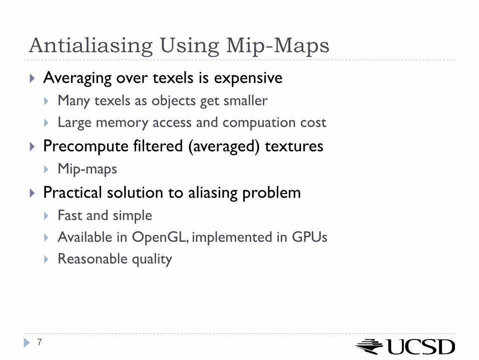
Antialiasing Using Mip-Maps Averaging over texels is expensive Many texels as objects get smaller Large memory access and compuation cost
Precompute filtered (averaged) textures Mip-maps
Practical solution to aliasing problem Fast and simple Available in OpenGL, implemented in GPUs Reasonable quality
7
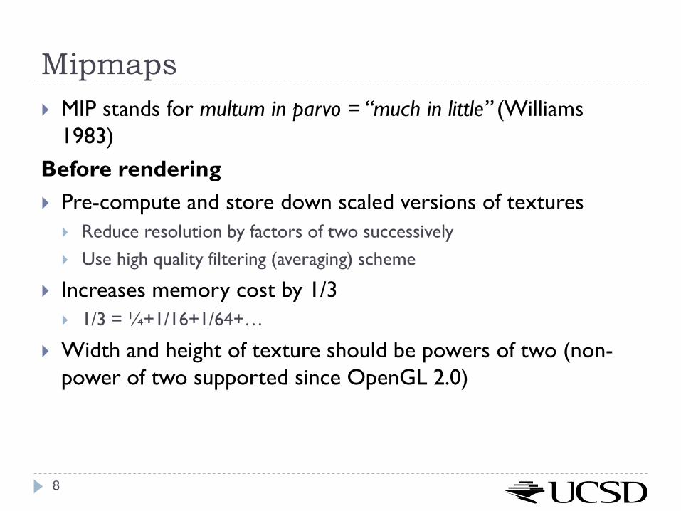
Mipmaps MIP stands for multum in parvo = “much in little” (Williams
1983)Before rendering Pre-compute and store down scaled versions of textures Reduce resolution by factors of two successively Use high quality filtering (averaging) scheme
Increases memory cost by 1/3 1/3 = ¼+1/16+1/64+…
Width and height of texture should be powers of two (non-power of two supported since OpenGL 2.0)
8

Mipmaps Example: resolutions 512x512, 256x256, 128x128, 64x64,
32x32 pixels
“multum in parvo”Level 0
Level 1
23
4
9

Mipmaps One texel in level 4 is the average of 44=256 texels in
level 0
“multum in parvo”Level 0
Level 1
23
4
10

Mipmaps
Level 0 Level 1 Level 2
Level 3 Level 411

Rendering With Mipmaps “Mipmapping” Interpolate texture coordinates of each pixel as without
mipmapping Compute approximate size of pixel in texture space Look up color in nearest mipmap E.g., if pixel corresponds to 10x10 texels use mipmap level 3 Use nearest neighbor or bilinear interpolation as before
12

MipmappingTexture spaceCamera spaceImage plane
Pixel area
Texels
Mip-map level 0Mip-map level 1Mip-map level 2Mip-map level 313

Nearest Mipmap, Nearest Neighbor Visible transition between mipmap levels
14

Nearest Mipmap, Bilinear Visible transition between mipmap levels
15

Trilinear Mipmapping Use two nearest mipmap levels E.g., if pixel corresponds to 10x10 texels, use mipmap levels 3
(8x8) and 4 (16x16)
2-Step approach: Step 1: perform bilinear interpolation in both mip-maps Step 2: linearly interpolate between the results
Requires access to 8 texels for each pixel Supported by hardware without performance penalty
16

Anisotropic Filtering Method of enhancing the image
quality of textures on surfaces that are at oblique viewing angles
Different degrees or ratios of anisotropic filtering can be applied
The degree refers to the maximum ratio of anisotropy supported by the filtering process. For example, 4:1 anisotropic filtering supports pre-sampled textures up to four times wider than tall
17

More Info Mipmapping tutorial w/source code: http://www.videotutorialsrock.com/opengl_tutorial/mipmapping/text.php
18

Environment Mapping

More Realistic Illumination In the real world:
At each point in scene light arrives from all directions Not just from a few point light sources Global Illumination is a solution, but computationally expensive
Environment Maps Store “omni-directional” illumination as images Each pixel corresponds to light from a certain direction Sky boxes make for great environment maps
20

Capturing Environment Maps Environment map = surround panoramic
image Creating 360 degrees panoramic images: 360 degree camera “light probe” image: take picture of mirror
ball (e.g., silver Christmas ornament)
Light Probes by Paul Debevechttp://www.debevec.org/Probes/
21

Environment Maps as Light SourcesSimplifying Assumption Assume light captured by environment map is emitted
from infinitely far away Environment map consists of directional light sources Value of environment map is defined for each direction,
independent of position in scene Approach uses same environment map at each point in
sceneApproximation!
22

Applications for Environment Maps Use environment map as “light source”
Global illumination withpre-computed radiance transfer
[Sloan et al. 2002]
Reflection mapping[Georg-Simon Ohm University of Applied Sciences]
23

Cubic Environment Maps Store incident light on six faces
of a cube instead of on sphere
Spherical map Cube map24

Cubic vs. Spherical Maps Advantages of cube maps: More even texel sample density
causes less distortion, allowing for lower resolution maps
Easier to dynamically generate cube maps for real-time simulated reflections
25
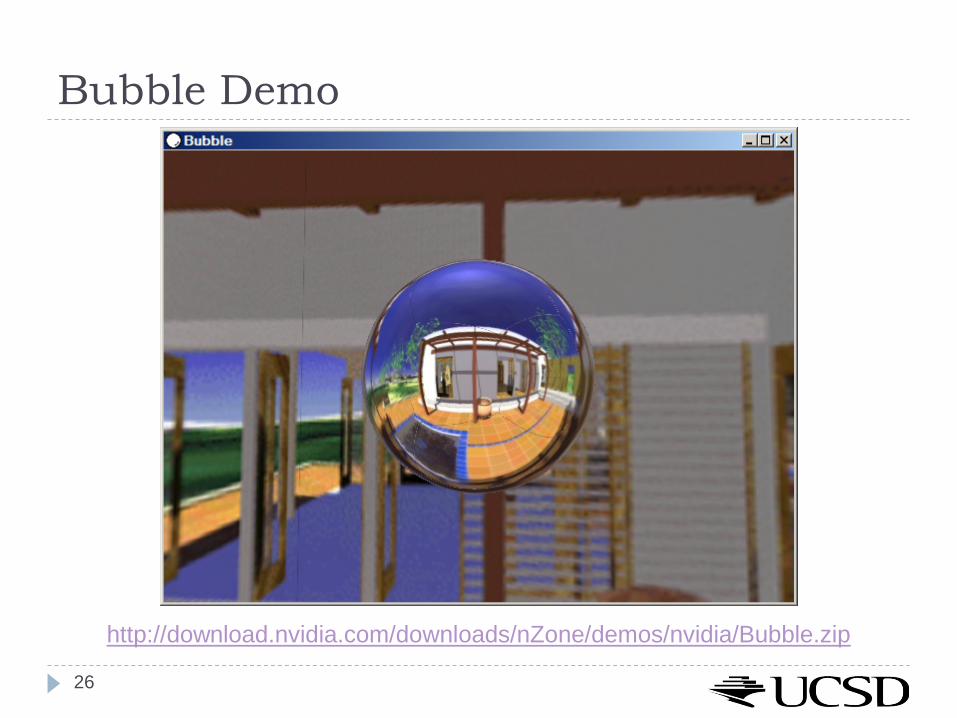
Bubble Demo
http://download.nvidia.com/downloads/nZone/demos/nvidia/Bubble.zip
26

Cubic Environment MapsCube map look-up Given: light direction (x,y,z) Largest coordinate component determines cube map face Dividing by magnitude of largest component yields
coordinates within face In GLSL: Use (x,y,z) direction as texture coordinates to samplerCube
27

Reflection Mapping Simulates mirror reflection Computes reflection vector at each pixel Use reflection vector to look up cube map Rendering cube map itself is optional (application dependent)
Reflection mapping28
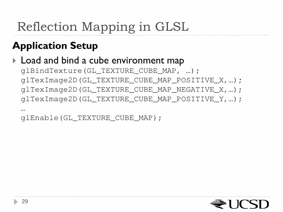
Reflection Mapping in GLSLApplication Setup Load and bind a cube environment mapglBindTexture(GL_TEXTURE_CUBE_MAP, …);glTexImage2D(GL_TEXTURE_CUBE_MAP_POSITIVE_X,…);glTexImage2D(GL_TEXTURE_CUBE_MAP_NEGATIVE_X,…);glTexImage2D(GL_TEXTURE_CUBE_MAP_POSITIVE_Y,…);…glEnable(GL_TEXTURE_CUBE_MAP);
29

Environment Mapping: Concept
30
Source: http://antongerdelan.net/opengl/cubemaps.html

Environment Mapping: Vertex Shader
31
#version 400
in vec3 vp; // positions from meshin vec3 vn; // normals from meshuniform mat4 P, V, M; // proj, view, model matricesout vec3 pos_eye;out vec3 n_eye;
void main() {pos_eye = vec3(V * M * vec4(vp, 1.0));n_eye = vec3(V * M * vec4(vn, 0.0));gl_Position = P * V * M * vec4(vp, 1.0);
}

Environment Mapping: Fragment Shader#version 400
in vec3 pos_eye;
in vec3 n_eye;
uniform samplerCube cube_texture;
uniform mat4 V; // view matrix
out vec4 frag_colour;
void main()
{
// reflect ray around normal from eye to surface
vec3 incident_eye = normalize(pos_eye);
vec3 normal = normalize(n_eye);
vec3 reflected = reflect(incident_eye, normal);
// convert from eye to world space
reflected = vec3(inverse(V) * vec4(reflected, 0.0));
frag_colour = texture(cube_texture, reflected);
}
32
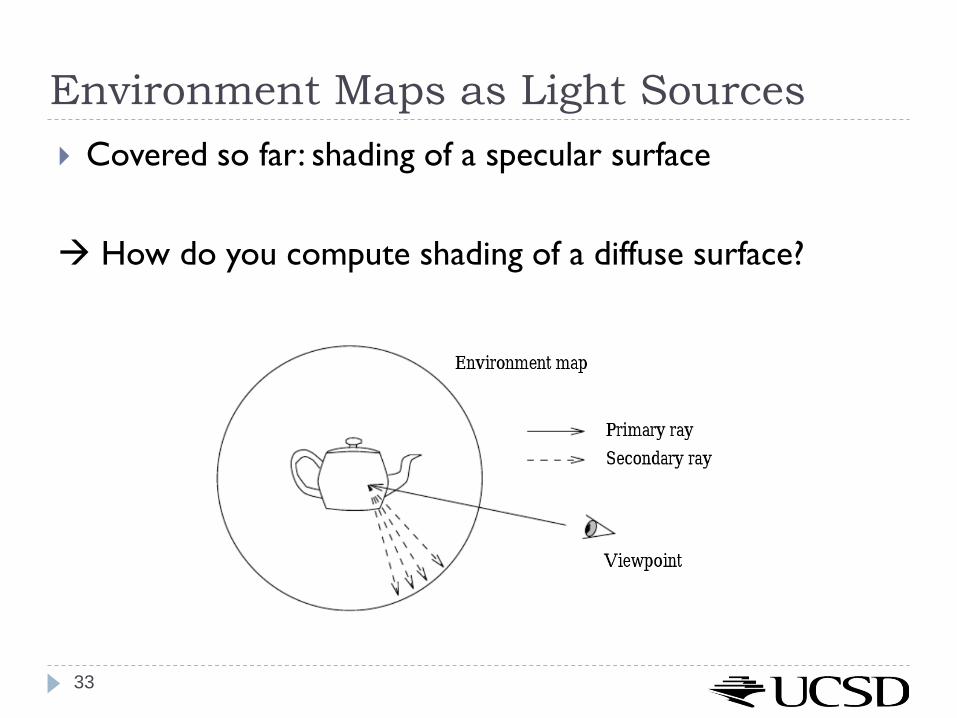
Environment Maps as Light Sources Covered so far: shading of a specular surface
How do you compute shading of a diffuse surface?
33

Diffuse Irradiance Environment Map Given a scene with k directional lights, light directions d1..dk and intensities i1..ik,
illuminating a diffuse surface with normal n and color c
Pixel intensity B is computed as:
Cost of computing B proportional to number of texels in environment map!
Precomputation of diffuse reflection
Observations: All surfaces with normal direction n will return the same value for the sum The sum is dependent on just the lights in the scene and the surface normal
Precompute sum for any normal n and store result in a second environment map, indexed by surface normal
Second environment map is called diffuse irradiance environment map
Allows to illuminate objects with arbitrarily complex lighting environments with single texture lookup
∑=
⋅=kj
jj indcB..1
),0max(
34
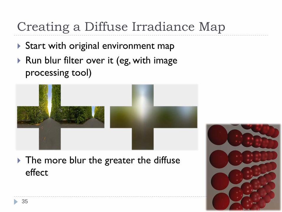
Creating a Diffuse Irradiance Map Start with original environment map Run blur filter over it (eg, with image
processing tool)
The more blur the greater the diffuseeffect
35
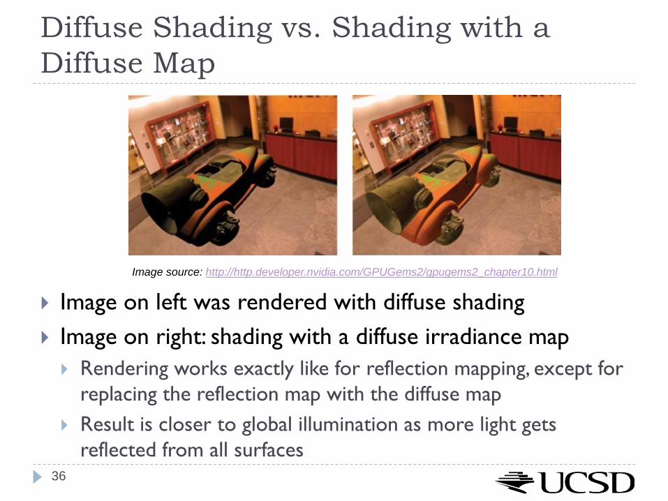
Diffuse Shading vs. Shading with a Diffuse Map
Image on left was rendered with diffuse shading Image on right: shading with a diffuse irradiance map Rendering works exactly like for reflection mapping, except for
replacing the reflection map with the diffuse map Result is closer to global illumination as more light gets
reflected from all surfaces36
Image source: http://http.developer.nvidia.com/GPUGems2/gpugems2_chapter10.html

Summary Two types of cubic environment maps: Reflection map used for mirror reflective objects Diffuse map used for less shiny objects
37
Reflection Map Diffuse Map
Top Related