Crystal Plasticity Based Finite Element Modeling in

Polycrystalline Ti-7Al Alloys

by

Chengcheng Tao

A thesis submitted to The Johns Hopkins University in conformity with the

requirements for the degree of Master of Science.

Baltimore, Maryland

August, 2014

Abstract

This thesis develops an experimentally calibrated computational model

based on crystal plasticity for the analysis of α-Ti-7Al polycrystalline alloys.

The crystal plasticity finite element model uses rate and size-dependent

anisotropic elasto plasticity constitutive law. The study contains a

combination of orientation imaging microscopy (OIM), misorientation,

microtesting, computational simulations and minimization process,

including genetic algorithms for calibration of the material parameters and

characterization. Size effects are also taken into consideration in the analysis.

The polycrystalline Ti-7Al computational model involves statistically

equivalent orientation distributions to those observed in the orientation

imaging scans. Simulations detected effects of orientation, misorientation

and microtexture distributions through simulations. Constant strain rate test

is simulated with this model, and the results are compared with experiments.

Primary Reader: Professor Somnath Ghosh

Secondary Reader: Professor Jaafar El-Awady

ii

Acknowledgements

I would like to acknowledge and thank my advisor, Dr. Somnath Ghosh,

for his encouragement, support, constructive advice, and valuable technical

training during the past 2 years. His guidance, insight, and drive were the

single largest factor in the completion of the thesis. I also appreciate

Professor El-Awady’s careful review and detailed comments for my work.

I must also thank all my colleagues at Computational Mechanics

Research Laboratory, who I continually relied upon for assistance. I would

like to particularly thank Jiahao Cheng, Ahmad Shahba for their time and

efforts in personally helping me with my project during these entire 2 years.

I owe a lot of my training in computational mechanics to their willingness to

help and mentor me even through times where they had their own work to

do.

Special thanks to Dr. Adam Pilchak from Air Force Research Laboratory

for his adequate experiment data as well as patient collaboration with us

during the project.

I also acknowledge the financial support of Army Research Laboratory

and computer support by the Homewood High Performance Compute

Cluster.

iii

Contents

Abstract ........................................................................................................... ii

Acknowledgements........................................................................................ iii

List of Tables ................................................................................................... v

List of Figures ................................................................................................ vi

Introduction ...................................................................................................... 1

Material description and model ....................................................................... 6

2.1 Material description ................................................................................ 6

2.2 Crystal plasticity constitutive model ...................................................... 7

2.2.1 Crystal plasticity based material model ........................................... 8

2.2.2 Size dependence in the crystal plasticity model for Ti-7Al ...........10

Calibration for material parameters from single crystal experiment data .....11

3.1 Mechanical testing of single α colonies in Ti-7Al microstructure .......12

3.2 Calibration process ...............................................................................14

3.3 Calibration results .................................................................................16

3D Polycrystalline microstructural simulation and mesh generation............22

4.1 Microstructural Characterization of the α Ti-7Al ................................23

4.2 Microsturctural Simulation Procedures ................................................25

4.3 Microstructural Simulation Validation .................................................34

4.4 Mesh Generation ..................................................................................34

Simulation of deformation in polycrystalline Ti-7Al ....................................37

Conclusion .....................................................................................................41

Bibliography ..................................................................................................43

Curriculum Vitae ...........................................................................................47

iv

List of Tables

3.1 Calibrated parameters for basal <a>, prismatic <a>, pyramidal <a> and

pyramidal <c+a> slip systems

3.2 Calibrated parameters for yield point phenomenon in each slip system

5.1 Calibrated parameters for polycrystalline model

v

List of Figures

2.1 HCP crystal structure and slip systems with non-orthogonal basis

3.1 Single crystal Experimental results for different slip systems and

constant strain rates.

3.2 Single crystal experimental and calibrated curved for basal <a>,

prismatic <a> and pyramidal <c+a>slip systems under different strain rate

4.1 EBSD scans of 4 orthogonal surfaces and surface after crop the edge

4.2 Grain size, D, distribution comparison

4.3 Distribution of number of contiguous neighbors

4.4 α phase (0001) and (101�0) pole figure for Sample data and Synthetic

structure data

4.5 Misorientation distribution comparison

4.6 Microtexture distribution comparison

4.7 Voxelized volumes before and after meshing for the 1000 grain

microstructure

vi

4.8 Voxelized volumes before and after meshing for the 200 grain

microstructure

5.1 Experimental and simulation stress-strain curve with Ti-7Al

polycrystalline model under constrain strain rate

vii

Chapter 1

Introduction

Titanium alloys are widely used in a number of applications from

aerospace, medical, sporting goods industries [1] because of their high

strength (~700-1000Mpa), low density, high fracture toughness and

corrosion resistance [2]. These alloys exhibit a cold creep phenomenon.

Time dependent deformation is seen to happen at room temperature and at

loads as 60% of yield strength [3-7]. The cold creep mechanism occurs due

to dislocation glide where dislocations are arrayed in a planar fashion instead

of diffusion-mediated at low homologous temperatures. It is mainly

dependent on crystallographic orientation features directly affect mechanical

properties of polycrystalline materials.

Transmission electron microscopy study has shown that deformation is

caused by dislocation glide, where the dislocations are inhomogeneously

distributed into planar arrays. The planarity of slip has been attributed to the

effect of short range ordering of Ti and Al atoms on the HCP lattice [8]. In

addition, creep strains can accumulate at applied stresses significantly

smaller than the yield strength. In this way, titanium alloys are chosen

1

widely in high performance structural applications where dimensional

tolerance is a critical factor.

Ti alloy shows rate sensitivity values typically that are similar from those

observed in other metallic alloys that do not display a similar low

temperature creep behavior [9]. It has also been recognized that crack

initiation in Ti is related with grains that have the [0 0 0 1] crystal

orientations close to the deformation axis. A number of references have been

speculated for this effect [10], which shows that local load shedding between

grains of different orientations has a significant effect on this behavior.

In pure Ti and its alloys, plastic deformation depended on the crystal

orientation considerably. These HCP materials exhibit complex modes of

deformation due to their low symmetries. The inelastic deformation is highly

anisotropic because of the difference in deformation resistances in different

slip systems of the crystals [11]. For example, single crystals α-Ti-6Al are

significantly stronger when the deformation axis is parallel to the [0 0 0 1]

direction of the crystal [10]. In this orientation, <c+a> dislocation slip on

pyramidal planes is activated. In this situation, critical resolved shear

strength (CRSS) is much larger than the CRSS for <a> dislocation slip on

basal or prismatic planes. And the planar slip causes the strain hardening

exponents of Ti alloys quite small [8]. This makes the effect of grain 2

boundaries and interfaces on deformation important. With little intrinsic

ability to strain hardening, planar slip bands propagate across favorably

oriented grains upon initial loading. Large local stress concentrations

consequently develop in neighboring grains, which are less favorably

oriented for <a>-type slip. Local stresses are particularly large when

favorably oriented with its <c>-axis parallel to the macroscopic deformation

direction [12].

The disadvantage in experiments is the large cost for processing and

testing real samples as well as varying one microstructural feature while

holding the other constant because of their highly coupled characteristics

[13]. Image-based modeling and simulation with crystal plasticity finite

element method analyses of polycrystalline microstructures is a good option

compared to experimental methods for determining microstructure-property

relationships. The models by Groeber [14] represent the characteristics of

crystallographic orientations, misorientations, grain morphology and

distributions for good predictive capability. Compared with experiment, it’s

easy to vary the microstructural features of these specimens independently to

get a direct understanding of the effect on properties. It’s important that the

models be experimentally validated and efficient for simulating a large

number of grains in the polycrystalline aggregate [15-16].

3

Rate dependent and independent crystal plasticity models have been

developed in literature to predict anisotropy due to crystallographic texture

evolution, e.g. in [17-19]. Anand et al. have developed experiment based

crystal plasticity computational models for OHFC copper (fcc) [20],

aluminum (fcc) [11] and tantalum (bcc) [21]. Curve fitting to polycrystalline

experimental data is used to obtain material parameters. By comparing its

predictions for stress-strain relation and texture evolution, the predictive

capability of the model is evaluated. Robust computational and experimental

effort for titanium (hcp) at high temperatures has also been reported by

Balasubramanian and Anand [11, 22]. Slip system data for crystal plasticity

parameters have been calibrated from single crystal experiments with

polysyntetically twinned 𝛼𝛼2 -𝑇𝑇𝑇𝑇3Al and Ti-6Al by Grujicic, Batchu and

Hasija [23]. Kad [24] have used these single crystal based parameters to

model polycrystalline material behavior.

The present thesis aims to develop a quantitative understanding of the

role of microstructure on the rate-dependent plastic response of the titanium

alloy Ti-7Al using a comprehensive CPFEM analysis based approach. The

overall process encompasses 2D microstructural characterization, 3D

microstructure model creation, mesh generation and subsequently, CPFEM

analysis and data processing. Quantitative characterization of material

4

microstructures is accomplished through SEM image analysis, EBSD data

collection, stereological procedures and statistical quantification. Subsequent

to material characterization and data acquisition, a 3D reconstruction code

developed in [14-16] is used to create statically equivalent, virtual

microstructures that are meshed for computational simulations. Crystal

plasticity finite element method simulations and analyses are conducted for

strain-rate controlled and compared with experimental results for calibrating

the model. In order to gain an understanding of sensitivities to the

microstructure, virtual microstructures with varying characteristic functions

are generated and analyzed.

5

Chapter 2

Material description and model

2.1 Material description

The material studied in this work is single-phase α-Ti-7Al which has an

HCP crystal structure. Close-packed layers of atoms are stacked in the order

ABABAB so that the hexagonal crystal structure is created. Every third

layer is in exactly the same relative position as the first. The interatomic

spacing on the A plane is denoted by a while the spacing between adjacent

A planes is denoted by c. The ratio c/a is termed the axial ratio, which is

different in different hexagonal materials. Titanium has an axial ratio of

c/a=1.587.

The material basis vectors corresponding to the HCP lattice structure are

denoted by a set of nonorthogonal base vectors, {𝐚𝐚𝟏𝟏,𝐚𝐚𝟐𝟐,𝐚𝐚𝟑𝟑, 𝐜𝐜}, with 𝐚𝐚𝟏𝟏 +

𝐚𝐚𝟐𝟐 + 𝐚𝐚𝟑𝟑 = 0, as shown Fig.1. For computational simplicity, an orthonormal

basis {𝐞𝐞1c ,𝐞𝐞2c ,𝐞𝐞3c} can be derived from these crystallographic vectors [11].

The HCP crystals are made of five different families of slip systems, which

are the basal <a>, prismatic <a>, pyramidal <a>, first order pyramidal <c+a>

and second order pyramidal <c+a> slip systems with a total of 30 slip

6

system, as shown in Fig 2.1. For elasticity, a transversely isotropic response

with five independent elastic constants is used to model the anisotropy [11].

(a) (b) (c)

3 Basal-<a> 3 Prismatic-<a> 6 Pyramidal-<a>

{0001}<112�0> {101�0}<1120> {101�1}<112�0>

(d) (e)

12 1st order Pyramidal-<c+a> 6 2nd order Pyramidal-<c+a>

{101�1}<112�3> {112�2}<112�3>

Fig. 2.1 HCP crystal structure and slip systems with non-orthogonal basis.

Figure is taken form Balasubramanian [11]

2.2 Crystal plasticity constitutive model 7

2.2.1 Crystal plasticity based material model

The deformation behavior of Ti-7Al is modeled using a rate-dependent,

finite strain, crystal plasticity formulation, which is isothermal, elastic-

viscoplastic. In this model, crystal deformation is caused by the elastic

stretching and rotation of the crystal lattice and plastic slip on the different

slip system.

The stress-strain relation in this model is written in terms of the second

Piola-Kirchoff stress (S=det𝐅𝐅e𝐅𝐅e−1σ𝐅𝐅e−T) and the work conjugate Lagrange

Green strain tensor (𝐄𝐄e ≡ (1/2){𝐅𝐅eT𝐅𝐅e − 𝐈𝐈}) as

S=C:𝑬𝑬𝑒𝑒 (1)

where C is a fourth order anisotropic elasticity tensor, σ is the Cauchy stress

tensor and 𝐅𝐅e is an elastic deformation gradient defined by the relation

𝐅𝐅e ≡ 𝐅𝐅𝐅𝐅p−1, det𝐅𝐅e > 0 (2)

𝐅𝐅 and 𝐅𝐅p are the deformation gradient and its plastic component,

respectively, with the incompressibility constraint det𝐅𝐅p=1. The flow rule

governing evolution of plastic deformation is expressed as in terms of the

plastic velocity gradient

𝐋𝐋p = �̇�𝐅p𝐅𝐅p−1 = ∑ �̇�𝛾α𝐬𝐬0αα (3) 8

where the Schmidt tensor is expressed as 𝐬𝐬0α ≡ 𝐦𝐦0α ⊗ 𝐧𝐧0α in terms of the slip

direction (𝐦𝐦0α) and slip plane normal (𝐧𝐧0α) in the reference configuration,

associated with the αth slip system. The plastic shearing rate �̇�𝛾α on the αth

slip system is given by the power law relation:

�̇�𝛾α = 𝛾𝛾�̇ �𝜏𝜏𝛼𝛼

𝑔𝑔𝛼𝛼�1/𝑚𝑚

𝑠𝑠𝑇𝑇𝑠𝑠𝑠𝑠(𝜏𝜏𝛼𝛼), 𝜏𝜏𝛼𝛼 ≡ (𝐂𝐂e:𝐒𝐒) ∙ 𝐬𝐬0𝛼𝛼 (4)

𝛾𝛾�̇ is the reference plastic shearing rate, 𝜏𝜏𝛼𝛼 and 𝑠𝑠𝛼𝛼are the αth slip system

resolved shear stress and the slip system deformation resistance. m is the

material rate sensitivity parameter and 𝐂𝐂e is the elastic stretch. The slip

system resistance is taken to evolve as:

�̇�𝑠α = ∑ ℎ𝛼𝛼𝛼𝛼��̇�𝛾β�𝑛𝑛𝑛𝑛𝑛𝑛𝑛𝑛𝑛𝑛𝛼𝛼=1 = ∑ 𝑞𝑞𝛼𝛼𝛼𝛼ℎ𝛼𝛼𝛼𝛼 (5)

where ℎ𝛼𝛼𝛼𝛼 is the strain hardening rate due to self and latent hardening, ℎ𝛼𝛼 is

self-hardening rate and 𝑞𝑞𝛼𝛼𝛼𝛼 is a matrix describing the latent hardening. The

evolution of the self-hardening rate is governed by the relation:

ℎ𝛼𝛼 = ℎ0𝛼𝛼 �1 − 𝑔𝑔𝛽𝛽

𝑔𝑔𝑠𝑠𝛽𝛽� sign(1 − 𝑔𝑔𝛽𝛽

𝑔𝑔𝑠𝑠𝛽𝛽), 𝑠𝑠𝑛𝑛

𝛼𝛼 = 𝑠𝑠�(�̇�𝛾𝛽𝛽

𝛾𝛾�̇)𝑛𝑛 (6)

where ℎ0 is the initial hardening rate, 𝑠𝑠𝑛𝑛𝛼𝛼 is the saturation slip deformation

resistance, and r, 𝑠𝑠� and n are the slip system hardening parameters.

9

2.2.2 Size dependence in the crystal plasticity model for Ti-7Al

In continuum plasticity, the dependence of the flow stress on the grain

size has been expressed by the Hall-Petch relationship in [13, 25]. In crystal

plasticity formulation, a similar equation that relates the slip system

deformation resistance gα to a characteristic size can be expressed as

gα = g0α + Kα

√𝐷𝐷α (7)

where g0α and Kα are size-effect-related slip system constants that refer to

the interior slip system deformation resistance and slope, respectively, and

Dα is the characteristic length scale governing the size effect. The

characteristic length scale (Dα) for a single-phase alloy is represented by the

average grain size. The crystal plasticity parameters, calibrated for single

crystal α Ti-6Al [12], are used in the present for the primary α phase.

Experiments on single crystal α-Ti-7Al have been used in Hasija [12]

(2003) to calibrate crystal plasticity parameters for individual slip systems in

each of the constituent phases by a genetic algorithm [12, 26, 27] based

optimization scheme. The calibrated values of the initial slip system

10

deformation resistance 𝑠𝑠𝛼𝛼 reflect the anisotropy caused by the basal,

prismatic and pyramidal slip systems.

Chapter 3

Calibration for material parameters from single crystal

experiment data

11

3.1 Mechanical testing of single α colonies in Ti-7Al

microstructure

The computational models in this thesis are calibrated and validated

using results of mechanical tests, conducted with samples of single-phase 𝛼𝛼-

Ti-7Al. The single crystal experimental results are provided by Adam

Pilchak from Air Force Research Labs. Tension tests are conducted with

single crystals, in which samples are each oriented to maximize the resolved

shear stress on one of the three <a>-type slip directions on the prismatic and

basal planes. In addition, tests are conducted with samples for which the [0 0

0 1] axis coincides with the tensile direction.

All single α colonies of Ti-7Al samples for mechanical testing are

extracted from successfully grown colonies ranging in size from 5 to 25 mm.

Laue back-reflection X-ray techniques are used to identify the

crystallographic orientation of the α phase. Scanning electron microscopy

(SEM) observations are used to determine the relative alignment of the

broad face of the α interface, allowing for the unambiguous identification of

the three a-type {1120} slip directions. A plunge electrical discharge

machining process is used to extract dogbone-shaped microtensile samples

from the thin oriented single-crystal sections. Microtensile testing of these

12

samples is performed in a piezo-driven microsample testing machine. Nine

tests are conducted at constant strain rates of 1.7× 10−4 , 5.2× 10−4 ,

9.7×10−4 𝑠𝑠−1 with maximum slip activity on the basal, prismatic, and <c+a>

pyramidal slip systems. The experimental results are shown as Fig 3.1.

(a)

(b)

13

(c)

Fig.3.1 Single crystal Experimental results for different slip systems and

constant strain rates. (a) <a> basal slip system, (b) <a>prismatic slip system,

<c+a> pyramidal slip system.

3.2 Calibration process

The calibration for single crystal includes anisotropic elastic constants

and crystal plasticity parameters in each crystal. For calibration purpose,

constants strain rate uniaxial tensile tests at rate of 10−4 𝑠𝑠−1 are conducted

with single crystal α-Ti-7Al alloys. Three experiments are set up for

maximum slip system activity (maximum Schmid factor) along the basal

<a>, prismatic <a> and pyramidal <c+a> slip system, respectively. 1296

four-noded tetrahedron elements are used in the single crystal calibration.

14

The elastic-plastic constitutive relation for finite deformation is incorporated

with the UMAT user interface. Displacement boundary condition is applied

on the top surface and nodes on the bottom are fixed.

The elastic constants are calibrated by comparing the slope of the

experimental stress-strain curve in the constant strain rate test for single

crystals with that obtained from the finite element simulations. The material

coordinate system is defined by orthonormal basis{𝐞𝐞1𝑐𝑐 ,𝐞𝐞2𝑐𝑐 ,𝐞𝐞3𝑐𝑐}, where the 1, 2,

3 directions are aligned with the [1� 2 1� 0], [1� 0 1 0] and [0 0 0 1] directions

of the HCP crystal lattice, respectively. In this system, the components of the

elastic stiffness tensor 𝐶𝐶𝛼𝛼𝛼𝛼(α=1,…,6, β=1,…,6) for a transversely isotropic

material are determined from the experiment observations to be:

𝐶𝐶11=𝐶𝐶22=165.49 Gpa, 𝐶𝐶12=114.23 Gpa, 𝐶𝐶13=𝐶𝐶23=66.303 Gpa, 𝐶𝐶33=208.23

Gpa, 𝐶𝐶44=25.63 Gpa, 𝐶𝐶55= 𝐶𝐶66=65.828 Gpa and all other 𝐶𝐶𝛼𝛼𝛼𝛼’s=0.

Due to the number of parameters required to describe the slip system

flow rule, shear resistance relation and the nonlinearity of these equations,

genetic algorithm [12, 26, 27] is used in the process of optimization. Of the

various parameters calibrated using the experimental results are (i) material

rate sensitivity m, (ii) the reference plastic shearing rate 𝛾𝛾�̇, (iii) the initial

15

slip system deformation resistance 𝑠𝑠0𝛼𝛼, (iv) the initial hardening rate ℎ0 and

(v) various shear resistance evolution related parameters r, 𝑠𝑠� and n.

Material parameter calibration is conducted in two stages. In the first

step, a sensitivity analysis is conducted to determine which parameters affect

the response significantly. The key response variables are considered to be

the proportional limit (𝜎𝜎𝑛𝑛), initial macroscopic yield strength (𝜎𝜎𝑦𝑦), and the

post yield slope (H) in the stress-strain curve. For 𝜎𝜎𝑛𝑛 and 𝜎𝜎𝑦𝑦 , higher

sensitivity is observed with respect to m, 𝛾𝛾�̇, 𝑠𝑠0𝛼𝛼. And for H, high sensitivity

is observed with respect to 𝛾𝛾�̇, 𝑠𝑠0𝛼𝛼, ℎ0, 𝑠𝑠�. High sensitivity is associated with a

higher order representation in the minimization.

The second step is the minimization of a suitably chosen objective

function with respect to the design variables to obtain parameters for the

crystal plasticity constitutive equations for the different hcp slip systems.

3.3 Calibration results

The corresponding calibrated parameters for the three different slip

systems are shown in Table 3.1.

16

Table 3.1 Calibrated parameters for basal <a>, prismatic <a>, pyramidal<a>

and pyramidal <c+a>slip systems

Parameters Basal <a>

slip system

Prismatic <a>

slip system

Pyramidal

<a> slip

system

Pyramidal

<c+a>slip

system

m 0.15 0.15 0.15 0.02

𝑠𝑠0(MPa) 327 326 500 1000

𝛾𝛾�̇(𝑠𝑠−1) 0.005 0.002 0.002 0.006

ℎ0 500 300 500 600

17

r 0.5 0.5 0.5 0.1

n 0.1 0.1 0.1 0.01

𝑠𝑠�(MPa) 500 600 750 1650

In order to simulate the yield point phenomenon in basal and prismatic

experiment result, an expression for 𝛾𝛾�̇ for HSLA steel [26] is added as a

function of plastic strain:

𝛾𝛾�̇ = �̇�𝛾0 �tanh�𝐾𝐾∗�𝜀𝜀𝑝𝑝����−𝑛𝑛𝑝𝑝��+𝑡𝑡𝑡𝑡𝑛𝑛ℎ�𝐾𝐾𝑛𝑛𝑝𝑝�

tanh(𝐾𝐾)+tanh (𝐾𝐾𝑛𝑛𝑝𝑝)� (8)

where 𝜀𝜀𝑛𝑛��� is the equivalent plastic strain defined as 𝜀𝜀𝑛𝑛��� = �23𝜀𝜀𝑛𝑛𝑖𝑖𝑛𝑛𝜀𝜀𝑛𝑛𝑖𝑖

𝑛𝑛 , and the

Lagrangian plastic strain is defined as 𝜀𝜀𝑛𝑛𝑖𝑖𝑛𝑛 = 1

2(𝐹𝐹𝑛𝑛𝑖𝑖

𝑛𝑛𝑇𝑇𝐹𝐹𝑛𝑛𝑖𝑖𝑛𝑛 − 𝛿𝛿𝑛𝑛𝑖𝑖). Equation (8)

assumes that 𝛾𝛾�̇ is the same for all slip systems initially. It increases rapidly

with plastic strain. 𝐾𝐾 and 𝑙𝑙𝑛𝑛 are material constants in this equation.

Table 3.2 Calibrated parameters for yield point phenomenon in each slip

system

Slip system �̇�𝛾0 𝐾𝐾∗ 𝑙𝑙𝑛𝑛 𝐾𝐾

18

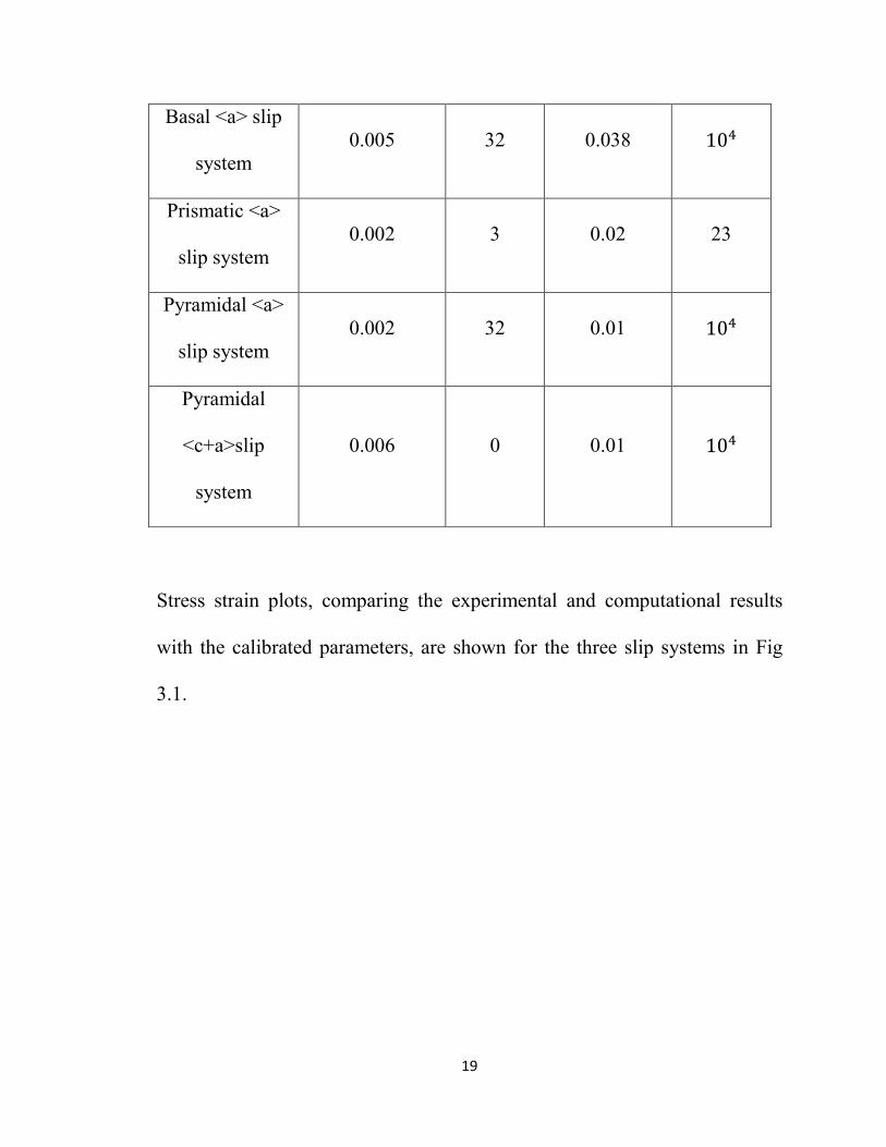
Basal <a> slip

system 0.005 32 0.038 104

Prismatic <a>

slip system 0.002 3 0.02 23

Pyramidal <a>

slip system 0.002 32 0.01 104

Pyramidal

<c+a>slip

system

0.006 0 0.01 104

Stress strain plots, comparing the experimental and computational results

with the calibrated parameters, are shown for the three slip systems in Fig

3.1.

19

(a)

(b)

20

(c)

Fig 3.2 Experimental and calibrated curved for (a) basal <a>, (b) prismatic

<a> and (c) pyramidal <c+a>slip systems under different strain rate.

However, due to the different rate sensitivity of single and

polycrystalline crystal experiment data, the single calibration results could

not be used directly for polycrystalline materials. They could be used as a

start point in the polycrystalline calibration.

21

Chapter 4

3D Polycrystalline microstructural simulation and mesh

generation

This chapter discusses the 2D characterization and generation of 3D

microstructure models from the 2D data. It has been shown that 3D

microstructures can be collected by a number of techniques, such as Focused

Ion Beam (FIB) sectioning [15], manual polishing [28] and x-ray methods

[29]. But all these methods are somehow tedious and time consuming. The

22

work here will be based on extrapolation 2D measurements to estimate 3D

statistics. This area is known as stereology, which has been under

investigation for years [30], and will serve more recent direct 3D techniques

to inform the process used in this work.

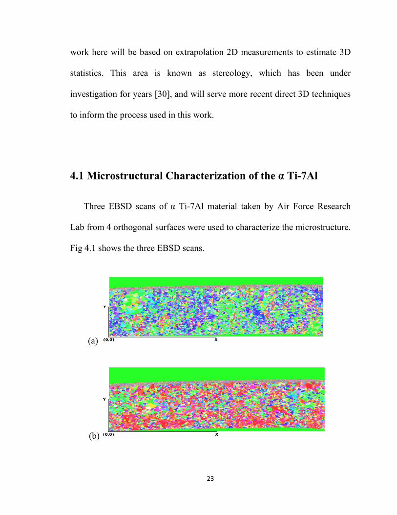
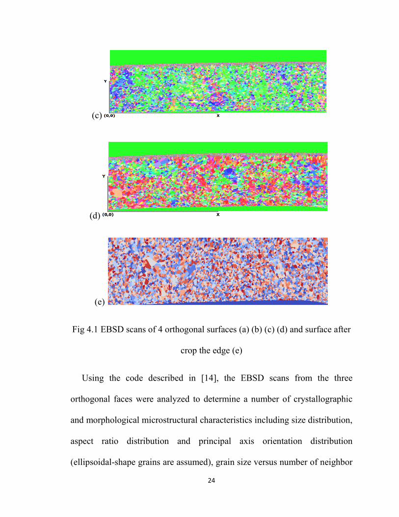
4.1 Microstructural Characterization of the α Ti-7Al

Three EBSD scans of α Ti-7Al material taken by Air Force Research

Lab from 4 orthogonal surfaces were used to characterize the microstructure.

Fig 4.1 shows the three EBSD scans.

(a)

(b)

23

(c)

(d)

(e)

Fig 4.1 EBSD scans of 4 orthogonal surfaces (a) (b) (c) (d) and surface after

crop the edge (e)

Using the code described in [14], the EBSD scans from the three

orthogonal faces were analyzed to determine a number of crystallographic

and morphological microstructural characteristics including size distribution,

aspect ratio distribution and principal axis orientation distribution

(ellipsoidal-shape grains are assumed), grain size versus number of neighbor

24

distribution, crystallographic orientation distribution, misorientation

distribution and microtexture distribution.

4.2 Microsturctural Simulation Procedures

In order to generate a representative synthetic microstructure that is

statistically equivalent to the real microstructure, the microstructural

simulation is performed using the code describe in [14].

Grain size is defined by the equivalent sphere diameter (ESD). ESD is

determined by first calculating equivalent circle diameters (ECD) using

image analysis techniques along with the assumption that the grains are

spherical in 3D space and therefore their size can be approximated by the

following stereological formula which connects the 𝐸𝐸𝐶𝐶𝐸𝐸������ of a sample with

the 𝐸𝐸𝐸𝐸𝐸𝐸������ of a sample:

𝐸𝐸𝐸𝐸𝐸𝐸������ =4π𝐸𝐸𝐶𝐶𝐸𝐸������

According to [15], the lognormal standard probability density function

provides a reasonable fit to the grain size data. This function is defined by

two parameters, average and standard deviation. For these reasons, the

25

lognormal standard distribution will be used in this work (see Fig. 4.2) and

will be sampled in the synthetic microstructure generation technique to

produce statistically equivalent synthetic structures.

In addition to the morphological analysis, the sample of Ti-7Al was

analyzed crystallographically. Crystallographic orientation data was

obtained through an EBSD scan containing about 10000 grains. Fig. 4.2

provides distribution of size with the number fraction of grains. Fig 4.3

provides the number of neighbors as a function of grain diameter. Fig 4.4

provides HCP orientation with MTEX. as well as misorientation and

microtexture distribution. Misorientation is defined from the 2D EBSD scan

along the grain boundary length but assumed as equivalent to a grain

boundary surface area in the 3D synthetic structure generation. This

assumption is reasonable in that matching is done based on a unitless

fracture obtained by normalizing the data by either total grain boundary

length (in 2D) or total grain boundary surface area (in 3D).

Misorientaton serves as a quantifiable measure of two neighboring voxels

orientation difference. The value of misorientation is given by the following

equation:

θ=min �cos−1(𝑡𝑡𝑡𝑡(𝑔𝑔𝐴𝐴𝑔𝑔𝐵𝐵𝑂𝑂)−12

)�

26

where 𝑠𝑠𝐴𝐴and 𝑠𝑠𝐵𝐵are the rotation matrics of voxel A and B and are given by:

𝑠𝑠𝑛𝑛

= �𝑐𝑐𝑐𝑐𝑠𝑠𝜑𝜑1𝑐𝑐𝑐𝑐𝑠𝑠𝜑𝜑2 − sin𝜑𝜑1𝑠𝑠𝑇𝑇𝑠𝑠𝜑𝜑2𝑐𝑐𝑐𝑐𝑠𝑠Ф 𝑠𝑠𝑇𝑇𝑠𝑠𝜑𝜑1𝑐𝑐𝑐𝑐𝑠𝑠𝜑𝜑2 + cos𝜑𝜑1𝑠𝑠𝑇𝑇𝑠𝑠𝜑𝜑2𝑐𝑐𝑐𝑐𝑠𝑠Ф 𝑠𝑠𝑇𝑇𝑠𝑠𝜑𝜑2𝑠𝑠𝑇𝑇𝑠𝑠Ф−𝑐𝑐𝑐𝑐𝑠𝑠𝜑𝜑1𝑠𝑠𝑇𝑇𝑠𝑠𝜑𝜑2 − sin𝜑𝜑1𝑐𝑐𝑐𝑐𝑠𝑠𝜑𝜑2𝑐𝑐𝑐𝑐𝑠𝑠Ф −𝑠𝑠𝑇𝑇𝑠𝑠𝜑𝜑1𝑠𝑠𝑇𝑇𝑠𝑠𝜑𝜑2 + cos𝜑𝜑1𝑐𝑐𝑐𝑐𝑠𝑠𝜑𝜑2𝑐𝑐𝑐𝑐𝑠𝑠Ф 𝑐𝑐𝑐𝑐𝑠𝑠𝜑𝜑2𝑠𝑠𝑇𝑇𝑠𝑠Ф

𝑠𝑠𝑇𝑇𝑠𝑠𝜑𝜑1𝑠𝑠𝑇𝑇𝑠𝑠Ф −𝑐𝑐𝑐𝑐𝑠𝑠𝜑𝜑2𝑠𝑠𝑇𝑇𝑠𝑠Ф 𝑐𝑐𝑐𝑐𝑠𝑠Ф�

where (𝜑𝜑1,Ф,𝜑𝜑2 ) are the Euler angles of the voxel. O is the symmetry

operator, which is a set of 3×3 matrices that account for the symmetry of the

crystal. There are 24 matrices for the cubic system of the IN100 material

used

27

Fig. 4.2 Grain size, D, distribution comparison. 𝑁𝑁𝑓𝑓 is the number fraction of

grains/colonies.

28

Fig. 4.3 Distribution of number of contiguous neighbors.

29

(a) (b)

(c) (d)

(e)

Fig. 4.4 𝛼𝛼 phase (0001) and (101�0) pole figure for (a) Sample data and (b)

Synthetic structure with 200 gains (c) Synthetic structure with 500 gains (d)

Synthetic structure with 800 gains (e) Synthetic structure with 1000 gains

30

Fig 4.5 Misorientation distribution (MoDF) comparison. Fracture

corresponds to either grain boundary length fraction or grain boundary

surface area fraction

31

Fig 4.6 Microtexture distribution comparison where microtexture is defined

by the number fraction of neighbors with misorientation less than 15。.

The microstructural simulation is performed using the code described in

[14] where statistically equivalent microstructures are generated whose

morphological and crystallographic statistics are matched. The

morphological orientation of the elongated grains was assumed to be random.

Grains are placed in the synthetic structure based on neighborhood

constraints assuming an average number of neighbors to be approximately

14 grains with a variation according to grain size. This choice was based on

32

the analysis of IN100 in [16] in 3D, where it was seen that the number of

neighbors of a grain correlated strongly to its size. This assumption of

correlation between the number of neighbors of a grain to its size implies a

lack of clustering of similarly sized grains, which appears to be valid when

viewing the 2D micrographs. After the morphological voxelized structure

has been built, the grains are assigned HCP orientations based on a random

sampling from the ODF. Misorientation and microtexturing statistics are

matched by an iterative process. Orientations are allowed to switch between

grains or be replaced by new orientation all the while the error is tracked and

compared to sample statistics until convergence is attained.

DREAM 3D is used to do the 3D microstructure reconstruction from 2D

ang file tested by Dr. Adam Pilchak from Air Force Research Lab. In the

first step, ang file is imported into .h5ebsd file which give 2D images (Fig

4.1). In the second step, bad data of the grain is filled out by finding cell

quaternions and setting misorientation tolerance and minimum allowed

defect size. In the third step, statistics law is added into distribution fitting.

For size and neighborhood distribution, log normal fit is inserted and for

aspect ratio and omega 3 distribution, beta fit is inserted. Then from the

results of step 2, the characteristics of 2D EBSD data such as size, number

of neighbors and Euler angle for each grain could be offered. In this way, we

33

could get the statistic law for size, neighbors, orientation, misorientation,

microtexture (Fig 4.2, 4.3, 4.4, 4.5, 4.6). In step 4, synthetic process is

undertaken from statistics law from step 3 by finding field phases, surface

fields, field neighbors and matching crystallography.

4.3 Microstructural Simulation Validation

The microstructural simulation procedure is validated through comparing

the sample statistics with the statistics of the simulated microstructure. Fig.

4.2, 4.3, 4.4, 4.5, 4.6 show statistics of a 200 grain, 500 grain, 800 grain,

1000 grain structure. It has been seen that by 200 grains these statistics have

converged to a small error. Structure of 200 grains and above show only

slight improvement and because large structures become computationally

very expensive, structures of between 200 grains were chosen for the current

work.

4.4 Mesh Generation

The resultant 3D microstructure model is a voxelized volume with

individual grains having a phase identification and an orientation defined by

34

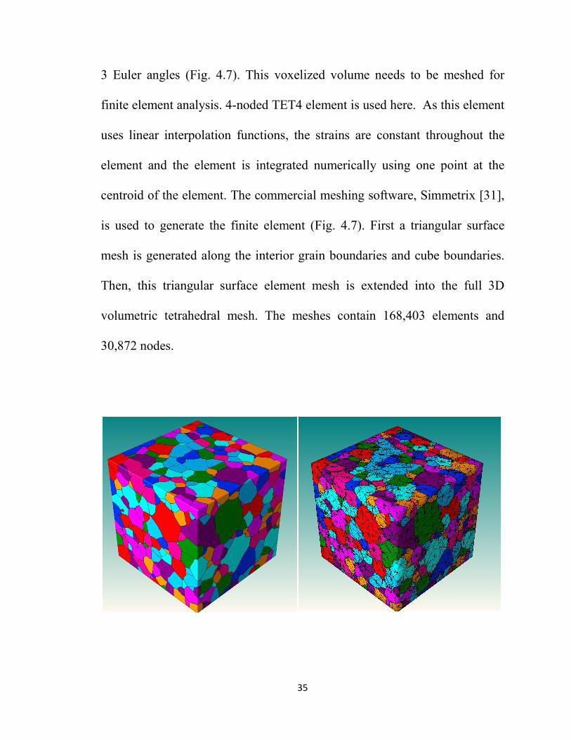
3 Euler angles (Fig. 4.7). This voxelized volume needs to be meshed for

finite element analysis. 4-noded TET4 element is used here. As this element

uses linear interpolation functions, the strains are constant throughout the

element and the element is integrated numerically using one point at the

centroid of the element. The commercial meshing software, Simmetrix [31],

is used to generate the finite element (Fig. 4.7). First a triangular surface

mesh is generated along the interior grain boundaries and cube boundaries.

Then, this triangular surface element mesh is extended into the full 3D

volumetric tetrahedral mesh. The meshes contain 168,403 elements and

30,872 nodes.

35

Fig. 4.7 Voxelized volumes before and after meshing for the 1000 grain

microstructure. The cube length dimension, 𝑙𝑙0, is 1250 μm.

The meshes are checked for distorted elements, which have a very small

number of elements with aspect ratio of 80. However because of the expense

for computation and the convergence analysis above, 200 grain

microstructure (Fig. 4.8) is used in current work for polycrystalline

calibration.

Fig. 4.8 Voxelized volumes before and after meshing for the 200 grain

microstructure. The cube length dimension, 𝑙𝑙0, is 600 μm.

36

Chapter 5

Simulation of deformation in polycrystalline Ti-7Al

Constant strain rate test is with strain rate of 4.8×10−4𝑠𝑠−1 by Dr. Adam

Pilchak from Air Force Research Lab. The overall hardening in the

polycrystalline Ti-7Al alloy is found to be low. This is attributed to the

planar slip due to the presence of short range ordering of Ti and Al atoms,

which reduces the rate of hardening as well as the interaction between the

different slip systems.

An isothermal, size-dependent and rate-dependent crystal plasticity finite

element computational model described and developed in [12, 32, 33] is

used with a parallelized code to simulate the response of synthetically

generated microstructures of the α-Ti-7Al under constrain strain rate

boundary condition.

For simulation of the constant strain rate tests, the engineering strain

rate boundary condition is applied. Consistent with the constant engineering

strain rate 𝜀𝜀�̇�𝑐 , a displacement boundary condition is applied on the right

surface of the cube as

u(t)=𝑙𝑙0(𝜀𝜀�̇�𝑐𝑡𝑡)

37

where 𝑙𝑙0 is the initial dimension (=600 μm) of the cube. The average stress-

plastic strain response in the direction of the applied displacement (𝑋𝑋2) is

plotted in Fig. 5.1. The average stress (𝜎𝜎�22) and average plastic strain (𝜀𝜀2̅2𝑛𝑛 )

are calculated as

𝜎𝜎� =∑ ∑ (𝜎𝜎22𝐽𝐽)𝑖𝑖𝑖𝑖

𝑛𝑛𝑝𝑝𝑛𝑛𝑖𝑖=1

𝑛𝑛𝑛𝑛𝑛𝑛𝑖𝑖=1

∑ ∑ (𝐽𝐽)𝑖𝑖𝑖𝑖𝑛𝑛𝑝𝑝𝑛𝑛𝑖𝑖=1

𝑛𝑛𝑛𝑛𝑛𝑛𝑖𝑖=1

, 𝜀𝜀̅ =∑ ∑ (𝜎𝜎22𝐽𝐽)𝑖𝑖𝑖𝑖

𝑛𝑛𝑝𝑝𝑛𝑛𝑖𝑖=1

𝑛𝑛𝑛𝑛𝑛𝑛𝑖𝑖=1

∑ ∑ (𝐽𝐽)𝑖𝑖𝑖𝑖𝑛𝑛𝑝𝑝𝑛𝑛𝑖𝑖=1

𝑛𝑛𝑛𝑛𝑛𝑛𝑖𝑖=1

where 𝜎𝜎22 and 𝜀𝜀22𝑛𝑛 are the Cauchy stress and the true strain at each element

integration point and J is the determinant of the Jacobian matrix at these

integration points. The number of elements in the model is designed as nel,

and npt corresponds to the number of integration points per element.

Single crystal calibration result in Chapter 3 is used as the starting point

for polycrystalline calibration. The plot in Fig. 5.1 compares the

experimental and the computational result for the constant engineering strain

rate 4.8×10−4𝑠𝑠−1. And calibrated parameters for polycrystalline model is

shown in Table 5.1

38

Table 5.1 Calibrated parameters for polycrystalline model

Parameters Basal <a>

slip system

Prismatic <a>

slip system

Pyramidal

<a> slip

system

Pyramidal

<c+a>slip

system

m 0.15 0.15 0.15 0.02

𝑠𝑠0(MPa) 220 220 330 560

𝛾𝛾�̇(𝑠𝑠−1) 0.005 0.002 0.002 0.006

ℎ0 500 300 500 600

r 0.5 0.5 0.5 0.1

n 0.1 0.1 0.1 0.01

𝑠𝑠�(MPa) 500 600 750 1650

39

Fig 5.1 Experimental and simulation stress-strain curve with Ti-7Al

polycrystalline model under constant strain rate 4.8×10−4𝑠𝑠−1

Fig. 5.1 shows the comparison for the tensile constant strain rate test. The

yield stress is about 680 Mpa. The finite element model is able to capture the

behavior of polycrystalline Ti-7Al well. Considering variabilities in the

model and the range of time over which the experiments are conducted, the

agreement between the experimental and simulated results is good.

40

Chapter 6

Conclusion

This project is aimed at a systematic development of an experimentally

validated crystal plasticity based computationally model of α-Ti-7Al. A rate-

dependent crystal plasticity model is incorporated in this model to

accommodate anisotropy in material behavior. Ti-7Al only consists of one α

phase. A set of behavior including micro testing, computational simulations,

and minimization process is implemented in this study for characterization

and calibration of material parameters. Elastic and crystal plasticity

parameters for crystal slip systems are determined by this process. Then the

polycrystalline computational model for Ti-7Al is constructed to incorporate

accurate phase volume fractions, and orientation distributions that are

statistically equivalent to those observed in OIM scans. The effects of

accurate orientation, misorientations and microtexture distributions are

investigated through simulations using this computational model. The

polycrystalline finite element model is calibrated by comparing the results of

simulations with experimental data on constant strain rate.

The capability of this model in capturing microstructural stress-strain

evolution is good. In the future work, two particular effects-local orientation

41

distributions and load shedding, will be investigated. The stress in the

loading direction and that normal to the basal plane are important variables

governing dwell fatigue crack initiation that are examined. Tests with

different constant strain rates and loading direction will be simulated to

validate the model. And creep test will also be simulated and compared with

experiments. This thesis provides a good understanding of Ti-7Al from a

local viewpoint and provides the potential for its being used for developing

fatigue failure criteria.

42

Bibliography

[1] Froes FH, editor. Non-aerospace applications of titanium. Warrendale

(PA): TMS; 1998.

[2] Donachie Jr MJ. Titanium-a technical guide. Metals Park (OH): ASM

International, 1998.

[3] Adenstedt HK. Metal. Progress 1949; 65: 658.

[4] Inman MA, Gilmore CM. Metall. Trans. 1979; 10:419.

[5] Chu HP. J. Mater. 1970; 5:633.

[6] Odegard BC, Thompson AW. Metall. Trans. 1974; 5:1207.

[7] Miller WH, Chen RT, Starke EA. Metall. Trans. 1987; 18A:1451.

[8] Neeraj T, Mills MJ. Mat. Sci Eng. A-Struct. 2001; 319:415.

[9] Neeraj T, Hou DH, Daehn GS, Mills MJ. Acta Mater. 2000; 48: 1225.

[10] Paton NE, Baggerly RG, Williams JC. AFOSR Report SC526.7FR.

1976.

43

[11] Balasubramanian S. Polycrystalline plasticity: application to

deformation processing of lightweight metals. PhD. dissertation. Cambridge

(MA): MIT; 1998.

[12] Hasija V, Ghosh S, Mills MJ, Joseph DS. Acta Mater 2003;51:4533.

[13] Hall EO. Proc Phys Soc London 1951;64:747.

[14] M. Grober. Development of an automated characterization-

representation framework for the modeling of polycrystalline materials in

3D. PhD thesis, The Ohio State University, 201 West 19th Avenue,

Columbus, OH 43210, 2007.

[15] M. Groeber, B.K. Haley, M.D. Uchic, D.M. Dimiduk, and S. Ghosh.

Materials Characterization, 57:259-273, 2006.

[16] M. Groeber, S. Ghosh, M. Uchic, and D. Dimiduk. Acta Materialia,

56:1257-1273, 2008.

[17] Peirce D, Asaro RJ, Needleman A. Acta Metall. Mater. 1983; 31:1951.

[18] Asaro RJ, Needleman A. Scripta Metall. Mater. 1984; 18:429.

[19] Harren SV, Asaro RJ. J. Mech. Phys. Solids 1989; 37: 191.

44

[20] Kalidindi SR, Bronkhorst CA, Anand L. J. Mech. Phys. Solids 1992;

40:537.

[21] Kothari M, Anand L. J. Mech. Phys. Solids 1998; 46:51.

[22] Balasubramanian S, Anand L. Acta Mater. 2002; 50:133.

[23] Goh CH, Wallace JM, Neu RW, McDowell DL. Int. J. Fatigue 2001;

23:S423.

[24] Kad BK, Dao M, Asaro RJ. Mat. Sci. Eng. A-struct. 1995; 193:97.

[25] Petch NJ. J Iron Steel Inst 1953;174:25.

[26] C.L. Xie, S. Ghosh, M. Groeber. Journal of Engineering Materials and

Technology, 126: 339-352, 2004.

[27] D. L. Carroll. AIAA Journal, 34:338-346, 1996.

[28] D J Rowenhorst and P W Voorhees. Metallurgical and Materials

Transactions A, 36 (August): 2127-2135, 2005.

[29] E Lauridsen, S Schimidt, S Nielsen, L Margulies, H Poulsen, and D

Jensen. Scripta Materialia, 55(1): 51-56, 2006.

[30] J. C. Russ and R. T. Dehoff. Practical Stereology. Plenum Press, 2nd

edition, 1999.

45

[31] Simmetrix Inc., Clifton Park, NY 12065. MeshSim User’s Guide, 2003.

[32] Dhyanjyoti Deka, Deepu S. Josepu, Somnath Ghosh, and Michael J.

Mills. Metallurgical and Materials Transactions A, 37(5): 1371-1388, 2006.

[33] G. Venkataramani, K. Kirane, and S. Ghosh. International Journal of

Plasticity, 24:428-454, 2008.

46

Curriculum Vitae

Chengcheng Tao received the B. Eng. degree in Civil Engineering from

Shanghai Normal University in 2011 and M.S. degree in Civil Engineering

from Carnegie Mellon University in 2012.

Chengcheng’s research interests lie in the characterization of metal

materials. She has worked on project on the mechanism and constitutive

models in HCP structure with crystal plasticity analysis with finite element

method.

47