Cross-hedging with Agricultural

Commodities: A Copula-based GARCH

Model

Shenan Wu∗

May 7, 2018

Abstract

This paper examines the cross-hedge ratio between grain sorghum spot prices and

corn futures prices. Cross-hedging is used when two products are substitutes, and one

does not have a futures market. A copula model with GARCH errors is applied to

estimate the optimal hedge ratio. Hedging performance is measured by the reduction

in the variance of portfolio. Results show that application of a copula model reduces

risk more than the conventional method, such as an OLS model and a multivariate

GARCH model.

Key Words: Cross-hedge, Copula Model, GARCH Model, Hedging Performance

∗Direct correspondence to Shenan Wu at 4305 Nelson Hall, North Carolina State University, Raleigh,NC, 27695, E-mail: swu8@ncsu.edu.

1

1 Introduction

Grain sorghum has become a popular crop in the United States in the last several years.

The production of grain sorghum has increased from 213 million bushels in 2011 to 597

million bushels in 2015. In 2017, the production was 364 million bushels with an acreage

of 5.63 million acres, which is greater than the acreage for oats and barley. Grain sorghum

is drought tolerant and grown primarily on dry-land acreage in the so-called Sorghum Belt,

which runs from South Dakota to South Texas.1 In fact, about 75% of grain sorghum is

grown in Texas and Kansas.

Sorghum can be used for both human consumption and animal feed. In the United

States, grain sorghum is used primarily for animal feed. Grain sorghum contains about 85%

of the energy of corn and is considered to be a good substitute for corn in terms of feed value

(Rusche, 2015). When compared with the same amount of corn, the feed value of grain

sorghum ranges from 85% to 98% based on different livestocks (McCuistion, 2014).

In spite of the popularity of grain sorghum as animal feed, there is no futures markets

available for sorghum. The lack of a futures market increases the price risk for sorghum

traders. One solution to this is to use the cross-hedging strategy.

Cross-hedging was introduced by Anderson and Danthine (1981) for goods that do not

have a functioning futures market. The price risk is hedged by taking a futures position

in a related commodity. Because grain sorghum and corn share the same usage in the feed

industry and are highly substitutable, prices of corn and sorghum are close to each other.

As shown in Figure 1, the difference between two prices are small most of times. Therefore,

it is common to use the corn futures market to hedge sorghum prices. For instance, a grain

sorghum seller who wants to hedge the risk of low sorghum prices can take a short position

in the corn futures market, which will compensate for the loss if the price of sorghum falls.

The next question—and the most important in the hedging problem—is how to determine

the optimal hedge ratio.

1That includes the states of South Dakota, Nebraska, Kansas, Oklahoma and Texas

1

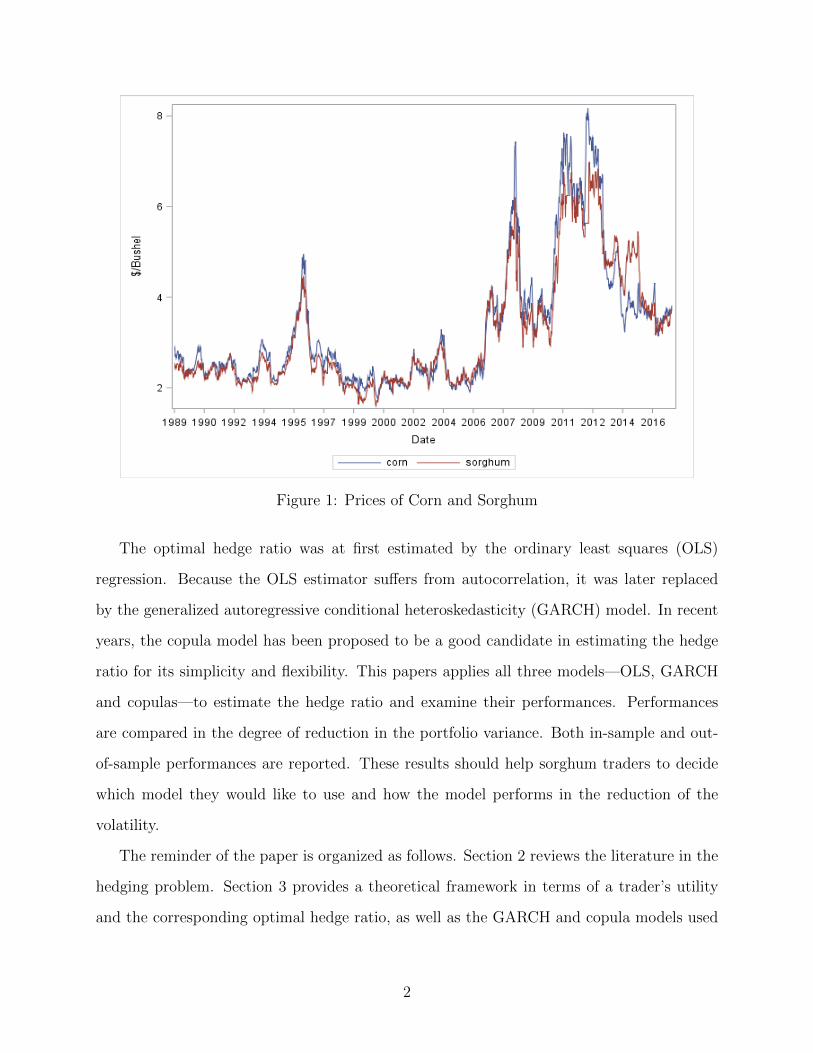
Figure 1: Prices of Corn and Sorghum

The optimal hedge ratio was at first estimated by the ordinary least squares (OLS)

regression. Because the OLS estimator suffers from autocorrelation, it was later replaced

by the generalized autoregressive conditional heteroskedasticity (GARCH) model. In recent

years, the copula model has been proposed to be a good candidate in estimating the hedge

ratio for its simplicity and flexibility. This papers applies all three models—OLS, GARCH

and copulas—to estimate the hedge ratio and examine their performances. Performances

are compared in the degree of reduction in the portfolio variance. Both in-sample and out-

of-sample performances are reported. These results should help sorghum traders to decide

which model they would like to use and how the model performs in the reduction of the

volatility.

The reminder of the paper is organized as follows. Section 2 reviews the literature in the

hedging problem. Section 3 provides a theoretical framework in terms of a trader’s utility

and the corresponding optimal hedge ratio, as well as the GARCH and copula models used

2

to estimate the ratio. Section 4 presents empirical results for the estimation and hedging

performance. Section 5 summarizes the results and the implications of the paper.

2 Literature Review

2.1 Conventional Hedge Ratio Estimation

The optimal hedge ratio was first estimated by an OLS or GLS regression on the price level or

percentage change. In the literature of the agriculture industry, Hayenga and Pietre (1982)

used live hog futures to hedge pork prices for wholesale pork producers. Brown and Stewart

(1985) used the price difference to decide the hedge ratio in the wheat, corn and soybean

markets. Harvey, Ted and Marvin (1986) estimated the optimal hedge ratios using both

price differences and price levels in a cross-hedge and showed that the two optimal hedge

ratios are significantly different. They argued that regression parameters should be judged

by the objective utility function.

2.2 Estimation by A GARCH Model

Ordinary price regression suffers from the fact the OLS residuals are often serially correlated.

More importantly, the OLS regression implicitly assumes a constant relationship between

the spot and the futures prices, which ignores the maturity effect and the change in market

conditions (Herbst et al., 1993).2 To allow for time-varying volatility, Engle (1982) proposed

the autoregressive conditional heteroscedasticity (ARCH) model to allow the variance to

depend on previous deviations. A more generalized ARCH (GARCH) was proposed by

Bollerslev (1986) that allowed the variance to change over the previous estimated variance.

Since then, much hedge ratio research has been done using a GARCH model (Baillie and

Robert 1991; Myers and Robert 1992).

2The maturity effect implies that the spot and the futures prices converge at maturity and that the pricevolatility of a futures contract increases as it approaches maturity.

3

The univariate GARCH model works well for a single price, but to estimate the optimal

hedge ratio between two prices, multivariate models were proposed by Engle and Kroner

(1995) to allow the variance and covariance to change over time. In terms of the bivari-

ate GARCH model, Bollerslev (1990) proposed a constant conditional correlation (CCC)

GARCH to estimate the correlation of spot and futures prices. Engle and Sheppard (2001)

extended the CCC GARCH to the dynamic conditional correlation (DCG) GARCH to allow

the correlation to vary over time. The more complicated model is the BEKK model (Baba,

Engle, Kraft and Kroner, 1990), which ensures that the variance covariance matrix is positive

definite.

Bera, Garcia, and Roh (1997) applied the CCC GARCH, Diagonal VECH GARCH , and

BEKK to estimate the optimal hedge ratio in the corn and soybeans markets.3 Their results

suggest that the Diagonal VECH GARCH model has the greatest performance, followed

by the OLS estimation and the CCC GARCH model. The BEKK model works as well as

the CCC GARCH model in the in-sample comparison, but much worse in the out-of-sample

comparison.

2.3 Estimation by A Copula Model

In a multivariate GARCH model, the distribution is often assumed to be joint normal or

student’s t, both of which have symmetric tail dependence. If the distribution assumption

does not hold, then the model cannot be accurately applied. One way to allow for a more

flexible joint distribution is to use a copula model. A copula model does not have any

assumption on the marginal distributions. This makes the copula a good candidate to

capture nonlinear dependency with different marginal distributions. Also, the copula model

is able to estimate both symmetric and asymmetric tail dependencies.

3The Diagonal VECH GARCH is a restricted version of the multivariate GARCH where the conditionalvariance (h11,t and h22,t) and covariance (h12,t) in the variance covariance matrix Ht only depend on its ownlagged squared residuals and lagged conditional variance. More specifically, the conditional variance h11,tonly depends on h11,t−1 and ε21,t−1; the conditional variance h22,t only depends on h22,t−1 and ε22,t−1; andthe covariance h12,t only depends on h12,t−1 ε1,t−1ε2,t−1.

4

Patton (2006) introduced a dynamic copula model that linked the GARCH model and a

copula model. The model estimates the marginal distribution by the GARCH model for each

price, then applies a copula model to estimate the correlation between the two prices. He used

the model to estimate the relationship between different countries’ exchange rates and showed

that a structural change emerged between the US dollar and the Japanese yen after the

Euro was issued. Rodriguez (2007) applied a dynamic copula model with Markov switching

parameters to identify the tail dependence during the financial crisis caused by a contagion

phenomenon. Wu, Chung and Chang (2010) investigated the correlation between oil price

and the exchange rate and demonstrated that a copula-based GARCH model exhibits greater

economics benefit of an investor than an OLS and other multivariate GARCH models.

The dynamic copula model has recently been applied in the study of the hedge ratio.

Hsu, Tseng and Wang (2008) estimated the hedge ratio by the dynamic Normal, Gumbel

and Clayton copula models. They showed that estimates from these copula models have

better performance in the reduction of the portfolio variance than the conventional OLS or

GARCH models.

In agriculture, Power, Vedenov, Anderson and Klose (2013) proposed a nonparametric

copula-based GARCH model to estimate the hedge ratio between cash and futures prices

for corn and cattle. They showed that the application of the copula has better performance

in terms of tail risk (expected shortfall), but worse in terms of variance reduction than the

BEKK model. Zhao and Goodwin (2012) used a dynamic copula model to calculate the

hedge ratio of using corn to cross-hedge grain sorghum and wheat to cross-hedge barley.

However they did not report the performance of the hedging strategy.

This paper applies methodology similar to that introduced by Zhao and Goodwin (2012)

with more detailed analysis of price relationship and hedge effectiveness. Both constant

and dynamic copula models are applied to determine the optimal hedge ratio, and hedging

performance is compared, both in-sample and out-of sample.

5

3 Model

3.1 The Utility Model in the Hedging Problem

For a sorghum trader who wants to hedge the price risk of grain sorghum, he or she can

take an opposite position in the corn futures market. The philosophy behind this is to offset

losses (gains) in the sorghum market by the gains (losses) from the corn futures market.

The return from a hedging activity depends on the change of sorghum cash prices and

corn futures prices from time t− 1 to t, and the hedge ratio. Let ∆st = st− st−1 denote the

change of sorghum cash prices and ∆ft = ft− ft−1 denote the change of corn futures prices;

for each unit of sorghum, if h units of corn is hedged in the futures market, the hedging

return xt on the portfolio is calculated to be:

xt = ∆st + h∆ft (1)

The objective of a hedging strategy is to maximize a trader’s utility given that this

trader is risk-averse. Therefore, the optimal hedge units, or the optimal hedge ratio h should

depend on a trader’s utility function. One of the most popular utility functions in the hedging

literature is the mean-variance utility function proposed by Kahl (1983). It derives from the

expectation of a concave exponentiation utility function. The mean-variance utility function

is defined as:

U(x) = E(x)− λ

2· V ar(x) (2)

where λ is Arrow-Pratt measure of absolute risk-aversion. More details on the mean-variance

utility function can be found in Appendix A.1.

Suppose both prices follow a martingale distribution in which the expectation of the price

in the next period equals the present price.4 The expectation and variance of the return on

4The martingale distribution assumes that the expected value of a random variable equals the presentedobserved value given all the prior information.

6

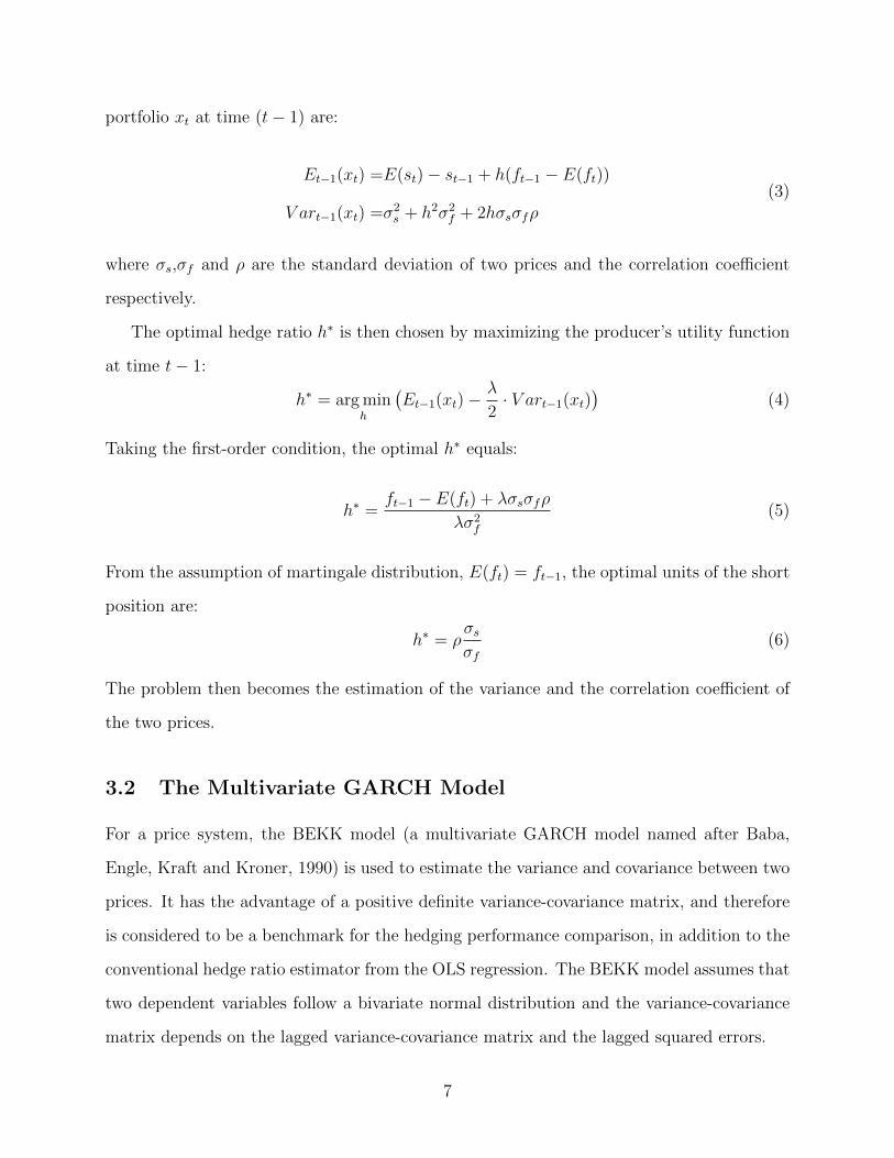
portfolio xt at time (t− 1) are:

Et−1(xt) =E(st)− st−1 + h(ft−1 − E(ft))

V art−1(xt) =σ2s + h2σ2

f + 2hσsσfρ(3)

where σs,σf and ρ are the standard deviation of two prices and the correlation coefficient

respectively.

The optimal hedge ratio h∗ is then chosen by maximizing the producer’s utility function

at time t− 1:

h∗ = arg minh

(Et−1(xt)−

λ

2· V art−1(xt)

)(4)

Taking the first-order condition, the optimal h∗ equals:

h∗ =ft−1 − E(ft) + λσsσfρ

λσ2f

(5)

From the assumption of martingale distribution, E(ft) = ft−1, the optimal units of the short

position are:

h∗ = ρσsσf

(6)

The problem then becomes the estimation of the variance and the correlation coefficient of

the two prices.

3.2 The Multivariate GARCH Model

For a price system, the BEKK model (a multivariate GARCH model named after Baba,

Engle, Kraft and Kroner, 1990) is used to estimate the variance and covariance between two

prices. It has the advantage of a positive definite variance-covariance matrix, and therefore

is considered to be a benchmark for the hedging performance comparison, in addition to the

conventional hedge ratio estimator from the OLS regression. The BEKK model assumes that

two dependent variables follow a bivariate normal distribution and the variance-covariance

matrix depends on the lagged variance-covariance matrix and the lagged squared errors.

7

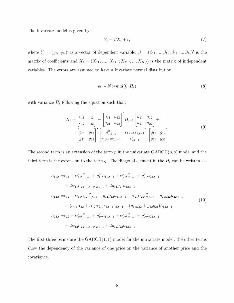
The bivariate model is given by:

Yt = βXt + εt (7)

where Yt = (y1t, y2t)′ is a vector of dependent variable, β = (β11, ..., β1k; β21, ..., β2k)

′ is the

matrix of coefficients and Xt = (X11,t, ..., X1k,t;X21,t, ..., X2k,t) is the matrix of independent

variables. The errors are assumed to have a bivariate normal distribution

εt ∼ Normal(0, Ht) (8)

with variance Ht following the equation such that:

Ht =

[c11 c12

c12 c22

]+

[a11 a12

a21 a22

]′Ht−1

[a11 a12

a21 a22

]+[

g11 g12

g21 g22

]′ [ε21,t−1 ε1,t−1ε2,t−1

ε1,t−1ε2,t−1 ε22,t−1

][g11 g12

g21 g22

] (9)

The second term is an extension of the term p in the univariate GARCH(p, q) model and the

third term is the extension to the term q. The diagonal element in the Ht can be written as:

h11,t =c11 + α211ε

21,t−1 + g2

11h11,t−1 + α221ε

22,t−1 + g2

21h22,t−1

+ 2α11α21ε1,t−1ε2,t−1 + 2g11g21h12,t−1

h12,t =c12 + α11α12ε21,t−1 + g11g12h11,t−1 + α21α22ε

22,t−1 + g21g22h22,t−1

+ (α11α22 + α12α21)ε1,t−1ε2,t−1 + (g11g22 + g12g21)h12,t−1

h22,t =c22 + α212ε

21,t−1 + g2

12h11,t−1 + α222ε

22,t−1 + g2

22h22,t−1

+ 2α12α22ε1,t−1ε2,t−1 + 2g12g22h12,t−1

(10)

The first three terms are the GARCH(1, 1) model for the univariate model; the other terms

show the dependency of the variance of one price on the variance of another price and the

covariance.

8

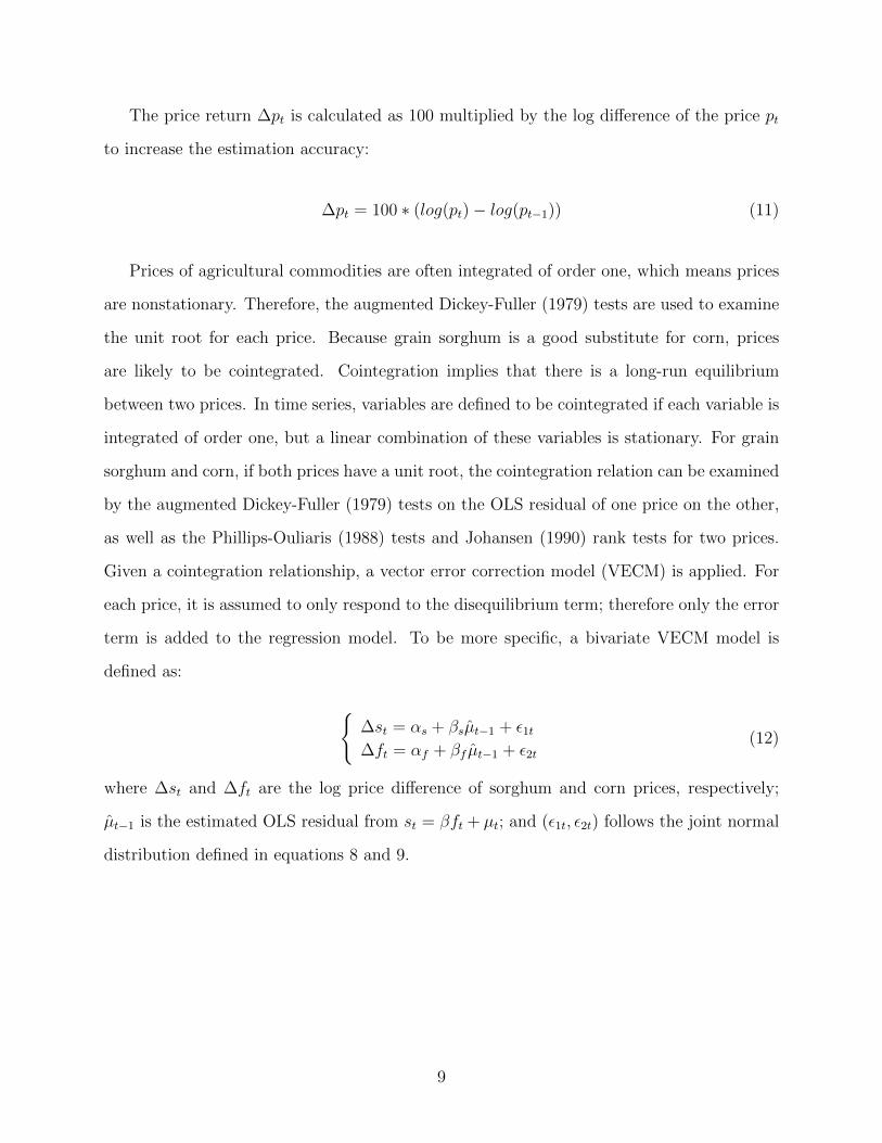
The price return ∆pt is calculated as 100 multiplied by the log difference of the price pt

to increase the estimation accuracy:

∆pt = 100 ∗ (log(pt)− log(pt−1)) (11)

Prices of agricultural commodities are often integrated of order one, which means prices

are nonstationary. Therefore, the augmented Dickey-Fuller (1979) tests are used to examine

the unit root for each price. Because grain sorghum is a good substitute for corn, prices

are likely to be cointegrated. Cointegration implies that there is a long-run equilibrium

between two prices. In time series, variables are defined to be cointegrated if each variable is

integrated of order one, but a linear combination of these variables is stationary. For grain

sorghum and corn, if both prices have a unit root, the cointegration relation can be examined

by the augmented Dickey-Fuller (1979) tests on the OLS residual of one price on the other,

as well as the Phillips-Ouliaris (1988) tests and Johansen (1990) rank tests for two prices.

Given a cointegration relationship, a vector error correction model (VECM) is applied. For

each price, it is assumed to only respond to the disequilibrium term; therefore only the error

term is added to the regression model. To be more specific, a bivariate VECM model is

defined as:

{∆st = αs + βsµt−1 + ε1t∆ft = αf + βf µt−1 + ε2t

(12)

where ∆st and ∆ft are the log price difference of sorghum and corn prices, respectively;

µt−1 is the estimated OLS residual from st = βft + µt; and (ε1t, ε2t) follows the joint normal

distribution defined in equations 8 and 9.

9

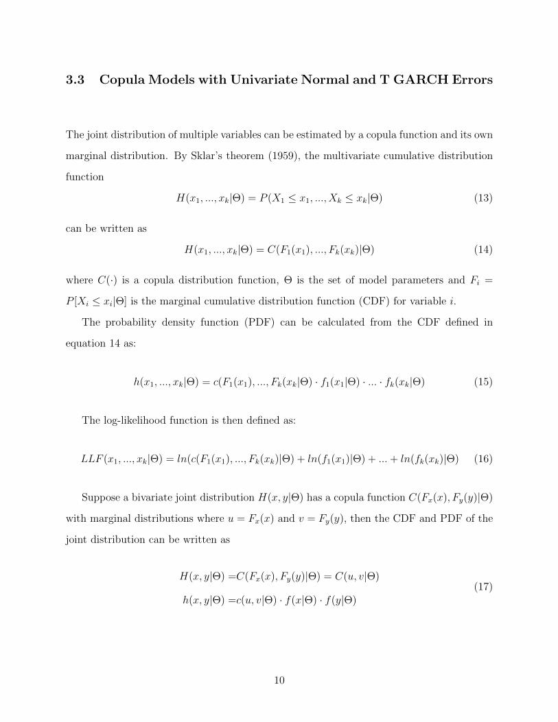
3.3 Copula Models with Univariate Normal and T GARCH Errors

The joint distribution of multiple variables can be estimated by a copula function and its own

marginal distribution. By Sklar’s theorem (1959), the multivariate cumulative distribution

function

H(x1, ..., xk|Θ) = P (X1 ≤ x1, ..., Xk ≤ xk|Θ) (13)

can be written as

H(x1, ..., xk|Θ) = C(F1(x1), ..., Fk(xk)|Θ) (14)

where C(·) is a copula distribution function, Θ is the set of model parameters and Fi =

P [Xi ≤ xi|Θ] is the marginal cumulative distribution function (CDF) for variable i.

The probability density function (PDF) can be calculated from the CDF defined in

equation 14 as:

h(x1, ..., xk|Θ) = c(F1(x1), ..., Fk(xk|Θ) · f1(x1|Θ) · ... · fk(xk|Θ) (15)

The log-likelihood function is then defined as:

LLF (x1, ..., xk|Θ) = ln(c(F1(x1), ..., Fk(xk)|Θ) + ln(f1(x1)|Θ) + ...+ ln(fk(xk)|Θ) (16)

Suppose a bivariate joint distribution H(x, y|Θ) has a copula function C(Fx(x), Fy(y)|Θ)

with marginal distributions where u = Fx(x) and v = Fy(y), then the CDF and PDF of the

joint distribution can be written as

H(x, y|Θ) =C(Fx(x), Fy(y)|Θ) = C(u, v|Θ)

h(x, y|Θ) =c(u, v|Θ) · f(x|Θ) · f(y|Θ)(17)

10

and its log-likelihood function is

LLF (x, y|Θ) = ln(c(u, v)|Θ) + ln(f(x)|Θ) + ln(f(y)|Θ) (18)

The likelihood function is usually maximized in two steps to simplify calculation under the

full likelihood function. The first step is to estimate the marginal distribution by maximizing

ln(f(x)|Θx) and ln(f(y)|Θy) separately. The second step is to estimate the copula function

by maximizing the likelihood function ln(c(u, v)|Θx, Θy,Θc) given the estimates Θx and Θy

in the first step. As Patton (2006) noted, the estimates are consistent and asymptotically

normal under standard conditions.

If prices are conitegrated, the marginal distribution of each price can be estimated by a

univariate error correction model with a GARCH error term. A univariate error correction

model is defined as:

∆yt = α + βµt−1 + εt (19)

where µt−1 is the estimated OLS residual and the error term εt follows a normal or t distri-

bution with mean 0 and variance ht. The variance term ht in a GARCH (p, q) model follows

the equation:

ht = c+

q∑i=1

αiε2t−i +

p∑j=1

γjht−j (20)

In the second step, the two estimated error terms ε1t and ε2t are transformed to ut and

vt by the inverse normal or t CDF. Copula coefficients are then estimated by the copula

likelihood function.

The candidate bivariate copula models include a normal, Student’s t, and three Archimedean

families of copulas—Clayton, Frank and Gumbel. Among these copulas, normal, student’s

t and Frank copula have symmetric tail dependence, and the Clayton and Gumbel copulas

have asymmetric tail dependence. Tail dependence should affect the linear correlation of two

prices under extreme conditions, but is not studied because this paper focuses more on the

11

hedging activity at all times rather than a specific period of time. Because the joint distribu-

tion depends on both the copula and marginal distributions, different correlation coefficients

can be estimated by selecting either a different copula or different marginal distributions.

Therefore, models with different copulas and marginal distributions are examined in the pa-

per and the main purpose is to find the model that can best describe the linear correlation

between two or more prices and apply it in the daily hedging activity. The CDF and PDF

of all copula models are summarized in Table ??.

3.4 Time-Varying Copula Model

It is possible that parameters in copulas change from time. Therefore, two dynamic copula

models defined by Patton (2006) are considered to capture the variation of parameters by

time. The first is the Gaussian copula with symmetric tail dependence, and the other is the

Gumbel Copula with the asymmetric tail dependence.

In the GARCH model, the variance is allowed to depend on the lagged estimated variance

and the lagged squared errors. Similarly, the copula coefficient ρ in the Gaussian copula and

θ in the Gumbel copula are set to depend on its lagged value and the lagged conditional

covariance.

The coefficient in the dynamic Gaussian copula is defined as:

ρt = z

(wρ + βρρt−1 + α

1

q

q∑j=1

F−1u (ut−j) · F−1

v (vt−j)

)(21)

where F−1u (·) and F−1

v (·) are the inverse CDF of the marginal distribution of u and v, and

z(x) ≡ (1− e−x)(1 + e−x)−1 = tanh(x/2) is the function that keeps ρ in the range of (−1, 1).

For the dynamic Gumbel copula, the coefficient θ equals:

θt = k

(wθ + βθθt−1 + α

1

q

q∑j=1

F−1u (ut−j) · F−1

v (vt−j)

)(22)

where k(x) ≡ 1 + x2 to keep the variable θ in the range of [1,∞)

12

Here, only the first lag of the coefficient is considered, so the model is similar to the

multivariate GARCH model with p = 1 and q = 1. This should make the comparison more

robust as the assumption of the lag dependency is same for different models.

4 Empirical Results

Corn prices are measured as the nearby futures from the Chicago Board of Trade (CBOT),

and sorghum cash prices are measured from Gulf Coast. The data are obtained from the

Commodity Research Bureau (CRB). Weekly prices from January 1989 to June 2017 are

used, as daily cash prices often show little or no change. The summary statistics are presented

in Table 2. For each price, the mean of price difference is close to zero and the standard

error is significantly large compared to the mean, which shows high volatility in the price

itself.

4.1 Results from Cointegration Tests and the BEKK GARCH

Model

The ADF tests are applied to each price to check the existence of the unit root. The lag is

selected to be one week or one month (4 weeks). The large p-values in table 3 indicate that

we fail to reject the null of a unit root, which means that prices are nonstationary.

Therefore, cointegration test are applied and results are summarized in Table 4. Strong

cointegration relations are observed between corn and grain sorghum, since all six tests reject

the null hypothesis of no cointegration. This implies that there is a long run equilibrium

between corn and sorghum prices.

Due to the cointegration relationship, the BEKK model is estimated based on the vector

error correction model defined in equation 12, with the variance-covariance matrix defined

in equation 9. Results are presented in Table 5.

In theory, adjustment coefficients for the sorghum price should be negative to eliminate

the disequilibrium caused by corn prices, but the estimate is a positive number, though not

13

statistically significant. This may imply that the return on the sorghum price is unpre-

dictable. For corn futures prices, the adjustment coefficient is large and significant, which

indicates that the nearest futures price of corn may depend on the disequilibrium between

the sorghum spot price and corn price.

Results from the BEKK model indicate that the variance of each price mostly de-

pends on the lag variance of two prices rather than the lag covariance, as the coefficients

α12, α21, g12, g21 are relatively small compared to coefficients α11, α22, g11, g22. The estimated

variance of each price is presented in Figure 2. In the figure, several price volatilities hikes

are observed. The first is the 2008-2009 period. In this period, prices of agricultural com-

modities spiked in early 2008 due to the food crisis and later decreased dramatically due to

the financial crisis.5 The second hikes is observed for the sorghum in September. This hike is

caused by the data. Prices changes for sorghum were zero from June to September in 2012,

and these changes accumulated and finally occurred in September, which leads to a large

volatility. The last is between the mid-2013, when corn prices were decreased by the high

production forecast and the proposal of a reduction in biofuel mandate by the Environmental

Protection Agency.

It is complicated to calculate the single effect of each variable, such as lagged variance

or covariance, on the conditional covariance term; therefore, the correlation coefficient from

the BEKK model is presented in Figure 2.

The correlation coefficient is stable most of the time, as it moves up and down from the

average correlation coefficient of 0.81. In July 1996, the corn price took a huge fall. The

price was decreased by 16% in one week and that probably caused a negative correlation.

The low correlation coefficients in July 2011 and July 2012 are caused by zero changes in

the sorghum prices in the data. Because sorghum prices changes kept zero for several weeks,

the model assumes that corn prices were not related to sorghum prices in these periods.

The low correlation coefficient in July 2013 is caused by other factors, as data do show price

5According to the International Food Policy Research Institute, the major causes of the 2007-2008 foodcrisis include “...rising energy prices, the depreciation of the U.S. dollar, low interest rates, and investmentportfolio adjustments in favor of commodities” (Headey and Fan, 2010).

14

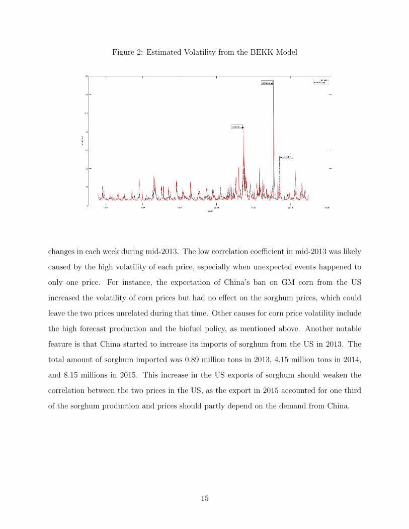
Figure 2: Estimated Volatility from the BEKK Model

changes in each week during mid-2013. The low correlation coefficient in mid-2013 was likely

caused by the high volatility of each price, especially when unexpected events happened to

only one price. For instance, the expectation of China’s ban on GM corn from the US

increased the volatility of corn prices but had no effect on the sorghum prices, which could

leave the two prices unrelated during that time. Other causes for corn price volatility include

the high forecast production and the biofuel policy, as mentioned above. Another notable

feature is that China started to increase its imports of sorghum from the US in 2013. The

total amount of sorghum imported was 0.89 million tons in 2013, 4.15 million tons in 2014,

and 8.15 millions in 2015. This increase in the US exports of sorghum should weaken the

correlation between the two prices in the US, as the export in 2015 accounted for one third

of the sorghum production and prices should partly depend on the demand from China.

15

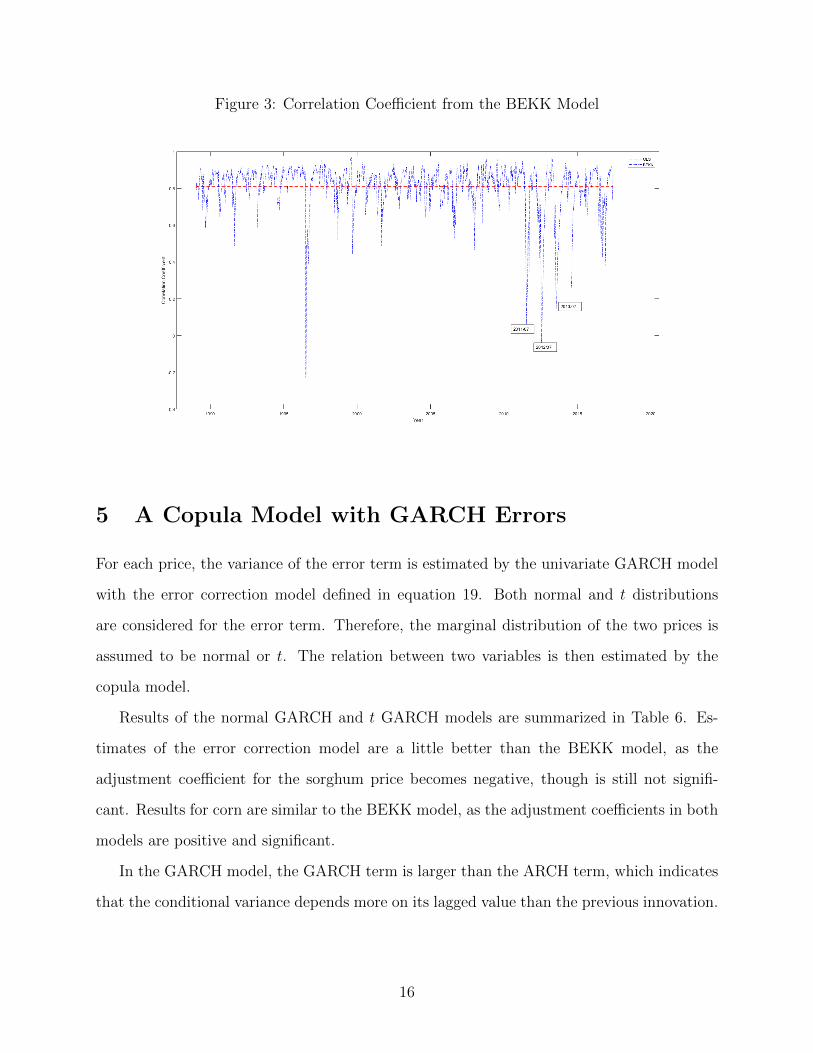
Figure 3: Correlation Coefficient from the BEKK Model

5 A Copula Model with GARCH Errors

For each price, the variance of the error term is estimated by the univariate GARCH model

with the error correction model defined in equation 19. Both normal and t distributions

are considered for the error term. Therefore, the marginal distribution of the two prices is

assumed to be normal or t. The relation between two variables is then estimated by the

copula model.

Results of the normal GARCH and t GARCH models are summarized in Table 6. Es-

timates of the error correction model are a little better than the BEKK model, as the

adjustment coefficient for the sorghum price becomes negative, though is still not signifi-

cant. Results for corn are similar to the BEKK model, as the adjustment coefficients in both

models are positive and significant.

In the GARCH model, the GARCH term is larger than the ARCH term, which indicates

that the conditional variance depends more on its lagged value than the previous innovation.

16

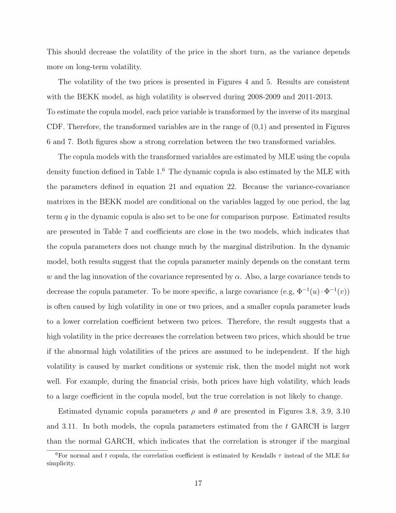
This should decrease the volatility of the price in the short turn, as the variance depends

more on long-term volatility.

The volatility of the two prices is presented in Figures 4 and 5. Results are consistent

with the BEKK model, as high volatility is observed during 2008-2009 and 2011-2013.

To estimate the copula model, each price variable is transformed by the inverse of its marginal

CDF. Therefore, the transformed variables are in the range of (0,1) and presented in Figures

6 and 7. Both figures show a strong correlation between the two transformed variables.

The copula models with the transformed variables are estimated by MLE using the copula

density function defined in Table 1.6 The dynamic copula is also estimated by the MLE with

the parameters defined in equation 21 and equation 22. Because the variance-covariance

matrixes in the BEKK model are conditional on the variables lagged by one period, the lag

term q in the dynamic copula is also set to be one for comparison purpose. Estimated results

are presented in Table 7 and coefficients are close in the two models, which indicates that

the copula parameters does not change much by the marginal distribution. In the dynamic

model, both results suggest that the copula parameter mainly depends on the constant term

w and the lag innovation of the covariance represented by α. Also, a large covariance tends to

decrease the copula parameter. To be more specific, a large covariance (e.g, Φ−1(u) ·Φ−1(v))

is often caused by high volatility in one or two prices, and a smaller copula parameter leads

to a lower correlation coefficient between two prices. Therefore, the result suggests that a

high volatility in the price decreases the correlation between two prices, which should be true

if the abnormal high volatilities of the prices are assumed to be independent. If the high

volatility is caused by market conditions or systemic risk, then the model might not work

well. For example, during the financial crisis, both prices have high volatility, which leads

to a large coefficient in the copula model, but the true correlation is not likely to change.

Estimated dynamic copula parameters ρ and θ are presented in Figures 3.8, 3.9, 3.10

and 3.11. In both models, the copula parameters estimated from the t GARCH is larger

than the normal GARCH, which indicates that the correlation is stronger if the marginal

6For normal and t copula, the correlation coefficient is estimated by Kendalls τ instead of the MLE forsimplicity.

17

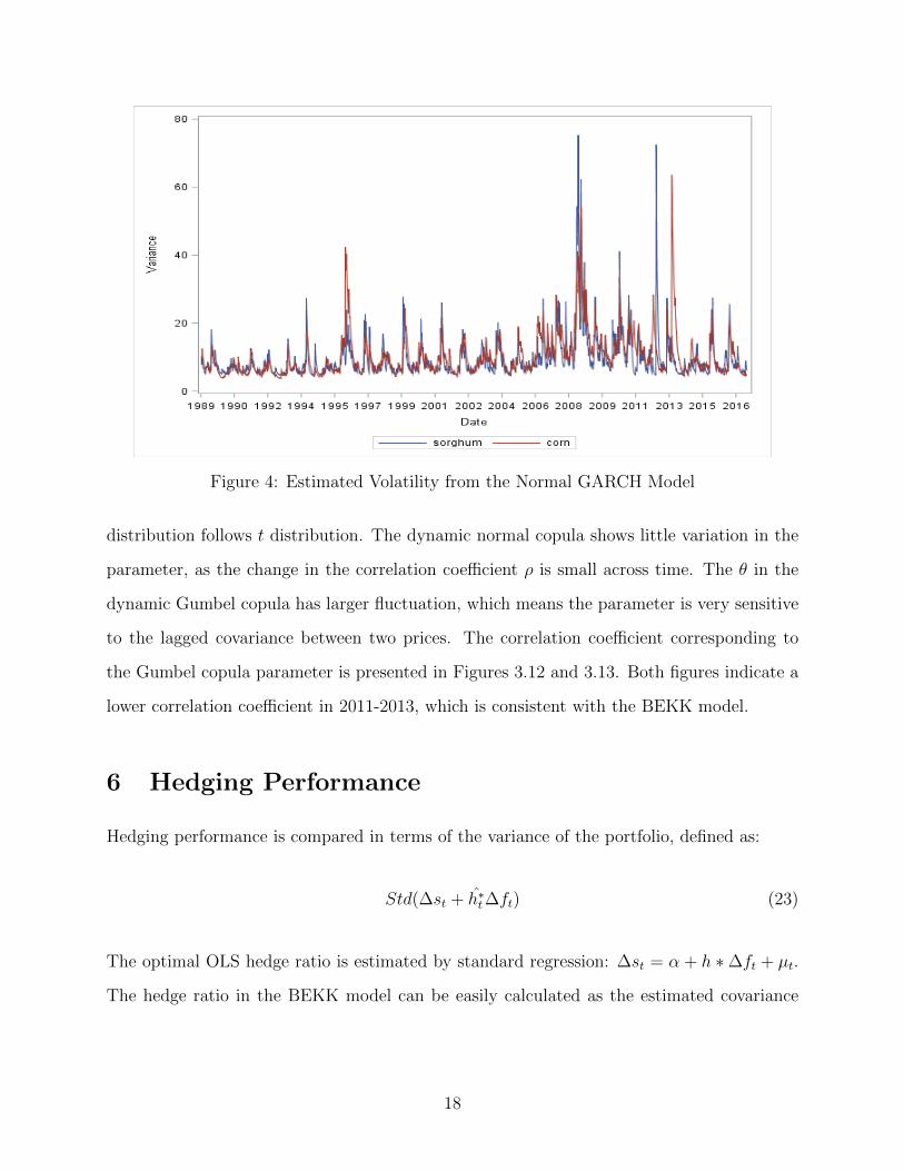
Figure 4: Estimated Volatility from the Normal GARCH Model

distribution follows t distribution. The dynamic normal copula shows little variation in the

parameter, as the change in the correlation coefficient ρ is small across time. The θ in the

dynamic Gumbel copula has larger fluctuation, which means the parameter is very sensitive

to the lagged covariance between two prices. The correlation coefficient corresponding to

the Gumbel copula parameter is presented in Figures 3.12 and 3.13. Both figures indicate a

lower correlation coefficient in 2011-2013, which is consistent with the BEKK model.

6 Hedging Performance

Hedging performance is compared in terms of the variance of the portfolio, defined as:

Std(∆st + h∗t∆ft) (23)

The optimal OLS hedge ratio is estimated by standard regression: ∆st = α + h ∗∆ft + µt.

The hedge ratio in the BEKK model can be easily calculated as the estimated covariance

18

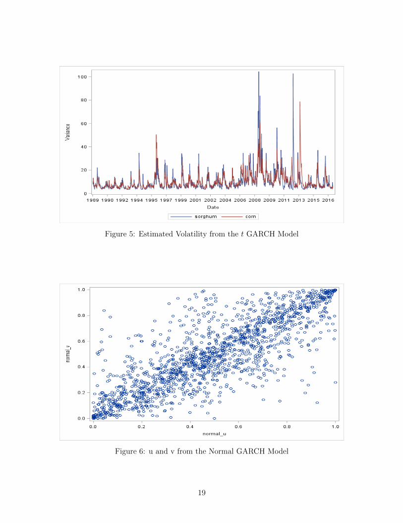
Figure 5: Estimated Volatility from the t GARCH Model

Figure 6: u and v from the Normal GARCH Model

19

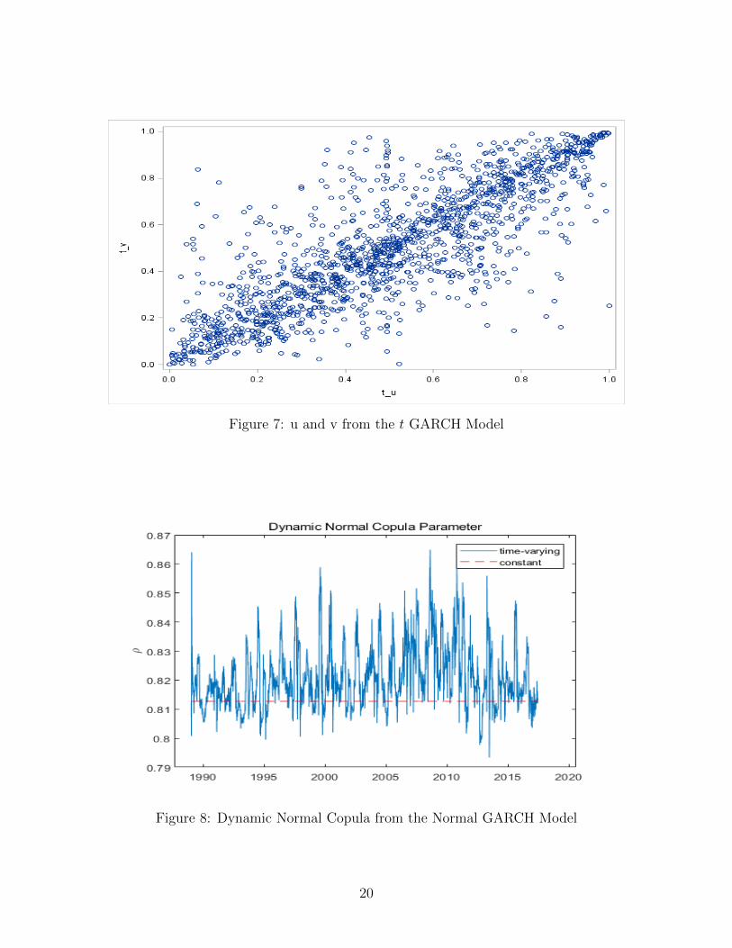
Figure 7: u and v from the t GARCH Model

Figure 8: Dynamic Normal Copula from the Normal GARCH Model

20

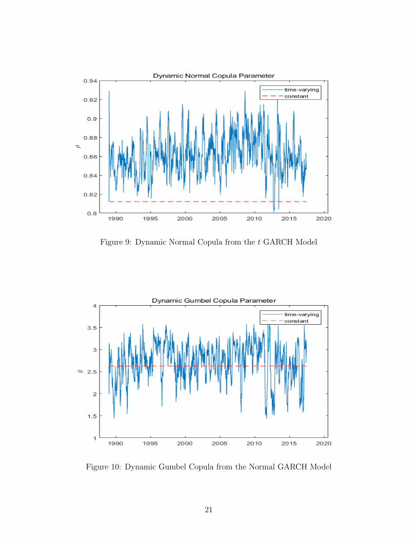
Figure 9: Dynamic Normal Copula from the t GARCH Model

Figure 10: Dynamic Gumbel Copula from the Normal GARCH Model

21

Figure 11: Dynamic Gumbel Copula from t GARCH Model

Figure 12: Dynamic Gumbel Copula from the Normal GARCH Model

22

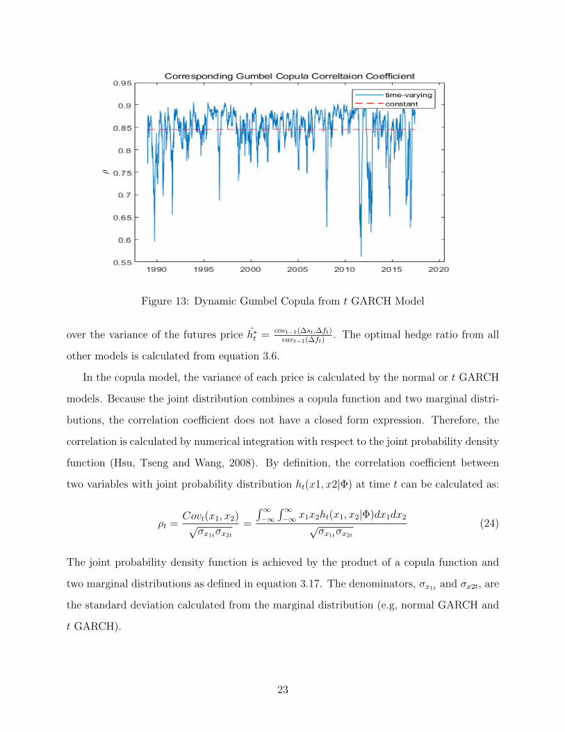
Figure 13: Dynamic Gumbel Copula from t GARCH Model

over the variance of the futures price h∗t = covt−1(∆st,∆ft)vart−1(∆ft)

. The optimal hedge ratio from all

other models is calculated from equation 3.6.

In the copula model, the variance of each price is calculated by the normal or t GARCH

models. Because the joint distribution combines a copula function and two marginal distri-

butions, the correlation coefficient does not have a closed form expression. Therefore, the

correlation is calculated by numerical integration with respect to the joint probability density

function (Hsu, Tseng and Wang, 2008). By definition, the correlation coefficient between

two variables with joint probability distribution ht(x1, x2|Φ) at time t can be calculated as:

ρt =Covt(x1, x2)√σx1tσx2t

=

∫∞−∞

∫∞−∞ x1x2ht(x1, x2|Φ)dx1dx2

√σx1tσx2t

(24)

The joint probability density function is achieved by the product of a copula function and

two marginal distributions as defined in equation 3.17. The denominators, σx1t and σx2t, are

the standard deviation calculated from the marginal distribution (e.g, normal GARCH and

t GARCH).

23

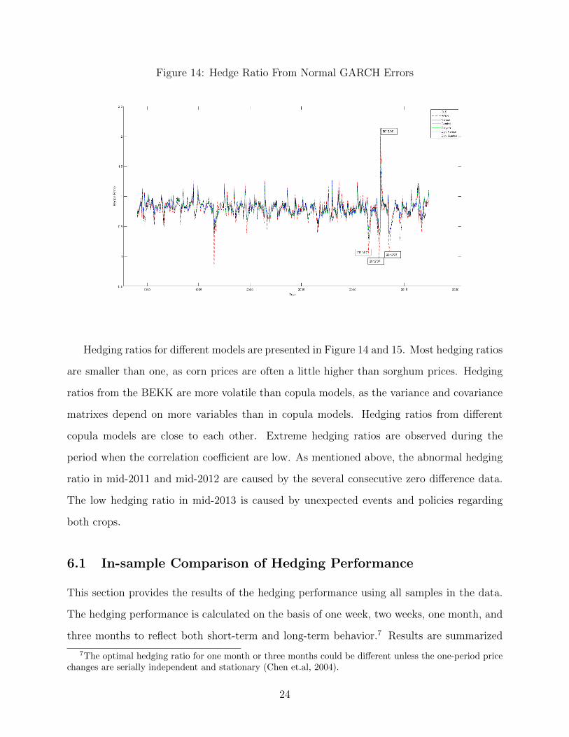
Figure 14: Hedge Ratio From Normal GARCH Errors

Hedging ratios for different models are presented in Figure 14 and 15. Most hedging ratios

are smaller than one, as corn prices are often a little higher than sorghum prices. Hedging

ratios from the BEKK are more volatile than copula models, as the variance and covariance

matrixes depend on more variables than in copula models. Hedging ratios from different

copula models are close to each other. Extreme hedging ratios are observed during the

period when the correlation coefficient are low. As mentioned above, the abnormal hedging

ratio in mid-2011 and mid-2012 are caused by the several consecutive zero difference data.

The low hedging ratio in mid-2013 is caused by unexpected events and policies regarding

both crops.

6.1 In-sample Comparison of Hedging Performance

This section provides the results of the hedging performance using all samples in the data.

The hedging performance is calculated on the basis of one week, two weeks, one month, and

three months to reflect both short-term and long-term behavior.7 Results are summarized

7The optimal hedging ratio for one month or three months could be different unless the one-period pricechanges are serially independent and stationary (Chen et.al, 2004).

24

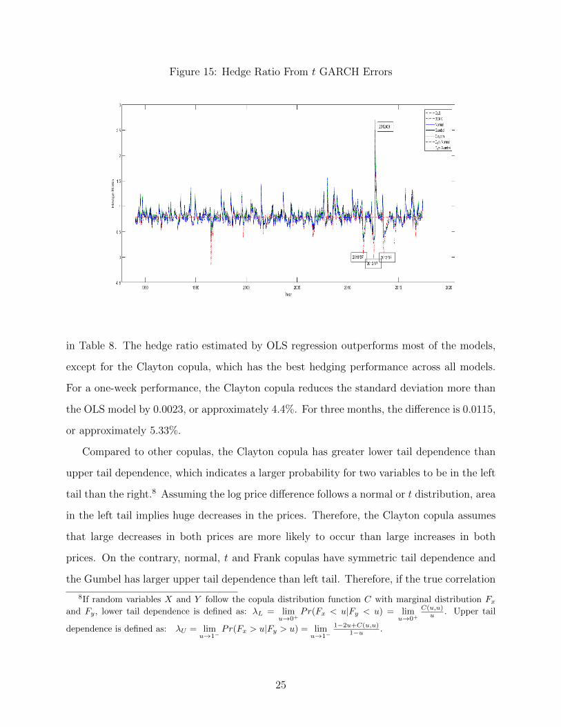
Figure 15: Hedge Ratio From t GARCH Errors

in Table 8. The hedge ratio estimated by OLS regression outperforms most of the models,

except for the Clayton copula, which has the best hedging performance across all models.

For a one-week performance, the Clayton copula reduces the standard deviation more than

the OLS model by 0.0023, or approximately 4.4%. For three months, the difference is 0.0115,

or approximately 5.33%.

Compared to other copulas, the Clayton copula has greater lower tail dependence than

upper tail dependence, which indicates a larger probability for two variables to be in the left

tail than the right.8 Assuming the log price difference follows a normal or t distribution, area

in the left tail implies huge decreases in the prices. Therefore, the Clayton copula assumes

that large decreases in both prices are more likely to occur than large increases in both

prices. On the contrary, normal, t and Frank copulas have symmetric tail dependence and

the Gumbel has larger upper tail dependence than left tail. Therefore, if the true correlation

8If random variables X and Y follow the copula distribution function C with marginal distribution Fx

and Fy, lower tail dependence is defined as: λL = limu→0+

Pr(Fx < u|Fy < u) = limu→0+

C(u,u)u . Upper tail

dependence is defined as: λU = limu→1−

Pr(Fx > u|Fy > u) = limu→1−

1−2u+C(u,u)1−u .

25

has the characteristic that decreases in prices are more related to each other than increases,

the Clayton copula is likely to capture this characteristic and present better results.

It is surprising to observe that dynamic copula models often perform worse than the

nondynamic ones. One possible explanation is that the dynamic model does not capture the

true correlation when there is a systemic risk, or the true correlation is more stable and the

estimated correlation coefficient is too sensitive to the price volatility.

6.2 Out-of-sample Comparison of Hedging Performance

In-sample models are often criticized for the overfitting issue, especially in the forecast area,

and a model with good in-sample performance does not necessarily demonstrate good out-

of-sample performance.

Therefore, an out-of-sample comparison is conducted in this section. The out-of-sample

comparison removes the last 100 observations from the data, or approximately two years.

For each observation being removed, the hedge ratio is estimated using all previous data.

This method ensures that each out-of-sample estimation uses all of the available information.

More specifically, data from 07/15/2015 to 06/06/2017 are first taken out from the whole

dataset. The hedge ratio for 07/15/2015 is estimated using all the data before it (from

01/01/1989 to 07/08/2015). For the next observation on 07/22/2015, the estimation adds

the data for 07/15/2015 to the model. By continuously updating the dataset in the model,

100, 99, 97 and 89 hedging outcomes are computed for one week, two weeks, one month, and

three months.

Standard deviations of the return on these out-of-sample data are presented in Table

9. The out-of-sample comparison still favors the Clayton copula, as it shows the minimum

standard deviation of all the models. Unlike in the in-sample comparison, the OLS hedging

estimator is worse than most of the models. The second-best hedging estimator is the

BEKK model, which is also considered to be a benchmark in the comparison. Compared

to the BEKK model, the Clayton copula reduced the standard deviation more by 0.001, or

approximately 2.30%, in one week of hedging and 0.0018, or approximately 1.61%, in three

26

months of hedging. The performance of the dynamic copula model is still worse or equal to

the nondynamic copula model, which suggests that it does not capture the correlation well

across time.

7 Conclusion

Grain Sorghum is an important animal feed in the livestock industry and considered to be

good substitute for corn. Because there is no futures market for grain sorghum, it is a good

option for sorghum traders to hedge the price risk by corn futures, as two prices are highly

related. The most important question in this hedging problem is to find the optimal hedge

ratio for the traders.

The optimal hedge ratio derives from the popular mean-variance utility function and is

decided by the variance and correlation coefficient between grain sorghum spot prices and

corn futures prices. The traditional estimation methods include the OLS and multivariate

GARCH models, where the joint distribution is often assumed to be normal. This paper

applies a copula model to estimate the variance and correlation coefficient between two

prices. Application of a copula model allows a more flexible joint distribution for the two

prices. The marginal distribution of each price is assumed to be normal or t, and is estimated

by the GARCH model. A dynamic property is also added to the copula model to allow for

time variation of the copula parameter. After that, the correlation coefficient is computed

by numeric integration over the full probability density function of the joint distribution.

Finally, the hedge ratio is calculated with the variance from the marginal distribution and

the correlation coefficient from the joint distribution.

Hedging performance is compared based on the reduction in the variance of the portfolio

for both in-sample and out-of-sample cases. The conventional OLS and multivariate GARCH

hedging estimators are used as benchmarks. Most copula models have better performances

than the OLS estimator but worse than the multivariate GARCH model in the out-of-sample

comparison. Among all the models, the Clayton copula has the best performance for both

27

in-sample and out-of-sample comparisons. It is surprised to find that performance of a

dynamic copula model is often similar to the nondynamic ones, especially for the dynamic

Gumbel copula where the estimated parameter has a relative large variation. It is possible

that the dynamic model does not capture the true variables that affect the conditional copula

parameter, as only the lagged covariance and lagged copula parameter are used in the model.

The contribution of the paper lies in the hedging concept. It provides sorghum traders

a new method to estimate the hedge ratio. The estimation from the Clayton copula can

reduce the variance of the portfolio more than the OLS and multivariate GARCH models.

For example, if a grain sorghum trader wants to buy sorghum in one week and hedge the

price risk of sorghum using corn futures, the out-of-sample performance indicates that the

standard deviation for the portfolio is 4.54% for the conventional OLS estimator and 4.25%

for the Clayton copula. Suppose the trader is risk-averse and has the mean-variance utility,

a decrease in the variance of the portfolio should increase his or her utility. By applying

the Clayton copula, the risk of the portfolio is mostly decreased and the producer’s utility

is maximized.

The copula models with GARCH errors used in this paper can also be applied in other

hedging studies, as the flexibility of a copula model is likely to improve the hedging per-

formance. Although some copula models do not perform better compared to the OLS or

multivariate GARCH models, the copula model still shows promise in providing a better

hedge ratio estimator in the hedging problem and should be noticed in the risk manage-

ment.

28

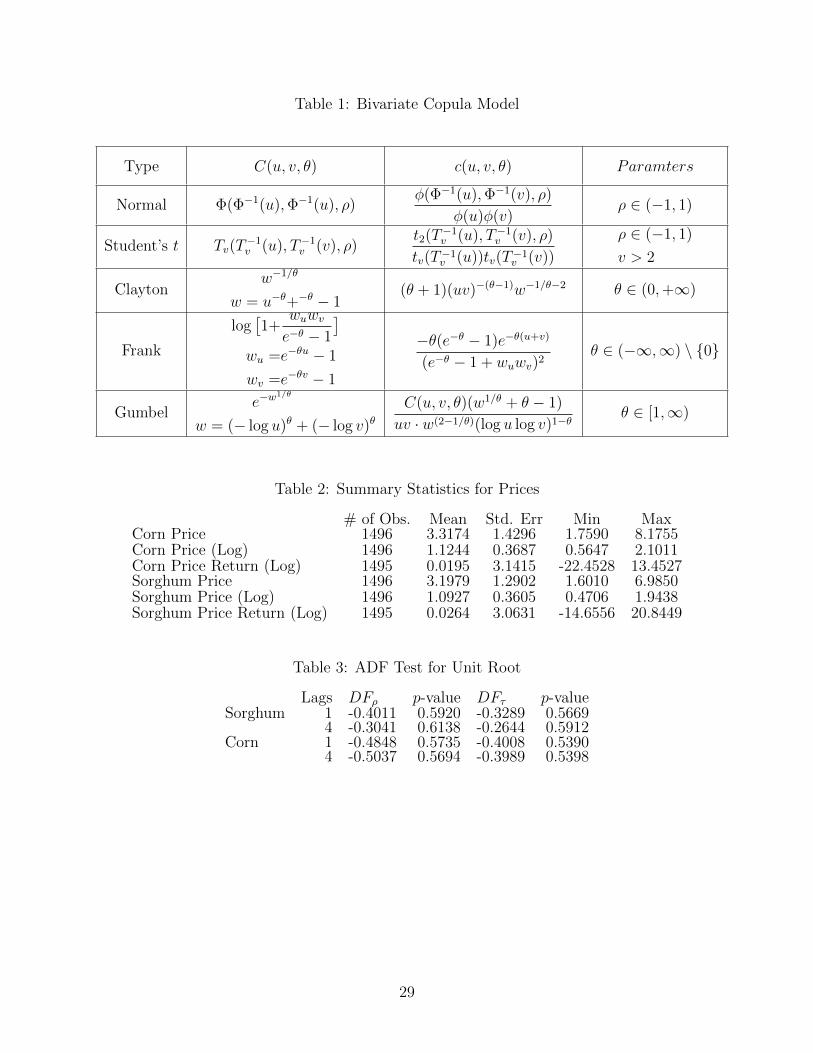
Table 1: Bivariate Copula Model

Type C(u, v, θ) c(u, v, θ) Paramters

Normal Φ(Φ−1(u),Φ−1(u), ρ)φ(Φ−1(u),Φ−1(v), ρ)

φ(u)φ(v)ρ ∈ (−1, 1)

Student’s t Tv(T−1v (u), T−1

v (v), ρ)t2(T−1

v (u), T−1v (v), ρ)

tv(T−1v (u))tv(T−1

v (v))

ρ ∈ (−1, 1)

v > 2

Claytonw−1/θ

w = u−θ+−θ − 1(θ + 1)(uv)−(θ−1)w−1/θ−2 θ ∈ (0,+∞)

Frank

log[1+

wuwve−θ − 1

]wu =e−θu − 1

wv =e−θv − 1

−θ(e−θ − 1)e−θ(u+v)

(e−θ − 1 + wuwv)2θ ∈ (−∞,∞) \ {0}

Gumbele−w

1/θ

w = (− log u)θ + (− log v)θC(u, v, θ)(w1/θ + θ − 1)

uv · w(2−1/θ)(log u log v)1−θ θ ∈ [1,∞)

Table 2: Summary Statistics for Prices

# of Obs. Mean Std. Err Min MaxCorn Price 1496 3.3174 1.4296 1.7590 8.1755Corn Price (Log) 1496 1.1244 0.3687 0.5647 2.1011Corn Price Return (Log) 1495 0.0195 3.1415 -22.4528 13.4527Sorghum Price 1496 3.1979 1.2902 1.6010 6.9850Sorghum Price (Log) 1496 1.0927 0.3605 0.4706 1.9438Sorghum Price Return (Log) 1495 0.0264 3.0631 -14.6556 20.8449

Table 3: ADF Test for Unit Root

Lags DFρ p-value DFτ p-valueSorghum 1 -0.4011 0.5920 -0.3289 0.5669

4 -0.3041 0.6138 -0.2644 0.5912Corn 1 -0.4848 0.5735 -0.4008 0.5390

4 -0.5037 0.5694 -0.3989 0.5398

29

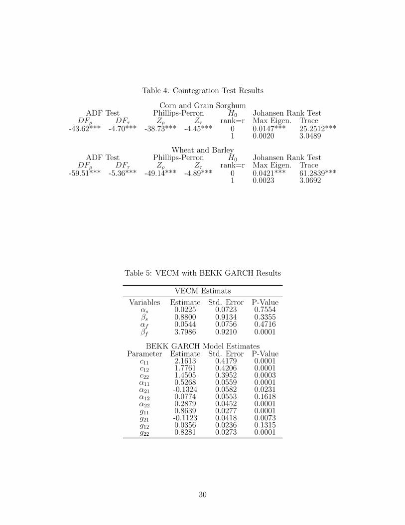
Table 4: Cointegration Test Results

Corn and Grain SorghumADF Test Phillips-Perron H0 Johansen Rank Test

DFρ DFτ Zρ Zτ rank=r Max Eigen. Trace-43.62*** -4.70*** -38.73*** -4.45*** 0 0.0147*** 25.2512***

1 0.0020 3.0489

Wheat and BarleyADF Test Phillips-Perron H0 Johansen Rank Test

DFρ DFτ Zρ Zτ rank=r Max Eigen. Trace-59.51*** -5.36*** -49.14*** -4.89*** 0 0.0421*** 61.2839***

1 0.0023 3.0692

Table 5: VECM with BEKK GARCH Results

VECM Estimats

Variables Estimate Std. Error P-Valueαs 0.0225 0.0723 0.7554βs 0.8800 0.9134 0.3355αf 0.0544 0.0756 0.4716βf 3.7986 0.9210 0.0001

BEKK GARCH Model EstimatesParameter Estimate Std. Error P-Value

c11 2.1613 0.4179 0.0001c12 1.7761 0.4206 0.0001c22 1.4505 0.3952 0.0003α11 0.5268 0.0559 0.0001α21 -0.1324 0.0582 0.0231α12 0.0774 0.0553 0.1618α22 0.2879 0.0452 0.0001g11 0.8639 0.0277 0.0001g21 -0.1123 0.0418 0.0073g12 0.0356 0.0236 0.1315g22 0.8281 0.0273 0.0001

30

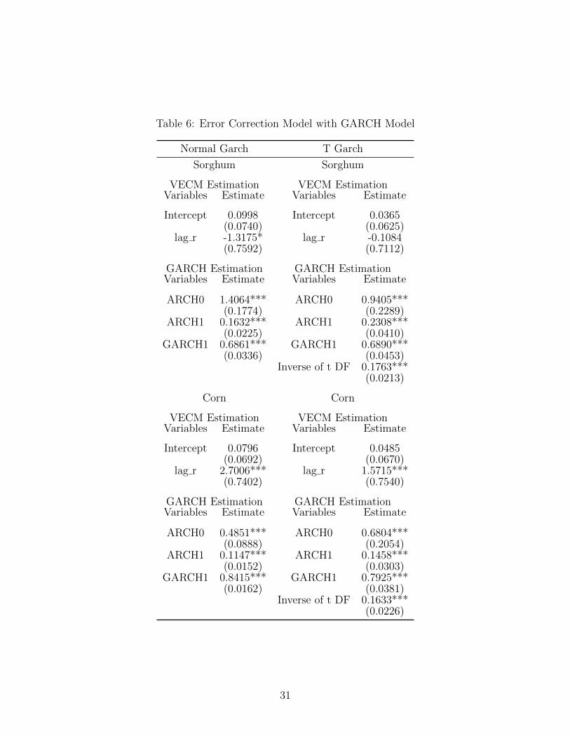
Table 6: Error Correction Model with GARCH Model

Normal Garch T Garch

Sorghum Sorghum

VECM Estimation VECM EstimationVariables Estimate Variables Estimate

Intercept 0.0998 Intercept 0.0365(0.0740) (0.0625)

lag r -1.3175* lag r -0.1084(0.7592) (0.7112)

GARCH Estimation GARCH EstimationVariables Estimate Variables Estimate

ARCH0 1.4064*** ARCH0 0.9405***(0.1774) (0.2289)

ARCH1 0.1632*** ARCH1 0.2308***(0.0225) (0.0410)

GARCH1 0.6861*** GARCH1 0.6890***(0.0336) (0.0453)

Inverse of t DF 0.1763***(0.0213)

Corn Corn

VECM Estimation VECM EstimationVariables Estimate Variables Estimate

Intercept 0.0796 Intercept 0.0485(0.0692) (0.0670)

lag r 2.7006*** lag r 1.5715***(0.7402) (0.7540)

GARCH Estimation GARCH EstimationVariables Estimate Variables Estimate

ARCH0 0.4851*** ARCH0 0.6804***(0.0888) (0.2054)

ARCH1 0.1147*** ARCH1 0.1458***(0.0152) (0.0303)

GARCH1 0.8415*** GARCH1 0.7925***(0.0162) (0.0381)

Inverse of t DF 0.1633***(0.0226)

31

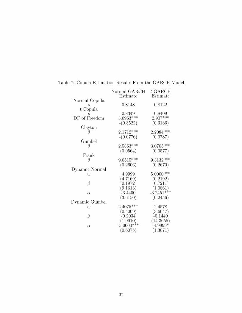
Table 7: Copula Estimation Results From the GARCH Model

Normal GARCH t GARCHEstimate Estimate

Normal Copulaρ 0.8148 0.8122

t Copulaρ 0.8349 0.8409

DF of Freedom 3.0963*** 2.907***-(0.3522) (0.3136)

Claytonθ 2.1712*** 2.2084***

-(0.0776) (0.0787)Gumbel

θ 2.5863*** 3.0705***(0.0564) (0.0577)

Frankθ 9.0515*** 9.3132***

(0.2606) (0.2670)Dynamic Normal

w 4.9999 5.0000***(4.7169) (0.2192)

β 0.1972 0.7211(9.1613) (1.0861)

α -3.4400 -3.2451***(3.6150) (0.2456)

Dynamic Gumbelw 2.4075*** 2.4578

(0.4009) (3.6047)β -0.2034 -0.1449

(1.9910) (14.3655)α -5.0000*** -4.9999*

(0.6075) (1.3071)

32

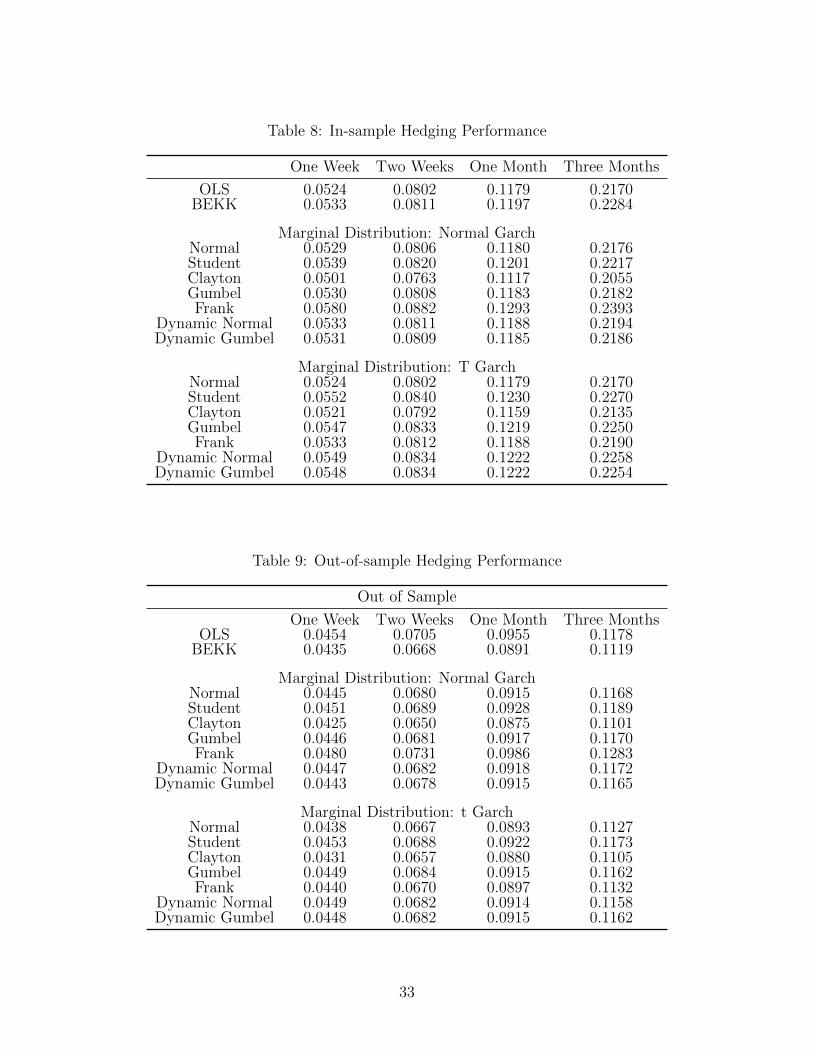
Table 8: In-sample Hedging Performance

One Week Two Weeks One Month Three Months

OLS 0.0524 0.0802 0.1179 0.2170BEKK 0.0533 0.0811 0.1197 0.2284

Marginal Distribution: Normal GarchNormal 0.0529 0.0806 0.1180 0.2176Student 0.0539 0.0820 0.1201 0.2217Clayton 0.0501 0.0763 0.1117 0.2055Gumbel 0.0530 0.0808 0.1183 0.2182Frank 0.0580 0.0882 0.1293 0.2393

Dynamic Normal 0.0533 0.0811 0.1188 0.2194Dynamic Gumbel 0.0531 0.0809 0.1185 0.2186

Marginal Distribution: T GarchNormal 0.0524 0.0802 0.1179 0.2170Student 0.0552 0.0840 0.1230 0.2270Clayton 0.0521 0.0792 0.1159 0.2135Gumbel 0.0547 0.0833 0.1219 0.2250Frank 0.0533 0.0812 0.1188 0.2190

Dynamic Normal 0.0549 0.0834 0.1222 0.2258Dynamic Gumbel 0.0548 0.0834 0.1222 0.2254

Table 9: Out-of-sample Hedging Performance

Out of Sample

One Week Two Weeks One Month Three MonthsOLS 0.0454 0.0705 0.0955 0.1178

BEKK 0.0435 0.0668 0.0891 0.1119

Marginal Distribution: Normal GarchNormal 0.0445 0.0680 0.0915 0.1168Student 0.0451 0.0689 0.0928 0.1189Clayton 0.0425 0.0650 0.0875 0.1101Gumbel 0.0446 0.0681 0.0917 0.1170Frank 0.0480 0.0731 0.0986 0.1283

Dynamic Normal 0.0447 0.0682 0.0918 0.1172Dynamic Gumbel 0.0443 0.0678 0.0915 0.1165

Marginal Distribution: t GarchNormal 0.0438 0.0667 0.0893 0.1127Student 0.0453 0.0688 0.0922 0.1173Clayton 0.0431 0.0657 0.0880 0.1105Gumbel 0.0449 0.0684 0.0915 0.1162Frank 0.0440 0.0670 0.0897 0.1132

Dynamic Normal 0.0449 0.0682 0.0914 0.1158Dynamic Gumbel 0.0448 0.0682 0.0915 0.1162

33

References

Bera, A. K., Garcia, P., and Roh, J. S. (1997). “Estimation of time-varying hedge ratios

for corn and soybeans: BGARCH and random coefficient approaches.” Sankhy: The

Indian Journal of Statistics, Series B, 346-368.

Anderson, R. W., and Danthine, J. P. (1981). “Cross hedging.” Journal of Political Econ-

omy, 89(6), 1182-1196.

Engle, R. F., and Kroner, K. F. (1995). “Multivariate simultaneous generalized ARCH.”

Econometric theory, 11(1), 122-150.

Baillie, R. T., and Myers, R. J. (1991). “Bivariate GARCH estimation of the optimal

commodity futures hedge.” Journal of Applied Econometrics, 6(2), 109-124.

Brown, S. L. (1985). “A reformulation of the portfolio model of hedging.” American Journal

of Agricultural Economics, 67(3), 508-512.

Bollerslev, T. (1986). “Generalized autoregressive conditional heteroskedasticity.” Journal

of econometrics, 31(3), 307-327.

Bollerslev, T. (1990). “Modelling the coherence in short-run nominal exchange rates: a

multivariate generalized ARCH model.” The review of economics and statistics, 498-

505.

Chen, S. S., Lee, C. F., and Shrestha, K. (2004). “An empirical analysis of the relationship

between the hedge ratio and hedging horizon: A simultaneous estimation of the short-

and long-run hedge ratios.” Journal of Futures Markets, 24(4), 359-386.

Dickey, D.A. and Fuller, W.A., (1979). “Distribution of the estimators for autoregressive

time series with a unit root.” Journal of the American statistical association, 74(366a),

pp.427-431.

34

Engle, R. F. (1982). “Autoregressive conditional heteroscedasticity with estimates of the

variance of United Kingdom inflation.” Econometrica: Journal of the Econometric

Society, 987-1007.

Engle, R. F., and Kroner, K. F. (1995). “Multivariate simultaneous generalized ARCH.”

Econometric theory, 11(1), 122-150.

Engle, R. F., and Sheppard, K. (2001). “Theoretical and empirical properties of dynamic

conditional correlation multivariate GARCH (No. w8554).” National Bureau of Eco-

nomic Research.

Hayenga, M. L., and DiPietre, D. D. (1982). “Cross-hedging wholesale pork products using

live hog futures.” American Journal of Agricultural Economics, 64(4), 747-751.

Headey, D., and Fan, S. (2010). Reflections on the global food crisis: how did it happen?

how has it hurt? and how can we prevent the next one? (Vol. 165). Intl Food Policy

Res Inst.

Herbst, A. F., Kare, D. D., and Marshall, J. F. (1989). “A time varying, convergence

adjusted hedge ratio model.” Advances in Futures and Options Research, 6, 137-155.

Hsu, C. C., Tseng, C. P., and Wang, Y. H. (2008). “Dynamic hedging with futures: A

copulabased GARCH model.” Journal of Futures Markets, 28(11), 1095-1116.

Kahl, K. H. (1983). “Determination of the recommended hedging ratio.” American Journal

of Agricultural Economics, 65(3), 603-605.

McCuistion, Kim (2014). “Nutritional Guide to Feeding Sorghum” Retrieved from: http://www.sorghu

mcheckoff.com/assets/media/exportsorghumpresentations/Kim-McCuistion Livestock ExportSorghum2014.PDF

Myers, R. J. (1991). “Estimating timevarying optimal hedge ratios on futures markets.”

Journal of Futures Markets, 11(1), 39-53.

Nelsen, R. B. (2007). “An introduction to copulas.” Springer Science and Business Media.

35

Patton, A. J. (2006). “Modelling asymmetric exchange rate dependence.” International

economic review. 47(2), 527-556.

Phillips, P.C. and Perron, P., (1988). “Testing for a unit root in time series regression.”

Biometrika, 75(2), pp.335-346.

Power, G. J., Vedenov, D. V., Anderson, D. P., and Klose, S. (2013). “Market volatility

and the dynamic hedging of multi-commodity price risk.” Applied Economics, 45(27),

3891-3903.

Rodriguez, J. C. (2007). “Measuring financial contagion: A copula approach.” Journal of

empirical finance, 14(3), 401-423.

Rusche Warren (2015), “Feeding Sorghum Crops as Alternatives to Corn.” Retrieved from:

http://igrow. org/livestock/beef/feeding-sorghum-crops-as-alternatives-to-corn/

Sklar, M. (1959). “Fonctions de repartition an dimensions et leurs marges.” Publ. Inst.

Statist. Univ. Paris, 8, 229-231.

Van Den Goorbergh, R. W., Genest, C., and Werker, B. J. (2005). “Bivariate option

pricing using dynamic copula models.” Insurance: Mathematics and Economics, 37(1),

101-114.

Witt, H. J., Schroeder, T. C., and Hayenga, M. L. (1987). “Comparison of analytical ap-

proaches for estimating hedge ratios for agricultural commodities.” Journal of Futures

Markets, 7(2), 135-146.

Wu, C. C., Chung, H., and Chang, Y. H. (2012). “The economic value of co-movement

between oil price and exchange rate using copula-based GARCH models.” Energy Eco-

nomics, 34(1), 270-282.

Zhao, J., and Goodwin, B. K. (2012, August). “Dynamic Cross-Hedge Ratios: An Ap-

plication of Copula Models.” In 2012 Annual Meeting, August 12-14, 2012, Seattle,

Washington, (No. 124610). Agricultural and Applied Economics Association.

36

Johansen, S. and Juselius, K., (1990). “Maximum likelihood estimation and inference

on cointegrationwith applications to the demand for money.” Oxford Bulletin of Eco-

nomics and statistics, 52(2), pp.169-210.

37