


Languages
Pages
Legal


Credit, the Stock Market and Oil:Forecasting U.S. GDP
JOHN MUELLBAUER(Nuffield College, University of Oxford, England)
and
LUCA NUNZIATA(Nuffield College, University of Oxford, England)
June 12, 2001
* This research was supported by the Economic and Social Research Council, under grant numberR000237500. We are grateful to Cara Lown for help in extracting historical data from the Federal ReserveSurvey of Senior Loan Officers and to Janine Aron, Spencer Dale, David Hendry, Nick Oulton, AdrianPagan, Neil Shephard, Simon Ward and seminar participants in Oxford and the Bank of England for helpfulcomments.
1
Abstract:
We derive a comprehensive one-year ahead forecasting model of U.S. per capita GDP for 1955-2000, examining collectively variables usually considered singly, e.g. interest rates, creditconditions, the stock market, oil prices and the yield gap, of which all, except the last, are found tomatter. The credit conditions index is measured in the Federal Reserve’s Survey of Senior LoanOfficers and its importance is consistent with a ‘financial accelerator’ view. The balance ofpayments, exchange rate and fiscal policy also play a role. We address the Lucas critique,investigating consequences of monetary policy regime shifts in 1980, and fiscal policy regimeshifts at the end of the 1980’s. The model forecasts the most severe growth reversal in 2001 since1974.
JEL codes: E63. E32, E37
Keywords: macroeconomic forecasts, monetary policy transmission, the credit channel, thefinancial accelerator, Lucas critique, the U.S. recession, oil prices.

2
1. Introduction
There has been a remarkable shift in perceptions of the U.S. economic outlook between the summer
of 2000 and the beginning of 2001. The business cycle has returned with a vengeance when some
believed that the ‘new economy’ based on the internet and other new technologies had abolished it
permanently. Though there is evidence of a regime shift in the period 1989-92, we find little
evidence of shifts since then in relationships governing the cyclical pattern in U.S. GDP. However,
the nature of these relationships should be more widely appreciated, particularly as they now point
to one of the sharpest downturns in the U.S. business cycle in the post-war period.
There is extensive published research on forecasting U.S. GDP growth. Much of this literature has
been concerned with an interest in a specific hypothesis such as the influence of monetary policy,
credit conditions or the financial accelerator, stock market prices, oil prices, yield spreads and the
yield curve on growth. Typically, these questions have been examined in the context of a narrow,
often bivariate VAR. To be fair, much of this work has been less concerned with practical
forecasting than with finding evidence for or against some hypothesis.
Another strand of literature is concerned with shifts in the underlying process governing the
business cycle, following the work of Hamilton (1989) on Markov switching models. In two-state
versions of these models, it is argued that there is a parameter shift in the dynamics between
‘recession’ and ‘recovery’ phases of the business cycle. The bulk of this work, while
econometrically sophisticated, has been in a univariate context, though, more recently, Hamilton
and Lin (1996) have examined the joint behaviour of stock returns and growth, and Krolzig and
Toro (2000) have examined models incorporating information on oil prices and unemployment,
where the stochastic process for GDP shifts.
In this paper, we derive a more comprehensive forecasting model for 1955-2000 examining the
above influences, but in a wider macroeconomic context where the balance of payments, the
exchange rate and fiscal policy also play a role. Moreover, we take seriously the Lucas critique
and explore possible consequences of shifts in the monetary policy regime around 1980, see
Clarida, Gali and Gertler (1998) and of the fiscal policy regime around 1989, see Muellbauer
(1996). We show that, in a range of models, an index of credit conditions as measured in the

3
Federal Reserve’s Survey of Senior Loan Officers, a real stock market price index, an index of real
oil prices and/or the rise of inflation over recent levels, have important predictive power, in
addition to the short-term interest rate, reflecting monetary policy, and the three macro variables
mentioned above. We find that an important shift in behaviour occurred around 1989, consistent
with the Lucas critique.
The model is for annual GDP growth but incorporates higher frequency information available in
early January as well as information in the form of annual averages. Though the form of the model
is a single forecasting equation, a conventional quarterly econometric model or VAR would need at
least a dozen behavioural equations to produce comparable four-quarter ahead forecasts. Stability
tests suggest that, despite the rich specification, parameter stability in the last two decades has been
remarkably good, once the influence of the regime shift in fiscal policy is incorporated.
Section 2 briefly reviews some of the previous literature and provides some theoretical background
for our more comprehensive model. The Federal Reserve’s Senior Loan Officer Survey was
carried out quarterly between 1967 and 1983 and from 1990 to the present. The Appendix derives
quarterly econometric models for interpolating the missing observations. Section 3 presents
evidence for a range of one-year ahead forecasting model using data in the form of annual averages
for the period 1955-1999 plus information from the last quarter or month of each year. In some of
these models, only linear trends appear, but we also investigate alternatives which incorporate
stochastic trends estimated via Koopman et al’s (2000) STAMP package to capture the long-run
evolution of the economy and check further robustness issues. Section 4 discusses some of the
economic context of 2001 further and concludes.
2. The Economic Background
Important results on output forecasting arise in the context of empirical work on the monetary
transmission mechanism. Economic theory suggests higher interest rates curtail consumer and
investment spending impacting both directly and via their indirect effects on asset values and
income expectations. Many studies use VAR’s to examine effects of short-term interest rates or
other monetary policy indicators on subsequent output growth, see Sims (1980, 1987, 1996), Todd
(1990), and Bernanke (1990). More recently, attention has been given to the ‘credit channel’,

4
Bernanke and Blinder (1992), Bernanke and Gertler (1995) or the ‘financial accelerator’, Bernanke,
Gertler and Gilchrist (1996, 1999). In this framework, the credit terms available to firms depend on
the source of finance (e.g inside vs. outside finance) and the terms of such finance can vary with
economic conditions. For example, a fall in a firm’s net worth reduces the effective collateral a
bank may be able to access in the event of a loan default. Changes in asset prices are thus likely to
influence credit terms. More generally, increased uncertainty, a downturn in the economic outlook
or a fall in the net worth of banks themselves can all influence the cost of outside finance available
to firms by altering the willingness or ability of banks to provide such finance. Some empirical
research has proxied credit conditions using spreads between corporate and government bonds as
one proxy for such credit terms, see Gertler and Lown (1999), though others have interpreted such
spreads instead as a proxy for uncertainty. In what follows, we examine the impact both of short-
term interest rates and credit conditions, as measured by the Federal Reserve survey.
Asset prices obviously play an important role in the transmission mechanism, whether one takes a
‘conventional’ asset markets view, see Taylor (1999), or the credit channel view. Research has
examined the effects of asset prices and asset price volatility on GDP growth, see Hamilton and Lin
(1996) and Estrella and Mishkin (1998). Another financial variable, which has received much
attention as a predictor of cyclical activity (as well as of inflation), is the yield curve or the yield
gap between short-term and long-term bonds, see Campbell (1995), Estrella and Mishkin (1998),
Bernard and Gerlach (1998), and Peel and Taylor (1997).
Finally, the effects of oil prices on the economy have been much studied, see Hamilton (1983),
Mork (1989), Hooker (1996), Ferderer (1996), Raymond and Rich (1997), and Clements and
Krolzig (2001). Considerable attention has been given to possible asymmetries in these effects,
where increases in oil prices damage growth more than decreases in prices benefit growth.
We will embody the above credit, monetary transmission, asset and oil price variables in a more
general macroeconomic framework. Following Muellbauer (1996), output growth is captured in a
dual adjustment process: firstly, of output to equilibrium output given by an income - expenditure
model and secondly, of output to trend output. Trend output is determined, in principle, by the
state of technology and physical and human capital stocks. The adjustment process involves
spontaneously occurring recovery forces operating in recessions. These might include real wages
and real raw material prices falling far enough relative to productivity trends to make production,

5
employment and investment more profitable again, as well as rising replacement demand and low
interest rates resulting from the low investment rates associated with recession. The reverse
mechanisms operate in booms, together with the high marginal costs associated with overtime hour
premia and, in the limit, sheer capacity or labour supply constraints. Large macroeconometric
models articulate many elements of these processes. In what follows they will be summarized by a
single adjustment equation.
In this equation, three variables capture the self-correcting tendency of growth to fall after final
expenditure has overshot capacity and to recover when output is below capacity. The first of these
is the deviation of output from trend (though we have also examined specifications in which this is
replaced by the unemployment rate). The second is the trade balance to GDP ratio, since excess
demand spills over into higher imports. And the third is the deviation of inflation from average
inflation in recent years. Empirical research on U.S. inflation, see Stock and Watson (1999),
emphasizes the role of the output gap in explaining inflation. It makes sense therefore to
investigate this kind of inflation effect as another symptom of over- or undershooting of GDP.
In what follows, we consider the rich set of variables discussed above to capture influences on
autonomous demand, including real and nominal interest rates, the government bond yield gap, an
index of credit conditions, real stock market prices and the real exchange rate.
A distinction can be made between the structural adjustment process with policy in neutral, and the
solved out adjustment process incorporating policy feedback rules. These reflect policymakers’
dislike of inflation shocks and of too high unemployment, as well as their possible concerns for
balancing government budget and trade accounts. Because the actually observed solved out
adjustment process is a mixture of the process that would hold for the private sector with inactive
policy and the policy feedback rules of the policymakers, it is likely to shift when policymakers’
preferences shift. In other words, the forecasting equation will implicitly incorporate monetary and
fiscal policy feedback rules and, in principle, is therefore subject to the Lucas critique.
The dual adjustment process mentioned above can be articulated as follows. When goods markets
are in equilibrium GDP (Y) equals total expenditure, consumption (C) + investment (I) +
government expenditure on goods and services (G) + exports (X) - imports (M). Suppose private
expenditure depends linearly on GDP minus taxes plus an autonomous element A which reflects,

6
for example, interest rates, wealth, the real exchange rate, uncertainty and growth expectations.
Then, in goods market equilibrium, equilibrium GDP, denoted by Y* is given by:
* ( * )Y a Y T A G X M= − + + + − (1)
so that
1* [ ]
1Y A G aT X M
a= + − + −
−(2)
1[ ]
1A G T X M
a≈ + − + −
−
if a is of the order of 0.8 or more.
There is also some process of adaptation of GDP to trend income (TY), depending on the level of
*technology, human and physical capital.
Suppose there is an adjustment mechanism linking actual Y both with Y* and with trend Y:
*1 1 2 1 1 3 1 1( * ) ( ) ( )t t t t t t tY b Y Y b Y Y b TY Y− − − − −∆ = − + − + − (3)
Note that b2 > 0 captures the idea that the adjustment process could be drawn out enough so that
last period’s deviation of output from the equilibrium level continues to exert some influence this
period. Deflating by Yt-1 gives the log approximation:
** * * *0 1 2 3 1 1
11
*ln (ln ln )t
t t ttt
Y YY b b b b TY Y
Y Y − −−−
∆ ≈ + + + −
(4)
where lnTYt-1 - lnYt-1 corresponds to the usual concept of an output gap.
Let -(G-T)/Y be denoted GSUR, ie., the government surplus to GDP ratio and -(X-M)/Y be
denoted TDEF, ie., the trade deficit to GDP ratio. Then (4) becomes
7
* ** 11 20 1 1
1 1
ln [ ] [( ) ]1 1
t tt t t t t
t t
A Ab bY b GSUR TDEF GSUR TDEF
a Y a Y−
− −− −
∆ ≈ + − − + − −− −
*3 1 1(ln ln )t tb TY Y− −+ − (5)
Equation (5) is the economy’s approximate structural adjustment equation and becomes a
forecasting equation when1
[ ]tt t
t
AGSUR TDEF
Y −
− − is replaced by variables dated t-1 which forecast
this term. This forecast will implicitly incorporate monetary and fiscal policy feedback rules and,
in principle, is therefore subject to the Lucas critique. In what follows, we consider a rich set of
variables to capture influences on autonomous demand including real and nominal interest rates,
the government bond yield gap, an index of credit conditions, real stock market prices and the real
exchange rate.
As noted above, the output gap lnTYt-1 - lnYt-1 may not be well measured as the deviation of log
GDP from a linear trend. The deviation of inflation from levels in recent years and the trade deficit
to GDP ratio, TDEF, are likely to provide additional information on the output gap. Lags in TDEF
may therefore reflect persistence in TDEFt-1 which helps forecast TDEFt, the direct role of TDEFt-1
envisaged in eq(5) and an indirect role via its contribution to measuring the output gap.
The 1980’s saw increasing international concern among macroeconomists and latterly policy
makers about the long-run sustainability of fiscal policy, see Federal Reserve Bank of Kansas City
(1995) and Bryant et al (1993). Correspondingly, in the US, there was a shift in the attitude of
policymakers to the federal government’s budget deficit. This was signalled by the passing in late
1985 of the first of the Gramm-Rudman Amendments. However, most observers, e.g. White and
Wildavsky (1991), see especially the Postscript, agree that the Budget Enforcement Act of 1990
was the most important milestone. This appears to be the key shift in the fiscal policy feedback
rule since the 1950’s and also coincides with the end of the Cold War, and the decline in defense
spending which followed.
As far as shifts in the monetary policy feedback rule are concerned, Clarida, Gertler and Gali
(1998) argue that 1980 marks the key shift. Under Federal Reserve chairmen Volcker and
Greenspan, the Federal Reserve became more committed to fighting inflation. Estimates of
8
extended Taylor rules suggest that, from 1980, a rise in inflation was followed by an even greater
rise in nominal interest rates so that real interest rates rose, while this was not so before 1980.
Below, we test for both of these regime shifts.
3. An Annual Model of Per Capita U.S. GDP Growth
At the beginning of each year, the media and stockbrokers’ reports predict the economic outlook
for the coming year. It is reasonable to want to forecast the annual average of GDP relative to last
year’s annual average. One can consider several different information sets for forecasting. One
consists just of annual average data, which gives the broad picture of business cycle dynamics for
the last 45 years. If last year’s annual average of data drawn from the national accounts is in the
information set, this strictly speaking, means that forecasts cannot be made until end-January, when
the 4th quarter data from the national accounts are published – unless the 4th quarter data are
themselves forecast. Confining oneself to data in annual average form, however, is unnecessarily
restrictive. A wider information set therefore supplements these data with information available at
the beginning of each year about the last month or quarter of each year. We therefore consider the
deviation of available monthly or quarterly data from the annual average.
Our dependent variable is DLGDP(t+1), the annual growth rate of U.S. real GDP minus
DLWAPOP(t), the growth rate of the working age population one year earlier. The reason for this
form of the dependent variable is that this year’s growth rate of the working age population is the
best simple forecast of next year’s. All regressors in the model are dated t or earlier, reflecting an
information set up to January of year t+1. An important feature of our model is the tendency of
output growth to correct recent supply-demand imbalances. As noted earlier, we include three
measures of such imbalances. The first is an output gap. One measure of the output gap is the
deviation from trend of real log GDP scaled by working age population.1 Our model therefore
includes LGDPW (log per capita GDP) and the trend. The second measure of supply-demand
imbalances is the trade deficit-to-GDP ratio, TDEF. The final measure is the deviation of inflation
in year t from recent average inflation rates, INFLD, where we take average inflation in the
previous four years, t-1 to t-5, as the relevant indicator. Research on U.S. inflation, e.g. by Stock

9
and Watson (1999), has emphasized the importance of supply-demand imbalances on the inflation
deviation, so it seems useful to take the deviation of inflation as an additional indicator of such
imbalances.
As well as the tendency towards correcting such imbalances, a kind of trend reversion or
‘equilibrium correction’, it seems likely that GDP also has short-term momentum or persistence.
Thus end-of-year news about the cyclical position of the economy is likely to make a useful
contribution to forecasting the annual average of GDP.2 We find the deviation of weekly hours of
work in the last quarter from the annual average, WHDLQ, to be very informative in this respect
and this measure is available on the first Friday of January, and is not usually subject to significant
revision.
Our other regressors include a range of financial and credit variables likely to influence
autonomous demand (i.e. separately from the effects of current income on demand). These are the
change in the nominal 3-month Treasury bill rate, DIR, the level of the real short-term interest rate,
RIR defined as the T-bill rate minus current CPI inflation, the index of tighter loan standards from
the Federal Reserve’s quarterly Survey of Senior Loan Officers of around eighty major banks, TLS,
the log S&P stock price index deflated by the CPI, LSP, a measure of stock market volatility,
STOVOL, and the yield gap defined as the yield on one-year Treasury bonds minus the yield on
ten-year treasury bonds. The other variables are the log real oil price index, LOILP or its deviation
from its lagged 5-year moving average, DEVOIL, the log real exchange rate, LREER, the primary
federal government budget surplus to GDP ratio, GSUR, and the federal government debt to GDP
ratio, GDEBT. The reason for including the nominal interest rate in difference form lies in the fact
that in a potential high inflation period, when nominal rates are high, one would not necessarily
expect growth to be low for that reason.3
End-of-year news about some of these variables might be expected to contribute to forecasting
annual GDP in the following year. So we check whether the difference between the December
1 For the U.S., (minus) the unemployment rate is a good alternative proxy for this. It also has the advantage of beingavailable by the second week of January, while GDP data only come in later and are subject to considerable revision.We therefore present alternative versions of our models, which use the unemployment rate as the output gap proxy.2 As is well known, GDP is very persistent in quarterly data. The persistence of LGDPC as measured in a simple ARIprocess will be considerably higher at a one-quarter gap than at a four-quarter gap. If the regression coefficient of Yt
as Yt-1 is b on quarterly data, it should be about b4 in the regression of Yt on Tt-4 or in the analogous regression onannual data.3 Hendry (1995) uses the term ‘congruent’ to describe this type of constraint on a feasible model.

10
value and the annual average of the T-bill rate, the index of tighter loan standards, the stock price
index and the oil price have any forecasting potential.
Two regime shifts were discussed in the previous section. To handle the possible shift in the
monetary policy regime in 1980, we define a step-dummy D80 to be zero up to 1979 and one from
1980. We then interact it with current and lagged values of our interest rate variables. To handle
the fiscal policy regime shift in 1989, we use the dummy variable used for a similar purpose4 in
Muellbauer (1996). To phase the shift in gradually, we define D89 to be zero up to 1988, 0.25 in
1989, 0.5 in 1990, 0.75 in 1991 and 1 from 1992 onwards. We then interact this with current and
lagged values of GSUR and with GDEBT5. We might expect GSUR to have the conventional
Keynesian effect on output growth up to 1988: the larger the surplus, the less short-term growth,
implying a negative coefficient on GSUR. From 1989, we expect this effect to weaken or reverse
as surpluses are increasingly seen as a signal for lower taxes or greater spending in the future,
making consumers and businesses more optimistic. Similarly, once the private sector realized that
the federal government was seriously concerned about the government debt to income ratio, one
would expect high levels of this debt to have a negative influence on future growth. The Data
Appendix summarizes the terminology and data sources.
Even with only two lags, i.e. information dated t and t-1, the general model is very rich, at least by
typical North American econometric practice. However, recent literature on ‘general to specific’
model selection procedures, see Hoover and Perez (1999), Hendry (2000) and Hendry and Krolzig
(1999), suggests that sensible model selection procedures, using a variety of criteria, including fit,
lack of residual autocorrelation and parameter stability, can select parsimonious reductions which
are surprisingly free of ‘pre-test bias’ problems6. Moreover, we have plausible priors for all the
signs of the explanatory variables, given the theoretical framework and standard economics, which
predicts that higher interest rates, tighter loan conditions, a more overvalued real exchange rate, a
fall in the stock market and higher oil prices all reduce next period’s growth.
Our reduction procedure operates in two steps. First, we check that in the general model there are
no significant effects contradicting these sign priors. This turns out to be true. Then we eliminate
4 But to forecast personal non-property income per head.5 Since GSUR is closely related to changes in GDEBT, we only include the t-dated value of GDEBT in the generalequation.

11
insignificant ‘wrong-signed’ effects. To protect against the possibility of omitting t-2 dated
effects, we look for significant t-1 dated effects. Whenever we find one, we add the t-2 effect for
that variable. With this temporarily expanded model, we now follow again a ‘general to specific’
model selection strategy. Log GDPW appears as a two-year moving average LGDPWMA. The
trade deficit to GDP ratio appears as a lagged two year moving average. This is the only variable
where a t-2 dated effect appears. One interpretation of the lack of significance of a t-dated effect is
that the two other indicators of supply-demand imbalances, the deviation from trend of output and
the deviation of inflation from levels in recent years, mop up the t-dated supply-demand imbalance.
It is also likely that switching costs imply considerable hysteresis in trade patterns.
The yield gap is always insignificant. The real interest rate effect appears as a first difference and
the difference of the nominal interest rate is insignificant. The index of tighter loan standards, the
real stock market index and the real oil price are significant as current levels though its deviation
from its five-year moving average, DEVOIL, fits best as a two-year moving average, DEVOILMA.
Stock market volatility, using monthly data, appears to enter as a two-year moving average. The
December deviation of the real stock market index from the annual average, LSPD is also quite
important. It is most significant in the form of an annual difference, DLSPD.
Regarding potential policy shifts, we find slight evidence, but not statistically significant, that
before 1980, changes in nominal rates had somewhat stronger negative effects, while from 1980,
changes in real rates had somewhat stronger negative effects.7 The fiscal policy shift, however, in
1989 is strongly significant and can be simply represented by interacting our D89 dummy with
government debt/GDP, represented as GDEBT*D89. The government surplus to GDP ratio,
GSUR does have a negative coefficient before 1989 and a positive one from the early 1990’s, but
neither effect is significant. The effect of GDEBT*D89 implies a significant slowing of economic
growth from 1989, though as government debt is reduced in later years, this negative effect tends to
wear off. We cannot rule out the possibility that other factors might be contributing to this effect,
for example, over-investment in the late 1980’s in commercial real estate, which led to a long
6 In which the investigator mis-states the size of the test, so increasing the risk of choosing to include variables not inthe data generation process, which happen to have a sample correlation with the dependent variable.7 However, note that in the Appendix, we find evidence of a shift in the determinants of the index of tighter loanstandards, TLS. Indeed, there is evidence that from 1980, a higher level of real interest rates raises TLS.

12
slump in this market and contributed to low rates of investment in the early 1990’s, see further
discussion later.8
Some results are shown in Table 1 and the last row shows the implied forecast growth rate of GDP
(NOT in per capita form). Column 1 of Table 1 shows one of our best-fitting parsimonious
specifications estimating for 1955-88. Column 2 shows estimates for 1955-95 and column 3 for
1955-99. Parameter stability looks satisfactory. The growth forecast for 2001 is for a 0.6%
contraction. Compared with 4.8% growth in 2000, this is a striking change.
We know that the American economy has become more open in the last 35 years: the ratio of non-
oil imports to GDP has risen steadily from under 3% in 1965 to over 11% in 2000. This suggests
that the responsiveness of output growth to the real exchange rate has increased over time.
Recursive estimates of the parameters suggest that the real exchange rate coefficient has indeed
become more negative. In column 4, we therefore display a specification in which the deviation of
LREER from its 1965 value is interacted with a split trend which is zero up to 1965, 1 in 1966, 2 in
1967 etc., giving the variable denoted LREER*. LREER then has a coefficient of effectively zero
(t ≈0.3) and can be omitted. This specification fits a little better than that of column 3.
Lagrange multiplier tests for residual autocorrelation at lags up to two years are shown in the
penultimate row of Table 1 and are satisfactory. Tests for heteroscedasticity and normality of the
residuals are always satisfactory.
The assumption that the deviation of output from a linear trend is a good representation of the
output gap seems a strong one and is worth checking for non-linearities. We therefore re-
estimated these equations using the STAMP software of Koopman et al (2000), which uses Kalman
filtering to estimate a stochastic trend. This, however, confirms the linear trend.
Perhaps the most controversial aspect of our model arises through the GDEBT*D89 term, which as
noted above, implies a strong growth slowdown from 1989 into the 1990’s. If we omit this term
and re-estimate the model in STAMP, we obtain the results shown in Table 1, column 6. The
8 Incidentally, if we include a ‘capital deepening measure’ defined as the log of the real capital stock relative toworking age population, this typically has a negative but insignificant coefficient. One interpretation is thatoverinvestment has demand consequences that, on average, overcome the contribution of the capital stock to trendoutput, given that a linear time trend is included in the equation.

13
stochastic trend now estimated by STAMP is specified as an I(1) stochastic intercept and shows a
sharp slow-down in growth after 1989, followed by the resumption of trend growth at broadly
similar rates several years later, see Figure 3. The stochastic trend can be thought of as a slightly
smoothed estimate of the effect of omitted I(1) variables which therefore ‘robustifies’ the
forecasting procedure: the one year ahead forecast assumes that the I(1) component remains the
same at t+1 as at t. With the exception of the coefficient on LTDEFMA(t-1), the parameter
estimates are similar to those shown in columns 1 to 4. The forecast growth rate in 2001 is –1.0%
%, marginally worse than the other columns, despite the lower coefficient on LTDEFMA(-1).
However, if we estimate up to 1988 using STAMP, the coefficient on TDEFMA(t-1) rises to the
levels found in columns 1 to 4, see column 5. In other words, parameter stability is better for the
specifications incorporating GDEBT*D89 than for those omitting it.
We show recursive estimates, computed in Doornik and Hendry’s (1998) PCGIVE, of the beta
coefficients and the recursive Chow test for a structural break for the column 3 specification in
Figure 1. The Chow test tests the hypothesis of a structural break between the point in the sample
at t and the end of the sample. Parameter stability looks satisfactory once the shift in the fiscal
policy reaction function in 1989 is allowed for. Omission of the inflation effect results in a worse
fit but a much more significant oil price effect before and after 1979.
Let us now consider the orders of integration of the data. Augmented Dickey-Fuller tests suggest
that the I(0) variables in the data set are per capita output growth, the interest rate changes and the
last month deviation in the stock price index and in weekly average hours of work. The remainder,
the output gap, the debt to GDP ratio, the trade deficit to GDP ratio, the real exchange rate, the real
stock market price index and the index of tightening loan standards all appear to be I(1). The
model suggests at least one co-integrating relationship between these variables. Given the
structural break in 1989, applying formal procedures such as the Johansen procedure to investigate
cointegration for the full sample is difficult. On the other hand, applying it to the period 1955-88
with such a rich set of variables is likely to result in tests that lack power.
An indication of the contribution of each of the regressors to the change in U.S. log GDP is found
in Figures 2a, 2b and 2c, which weight each variable by its estimated coefficient using Table 1,
column 3. This provides interesting historical decompositions of U.S. business cycle fluctuations.
The contribution of the rising stock market and the falling government debt to GDP ratio in the
14
second half of the 1990’s is notable. Note that the recursive estimates shown in Chart 1, for the
two stock market effects, LSP and DLSPD, suggest that the estimated coefficients have been stable
for 20 years9 and are not merely picking up some chance correlation between the stock market and
growth in the late 1990’s. However, this conclusion may depend on the interpretation of the 1990-
91 recession.
We have also investigated the use of a broader measure of wealth than the stock market index using
the Federal Reserve’s household balance sheets for the end of each year. The models always fit
less well but give broadly similar forecasts.
In Table 2, we show comparable specifications, which use the unemployment rate UR instead of
LGDPWMA. Shimer(1998) argues that the average unemployment rate is distorted as a measure
of supply-demand imbalances by variations in the age composition of the labour force. As is well
known, unemployment rates for recent entrants to the labour market tend to be higher. We
therefore included the proportion of the labour force aged 16-24, LFYT, which peaks in the early
1980’s, to correct for this. Indeed, its lagged value has a significant negative coefficient and the
goodness of fit of these equations is comparable to those in Table 1, though both the oil price and
stock market volatility have weaker effects. Kalman filter estimates using the STAMP package and
an I(1) specification of a stochastic level effect give the results shown in columns 5 and 6. As in
the comparable column in Table 1, GDEBT*D89 is omitted in column 6 with comparable results.
The forecasts for 2001, shown in the last row of Table 2, are for 0.1% or zero growth in columns 3
and 4 and for -0.2% growth in column 6.
The 1990-91 Recession and Its Aftermath
One of the puzzles in U.S. post-war business cycle history is the 1990-91 recession and the
relatively slow recovery, which followed it. Blanchard (1993) suggests a proximate cause in the
decline of consumption and non-residential investment but offers little explanation for why these
occurred, aside from the observations that consumer confidence remained low for two years after
the invasion of Kuwait in August 1990. Hall (1993) considers a wide range of possibilities
including a rise in marginal tax rates, a negative productivity shock, a credit crunch afforced by
9 Note that since LSP and DLSPD have similar coefficients, these two effects can be reparameterized as the twoyear moving average of the log real S&P index and its annual December to December change.

15
tighter bank regulation and a spontaneous decline in consumption, reflecting lower income
expectations. Walsh (1993) also put a large weight on a shift in the IS curve using evidence from a
quarterly VAR of output, inflation, the T-bill rate and M2 but without, in turn, explaining this.
Bernanke and Lown (1991) investigate the credit crunch hypothesis in some depth, providing
evidence that it played a significant role in the 1989-90 downturn. Hansen and Prescott (1993)
raise the possibility of a downturn in the growth of productivity.
Perhaps the most suggestive interpretations emerge in a series of papers by Runkle (1990, 1991,
1992). He provides evidence from the Bayesian vector autoregression (BVAR) model at the
Minnesota Federal Reserve developed by Doan, Litterman and Sims (1984), see also Litterman
(1984). Runkle also draws heavily on ancillary information. In his 1991 paper he notes that the
period since 1989 had seen the second weakest consumption growth since 1948. Among factors he
cites are the government budget constraint - the fiscal plight of state and local as well as the Federal
government, and the possibility that with the rise of labour participation and hours in the 1980’s,
households were now anticipating a slower rise in permanent income. He suggests that the
weakness of the residential property market also helps explain weak consumption growth, though
he finds no evidence for a forecasting role for house prices in the Minnesota Fed’s forecasting
model. Like Bernanke and Lown (1991), he notes the decline in the commercial real estate market
which was holding back non-residential investment.
Our models shown in Table 1, columns 2 to 4, place a large weight on the regime switch in fiscal
policy between 1989 and 1992. Figure 2a makes clear that the trough in growth occurred in 1991.
While tighter loan standards (TLS) reflecting the credit crunch in 1990, see Figure 2b, and the
decline in the stock market at the end of 1990 (DLSPD), see Figure 2c, help explain the down-turn,
there are also important offsetting factors, particularly the improvement in the trade deficit relative
to GDP, TDEFMA(-1), see Figure 2a.10 In our model, the fall in GDEBT*D89, thus contributes an
important missing link. Furthermore, the continued decline in this term to 1992 helps explain why
the pick-up in GDP growth from 1991 to 1993 was not more dramatic given the positive
contribution of the output gap, the improved trade deficit relative to GDP, lower inflation, easier
loan standards, lower oil prices, a rising stock market and even the rise in weekly hours at the end
of 1991. The GDEBT*D89 term provides one explanation for the decline in consumption noted by
10 To which both the fall in the real exchange rate from 1986 and the tightening of fiscal policy in 1989, will havecontributed.

16
all observers of the 1990-91 recession since the new fiscal policy regime associated lower future
after tax income growth with a high level of government debt (debt levels peaked in 1994).
Figure 2c suggests that the weighted GDEBT*D89 term tended to depress growth even after 1992,
especially compared with the period before 1988. From the early 1990’s, there were strong
positive contributions to growth from higher real stock market prices and lower real oil prices. To
explain the realized growth outcomes, offsetting negative factors were required. Some of these
came from the deteriorating trade deficit, a higher real exchange rate and after 1994, tighter loan
standards. It seems, however, that these were insufficient to offset the positive forces and the
GDEBT*D89 term can be seen as supplying the missing negative ingredient.
The sheer size of the effect, however, remains problematic and it seems too large to represent only
the effect of a shift in the fiscal policy feedback rule. We attempted to investigate one aspect of the
shift in the fiscal policy feedback rule by estimating a separate forecasting model for GSUR, the
ratio of the primary federal surplus to GDP. Figure 4 graphs GSUR and the ratio to GDP of the
debt of the federal government. The graph makes clear the extent of the regime change in the
behaviour of GSUR. From 1992 to 1999, there was a massive contraction in net expenditure from
this source, which should have had a corresponding negative effect on GDP. However, although the
fitted GSUR(t+1) typically has a negative coefficient, we typically do not find these effects to be
significant.
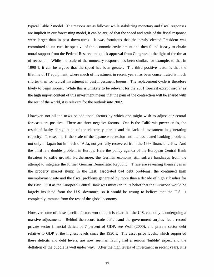
As noted above, another contributing factor to the 1990-91 recession and subdued growth in the
early 1990’s was the aftermath of the commercial property boom and the associated overbuilding in
the late 1980’s. This left low property prices and high vacancy rates into the mid 1990’s and low
rates of gross investment by businesses in buildings for this period. In Figure 5 we display data on
the rate of return in commercial property and the ratio to GDP of investment in non-residential
building. However, by the second half of the 1990’s, this negative factor should have largely
disappeared. Yet, as Figure 2c reveals, the negative effect of the GDEBT*D89 term moderated
only a little in the second half of the 1990’s.
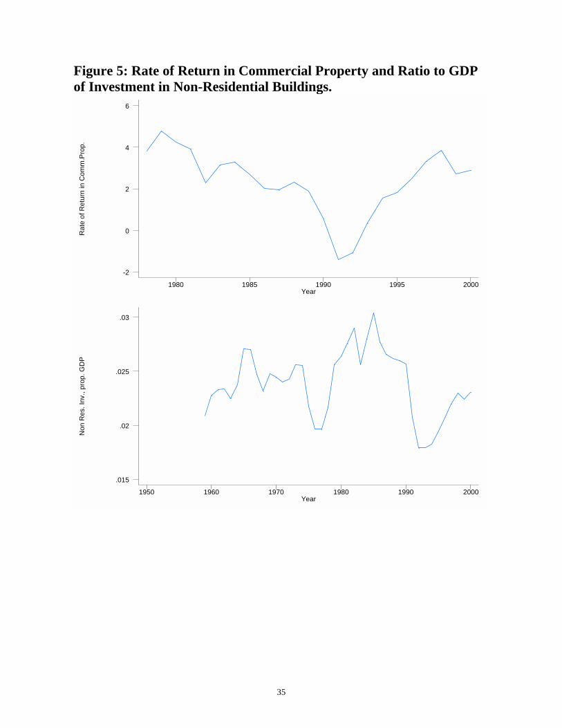
The housing market also suffered what appears to have been the first sustained falls in nominal
prices since the 1950’s. At the broad regional level, the North-East after 1989 and the West after
1991 were the regions in which median house prices fell, while median prices for the Mid-West

17
and the South continued to rise. It seems likely that the experience of negative net housing equity
and higher rates of foreclosure would have dampened both the supply of credit and the willingness
of households to spend, particularly in these regions. A very crude proxy for negative equity can
be obtained by taking the negative deviation from the previous peak median price. Multiply by the
number of units in the affected regions and divide by total US personal disposable income. This
peaks at 9% in 1983, see Figure 6. At one level, this indicator, NEGEQ, overstates negative equity
since it implicitly assumes 100% loan to value ratios for all house owners. One the other hand, the
median house price data disguise local and individual variations and so greatly understate the
prevalence of negative equity. It seems likely that NEGEQ is strongly correlated with the correct
concept.
We have argued that the Table 1 and 2 specifications may be exaggerating the effect of GDEBT89.
We now investigate whether a mixture of calibration and estimation, which makes a rough
allowance for negative equity in the housing market and for high vacancy rates and early scrapping
in the commercial property market, produces plausible results. A simple proxy for the
underutilization and early scrapping of part of the stock of buildings in this period is to assume that
a temporary reduction occurred in the growth rate of underlying capacity. A negative effect from a
split trend, T8995, from 1989 to 1995, i.e. zero up to 1988 and rising from 1 in 1989 to 7 in 1995,
then remaining at 7 could be regarded as a proxy for such an effect. A coefficient of -0.04 on
GDEBT89 seems entirely plausible as a proxy for the shift in fiscal policy, instead of the freely
estimated coefficient, which is three or more times as large. If we impose such value, and include
NEGEQ and T8995 in the Table 1 specification, we obtain the results shown in Table 3. While the
fit is a little worse than Table 1, column 3, the other parameters are quite stable in comparison with
the 1955-88 sample. This model implies a longer drawn-out growth slowdown from 1989 to 1995,
in addition to the assumed effect of the shift in the fiscal policy reaction function on spending.
Another robustness issue concerns the presence of ‘bubble’ elements in the rise in the stock market,
particularly in the second half of the 1990’s. If this had been so, the real stock market index may
have become a less successful predictor of GDP growth. There are two main reasons why the real
S&P index in year t should help explain GDP growth in year t+1. One is that higher stock prices
increase spending: wealthier consumers spend more and firms with access to cheaper finance invest
more. The other is that higher stock prices forecast longer term increases in the growth rate since
they are supposed to represent the discounted present value of future earnings streams of

18
companies. However, in the presence of a financial bubble, this second factor would weaken and
one might then expect a drop in the coefficient on the log real S&P index in the second half of the
1990’s. However, conditional upon the inclusion of GDEBT*D89, nothing in the recursive
estimates in Figure 1 is consistent with this view. As noted above, if we omit GDEBT*D89 and
introduce an I(1) stochastic trend estimated using the Kalman filter, we obtain the estimates shown
in Table 1, column 5. These also show no symptom of a drop in the influence of the stock market
terms. Instead, they suggest a drop in the coefficient on TDEFMA(-1), the trade deficit relative to
GDP, with a compensating rise in the coefficient on LGDPWMA, compared with estimates up to
1988.
There are theoretical reasons why the trade deficit relative to GDP might be imposing less of a
constraint on growth over time. For example, after the break-up of the Bretton Woods international
payments system in 1971 and the move to flexible exchange rates, one might have expected a
reduced role for this constraint. Point estimates of such a shift confirm the direction but the size of
the shift is statistically insignificant. The increased international capital mobility of the 1980’s
could be taken as another reason for such a shift, but the recursive estimates in Figure 1 given no
indication of such an effect. One rather speculative argument for such a shift in the 1990’s
concerns the changes in U.S. corporate financial structures in this period. Holmstrom and Kaplan
(2001) argue that, with the spread of stock options for managers, maximizing share-holder value
received much more emphasis in corporate decision taking. This may have made the U.S. equity
market more attractive to foreign investors so that capital inflows were readily available as the
counterpart to higher trade deficits, but without a depreciation of the Dollar against other
currencies.
A simple test of this hypothesis is to interact TDEFMA(-1) with D89. Added to the Table 1,
column 3 specification, this variable has a coefficient of 0.6 (t=0.9). However, if D89 is also
included in the equation, this coefficient rises to 1.5 (t=2.2), leaving a net coefficient on
TDEFMA(-1) after 1992 of –0.6, a considerable reduction from values close to –2 estimated in
earlier samples. In fact, this specification has current implications very similar to those of the
Table 1, column 6 estimates which include a stochastic level and the same point forecast as Table
1, column 3. Remarkably enough, these specification changes have little implications for the one-
year ahead forecasts: weakening the role of the trade deficit appears not to result in less negative
forecasts.

19
Implications for 2001
The fall in the stock market at the end of 2000, higher oil prices, tighter loan standards, the rise in
interest rates between 1999 and 2000, the high level of the trade deficit, the above trend level of per
capita GDP and the high level of the real exchange rate all have negative implications for growth in
2001. The forecasts for U.S. GDP growth (not per capita) in 2001 were shown in the last row of
Tables 1 to 3 and range from 0 percent to –1.5 percent. A visual impression of the contribution of
each variable to the forecast of –0.6 percent growth from column 3 of Table 1, which is in the
middle of this spread, can be obtained by examining the year 2000 plots of each variable in Figure
2, where each variable is weighted by its coefficient estimate from column 1. To see these more
precisely, we can decompose the reversal of 5.5 percent from 4.9 percent growth in 2000 to our
central forecast of a 0.6 percent decline in GDP in 2001, into the factors shown in Table 4.11
The margin of uncertainty around this forecast of -0.6 percent growth is that growth will fall in the
range +0.4 to –1.6 percent with a 95 percent probability.
Using the unemployment rate as the output gap measure - see the Table 2 results - gives the
forecasts shown in the last row of Table 2. Though the fit of these specifications is marginally
inferior to those in Table 1, which use the deviation from trend of GDP per head, the forecasts are
uniformly less negative by between 0.7 to 0.8 percent.
Pointers for 2002
While our model forecasts only one year ahead, there are nevertheless some implications for 2002.
First, note that the trade deficit-to-GDP ratio only reached its all-time peak in 2000. Its maximum
impact on GDP growth is likely to occur in 2002.12 Second, note that a further drag on the
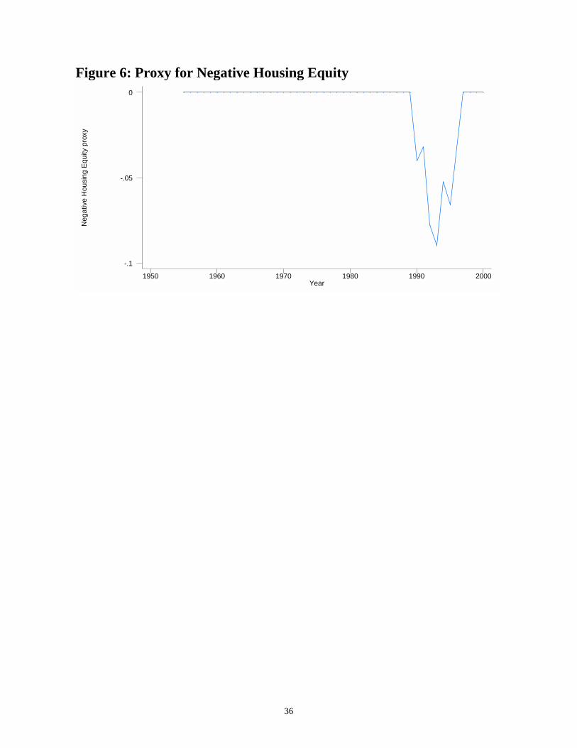
economy in 2002 is almost certain to come from a lower level of real stock prices in 2001. Third,
note that the tightness of loan standards in January 2001 was far worse than the average for 2000,
11 Since the model predicts a 5.2 percent growth rate in 2000 instead of the 4.9% realized, and so a 5.8 percent reversalof predicted rates in 2001, we have scaled the contribution of each estimated factor by 5.5/5.8 to make the figures addto 5.5 percent.

20
though there has been a little improvement in March and May, see Figure 7. It is certainly a
possibility that the annual average of the tightness index in 2001 could be as bad as in 2000.
Finally, little relief has come so far from a fall in the Dollar, probably because of the markets’
perceptions of the policy agenda pursued by the European Central Bank as well as the still fragile
state of banking systems in much of Asia and especially Japan. This suggests that considerable
uplift will have to come from the other factors if positive growth is to be restored in 2002.
Paradoxically, one of these will be a fall in output from its above trend level, but lower real interest
rates and the tax cuts recently passed by Congress will obviously be the key, particularly if they
have a positive enough impact on asset values and credit conditions.
4. Conclusions
Our range of comprehensive forecasting models for annual growth of U.S. GDP encompass most of
the important variables investigated in econometric research in recent years – and more, because
they also incorporate the wider macro context: fiscal policy, the trade balance and the real
exchange rate. The models offer an integrated perspective on the U.S. business cycle since the
mid-1950‘s, illuminating such major questions as the effect of monetary policy, changes in credit
market conditions, the stock market and oil prices on the business cycle. The models offer strong
evidence for the ‘financial accelerator’ or ‘credit channel’ views of monetary policy transmission.
Our estimates also suggest that the Lucas critique is relevant for forecasting U.S. growth: we find
evidence of an important shift in the fiscal policy feedback rule from 1989, consistent with claims
by Muellbauer (1996). Increased concerns by policy makers with the federal government deficit
and debt, appears to have caused an important shift in the effect of the debt on subsequent growth.
However, it is likely that the other factors contributed to the 1990-91 recession and the
sluggishness of the subsequent recovery. Conditional on the index of tighter loan standards, we
find little evidence of a shift in response to the shift in the monetary policy rule around 1980.
However, our investigation of the determinants of this index itself shows clear evidence of a break
around 1980.
12 However, since our discussion has indicated that there is some uncertainty about the current size of the impact of thetrade deficit on the growth forecast, this increases the uncertainty about the outlook for 2002.

21
Whether our comprehensive models exhibit the asymmetries in the business cycle and regime
switches in the stochastic process intensively investigated by Hamilton and others remains to be
investigated on quarterly data. What is clear is that the models offer some fascinating perspectives
on the U.S. economic outlook. For example, the models find little evidence of any speed-up in the
underlying growth rate of the economy in the latter half of the 1990’s, given the real stock market
index, the government debt to GDP ratio and the other variables. One obvious interpretation is that
the recorded improvements in multi-factor productivity growth have been capitalized in the stock
market, the high real exchange rate and perhaps reflected in the decline in the government debt to
GDP ratio. The contribution to growth of the rising stock market and the falling government debt to
GDP ratio in the second half of the 1990’s is notable. However, the fact that demand growth has
outstripped supply is indicated in the trade deficit to GDP ratio. More recently, the fall in the stock
market at the end of 2000, higher oil prices, higher inflation, tighter loan standards, the rise in
interest rates between 1999 and 2000, the high level of the trade deficit, the high level of the output
gap and the high level of the real exchange rate all have negative implications for growth in 2001.
Indeed, our estimated lags suggest that the record trade deficit to GDP ratio is likely to dampen
growth for several years to come.
It is worth spelling out the negative feedback mechanisms operating in the years 2000-2001 via
equity and credit markets. Lower share prices have the effect of reducing consumer spending. The
consensus view is that, in the U.S., 3.5 to 5 cents of every dollar of stock market wealth is spent by
consumers each year, with spending lagging behind share price movements. The longest lags arise
from the part of wealth tied up in pension funds lying outside the direct control of households:
these tend to adjust contribution rates very slowly in response to changes in asset values.
Business investment too is affected by equity prices, since lower equity prices raise the cost of
capital. A sustained fall in share prices, therefore, leads to lower spending and lower income
growth, which in turn, by lowering growth expectations can further lower share prices.
The other key ingredient in the negative feedbacks operating in 2001 is the financial accelerator.
The notion of the ‘financial accelerator’ has been used by economists , see Bernanke et al (1996)
(though the ideas go back, at least, to Irving Fisher, writing in the 1930’s), to describe the process
of credit contraction when asset prices fall. Much of the borrowing from banks and other financial
institutions is backed by collateral, with both the amount of borrowing and credit terms such as

22
interest rates or duration of loans depending on collateral values. When asset prices fall, collateral
backing is reduced, tending to diminish credit availability and raise the effective interest rates at
which finance can be obtained. In the last year, the ‘spreads’ between corporate bond yields and
safe government bond yields have risen sharply, signalling that investors have become more
concerned about corporate default risks and that credit lines from banks have contracted with the
fall in asset values and lower growth expectations. The quarterly U.S. Federal Reserve Senior
Loan Officer Surveys show credit conditions tightening in the U.S. throughout 2000 and into 2001,
see Figure 7. Spending and therefore growth falls with credit contraction, providing an important
aspect of the feedback.
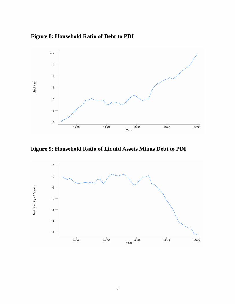
U.S. consumers have a particularly high debt exposure, with household debt to income ratios at the
highest levels and the ratio of liquid assets minus debt to personal disposable income at the lowest
for 70 years, see Figures 8 and 9. Spending has recently exceeded income because asset values
were so high and consumers were confident about future income growth. Many consumers have
been financing part of their spending by increasing borrowing. Indeed, default rates on consumer
credit have been running at historically high levels, even in these years of record growth and low
unemployment. Lower growth and lower collateral values are bound to result in a substantial rise
in default rates from current levels, making banks more wary about lending. Lower share prices of
banks are likely both to signal the rising proportion of bad loans, and, by limiting the capital-raising
opportunities of banks, restrict credit supplies further, see Bernanke and Lown (1991).
In the absence of policy intervention, this analysis points to a downward spiral, such as seen in the
collapse of the ‘bubble economy’ in Japan in the early 1990s and the financial crisis in Thailand in
1997. However, the U.S. Federal Reserve has already lowered the federal funds rate by 2.5
percentage points since January to arrest the process. This appears to be a speedier response than in
the 1990 recession. The U.S. economy is much more sensitive to interest rates than the Japanese.13
Furthermore, fiscal policy has been loosened with exceptional speed. Thus, it is highly improbable
that the U.S. could suffer a decade long recession Japanese style.
Practical forecasters almost always add ‘judgement’ to their forecasts. Indeed, there are some
reasons to think that the U.S. GDP outcome for 2001 is likely to be at the positive end of the 95%
forecast interval, which is 0.4 to –1.6% for the typical Table 1 model and 0.9 to –1.1% for the
13 Research with Keiko Murata on Japanese consumer spending makes this clear.
23
typical Table 2 model. The reasons are as follows: while stabilizing monetary and fiscal responses
are implicit in our forecasting model, it can be argued that the speed and scale of the fiscal response
were larger than in past down-turns. It was fortuitous that the newly elected President was
committed to tax cuts irrespective of the economic environment and then found it easy to obtain
moral support from the Federal Reserve and quick approval from Congress in the light of the threat
of recession. While the scale of the monetary response has been similar, for example, to that in
1990-1, it can be argued that the speed has been greater. The third positive factor is that the
lifetime of IT equipment, where much of investment in recent years has been concentrated is much
shorter than for typical investment in past investment booms. The replacement cycle is therefore
likely to begin sooner. While this is unlikely to be relevant for the 2001 forecast except insofar as
the high import content of this investment means that the pain of the contraction will be shared with
the rest of the world, it is relevant for the outlook into 2002.
However, not all the news or additional factors by which one might wish to adjust our central
forecasts are positive. There are three negative factors. One is the California power crisis, the
result of faulty deregulation of the electricity market and the lack of investment in generating
capacity. The second is the scale of the Japanese recession and the associated banking problems
not only in Japan but in much of Asia, not yet fully recovered from the 1998 financial crisis. And
the third is a double problem in Europe. Here the policy agenda of the European Central Bank
threatens to stifle growth. Furthermore, the German economy still suffers handicaps from the
attempt to integrate the former German Democratic Republic. These are revealing themselves in
the property market slump in the East, associated bad debt problems, the continued high
unemployment rate and the fiscal problems generated by more than a decade of high subsidies for
the East. Just as the European Central Bank was mistaken in its belief that the Eurozone would be
largely insulated from the U.S. downturn, so it would be wrong to believe that the U.S. is
completely immune from the rest of the global economy.
However some of these specific factors work out, it is clear that the U.S. economy is undergoing a
massive adjustment. Behind the record trade deficit and the government surplus lies a record
private sector financial deficit of 7 percent of GDP, see Wolf (2000), and private sector debt
relative to GDP at the highest levels since the 1930’s. The asset price levels, which supported
these deficits and debt levels, are now seen as having had a serious ‘bubble’ aspect and the
deflation of the bubble is well under way. After the high levels of investment in recent years, it is

24
clear that U.S. firms and households will not soon be spending as freely in the new economic
environment. Our models suggest that the scale of the short-term GDP adjustment will be
dramatic despite the swift response of monetary and fiscal policy.

25
Table 1: US Growth Forecasting Models
M 1 M2 M3(1) (2) (3) (4) (5) (6)
55-88 55-95 55-99 55-99 55-88 55-99
LGDPMAW -0.359 -0.368 -0.34 -0.335 -0.359 -0.457[7.3] [8.3] [7.7] [8.0] [7.3] [3.3]
INFLD -0.252 -0.268 -0.287 -0.288 -0.252 -0.241[3.7] [4.6] [4.5] [4.8] [3.7] [2.3]
D. RIR3 -0.444 -0.442 -0.47 -0.507 -0.444 -0.396[5.6] [6.3] [6.6] [7.2] [5.6] [4.6]
L. TDEFMA -2.255 -2.041 -1.926 -2.077 -2.255 -0.739[6.2] [7.5] [7.6] [8.5] [6.2] [1.6]
LSP 0.055 0.061 0.054 0.054 0.055 0.047[5.6] [8.1] [11.0] [11.7] [5.6] [3.2]
TLS -0.03 -0.029 -0.031 -0.031 -0.030 -0.027[2.8] [3.4] [3.3] [3.5] [2.8] [2.3]
LREER -0.062 -0.063 -0.074 -0.062 -0.045[4.3] [4.8] [5.3] [4.3] [1.6]
WHDLQ 0.022 0.021 0.021 0.022 0.022 0.023[6.5] [6.9] [6.5] [7.2] [6.5] [5.8]
D. LSPD 0.07 0.073 0.071 0.069 0.070 0.067[8.2] [9.7] [8.9] [9.1] [8.2] [6.8]
TREND 0.854 0.854 0.786 0.791 0.854 0.801[8.1] [8.8] [7.8] [8.3] [8.1] [2.8]
DV73 -0.025 -0.025 -0.026 -0.02 -0.025 -0.022[4.2] [4.7] [4.6] [3.7] [4.2] [3.2]
DEVOILMA -0.024 -0.018 -0.017 -0.014 -0.024 -0.019[2.4] [2.5] [3.0] [2.6] [2.4] [1.7]
STOVOLMA -0.16 -0.131 -0.264 -0.235 -0.160 -0.154[1.3] [1.3] [2.6] [2.4] [1.3] [1.0]
GDEBT*D89 -0.138 -0.136 -0.16[12.7] [11.6] [11.9]
LREER* -0.004[5.9]
Constant -15.67 -15.66 -14.327 -14.796 Stoch. level Stoch. level[8.0] [8.7] [7.7] [8.4]
Observations 34 41 45 45 34 45Adjusted R-squared 0.9598 0.9599 0.9496 0.9542 0.9861 0.9360
RMSE 0.0048 0.0045 0.0049 0.0047 0.0037 0.0072DW 2.5868 2.4548 2.0343 2.1733 2.4004 1.8230LM 2 .0532 .0239 .1743 .2490
f -0.006 -0.008 -0.010Absolute value of t statistics in bracketsLM 2 refers to p-values of Lagrange multiplier tests for second order residual autocorrelation

26
Table 2: US Growth Forecasting Models with Unemployment Rate
M 4 M5 M6(1) (2) (3) (4) (5) (6)
55-88 55-95 55-99 55-99 55-88 55-99
URMA 0.955 0.851 0.811 0.901 0.955 1.152[5.6] [5.2] [4.9] [5.9] [5.6] [3.1]
INFLD -0.189 -0.245 -0.274 -0.259 -0.189 -0.190[2.3] [3.2] [3.7] [3.7] [2.3] [1.6]
D. RIR3 -0.404 -0.416 -0.476 -0.492 -0.404 -0.401[4.4] [4.9] [6.0] [6.3] [4.4] [4.5]
L. TDEFMA -1.934 -1.762 -1.592 -1.463 -1.934 -0.454[4.8] [4.7] [4.3] [4.2] [4.8] [0.9]
LSP 0.04 0.048 0.053 0.054 0.040 0.047[4.1] [6.1] [9.2] [9.7] [4.1] [3.1]
TLS -0.032 -0.033 -0.037 -0.035 -0.032 -0.029[2.9] [3.2] [3.7] [3.7] [2.9] [2.4]
LREER -0.052 -0.064 -0.074 -0.052 -0.042[2.6] [3.5] [4.2] [2.6] [1.5]
WHDLQ 0.022 0.02 0.02 0.021 0.022 0.022[6.2] [5.7] [5.8] [6.1] [6.2] [5.4]
D. LSPD 0.07 0.075 0.071 0.071 0.070 0.070[7.7] [8.5] [8.2] [8.4] [7.7] [6.7]
TREND 0.084 0.096 0.093 0.06 0.084 -0.125[1.5] [1.8] [1.7] [1.2] [1.5] [0.8]
DV73 -0.024 -0.024 -0.024 -0.02 -0.024 -0.024[3.9] [3.8] [3.8] [3.3] [3.9] [3.5]
DEVOILMA -0.028 -0.016 -0.005 -0.004 -0.028 -0.014[2.1] [1.7] [0.9] [0.6] [2.1] [1.3]
STOVOLMA -0.112 -0.073 -0.118 -0.091 -0.112 -0.067[0.9] [0.6] [1.1] [0.9] [0.9] [0.4]
LFYT -0.173 -0.251 -0.294 -0.213 -0.173 0.018[1.5] [2.9] [3.5] [2.9] [1.5] [0.1]
GDEBT*D89 -0.124 -0.129 -0.132[5.6] [5.9] [6.2]
LREER* -0.004[4.6]
Constant -1.619 -1.816 -1.728 -1.467[1.5] [1.8] [1.7] [1.6]
Observations 34 41 45 45 34 45Adjusted R-squared 0.9555 0.9467 0.9419 0.9454 0.9742 0.8864
RMSE 0.0051 0.0052 0.0052 0.0051 0.0038 0.0072DW 2.5536 2.1673 1.8887 1.973 2.4270 2.0122LM 2 .0625 .0694 .3543 .3543
f 0.001 0.000 -0.002Absolute value of t statistics in bracketsLM 2 refers to p-values of Lagrange multiplier tests for second order residualautocorrelation

27
Table 3: U.S. Growth Forecasting Models with GDEBT*D89coefficient set at –0.04
M 7 M8(1) (2) (3) (4)
55-88 55-95 55-99 55-99LGDPWMA -0.359 -0.342 -0.301 -0.291
[7.3] [6.4] [5.4] [5.1]INFLD -0.252 -0.272 -0.284 -0.275
[3.7] [3.7] [3.6] [3.5]DRIR3 -0.444 -0.439 -0.436 -0.455
[5.6] [5.0] [4.9] [5.0]TDEFMA (-1) -2.255 -1.987 -1.827 -1.986
[6.2] [5.9] [5.3] [5.6]LSP 0.055 0.056 0.047 0.044
[5.6] [6.1] [5.6] [5.3]TLS -0.03 -0.029 -0.031 -0.031
[2.8] [2.7] [2.7] [2.7]LREER -0.062 -0.056 -0.063
[4.3] [3.5] [3.7]WHDLQ 0.022 0.021 0.021 0.022
[6.5] [5.6] [5.2] [5.5]DLSPD 0.07 0.071 0.072 0.071
[8.2] [7.5] [7.2] [7.0]NEGEQR 0.435 0.244 0.312
[3.6] [2.7] [3.2]TREND 0.854 0.795 0.696 0.693
[8.1] [6.7] [5.6] [5.5]DV73 -0.025 -0.024 -0.025 -0.019
[4.2] [3.7] [3.4] [2.7]DEVOILMA -0.024 -0.019 -0.019 -0.018
[2.4] [2.0] [2.2] [2.1]STOVOLMA -0.16 -0.148 -0.279 -0.274
[1.3] [1.1] [2.1] [2.0]T89-T95 -0.512 -0.679 -0.812
[3.0] [4.6] [5.0]GDEBT*D89 -0.04 -0.04 -0.04 -0.04
(fixed) (fixed) (fixed) (fixed)LREER* -0.003
[3.6]Constant -15.67 -14.578 -12.689 -12.946
[8.0] [6.7] [5.5] [5.6]Observations 34 41 45 45
Adjusted R-squared 0.9598 0.9472 0.9406 0.94RMSE 0.0048 0.0055 0.0061 0.0061
DW 2.5868 2.3777 1.7333 1.751LM 2 .0532 .2757 .3202 .4878
F 2001 -0.011 -0.015Absolute value of t statistics in bracketsLM 2 refers to p-values of Lagrange multiplier tests for second order residualautocorrelation

28
Table 4: decomposing the 2000-2001 growth reversal
Factor Contribution (%)Rise in GDP overshoot relative to trend -0.3Rise in the balance of payments deficit/ GDP -1.5Rise in inflation -0.4Fall in last quarter weekly hours of work -1.1Rise in annual real S&P index 0.2Fall in December/annual real S&P index -1.0Rise in real T-bill rate -0.4Tighter loan standards -0.4Higher real oil prices -0.9Higher real exchange rate index -0.2Lower government debt/GDP 0.5Lower stochastic volatility 0.0TOTAL -5.5

29
Figure 1: Recursive Estimations, Table 1 Column 3 Model
1980 1985 1990 1995 2000
0
.25
.5
.75INFLD
1980 1985 1990 1995 2000
-1
-.5
0 D.RIR3
1980 1985 1990 1995 2000
-4
-2
0TDEFMA(-1)
1980 1985 1990 1995 2000
0
.025
.05
.075LSP
1980 1985 1990 1995 2000
-.1
-.05
0
TLS
1980 1985 1990 1995 2000
.01
.02
.03
.04WHDLQ
1980 1985 1990 1995 2000
-.4
-.2
0LGDPWMA
1980 1985 1990 1995 2000
-.2
-.1
0
LREER
1980 1985 1990 1995 2000
0
.1
D.LSPD
1980 1985 1990 1995 2000
-.1
-.05
0DEVOILMA
1980 1985 1990 1995 2000
-1
-.5
0
.5STOVOLMA
1980 1985 1990 1995 2000
-.2
-.1
0GDEBT*D89

30
Figure 2a: Regressors Contribution to the Dependent Variable, Table1 Column 1 Model
DLG
DP
(+1)
Year1960 1970 1980 1990 2000
-.05
0
.05
LGD
PM
A,C
ON
San
dT
RE
ND
Year1960 1970 1980 1990 2000
.22
.24
.26
.28
INF
LD
Year1960 1970 1980 1990 2000
-.02
0
.02
DR
IR
Year1960 1970 1980 1990 2000
-.04
-.02
0
.02
TD
EF
MA
(-1)
Year1960 1970 1980 1990 2000
-.06
-.04
-.02
0
.02

31
Figure 2b: Regressors Contribution to the Dependent Variable, Table1 Column 1 Model
DLG
DP
(+1)
Year1960 1970 1980 1990 2000
-.05
0
.05
LSP
Year1960 1970 1980 1990 2000
.25
.3
.35
.4
TLS
Year1960 1970 1980 1990 2000
-.015
-.01
-.005
0
.005
LRE
ER
Year1960 1970 1980 1990 2000
-.37
-.36
-.35
-.34
-.33
WH
DLQ
Year1960 1970 1980 1990 2000
-.01
0
.01
.02

32
Figure 2c: Regressors Contribution to the Dependent Variable, Table1 Column 1 Model
DLG
DP
(+1)
Year1960 1970 1980 1990 2000
-.05
0
.05
DLS
PD
Year1960 1970 1980 1990 2000
-.01
0
.01
.02
DE
VO
ILM
A
Year1960 1970 1980 1990 2000
-.01
0
.01
.02
ST
OV
OLM
A
Year1960 1970 1980 1990 2000
-.015
-.01
-.005
GD
EB
T*D
89
Year1960 1970 1980 1990 2000
-.1
-.05
0

33
Figure 3: Trend and Stochastic Level, Table 1 Column 3 Model
1955 1960 1965 1970 1975 1980 1985 1990 1995 2000
5.2
5.25
5.3
5.35
5.4
5.45
5.5
5.55
5.6Trend and Stochastic Level

34
Figure 4: Ratios to GDP of Primary Surplus of Federal Governmentand Government debt
Gov
ernm
entS
urpl
us,p
rop.
GD
P
Year1950 1960 1970 1980 1990 2000
-.04
-.02
0
.02
.04
Fed
eral
Deb
t,pr
opor
tion
GD
P
Year1950 1960 1970 1980 1990 2000
.3
.4
.5
.6
.7
35
Figure 5: Rate of Return in Commercial Property and Ratio to GDPof Investment in Non-Residential Buildings.
Rat
eof
Ret
urn
inC
omm
.Pro
p.
Year1980 1985 1990 1995 2000
-2
0
2
4
6
Non
Res
.Inv
.,pr
op.G
DP
Year1950 1960 1970 1980 1990 2000
.015
.02
.025
.03
36
Figure 6: Proxy for Negative Housing EquityN
egat
ive
Hou
sing
Equ
itypr
oxy
Year1950 1960 1970 1980 1990 2000
-.1
-.05
0
37
Figure 7: Measures of Supply and Demand for C&I Loans, by size offirms seeking loans
38
Figure 8: Household Ratio of Debt to PDILi
abili
ties
Year1960 1970 1980 1990 2000
.5
.6
.7
.8
.9
1
1.1
Figure 9: Household Ratio of Liquid Assets Minus Debt to PDI
Net
Liqu
idity
-P
DIr
atio
Year1960 1970 1980 1990 2000
-.4
-.3
-.2
-.1
0
.1
.2

39
REFERENCES
Bernanke, B and A S Blinder, (1992), “The Federal Funds Rate and the Channels of MonetaryTransmission”, Journal of Economic Perspective, 9, 4, 27-48.
Bernanke, B and M Gertler, (1995), “Inside the Black Box: the Credit Channel of Monetary PolicyTransmission”, Journal of Economic Perspectives, vol 9, no 4.
Bernanke, B., M. Gertler and S. Gilchrist. 1996. “The financial accelerator and the flight to
quality.” Review of Economics and Statistics 78 (1): 1-15.
Bernanke, B., M. Gertler and S. Gilchrist. 1999. “The financial accelerator in a quantitative
business cycle framework”, in Handbook of Macroeconomics, ed. J. Taylor and M.
Woodford, New York: North-Holland.
Bernanke, B S and C S Lown, (1991), “The Credit Crunch”, Brookings Papers on EconomicActivity, 0(2), pp. 204-39.
Bernard, H and S Gerlach, (1998), “Does the Term Structure Predict Recessions? The InternationalEvidence”, International Journal of Finance and Economics, 3(3), July, pp. 195-215.
Blanchard, O J, (1993), “Consumption and the Recession of 1990-1991”, American EconomicReview, 83(2), May, pp. 270-74.
Bryant, R C, P Hooper and C L Mann (eds), (1993), Evaluating Policy Regimes: New Research inEmpirical Macroeconomics, Washington DC: Brookings Institution.
Campbell, J Y, (1995), “Some Lessons from the Yield Curve”, Journal of Economic Perspectives,9(3), Summer, pp. 129-52.
Clarida, R, J Gali and M Gertler, (1998), “Monetary Policy Rules in Practice: Some InternationalEvidence”, European Economic Review, 42(6), June, pp. 1033-67.
Clements, M P and H-M Krolzig,(1998), ‘A Comparison of the Forecast Performance of Markov-Switching and Threshold Autoregressive models of US GNP’, Econometrics Journal, 1,C47-C75.
Clements, M P and H-M Krolzig, (2001), “Can oil shocks explain asymmetries in the US BusinessCycle?”, Nuffield College Seminar.
Estrella, A and F S Mishkin, (1998), “Predicting US Recessions: Financial Variables as LeadingIndicators”, Review of Economics and Statistics, 80(1), February, pp. 45-61.
Federal Reserve Bank of Kansas City, (1995), Budget Deficits and Debt: Issues and Options,Symposium at Jackson Hole, Wyoming, September 1995.
Friedman, B and K Kuttner, (1992), “Money, Income, Prices and Interest Rates”, AmericanEconomic Review, 82, 472-492.

40
Gordon, R , (2000) "Does the ‘New Economy’ Measure up to the Great Inventions of the Past?,Journal of Economic Perspectives , Fall, 49-74.
Hall, R E, (1993), “Macro Theory and the Recession of 1990-1991”, American Economic Review,83(2), May, pp. 275-79.
Hamilton, J D, (1983), “Oil and the Macroeconomy since World War II”, Journal of PoliticalEconomy, 91, pp. 228-248.
Hamilton, J D, (1989), “A new approach to the economic analysis of nonstationary time series andthe business cycle”, Econometrica, 57, 357-384.
Hamilton, J D, (1996), “This is what happened to the oil price-macroeconomy relationship”,Journal of Monetary Economics, 38, pp. 215-220.
Hamilton and Lin (1996) bivariate model of stock returns and growth
Hansen, G D and E C Prescott, (1993), “Did Technology Shocks Cause the 1990-1991 Recession?,American Economic Review, 83(2), May, pp. 280-86.
Harvey, Andrew C, (1989), Forecasting, Structural Time Series Models and the Kalman Filter,Cambridge: Cambridge University Press.
Harvey, A and A Jaeger, (1993), “Detrending, Stylized Facts and the Business Cycle”, Journal ofApplied Econometrics, 8, 231-248.
Hans-Martin Krolzig and Juan Toro [1998] “A New Approach to the Analysis of Shocks and theCycle in a Model of Output and Employment”, Discussion Paper, European UniversityInstitute.
Hendry, D F, (1995), Dynamic Econometrics, OUP.
Hendry, D F and Doornik, J A, (1999), Empirical Econometric Modelling Using PcGive (2ndedition), London: Timberlake Consultants Press.
Hendry D F and H-M Krolzig, (1999), “Improving on ‘Data missing reconsidered’, by K DHoover and S J Perez”, Econometrics Journal, 2, pp. 45-58.
Hendry, D F, (2000), Econometrics: Alchemy or Science, Ch. 20, OUP.
Holmstrom, B and S N Kaplan, (2001), “Corporate Governance and Merger Activity in the U.S:Sense of the 1980s and 1990s”, mimeo, M.I.T.
Hooker, M A, (1996), “Whatever happened to the oil price-macroeconomy relationship”, Journalof Monetary Economics, 38, pp. 195-213.
Hoover, K D, and S J Perez, (1999), “Data missing reconsidered: Encompassing and the general-to-specific approach to specification search”, Econometrics Journal, 2, pp.1-25.
Koopman, S J, Harvey, A C, Doornik, J A, and Shephard, N, (2000), Stamp: Structural TimeSeries Analyser, Modeller and Predictor, London: Timberlake Consultants Press.
Lucas, R E, (1976), “Econometric Policy Evaluation: a Critique”, in Brunner K and A H Meltzer,(eds), The Phillips Curve and Labour Markets, North-Holland, Amsterdam.
Mork, K A, (1989), “Oil and Macroeconomy when prices go up and down: An extenstion ofHamilton’s results”, Journal of Political Economy, 97, pp. 740-744.

41
Muellbauer, J, (1996), “Income Persistence and Macropolicy Feedbacks in the US”, OxfordBulletin of Economics and Statistics, 58, pp. 703-733.
Peel, D A and M P Taylor, (1998), “The Slope of the Yield Curve and Real Economic Activity:Tracing the Transmission Mechanism”, Economics Letters, 59(3), June, pp. 353-60.
Raymond, J E and R W Rich, (1997), “Oil and the Macroeconomy: A Markov State-SwitchingApproach”, Journal of Money, Credit and Banking, 29(2), May, pp. 193-213.
Runkle, D E, (1990), “Bad News from a Forecasting Model of the U.S. Economy”, FederalReserve Bank of Minneapolis Quarterly Review, 14(4), Fall, pp. 2-10.
Runkle, D E, (1990), “Bad News from a Forecasting Model of the U.S. Economy”, FederalReserve Bank of Minneapolis Quarterly Review, 14(4), Fall, pp. 2-10.
Runkle, D E, (1991), “A Bleak Outlook for the U.S. Economy”, Federal Reserve Bank ofMinneapolis Quarterly Review, 15(4), Fall, pp. 18-25.
Runkle, D E, (1992), “No Relief in Sight for the U.S. Economy”, Federal Reserve Bank ofMinneapolis Quarterly Review, 16(4), Fall, pp. 13-20.
Shimer, R, (1998), “Why is the U.S. Unemployment Rate So Much Lower?” (1998) in NBERMacroeconomics Annual, ed. by Ben Bernanke and Julio Rotemberg, vol. 13. MIT Press,Cambridge, MA, pp. 11-61.
Sims, C A, (1980), “Macroeconomics and Reality”, Econometrica, vol 48, pp. 1-48.
Sims, C A, (1992), “Interpreting the Macroeconomic Time Series Fact: the Effects of MonetaryPolicy”, European Econometric Review, Vol 36, pp. 975-1000.
Sims, C A, (1996), “Macroeconomics and Methodology”, Journal of Economic Perspective, 10,105-20.
Taylor, J B, (1999), “Monetary Policy Rules”, NBER Conference Report series, Chicago andLondon: University of Chicago Press, pp ix, 447.
Todd, R M, (1990), “Vector Autoregression Evidence in Monetarism: Another Look at theRobustness Debate”, Federal Reserve Bank of Minneapolis Quarterly Review, Spring, pp.19-37.
Walsh, C E, (1993), “What Caused the 1990-1991 Recession?”, Federal Reserve Bank of SanFrancisco Economic Review, 0(2), pp. 33-48.
White, J and A Wildavsky, (1991), The Deficit and the Public Interest, Los Angeles: University ofCalifornia Press.
Wolf, Martin. 2000. “After the crash. Foreign Policy September/October: 46-52.

42
Appendix 1: THE DATA
DEFINITION AND SOURCES
DLGDPAnnual growth rate of U.S. real GDP minus the growth rate of the working age population one yearearlier. GDP from Department of Commerce (Bureau of the Census and Bureau of EconomicAnalysis), working age population from Department of Labor, Bureau of Labor Statistics.
LGDPWMATwo years moving average of log GDP scaled by working age population.
INFLDINFL-{INFL (-1)+ INFL (-2) +INFL (-3) +INFL (-4)}/4, where INFL is ∆ log Consumer PriceIndex from Department of Labor, Bureau of Labor Statistics.
DRIR∆ 3-Month Treasury Bill Rate, from Federal Reserve Board of Governors.
TDEFMATrade Deficit, proportion of GDP, where trade deficit = - balance goods and services, fromDepartment of Commerce (Bureau of the Census and Bureau of Economic Analysis). Two-yearmoving average.
LSPlog (SP/CPI), where SP is Standard and Poor's S&P500 Stock Index, and CPI is Consumer PriceIndex.
TLSTighter Loan Standards Index , annual average of quarterly data from Federal Reserve’s Survey ofSenior Loan Officers (available for the periods 1967:1-1984:1 and 1990:2-2000:3) whose missingvalues have been estimated by authors.
LREERlog Real Effective Exchange Rate, series constructed chaining data on trade-weighted value of theU.S. dollar from Muellbauer (1996) and Board of Governors of the Federal Reserve System(Broad Index).
GDEBT*D89Federal debt (end of period), proportion of GDP, from Department of the Treasury and Office ofManagement and Budget, interacted with the dummy D89. The latter is zero up to 1988, 0.25 in1989, 0.5 in 1990, 0.75 in 1991 and 1 from 1992 onwards.
WHDLQLast quarter value of average weekly hours of production workers in manufacturing minus theannual average value. The hours series is from Department of Labor, Bureau of Labor Statistics.
DLSPD

43
∆ {December value of log real S&P500 - annual average log real S&P500}.
TRENDYear /100.
DEVOILMATwo years moving average of lnOILP-{ lnOILP(-1)+lnOILP(-2) + lnOILP(-3) + lnOILP(-4) +lnOILP (-5) }/5, where OILP is an annual average of a quarterly Real Oil Price Index(1990:1=100), constructed using real oil price data from J.D. Hamilton web site at the University ofCalifornia, San Diego (http://weber.ucsd.edu/~jhamilto/software.htm).
STOVOLMATwo years moving average of annual average of STOVOLQ, that is a quarterly measure ofVolatility in Share Prices taken as the deviation of the log-change in the real share price index fromthe average change in the previous 36 months , i.e.
STOVOLQ= 2p1/36·[-sp{ofaveragequarterly (−37)]}−(−1)∆ sps
sp being monthly log real S&P 500 index.
LFYTProportion of the labour force aged 16-24, from Department of Labor, Bureau of Labor Statistics.
LREER*Deviation of LREER from its 1965 value, interacted with a split trend which is zero up to 1965 andincreasing by one every following year.
DV73Dummy variable equal to 1 in 1973, zero otherwise.
SUMMARY STATISTICS
Variable Obs Mean Std. Dev. Min MaxDLGDWAP 45 0.02 0.02 -0.03 0.06LGDPWMA 46 3.33 0.26 2.87 3.79INFLD 46 0 0.02 -0.07 0.06DRIR 46 0 0.01 -0.04 0.05TDEFMA 46 0.01 0.01 -0.01 0.03LSP 46 5.73 0.44 5.09 6.98TLS 46 0.09 0.13 -0.19 0.48LREER 46 4.75 0.12 4.52 4.97GDEBT*D89 46 0.14 0.26 0 0.67WHDLQ 46 0.34 0.3 -0.48 0.88DLSPD 46 -0.01 0.11 -0.17 0.27TREND 46 19.77 0.13 19.55 20DEVOILMA 46 -0.09 0.3 -0.94 0.49STOVOLMA 46 0.04 0.01 0.02 0.06LREER* 46 -2.4 3.34 -9.94 2.32

44
Appendix 2: THE AUXILIARY TLS REGRESSION
The Federal Reserve publishes a quarterly survey of Senior Loan Officers at the 80 or so main banks lending to U.S.commercial and industrial companies. There are three main questions which have been asked throughout. The firstasks whether loan standards or credit terms have tightened over the previous three months. The second asks whetherspreads between rates charged and the cost of funds has widened over the same period. And the third asks whetherdemand for loans from commercial and industrial companies has risen in the last three months. The survey resultsreporting the percentages of respondents replying 'yes' to these questions from 1990 to February 2001 are shown inFigure A1. We concentrate on the first question. Thus, we have quarterly data on Net Percentage of Senior LoanOfficers reporting tighter loan standards, from now on TLS. The series stems only from 1967:1 to 2000:3, with missingvalues from 1984:1 to 1990:2 (included). We perform an auxiliary regression of TLS on a set of interest rates and otherfinancial variables in order to estimate the missing values in the series both pre-1967 and between 1984-1990. Fromoriginal monthly data, we calculate the following quarterly series that we use in the auxiliary regression:
1. raaaq: Moody's Seasoned Aaa Corporate Bond Yield, Averages of Business Days, Percent, from Moody's InvestorsService;2. rbaaq: Moody's Seasoned Baa Corporate Bond Yield, Averages of Business Days, Percent, from Moody's InvestorsService;3. ir3fedq: 3-Month Treasury Bill Rate, Secondary Market, Averages of Business Days, Discount Basis, Percent,Source: H.15 Release -- Federal Reserve Board of Governors;4. spq: S&P 500 index, close values;5. rtcm1q: 1-Year Treasury Constant Maturity Rate, Averages of Business Days, Percent, from H.15 Release --Federal Reserve Board of Governors;6. r10tq: 10-Year Treasury Constant Maturity Rate, Percent, from H.15 Release -- Federal Reserve Board ofGovernors;7. cpi: Consumer Price Index, for All Urban Consumers, All Items, 1982-84=100, from U.S. Department of Labor,Bureau of Labor Statistics.8. infl: Inflation Rate, in annual terms, with infl=∆ln(cpi)·400;9. stovolq: Volatility in Share Prices taken as the deviation of the log-change in the real share price index from theaverage change in the previous 36 months , with
stovolq= 2p1/36·[-sp{ofaveragequarterly (−37)]}−(−1)∆ spssp being monthly log real S&P 500 index;
10. spread: Spread between Baa Corporate Bond Yield and 10-Year Treasury Constant Maturity Rate, i.e.spread=rbaaq-r10tq;11. spreada: Spread between Aaa Corporate Bond Yield and 10-Year Treasury Constant Maturity Rate, i.e.spreada=raaaq-r10tq;12. rrtcm: Real 1-Year Treasury Constant Maturity Rate, i.e. rrtcm=rtcm1q-Linfl, where inflation is lagged one quarterto account for lags in agents information about price changes.
We follow a modelling procedure from general to specific, and estimate the following equation over the whole sampleand over pre-1980Q1 and post 1980Q1 sub-samples:
tls(t)= 0β + 1β tls(t-1)+ 2β spreada(t)+ 3β spreada(t-1)+ 4β rrtcm(t)+
+ 5β (∆spq) (t-1)+ 6β stovolq(t)+ 7β stovolq(t-1)+
+ 8β spread(t)+ 9β spread(t-1)+ 10β ∆ir3fedq(t)+ 11β ∆rtcm1q(t)
In order to test for structural breaks due to likely changes in monetary policy regimes, we perform a Chow test,splitting the sample in the two subperiods 1967:1-1979:4 and 1980:1-2000:3. The test statistics F(11,86)=7.06, with P-value ≅ 0.00, rejects the null hypothesis of homogeneous coefficients along the whole sample period. We thereforeestimate two different parsimonious models over the two subsamples:
MODEL 1, 1967:1-1979:4

45
tls(t)= 0α + 1α tls(t-1)+ 2α spread(t)+ 3α spread(t-1)+ 4α ∆ir3fedq(t)+ 5α ∆rtcm1q(t)+ 6α (∆spq) (t-1)
MODEL 2, 1980:1-2000:3
tls(t)= 0δ + 1δ tls(t-1)+ 2δ spreada(t)+ 3δ spreada(t-1) + 4δ rrtcm(t) + 5δ (∆spq) (t-1) + 6δ stovolq(t-1)
The estimations are presented in Table A1, while Figure A2 shows the TLS quarterly series containing the estimatedvalues for the missing gaps. It is interesting to notice that in the first period the relevant spread regressor is calculatedusing rbaa while in the second period it is raaa that seems to matter. From both specifications we note a positive∆spread effect on TLS, possibly reinforced in the second period by a level effect of current spread. Moreoverincreasing stock prices lower TLS in both periods, while the volatility in stock prices has a positive significant effect inthe second period only. Finally, we have a positive significant effect of the yield gap between the 1-Year TreasuryConstant Maturity Rate and the 3-Month Treasury Bill Rate in the first period. This effect is not confirmed in thesecond period, where the real 1-Year Treasury Constant Maturity Rate has instead a positive significant impact intightening loan standards.
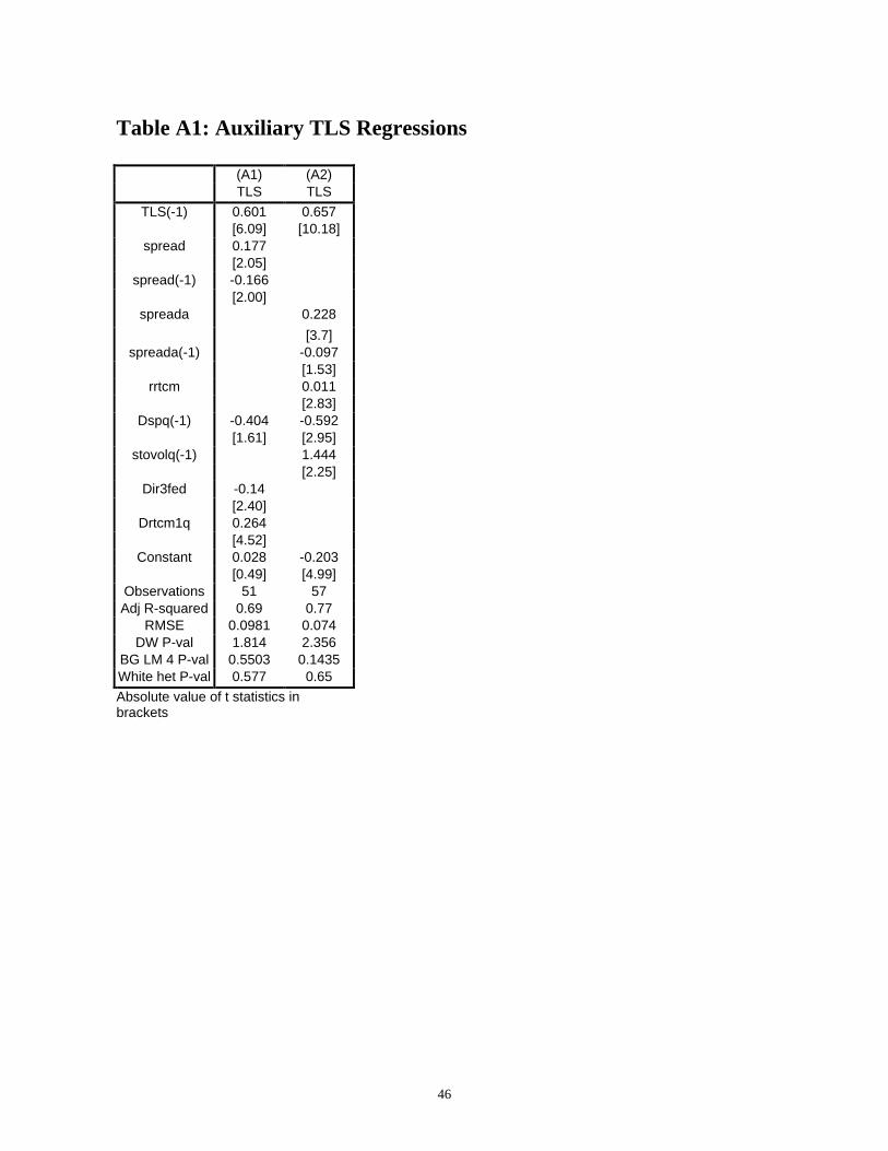
46
Table A1: Auxiliary TLS Regressions
(A1) (A2)TLS TLS
TLS(-1) 0.601 0.657[6.09] [10.18]
spread 0.177[2.05]
spread(-1) -0.166[2.00]
spreada 0.228
[3.7]spreada(-1) -0.097
[1.53]rrtcm 0.011
[2.83]Dspq(-1) -0.404 -0.592
[1.61] [2.95]stovolq(-1) 1.444
[2.25]Dir3fed -0.14
[2.40]Drtcm1q 0.264
[4.52]Constant 0.028 -0.203
[0.49] [4.99]Observations 51 57Adj R-squared 0.69 0.77
RMSE 0.0981 0.074DW P-val 1.814 2.356
BG LM 4 P-val 0.5503 0.1435White het P-val 0.577 0.65
Absolute value of t statistics inbrackets

47
Figure A1: Estimated Quarterly TLS series
Year, Quarter
TLS quarterly actual values TLS quarterly fitted values
1953.25 2000.5
.308333
.766129
Top Related