


Languages
Pages
Legal


Alma Mater Studiorum – Università di Bologna
_____________________________________________________
Use of the Molecular Beam Mass
Spectrometry to study the low-
temperature combustion chemistry
Tesi di Laurea Sperimentale
CANDIDATO
Andrea Secco
RELATORE
Prof. Elisabetta Canè
CORRELATORE
Prof. S. Mani Sarathy
_____________________________________________________
Anno Accademico 2016-2017
SCUOLA DI SCIENZE
Dipartimento di Chimica Industriale “Toso Montanari”
Corso di Laurea Magistrale in
Chimica Industriale
Classe LM-71 - Scienze e Tecnologie della Chimica Industriale

2

3
Table of Content
1. INTRODUCTION .................................................................................................. 13
1.1. Combustion principles ............................................................................................... 16
1.1.1. Combustion reactions ............................................................................................ 18
1.1.2. Low-temperature gas phase fuel oxidation .......................................................... 20
1.2. Mass Spectrometry ..................................................................................................... 24
1.2.1. The inlet system ...................................................................................................... 28
1.2.2. Ionization Source .................................................................................................... 29
1.2.3. Mass Analyser......................................................................................................... 31
1.2.3.1. Time-of-flight .......................................................................................................... 31
1.2.3.2. Setup of the TOF analyser ..................................................................................... 33
1.2.3.3. Detector ................................................................................................................... 36
1.2.3.4. Electron multiplier (EM) detector ........................................................................ 37
1.2.4. Data Output ............................................................................................................ 38
1.3. Research objectives .................................................................................................... 39
2. METHODOLOGY ................................................................................................. 41
2.1 Experimental apparatus specification ...................................................................... 41
2.1.1. Propane oxidation .................................................................................................. 41
2.1.2. Cool flame in counterflow setup ........................................................................... 44
2.2. Safety consideration ................................................................................................... 46
2.3. Data analysis ............................................................................................................... 47
3. RESULTS AND DISCUSSION ............................................................................. 52
3.1 Propane oxidation ....................................................................................................... 52
3.2. Cool flame structure ................................................................................................... 65
3.2.1. Propane flame ......................................................................................................... 66
3.2.2. N-butane flame ....................................................................................................... 68
4. CONCLUSION ....................................................................................................... 72
5. BIBLIOGRAPHY ................................................................................................... 74

4
5
Table of Figures
Figure 1 Top ten emitting countries in 2014 [3]. .............................................................. 13
Figure 2 Representations of SI, Diesel and HCCI engines. Figure taken from J.P.
Angelos, W.H. Green and M.A. Singer. ................................................................... 15
Figure 3 Reaction mechanism of the low-temperature oxidation for alkanes [16]. ......... 21
Figure 4 Reactions between alkyl radical and molecular oxygen [16]. ............................ 23
Figure 5 Aston's mass spectrograph [20]. ......................................................................... 24
Figure 6 Dempster's mass spectrometer [20]. ................................................................... 25
Figure 7 Block scheme of a mass spectrometer ................................................................ 27
Figure 8 Regions under vacuum [25]. .............................................................................. 28
Figure 9 Delayed pulse extraction .................................................................................... 33
Figure 10 Illustration of an electrostatic ion mirror or reflectron [35]. ............................ 34
Figure 11 Examples of electron multipliers [36]. ............................................................. 37
Figure 12 Mass spectrum. ................................................................................................. 39
Figure 13 Schematic diagram of experimental apparatus used for propane oxidation. .... 41
Figure 14 Conceptual design of the time-of-flight mass spectrometer at the Clean
Combustion Research Center, KAUST. ................................................................... 42
Figure 15 Picture of time-of-flight mass spectrometer at the Clean Combustion Research
Center, KAUST. ....................................................................................................... 42
Figure 16 Schematic diagram of counterflow system. ..................................................... 45
Figure 17 Picture of the sampling of cool flame. ............................................................. 46
Figure 18 Detail of the probe inside the cool flame during the sampling. ....................... 46
Figure 19 Spectrum obtained with no reaction. ................................................................ 48
Figure 20 Spectrum obtained during the reaction. ............................................................ 49
Figure 21 Comparison between data taken with TOF-MBMS (blue dots) and numerical
simulation (red line) for propane. ............................................................................. 52
Figure 22 Comparison between data taken with TOF-MBMS (blue dots) and numerical
simulation (red line) for oxygen. .............................................................................. 53
Figure 23 Comparison between data taken with TOF-MBMS (blue dots) and numerical
simulation (red line) for carbon dioxide. .................................................................. 54
Figure 24 Comparison between data taken with TOF-MBMS (blue dots) and numerical
simulation (red line) for carbon monoxide. .............................................................. 54

6
Figure 25 Comparison between data taken with TOF-MBMS (blue dots) and numerical
simulation (red line) for propylene............................................................................55
Figure 26 Comparison between data taken with TOF-MBMS (blue dots) and numerical
simulation (red line) for allyl radical.........................................................................56
Figure 27 Comparison between data taken with the TOF-MBMS (blue dots) and
numerical simulation (red line) for ethylene. ............................................................57
Figure 28 Comparison between data taken with the TOF-MBMS (blue dots) and
numerical simulation (red line) for methane. ............................................................57
Figure 29 Comparison between data taken with the TOF-MBMS (blue dots) and
numerical simulation (red line) for acetylene. ..........................................................58
Figure 30 Comparison between data taken with the TOF-MBMS (blue dots) and
numerical simulation (red line) for formaldehyde. ...................................................58
Figure 31 Comparison between data taken with the TOF-MBMS (blue dots), GC (green
line) and numerical simulation (red line) for propane...............................................60
Figure 32 Comparison between data taken with the MBMS (blue dots), GC (green line)
and numerical simulation (red line) for oxygen. .......................................................60
Figure 33 Comparison between data taken with the MBMS (blue dots), GC (green line)
and numerical simulation (red line) for carbon monoxide. .......................................61
Figure 34 Comparison between data taken with the MBMS (blue dots), GC (green line)
and numerical simulation (red line) for carbon dioxide. ...........................................62
Figure 35 Comparison between data taken with the MBMS (blue dots), GC (green line)
and numerical simulation (red line) for propylene. ...................................................62
Figure 36 Comparison between data taken with the MBMS (blue dots), GC (green line)
and numerical simulation (red line) for ethylene. .....................................................63
Figure 37 Comparison between data taken with the MBMS (blue dots), GC (green line)
and numerical simulation (red line) for methane. .....................................................64
Figure 38 Comparison between data taken with the MBMS (blue dots), GC (green line)
and numerical simulation (red line) for acetylene. ....................................................64
Figure 39 Experimental measurements of the structure of propane cool flame at strain
rate 44 s-1 and 5.94% ozone addition. .......................................................................67
Figure 40 Numerical simulation of the structure of propane cool flame at strain rate 44 s-1
and 5.94% ozone addition. ........................................................................................67

7
Figure 41 Experimental measurements of the structure of propane cool flame at strain
rate 44 s-1 and 5.94% ozone addition. ....................................................................... 68
Figure 42 Numerical simulation of the structure of propane cool flame at strain rate 44 s-1
and 5.94% ozone addition. ........................................................................................ 68
Figure 43 Experimental measurements of the structure of n-butane cool flame at strain
rate 61 s-1 and 5.02% ozone addition. ....................................................................... 69
Figure 44 Numerical simulation of the structure of n-butane cool flame at strain rate 61 s-
1 and 5.02% ozone addition. ..................................................................................... 69
Figure 45 Experimental measurements of the structure of n-butane cool flame at strain
rate 61 s-1 and 5.02% ozone addition. ....................................................................... 70
Figure 46 Numerical simulation of the structure of n-butane cool flame at strain rate 61 s-
1 and 5.02% ozone addition. ..................................................................................... 70
Figure 47 Numerical simulation structure of propane cool flame with temperature profile
at strain rate 44 s-1 and 5.94% ozone addition. ......................................................... 71
Figure 48 Numerical simulation structure of n-butane cool flame with temperature profile
at strain rate 61 s-1 and 5.02% ozone addition. ........................................................ 71

8

9
Abstract
With the aim to reduce the global pollution caused by the increasing levels of NOx, CO
and the greenhouse gas CO2 emitted by internal combustion engines, the study of low-
temperature chemistry (LTC) of the combustion process has been greatly enhanced.
Numerous efforts are devoted to the development of more efficient engines with lower
emissions such as the homogeneous charge compression ignition engines (HCCI). So, a
deeper knowledge of the chemistry and physics of the oxidation reactions at low
temperature is strongly pursued.
The goal of this thesis work is to evaluate the performances of the time-of-flight
Molecular Beam Mass Spectrometry (TOF-MBMS) in the analysis of the oxidation of
propane at low temperature with strong interest in the detection of fleeting species to
verify the low-temperature oxidation mechanism. To do that we performed two different
experiments: propane oxidation in jet stirred reactor and ozone activated cool diffusion
flame in a counterflow setup. The first was carried out flowing a mixture of C3H8/O2/Ar
with molar fraction 2/13/85%, respectively, corresponding to a 𝜙 equals to 0.77, in the
temperature range 750-1100 K and residence time τ=1 s. To support the molar fraction
values of the gas mixture from MBMS we analyzed the propane oxidation in the same
conditions with the gas chromatograph (GC) technique. The results have been compared
with the MBMS ones showing good agreement for most of the analysed species.
Numerical simulations of the molar fraction of all species were performed and compared
with experimental data. The results indicate that the model well predicts the trends of the
stable species, except for C2H2. Contrary, the allyl radical molar fraction is overestimated
in experimental results: this could be due to the contribution of propylene fragmentation.
Moreover, the onset of the reaction is predicted by the model at a lower temperature than
in the experiment. This discrepancy suggests an inadequacy of the kinetic model built for
n-heptane.
In cool flame experiments the fuel/N2 and O2/O3 streams are facing each other and both
propane and n-butane were used as fuel. In propane experiments a 50/50% C3H8/N2
mixture has been used with O2 flow rate of 5 dm3/min, which corresponds to an ozone
concentration of 5.94%. For n-butane tests the mixture used was 45/55% for C4H10/N2,
O2 flow rate 7 dm3/min and ozone concentration of 5.02%. The distance between the two

10
burners was 15 mm with both fuels, corresponding to a strain rate of 44 s -1 and 61 s-1 for
propane and n-butane, respectively. Numerical analysis was performed showing a good
prediction of flame position and species profiles through the reaction zone.
L’aumento dell’inquinamento globale dovuto alle emissioni di NOx, CO e di gas serra
come la CO2, sono riconducibili al continuo incremento dell’utilizzo di mezzi di
trasporto dotati di motori a combustione interna. La ricerca scientifica e applicata
lavorano assiduamente per progettare dispositivi più efficienti e meno inquinanti quali i
motori ad accensione spontanea (homogeneous charge compression ignition engine,
HCCI). Per lo sviluppo di tali dispositivi è necessario lo studio approfondito della
combustione a bassa temperatura.
Lo scopo di questa tesi è quello di verificare le prestazioni della spettrometria di massa di
fasci molecolari con tempo di volo (time-of-flight Molecular Beam Mass Spectrometry,
TOF-MBMS) nell’ analisi qualitativa e quantitativa delle specie chimiche coinvolte nella
combustione del propano e del n-butano a bassa temperatura. L’analisi con la
spettrometria di massa dei gas in uscita dal reattore è potenziata nel MBMS perchè la
trasformazione in fascio molecolare dei gas prodotti congela la miscela permettendo di
individuare anche le specie labili. Questa informazione è preziosa al fine di comprendere
meglio il meccanismo di reazione. La scelta del propano e del butano come combustibili
è dipesa dalla semplicità di queste molecole caratterizzate da spettri di massa con un
numero limitato di frammentazioni agevolando l’interpretazione degli spettri di massa
ottenuti. Sono stati realizzati due tipi di esperimenti: nel primo abbiamo studiato
l’ossidazione del propano tra 750 e 1100 K, con un tempo di contatto τ = 1 s e frazioni
molari della miscela di gas in entrata pari a 2/13/85% rispettivamente per C3H8/O2/Ar, a
cui corrisponde un rapporto di combustibile e ossigeno 𝜙 pari a 0.77. A conferma delle
misure con il TOF-MBMS abbiamo ripetuto l’esperimento nelle stesse condizioni,
analizzando le specie in uscita con il gas cromatografo. Il confronto dei dati ottenuti dai
due strumenti ha confermato l’adeguatezza e le potenzialità della spettrometria di massa
di fasci molecolari. Inoltre, sono state condotte simulazioni numeriche dell’ossidazione
del propano ottenendo un buon accordo tra gli andamenti sperimentali e calcolati delle
frazioni molari di reagenti e prodotti stabili in funzione della temperatura. Invece la

11
simulazione della specie labile radicale allilico differisce molto dai risultati sperimentali.
Questa differenza potrebbe dipendere dal tipo di modello cinetico usato nella
simulazione, modello pensato e costruito per il n-eptano.
L’altra serie di esperimenti mira allo studio della struttura di una fiamma piatta a bassa
temperatura accesa grazie alla presenza di ozono. Come combustibili sono stati usati
propano e n-butano. Nella combustione del propano la miscela di C3H8/N2 era al 50%
mentre la miscela ossidante era composta da un flusso di O2 = 5 dm3/min e
concentrazione di ozono pari al 5.94%. Per il butano la miscela utilizzata era 45/55%
C4H10/N2, mentre il flusso di O2 era impostato a 7 dm3/min con conseguente
concentrazione di ozono del 5.02%. Per entrambe le prove la distanza tra i due ugelli è
stata fissata a 15 mm. Dati i parametri utilizzati è stata calcolata una velocità di
deformazione della fiamma piatta pari a 44 s-1 per il propano e 61 s-1 per il n-butano.
Anche in questo caso sono state effettuate simulazioni numeriche che hanno mostrato
una buona previsione della posizione della fiamma rispetto agli ugelli del combustibile e
dell’ossigeno e un’ accettabile riproduzione dei profili di concentrazione di reagenti e
prodotti.

12

13
1. INTRODUCTION
Almost the total of the energy demand (~80%) is provided by combustion of gasoline,
wood, coal or hydrocarbons such as ethane, propane, butanes and pentanes [1]. The
European June 2017 Report on energy statistics [2] indicates that the energy
consumption in Europe that derives from petroleum and its products is 429.6 Mtoe
(37%). However only two European countries, Germany and Russia, are among the most
polluting countries in the world, as shown in Figure 1; China and Unites States are
leading this ranking with 28% and 16% [3] of global emissions, respectively. Day after
day the research of a more sustainable way of energy production and the concern about
the climate change are leading to the use of renewable sources of energy. Even if the use
of fossil fuels is decreasing, the process which leads to a less polluted world will take
time. The level of CO2 in 2015 (399 ppm) was 40% higher than in mid-1800s and it has
grown on average at the rate of 2 ppm per year only in the last decade [3]. Especially the
transportation sector is dominated by the use of fossil fuels for internal combustion
engines, which are the major contributors of pollutants, oxides of nitrogen (NOx), carbon
monoxide (CO) and greenhouse gases such as CO2 [4]. In the internal combustion
engine, which is in use for marine, air, rail and road transports, the reaction between fuel
and oxidizer takes place in a combustion chamber where the production of gaseous
products at high temperature and pressure push some components of the engine. In this
Figure 1 Top ten emitting countries in 2014 [3].

14
way, the chemical energy is converted into mechanical energy so the vehicle moves.
There are two conventional types of combustion engines: spark-ignition (SI) and
compression ignition (CI). The SI engines work with gasoline refined from petroleum
crude oil, and fuel and air are mixed together in the intake system before entering in the
engine cylinder. Then a compression occurs and the combustible is initiated by a spark
but, since these engines work with low compression ratio, the efficiency is low [5]. The
CI engines, also known as diesel engines, have higher efficiency thanks to a high
compression ratio. In the typical setup first air is introduced into the combustion
chamber, it is compressed so the temperature rises. The fuel is added in the form of small
droplets to achieve a uniform distribution in the chamber. Being the chamber at high
temperature the fuel evaporates, ignites and burns without any sparks [6].
The efficiency in SI engine could be improved increasing the compression ratio.
However, this could lead to an engine knock, which is an abnormal combustion
phenomenon where a small portion of the mixture fuel-air and residual gases
spontaneously ignite before being reached by the flame front. This occurs because while
the flame propagates inside the combustion chamber, pressure and temperature increase
so the residual gaseous fuel-air mixture may undergo reaction [5, 7].
Since the internal combustion engines emit several pollutants, as evidenced by Hansen et
al. [4], year after year new and always more restrictive emissions regulations must be
respected by car manufacturers. The available SI engines with 3-way catalyst are able to
reduce urban pollutants emissions, while diesel engines are more effective at reducing
CO2 emissions [8].
The truly valid alternative which combines the reduction of pollutant emissions and high
efficiency in the conversion of chemical to mechanical energy is a new concept of
engine. The homogeneous charge compression ignition (HCCI) engine is an example of
this new technology: it is a low-temperature combustion (LTC) device and combines
both spark ignition and diesel engine principles. It works with premixed inlet as in the
spark ignition, and with a lean fuel-air ratio, low temperature and relatively high pressure
as in the diesel engine, parameters which leads combustion only on compression ignition.
The combination of the two traditional engines is pursued to achieve an optimal system
which works with diesel-like efficiency and low emission of NOx, thanks to the low-
temperature combustion. However, the application of these parameters leads to emissions

15
of larger quantities of carbon monoxide (CO) and unburned hydrocarbons due to the
incomplete combustion [9]. The HCCI engines work with a premixed inlet and a lean,
homogeneous fuel-air mixture ratio; the ignition occurs due only to compression and the
chemical kinetics control the heat release rates [7, 8]. In Figure 2 the main differences
between actual models and new concept of engines now under study are shown.
Figure 2 Representations of SI, Diesel and HCCI engines. Figure taken from J.P. Angelos, W.H. Green
and M.A. Singer.
The characteristics of spark ignited, Diesel and HCCI engines are summarized in Table
1.

16
Table 1 Comparison between SI, Diesel and HCCI engines characteristics [8].
However, the improvements described above are not enough and a further development
of these engines is necessary. To this aim it is essential a very good knowledge for both
combustion at high and low temperature. To better understand the combustion is
necessary a deep knowledge of different scientific disciplines such as chemical kinetics,
fluid dynamics and thermodynamics [10]. The actual main goals of the study of
combustion are the pursuit of more efficiency for energy transformation, the reduction of
emissions and the improvement in safety [11].
1.1. Combustion principles
The combustion is a fast, gas phase radical reaction which occurs when fuel (e.g.
gasoline, methane, ethanol) and oxidizer (oxygen) react to mainly produce heat, carbon
dioxide and water.
An important factor that provides useful information about the reaction is the fuel-to-
oxidizer ratio, called equivalence ratio, 𝜙:
𝜙 =(𝑚𝑓𝑢𝑒𝑙 𝑚𝑜𝑥)⁄
𝑎𝑐𝑡
(𝑚𝑓𝑢𝑒𝑙 𝑚𝑜𝑥)⁄𝑠𝑡
=(𝑛𝑓𝑢𝑒𝑙 𝑛𝑜𝑥)⁄
𝑎𝑐𝑡
(𝑛𝑓𝑢𝑒𝑙 𝑛𝑜𝑥)⁄𝑠𝑡
( 1 )
where 𝑚 is the mass, 𝑛 represents the number of the moles, the subscript 𝑠𝑡 indicates the
stoichiometric conditions and 𝑎𝑐𝑡 the actual mixture. When the value of 𝜙 is equal to 1
the mixture is stoichiometric; for 𝜙 < 1 and 𝜙 > 1 we have a fuel-lean and a fuel-rich
Spark ignited Diesel HCCI
Fuel-air mixture Premixed Non-premixed Premixed
Ignition type Spark ignited Compression ignited Compression ignited
Mechanism controlling fuel
burning rate
Flame propagation
speed
Time for fuel
vaporisation and
mixing
Chemical kinetics
Emissions characteristics
Cleaner with 3-way
catalyst. Higher
CO2.
Higher particulate
matter, soot, NOx;
lower CO2.
Higher unburned
hydrocarbons and CO.
Lower NOx, soot,
particulates, and CO2.

17
condition, respectively. In the stoichiometric conditions there is just enough oxidizer to
react with all the fuel present in the system. The general stoichiometric relation for
combustion of a generic non-oxygenated hydrocarbon in the air is:
𝐶𝑥𝐻𝑦 + 𝜉(𝑂2 + 3.76𝑁2) → 𝑥𝐶𝑂2 + (𝑦
2) 𝐻2𝑂 + 3.76𝜉𝑁2
( 2 )
with 𝜉 = 𝑥 +𝑦
4 [11].
The rH is the variation of enthalpy as a result of a chemical reaction. A reaction is
exothermic when releases heat and the value of rH is negative; otherwise the reaction
absorbs heat and the variation of enthalpy is positive (endothermic). This way of
considering rH positive or negative comes from the following convention: the energy
which is coming out of the system is considered negative and the one coming in is
positive.
For a generic reaction between two reagents A and B which give C and D as products,
with a, b, c and d as stoichiometric coefficients
𝑎𝐴 + 𝑏𝐵 ⟶ 𝑐𝐶 + 𝑑𝐷
( 3 )
it is possible to write an equally generic formula for the rH of reaction:
𝛥𝑟𝐻 = ∑ 𝜈𝐽
𝐽
𝐻𝑇(𝐽)
( 4 )
where νJ is the stoichiometric coefficient (a, b, c and d) for the species J (A, B, C and D),
which is negative for reagents and positive for products; 𝐻𝑇(𝐽) is the molar enthalpy for
the species J at temperature T.
According to the Hess law the change of enthalpy for a reaction does not depend on the
pathway. Therefore, it is possible to calculate the ΔrH of a given reaction combining the
ΔrH of known reactions into which the former one can be divided [10].

18
1.1.1. Combustion reactions
Generally speaking, the most reactive species in a reaction are atoms (H, O, N and Cl) or
molecules (CH3, OH and CH) defined as radicals. The radical species have unpaired
electrons and they can be neutral or charged [1].
Combustion reactions are defined as chain reactions, which means that the reagents of a
given reaction are the products of a previous one. The reactions consist in several
consecutive reaction steps with different reaction rate constants. Specifically, the
reactions included in combustion process can be classified in four different groups.
1. Initiation reactions
𝑓𝑢𝑒𝑙 + 𝑂2 ⟶ 𝑓𝑢𝑒𝑙 𝑟𝑎𝑑𝑖𝑐𝑎𝑙 + 𝐻𝑂2
( 5 )
𝑓𝑢𝑒𝑙 + 𝑋 ⟶ 𝑓𝑢𝑒𝑙 𝑟𝑎𝑑𝑖𝑐𝑎𝑙 + 𝑋𝐻
( 6 )
where X represents the radical pool which includes radicals such as OH, H, O,
HO2. These reactions begin the combustion: the interaction between the fuel and
the molecular oxygen produces the radicals which are fundamental for
combustion because they initiate several reactions.
2. Chain branching reactions. These allow the population of the radical pool to
grow.
𝐻⦁ + 𝑂2 ⟶ ⦁𝑂𝐻 + 𝑂⦁
( 7 )
The reaction (7) describes one of the most important step among the chain-
branching ones; indeed, the radical species ⦁ OH is very reactive and helps to
decrease the ignition delay time.
3. Chain propagation reactions. These do not affect the number of radicals but the
type of radicals. An example of these reactions is given below:

19
𝐻⦁ + 𝐻2𝑂 ⟶ 𝐻2 + ⦁𝑂𝐻
( 8 )
4. Three body reactions. They are also known as chain terminating reactions. Since
they are highly exothermic and the energy barrier is low, a third molecule (M) is
needed to collect the excess of energy, otherwise it will dissociate the product
species into the reactant radicals [10].
𝐻⦁ + ⦁𝑂𝐻 + 𝑀 ⟶ 𝐻2𝑂 + 𝑀
( 9 )
Most of the reactions involved in combustion are bimolecular, i.e. two species react and
transform into products. A bimolecular reaction is written as follows, being A and B the
reactants and C and D the products:
𝐴 + 𝐵 ⟶ 𝐶 + 𝐷
( 10 )
These reactions proceed with a specific rate that is expressed by the decreasing of the
reactant concentrations versus the time, such as:
𝑑𝐶𝐴
𝑑𝑡= −𝑘𝐶𝐴𝐶𝐵
( 11 )
The kinetic law of a bimolecular reaction is often of second order in which the rate of
reaction is directly proportional to the concentration of the two reactants, expressed in
“mol/L” according to the international system of unit, SI [12]. The rate coefficient is
indicated by k and it is called kinetic constant.
Other types of reactions are present in a combustion process: reactions that proceed with
first order kinetic, and require one reagent to give one or two product species
𝐴 ⟶ 𝐵 + 𝐶
( 12 )

20
and third order reaction that involves three molecules:
𝐴 + 𝐵 + 𝑀 ⟶ 𝐶 + 𝑀
( 13 )
where M is the third body, which allows the conversion of reactants to products [1, 12].
The kinetic constant k depends on the temperature according to the Arrhenius law:
𝑘 = 𝐴𝑒−𝐸𝑎𝑅𝑇
( 14 )
where A is the pre-exponential factor in which the number of the collisions between the
molecules is included, R is the gas constant, T is the temperature and Ea is the activation
energy. According to the collision theory for a reaction in the gas phase, reaction will
take place only if the reactant molecules collide with greater energy than the Ea value of
the reaction.
A modified version of the Arrhenius law better reproduces the dependence from the
temperature of the kinetic constant and consequently of the reaction rate:
𝑘 = 𝐴𝑇𝑛𝑒−𝐸𝑎𝑅𝑇
( 15 )
where ATn is the collision frequency with 0 ≤ n ≤1. Equation (14) is derived from eq.
(15) if n is equal to 0.
1.1.2. Low-temperature gas phase fuel oxidation
The research conducted on combustion in engines leads to the study of the low-
temperature combustion chemistry. Nowadays the goal of this field of research is the
development of new technologies to achieve higher fuel efficiency and lower emissions
in engines [9].
The low-temperature gas phase oxidation of fuel corresponds to a combustion between
about 500 and 900 K. It is studied to avoid the engine knock and to better understand
auto-ignition properties of fuels [13]. The chemical reactions taking place in this

21
temperature range was studied during the last decades by several groups of research. In
the reviews written by Walker and Morley [14] and Robertson et al. [15] the low-
temperature chemistry knowledge until the mid ‘90s is reported on.
In this paragraph, we will focus on the main reactions which govern the low-temperature
chemistry using propane as target molecule since it is a simple species and it has been
used in this thesis work.
The up to date general mechanism representing the oxidation of alkanes at low-
temperature is shown in Figure 3. In the first step of a low-temperature oxidation path
(initiation) the reactant (RH), a fuel molecule, to which different species can remove one
hydrogen atom (H-abstraction) is converted to an alkyl radical R⦁. The reaction with
molecular oxygen is difficult to characterize because it is very slow and its products are
immediately converted into other species [16]:
𝑅𝐻 + 𝑂2 ⟶ 𝐻𝑂2 + 𝑅⦁
( 16 )
Figure 3 Reaction mechanism of the low-temperature oxidation for alkanes [16].

22
Actually, the hydroxyl radical (⦁OH) and, in a lesser extent ⦁H and ⦁O, can promote
better than O2 the H-abstraction [15, 16]:
𝑅𝐻 + ⦁𝑂𝐻 ⟶ 𝑅⦁ + 𝐻2𝑂
( 17 )
𝑅𝐻 + ⦁𝐻 ⟶ 𝑅⦁ + 𝐻2
( 18 )
𝑅𝐻 + ⦁𝑂 ⟶ 𝑅⦁ + ⦁𝑂𝐻
( 19 )
The formation of the alkyl radical, in the case of propane leads to n-propyl radical or i-
propyl radical. Since their chemistry is different it could be useful to determine the
branching ratio to determine in which percentage they are formed [16].
Going forward the overall oxidation path, the alkyl radical will react with the molecular
oxygen which competes with its β-decomposition reaction at higher temperature to form
ethylene or propene [17]. The reaction with O2 has a central role since it can lead to the
formation of several species (see Figure 4), with different roles in the fuel combustion.
This second stage of the mechanism has a complex kinetic behaviour and it strongly
depends on temperature and pressure. The species which carries on the low-temperature
combustion is the alkyl-peroxy radical (ROO⦁), and it can be obtained as the main
product with a pressure close to the atmospheric value and at low temperature [16]. The
reactions which can occur between R⦁ and O2 are shown below:

23
Figure 4 Reactions between alkyl radical and molecular oxygen [16].
The alkyl-peroxy radical is unstable at higher temperatures and can dissociate back to the
alkyl radical. This radical can react in different ways: one is the reaction with HO2 to
produce a molecule of oxygen and the alkyhydroperoxyde, which can react again to give
two radicals (RO⦁ and ⦁OH); it can eliminate ⦁HO2 radical to give an olefin. Since ⦁HO2
is poorly reactive and mainly reacts to produce H2O2, this reaction is considered a chain
terminating step at low temperature. Actually, this path is the reason why many
hydrocarbons have a decreased reactivity at higher temperatures (negative temperature
coefficient, NTC) [13, 16].
The alky-peroxy radical can isomerize with an internal H-abstraction, leading to the
hydroperoxyalkyl radical (⦁QOOH) that rapidly decomposes to ⦁HO2 and the olefin, or
OH and a O-heterocycle. The detection of the heterocycle species is considered the proof
that the isomerization happens. The formation of the hydroxyl radical is very important
for the chain propagation, but, since the ⦁QOOH has an unpaired electron on the C atom,
a second addition of molecular oxygen may take place. This reaction forms the species

24
⦁OOQOOH which can undergo a new isomerization followed by internal H-abstraction
and dissociation giving a chain branching pathway at low temperature. In this case the
final products are several radical including also ⦁OH which can react again with a fuel
molecule [16].
1.2. Mass Spectrometry
The mass spectrometry is a fundamental tool for many scientific disciplines like
chemistry, biochemistry, pharmacy and medicine [18]. The basic principle of mass
spectrometry is “to generate ions from either inorganic or organic compounds by any
suitable method, to separate these ions by their mass-to-charge ratio (m/z) and to detect
them qualitatively and quantitatively by their respective m/z and abundance.” [19].
Nowadays the usefulness of a mass spectrum has reached unprecedented levels.
The origin of this analytical technique lies in the early twentieth century in the Cavendish
Laboratory in Cambridge where Joseph John Thomson, an English physicist, and his
assistant Francis Williams Aston discovered the electron using a cathode ray tube. In
their setup the ray starts from the cathode and passes through a slot in the anode; after
that, it goes through another slot and between two metal plates to end up against the wall
of the tube. The wall glows where the rays hit it because of a phosphorescent coating. It
is possible to deflect the beam applying a potential difference to the two plates and
overlapping a magnetic field. Using the two fields to avoid any deviation of the beam
Thomson was able to verify that the particles were negatively charged of about 1011 C
kg−1. Later Aston built a spectrograph (Figure 5) which consists of two slits (S1 and S2),
an electric field between two plates (P1 and P2) and a magnetic field (M). In the end, the
beam is directed towards a photographic plate (P) [20].
Figure 5 Aston's mass spectrograph [20].

25
At the University of Chicago in 1918 a Canadian physicist, Arthur Jeffrey Dempster,
built a new version of the instrument (Figure 6) into which a magnetic field deflects the
ions allowing to detect different masses simply modifying the magnetic field [20].
Figure 6 Dempster's mass spectrometer [20].
The principles of mass spectrometer are the followings. A charged particle is accelerated
inside an electric field with an energy directly proportional to the charge of the particle
(q) and to the applied voltage (V)
𝐸 = 𝑞𝑉
( 20 ).
When it goes inside a magnetic field its kinetic energy is
𝐸 =1
2𝑚𝑣2
( 21 )
where m and v are the mass and the velocity of the particle, respectively. Equating the
two energy values we obtain:
𝑣2 =2𝑞𝑉
𝑚
( 22 )

26
The particle moving in the magnetic field will be deflected in a circular trajectory being
the centrifugal force equal to the centripetal one:
𝐹 = 𝐵𝑞𝑣
( 23 )
and
𝐹 =𝑚𝑣2
𝑟
( 24 )
where:
• B is the magnetic field;
• r is the ray of trajectory.
Matching equations (23) and (24) we obtain:
𝑣 =𝐵𝑞𝑟
𝑚
( 25 )
and then
𝑣2 =𝐵2𝑞2𝑟2
𝑚2
( 26 )
Now matching the two equations for the velocity (22) and (26) we have:
𝑣2 =𝐵2𝑞2𝑟2
𝑚2=
2𝑞𝑉
𝑚
( 27 )
thus, the square of ray of the trajectory of the particle will be:
𝑟2 =2𝑉𝑚
𝐵2𝑞
( 28 )

27
and if we use z instead of q for the charge of particle we express the mass to charge ratio
according to the equation
𝑚
𝑧=
𝑟2𝐵2
2𝑉
( 29 )
The mass spectrometry is a powerful analytical technique which can be used to detect
and identify unknown species. Furthermore, it allows to do quantitative analysis and to
deeply study the chemical structure and properties of several species [21]. The evolution
of mass spectrometry in the last two decades has been very intense, leading to the
assembly of mass spectrometers with different analyser, detector or ionization devices,
with the aim to adapt the instrument itself to the most varied applications, especially in
chemistry [22].
The block scheme of a mass spectrometer is represented in Figure 7 and it consists in a
sampling system, an ion source, a mass analyser and a detection unit all kept under high
vacuum condition, i.e. between 10-5 and 10-8 torr [18].
Figure 7 Block scheme of a mass spectrometer

28
1.2.1. The inlet system
The collection of the sample is the first necessary operation for every analytical
technique. In the equipment we used, the gaseous samples were collected using a long
quartz probe fixed on the instrument thanks to the suction provided by three pumps. The
sampling system consists in three stages held at different pressure and separated by two
skimmer cones (Figure 8). The sample is skimmed passing by each region until a
molecular beam is obtained which goes straight inside the instrument. The peculiarity of
this system is that, at very low pressures, it allows to extract gaseous species from harsh
environments, then “freeze” the collected species in a collisionless flow that quenches
the chemical reactions. Since all the sampled species are immediately sent to the ion
source of the mass spectrometer [23, 24] it is possible to detect very reactive species,
such as radicals or reaction intermediates. The assembly of a mass spectrometer with the
sampling device here described is called Molecular Beam Mass Spectrometer, MBMS.
Figure 8 Regions under vacuum [25].

29
1.2.2. Ionization Source
Differently from other techniques such as nuclear magnetic resonance (NMR) or Raman
spectroscopy, the mass spectrometry is a destructive analysis. However, since the
quantity of the sampling is in the order of the micrograms or less, the mass spectrometry
may be considered as non-destructive [18]. Since the sample is collected continuously,
quantitative measurements can be done once per second [23]. Once the sample is
skimmed in a beam, proceeding within the instrument, it undergoes ionization passing
near the ionization source, located perpendicular to the beam. The most common method
of ionization is by electron impact (EI) i.e. an electron beam impacts the gaseous sample
ionizing it [20]. The electron source is a heated filament which emits electrons that are
accelerated towards an anode to impact the sample. Some references suggest as improper
the use of the term “impact” because actually there is not a truly impact between the
electrons and the analysed sample [26]. Since the electrons behave as an electromagnetic
wave, a wavelength can be attributed to each electron according to:
𝜆 =ℎ
𝑚𝑣
( 30 )
where h is the Plank’s constant, m is the mass and v is the electron velocity. A
wavelength equal to 2.7 Å corresponds to a source energy of 20 eV, as in our
experiments, whereas λ = 1.4 Å if E = 70 eV. Several electronic excitations can occur
when the wavelength is similar to the molecular bond length because the wave becomes
complex and one quantum could correspond to a transition energy in the molecule. In
addition, when the energy is enough an electron can be expelled [27].
The ionization energy (IE) is defined as the minimum energy necessary to ionize an atom
or a molecule [18]. The production of an ion starting from the gaseous sample takes
place in this way:
𝑀 + 𝑒− → 𝑀⦁+ + 2𝑒−
( 31 )
𝑀 + 𝑒− → 𝐹+ + 𝐹⦁ + 2𝑒−
( 32 )

30
𝑀 + 𝑒− → 𝐹⦁+ + 𝐹 + 2𝑒−
( 33 )
Equation (31) represents the formation of the molecular ion; eq. (32) is the fragmentation
to give an even electron ion, also called parent ion (F+), and eq. (33) leads to an odd
electron ion [20]; the fragmentation pattern of a compound is his own chemical
fingerprint [28]. The parent ion can break again to give secondary fragments: for small
molecules, the parent ion is dominant, but for polyatomic molecules, if the energy is
above the IE, several secondary fragment ions are obtained [29]. The EI mainly
originates singly charged ions starting from the neutral precursor. From a radical
precursor an even-electron ion can be obtained; in addition, ions with double or triple
charge can be formed depending on the nature of the analyte and on the energy of
primary ionization [30]. In the following table the ionization energy of some molecules
are listed:
Compound IE (eV)
methane (CH4) 10.28
ethylene (C2H4) 10.51
n-butane (C4H10) 10.53
acetylene (C2H2) 10.60
n-propane (C3H8) 10.73
oxygen (O2) 12.07
carbon dioxide (CO2) 13.78
carbon oxide (CO) 14.01
hydrogen (H2) 15.43
Table 2 Ionization energy of some hydrocarbons and other species. Data taken from NIST [31].
The value of the ionization energy of a molecule depends on its ionization cross section,
. The ionization cross section is the area within which the electron must pass through to
interact with the molecule [18]. Thus, the value is given in square meters.
31
1.2.3. Mass Analyser
The analysis of ionized sample is accomplished by means of a device that separates the
ions according to their m/z values. In the MBMS instrument the analyser used was the
time-of-flight (TOF). In MBMS the sample is collected in continuous and it is deflected
to the analyser through a device guided by the operator who tunes the time of the data
acquisition.
1.2.3.1. Time-of-flight
The first TOF analyser has been developed at the Esso Laboratories of the Standard Oil
Development Company by Will Priestley, Jr. and E. C. Rearick with the collaboration of
W. E. Stephens [32]. The device proposed uses a pulse of ions accelerated by a fixed
potential, and it is capable of distinguishing these ions according to their masses by their
time of flight.
The first data acquired from a TOF mass spectrometer has been published by Cameron
and Eggers in 1948 [33]. The instrument is a constant energy, linear TOF mass
spectrometer. It analyses gas phase ions produced by an electron impact ionization then
accelerated to a constant energy by a three-element ion gun. After that, the ions pass
through a tube long 317 cm to end up against a charged plate which works as a detector
[34]. The principle of the time-of-flight is simple: from the measurements of the time
taken by the ions to fly through a field free region of known length, it is possible to
distinguish these ions by their m/z ratio [18]. As described for the Dempster's setup [20],
all the ions have the same kinetic energy when entering in the field free zone, so, being
the time
𝑡 =𝑠
𝑣
( 34 )
and applying eq. (22) we can write:

32
𝑡 =𝑠
√2𝑧𝑉𝑚
( 35 )
which provides the time necessary to an ion with mass m and charge z to tread the
distance s with a constant velocity. Rearranging eq. (35), the relationship between the
mass to charge ratio, the experimental value of time and the instrumental parameters
(length of flight path and voltage) is obtained:
𝑚
𝑧=
2𝑉𝑡2
𝑠2
( 36 )
The resolution of TOF-MS is derived from eq. (36):
1
𝑧𝑑𝑚 = (
2𝑉
𝑠2) 2𝑡𝑑𝑡
( 37 )
𝑚
𝑑𝑚=
𝑡
2𝑑𝑡
( 38 )
Thus, the TOF-MS resolution is
𝑅 =𝑚
𝛥𝑚=
𝑡
2𝛥𝑡≈
𝑠
2𝛥𝑥
( 39 )
where Δm and Δt are the mass and the peak widths measured at the half maximum on the
mass and time scale, respectively [26].
The broadening of the output signal is observed when two ions with the same m/z ratio
have different kinetic energy because they hit the detector at different moments. To avoid
the signal broadening a delayed pulsed extraction is used: initially, the ions go through a
first field free region in which they separate one from another according to their initial
energy; in this situation, the ion with more energy moves faster than the other (ion
production). Thanks to the delayed pulse extraction more energy is acquired by the ion
which remains longer in the source. Thus, the slower ion increases its kinetic energy and
33
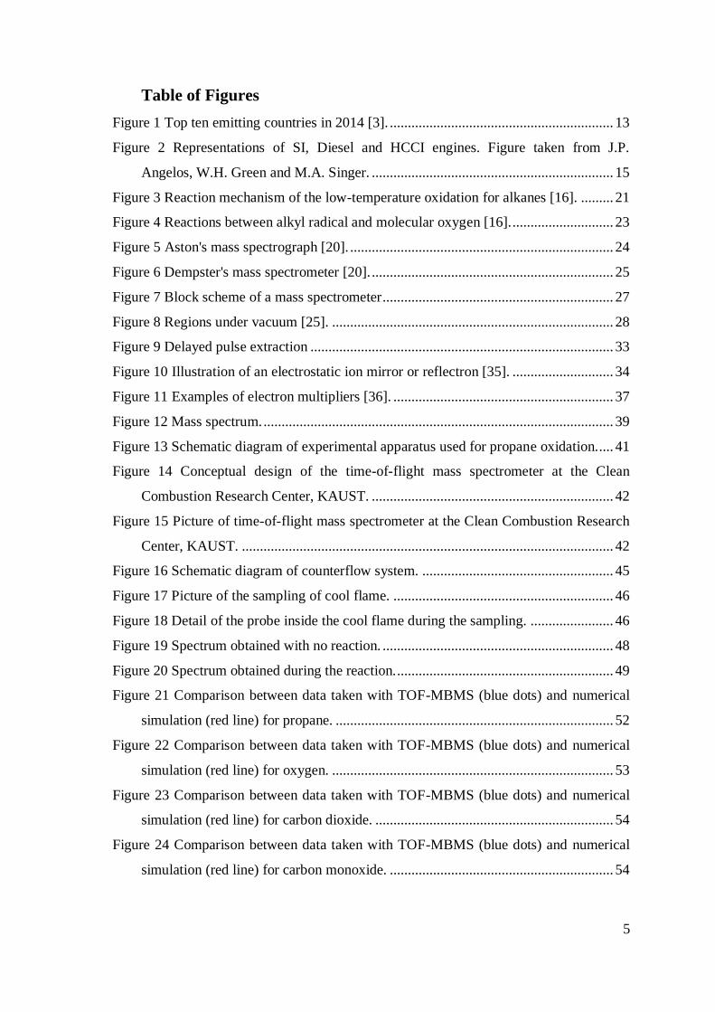
will reach the detector at the same time of the faster one (Figure 9). To improve the
spectral resolution the intensity of the pulse or the time delay can be modified separately.
It is important to note that these two parameters are mass dependent: for species with a
lower m/z ratio, shorter delays or lower voltages are better. As a general rule, for a
known m/z and initial velocity distribution, pulses with high voltage require short time
delays and vice versa. This technique has also the shortcoming that the mass calibration
can be optimised only for a mass range at a time [26].
Figure 9 Delayed pulse extraction
1.2.3.2. Setup of the TOF analyser
For this thesis work we used a MBMS instrument with a reflector time-of-flight as mass
analyser. The reflector TOF provides a more accurate evaluation of the samples.
In a linear TOF, a pulsed laser is focused on a plate where the sample is held. The
voltage to accelerate the ions is applied between the sample holder and a grounded
counter electrode. After the production of the ions, they move towards the detector
following a straight line through the flight tube. The total time-of-flight is slightly
different from the time calculated with eq. (35). To the drift time (td) determined

34
according eq. (35), the time for the process of ionization (t0) and for the acceleration of
the ions (ta) must be added:
𝑡𝑡𝑜𝑡𝑎𝑙 = 𝑡0 + 𝑡𝑎 + 𝑡𝑑
( 40 )
In 1973, Boris Mamyrin, a Russian scientist, has developed a new concept of TOF
analyser [35], called reflector time-of-flight (RTOF) analyser, different from the linear
time-of-flight (LTOF) analyser. The reflector is basically an ion mirror consisting of
several rings at increasing potential. The reflector is situated in front of the ion source
after a field free region: therefore, the ions travel freely to the reflector in which they are
slowed down until they reach zero kinetic energy. After that, the ions are expelled in the
opposite direction, and pass through another field free region towards the detector,
situated on the same side of the ion source (see Figure 10).
Figure 10 Illustration of an electrostatic ion mirror or reflectron [36].
The main job of the reflectron is to correct the kinetic energy gap between two ions with
the same m/z ratio since the one with more energy will go deeper in the ion mirror
spending more time inside it. Thus, the two ions will reach the detector at the same time;

35
moreover, if an ion fragments after the acceleration, the two fragments will have the
same velocity but different kinetic energy because of the different mass. Therefore, in a
RTOF these ions have different flight times according to their mass and will reach the
detector separately. The working principles of RTOF are expressed by the following
formulas: the kinetic energies (Ek) of the parent and the fragment (Ef) ions are,
respectively
𝐸𝑘𝑝 =𝑚𝑝𝑣𝑖𝑥
2
2
( 41 )
and
𝐸𝑘𝑓 =𝑚𝑓𝑣𝑖𝑥
2
2
( 42 )
where mp and mf are the mass of precursor and fragment ion and the velocity (vix) is the
same for both species.
Rearranging equations (41) and (42) we have
𝐸𝑘𝑓 = 𝐸𝑘𝑝
𝑚𝑓
𝑚𝑝
( 43 )
Since the penetration depth is given by 𝑑 =𝐸𝑘
𝑞𝐸 for the precursor and the fragment, we
will obtain respectively
𝑑𝑝 =𝐸𝑘𝑝
𝑞𝐸
( 44 )
and
𝑑𝑓 =𝐸𝑘𝑓
𝑞𝐸=
𝐸𝑘𝑝(𝑚𝑓 𝑚𝑝)⁄
𝑞𝐸
( 45 )

36
So, the penetration depth of the fragment ion can be written as
𝑑𝑓 = 𝑑𝑝
𝑚𝑓
𝑚𝑝
( 46 )
and the flight times for both ions are given by
𝑡𝑟𝑝 =4𝑑𝑝
𝑣𝑖𝑥
( 47 )
and
𝑡𝑟𝑓 =4𝑑𝑓
𝑣𝑖𝑥=
4𝑑𝑝(𝑚𝑓 𝑚𝑝)⁄
𝑣𝑖𝑥= 𝑡𝑟𝑝
𝑚𝑓
𝑚𝑝
( 48 )
The RTOF-MBMS instrument is compatible with pulsed ionization techniques but it
shows the best performances if used in conjunction with the continuous ionization
techniques. This shrewdness can be accomplished changing the setup slightly: the beam
coming from the ion source has to be sent through a small opening to the TOF analyser.
The orthogonal acceleration is the best way to use the continuous ionization with the
TOF: the samples are always ionized and when necessary the application of a voltage
allows deflecting the ion beam inside the flying tube [26].
1.2.3.3. Detector
In the detector the impact of the ions is transformed in an electric current proportional to
their abundance. Several types of detector may be adopted in MS instruments and its
choice depends on the experiment type and the MS setup itself. All the detectors can be
divided in two groups: one class counts the ions with a specific m/z value one at a time
and at the point where they hit the surface; the other detectors count multiple masses at
the same time detecting all the ions hitting the surface [26].

37
1.2.3.4. Electron multiplier (EM) detector
The electron multiplier or secondary electron multiplier (SEM) detector is the most used
and it is the one available on the MBMS instrument used in the internship. It relies on the
photomultiplier tube working concept and it can have different shapes (see Figure 11).
Basically, when an ion hits the first dynode, which produces a secondary electron, an
electron cascade begins and the signal is amplified by a factor of 106. Actually, not
always an electron is emitted, but even positive or negative ions or neutrals can be
emitted: if a negative ion hits the high-voltage (from 3 to 30 kV) dynode, the secondary
particles emitted are positive ions; while if a positive ion strikes the dynode, the
secondary particles released are negative ions and electrons. All the secondary species
are converted in electrons at the first dynode [26, 37].
Figure 11 Examples of electron multipliers [37].
Two kinds of electron multipliers are shown in Figure 10. The one on the left is a
discrete-dynode EM, while on the right the continuous-dynode EM is drawn. The main
difference between them is that the first one is made with singular dynode, while in the
other the inner surface of a curved insulating tube is coated with a resistive film. The
SEM detector is an excellent detector for mass spectrometry because it has high gain (103
– 107), low noise (>1 count /s) and large linear dynamic range (104 – 106) [37].

38
1.2.4. Data Output
The electrical signal acquired must be converted into a compatible format for the output.
For mass analyser like TOF, the system accumulates data for a certain amount of time
and sends them to the data system adding each newly acquired spectrum to the previous
ones. This type of data acquisition is called integrating transient recorder (ITR) or digital
signal averaging (DSA) system. The time-to-digital converter (TDC) is widely used in
TOF mass spectrometer. As already said, when an ion strikes the detector a certain
number of electrons is produced and amplified. If the pulse goes beyond a threshold
value determined by the discriminator, the timing started when the pulse is formed stops.
Thus, each pulse of electrons is timed, and the corresponding value is stored in the
histogram memory as a list and forward to the data system in the form of a spectrum,
with the mass to charge ratio (m/z) as abscissa and the signal intensity as vertical axis.
If more than one ion comes to the detector at the same time, the TDC will count only one
because it is a time counting device. Furthermore, when one ion hits the detector right
after another one, the TDC is not able to count the latter, because there is a dead time
between one registration and another. This limitation affects the measurement accuracy.
Since is possible to acquire for a long time, even small amount of sample can be detected
[26]. The result is a mass spectrum, a so-called “fingerprint” of the species analysed.
Since the abscissa values are related to the molecular weight of the ionized species, the
mass spectrum is easier to interpret than others, such as a gas chromatogram [24].
In Figure 12 is shown, as example, a mass spectrum obtained in a typical oxidation test
of propane. The intensity values in the y-axis have been normalized with respect to the
strongest signal at 40 m/z, which corresponds to the argon. In the following spectrum the
signals at 28, 29, 43 and 44 m/z corresponds to the propane fingerprint, while the ones at
18 and 32 m/z belong to water and oxygen, respectively.

39
Figure 12 Mass spectrum.
1.3. Research objectives
The main objective of this thesis work is to evaluate the performances of the time-of-
flight Molecular Beam Mass Spectrometry (TOF-MBMS) in the analysis of the oxidation
of propane at low temperature. Strong interest has been devoted to the detection of
fleeting species to verify the low-temperature oxidation mechanism proposed by Zádor et
al. [16]. So far, the low temperature oxidation of propane has not been deeply studied
because its less reactivity, due to the short size of the alkyl chain, which limits the chain
branching path [38]. Therefore, the necessary conditions to enhance its reactivity are
close to the explosion limits. Thanks to the characteristics of MBMS where the gaseous
reaction products are transformed into a molecular beam, the reaction is quenched and
also highly reactive species can be detected and analysed. To this aim, we investigated
the oxidation of propane between 750 and 1100 K, with a residence time τ = 1 s and with
molar fractions for C3H8/O2/Ar of 2/13/85 % which corresponds to a Φ equal to 0.77.
Moreover, to verify the quality of the measurements of TOF-MBMS instrument, we
compared the obtained results with those determined with the gas chromatograph (GC).
Then, the experimental results are compared to predicted values to check the adequacy of
the kinetic model used for the simulations. The numerical simulations are performed

40
using the software CHEMKIN PRO with the kinetic mechanism for n-heptane provided
by Politecnico di Milano.
In addition, to explore the versatility of the MBMS apparatus, we studied the detailed
structure of the cool flame activated by ozone in a counterflow setup and determined the
concentration profile of both reactants and products, flowing propane and n-butane as
fuel, separately. To obtain a bi-dimensional flame two burners were disposed facing each
other: the fuel/nitrogen stream flowed from the upper nozzle and it was heated to achieve
the temperature necessary for the ignition of the flame, while, from the lower side,
oxygen and ozone premixed were flowed. The propane tests were performed with a 50%
fuel and 50% nitrogen mixture and an oxygen flow rate of 5 dm3/min which corresponds
to 5.94% of ozone addition. These parameters correspond to a strain rate of 44 s-1. For n-
butane experiments, the mixture was 55/45 % for nitrogen and fuel, respectively; the
flow rate of oxygen was 7 dm3/min with 5.02% of ozone and a strain rate of 61 s-1.
During the experiments, we collected several samples in different points of the bi-
dimensional flame moving the probe from one nozzle to the other. The data obtained
were compared with numerical simulation performed with the kinetic model Aramco
Mech 1.3 both for propane and n-butane.

41
2. METHODOLOGY
2.1 Experimental apparatus specification
2.1.1. Propane oxidation
The experiments were carried out at the Clean Combustion Research Centre (CCRC),
King Abdullah University of Science and Technology (KAUST) using a jet stirred
reactor, well suited for gas phase kinetic studies, within which a mixture of propane,
oxygen and argon were introduced.
Figure 13 represents a schematic illustration of the apparatus used for the oxidation of
propane, while Figure 14 and 15 are a conceptual design and a picture of the instrument,
respectively. The reaction occurs in a jet stirred reactor (JSR) which consists of a 30 cm3
fused silica sphere and it can be modelled as a perfectly stirred reactor [38]. The gas
mixture is introduced into the reactor by means of four jet nozzles differently oriented to
guarantee well-mixed conditions [39]. Two tubes are connected to the reactor, one at the
opposite side of the other; one is for the upstream, where a long, thin fused silica tube is
placed with the lodging for the thermocouple next to it; the tip of this thin tube is placed
right before the reactor. The other tube is for the exhaust gases.
Figure 13 Schematic diagram of experimental apparatus used for propane oxidation.

42
Figure 14 Conceptual design of the time-of-flight mass spectrometer at the Clean Combustion Research
Centre, KAUST.
Figure 15 Picture of time-of-flight mass spectrometer at the Clean Combustion Research Centre, KAUST.

43
The JSR was placed inside an insulated oven equipped with a temperature control. The
temperature inside the reactor was measured with a K-type thermocouple connected to a
temperature reader with an error in the measurement of about ±5 K. The gases were
flowed using four different mass flow controllers provided by MKS. The instrumental
error of the controller of gas flow was estimated to be about 1%. Propane and oxygen
must not be premixed and a mixture of propane (purity 99.5%) and argon (purity
99.999%) is flowed inside the inner tube, while the mixture of oxygen (purity >99.9%)
and argon flows in the bigger tube. We put the 20 cm long, silica fused probe connected
to the MBMS directly inside the downstream tube close to the reactor to sample the
reaction products which are subsequently quenched in a molecular beam.
The experiments were run from 750 to 1100 K at atmospheric pressure, with a residence
time τ = 1 s and molar fractions of C3H8/O2/Ar equal to 2/13/85 %, respectively, which
corresponds to an equivalence ratio of Φ = 0.77. The temperature of the oxidation was
varied from one sampling to the next by 10 K. The residence time of the gas mixture
inside the tube before reaching the reactor is shorter than the residence time inside the
reactor [38]. Since the downstream tube was open, the total flow rate was increased to
1.8 L/min to avoid any intrusion of air inside the reactor.
The instrument used for these experiments was a modified Hiden HPR-60 MBMS
equipped with a Kore time-of-flight mass spectrometer (200 m/z range). The sample was
collected with a quartz 200 mm long probe with a 100 μm orifice. The sampling system
consists in three stages held at different pressure; both the skimmer cones of the first and
second stage are made by nickel; the first stage has a 51 mm long cone with 0.3 mm
orifice and a 34° external angle, the second stage has a 2 mm orifice skimmer cone. The
first stage is held at a pressure of about 10-3 Torr by a turbomolecular pump (Edwards
iXR2206, 2200 dm3/s), while the pressure in the second and third stage is kept at about
10-7-10-8 and 10-8 Torr, respectively, using a turbomolecular pump (Edwards
nEXT240DX) working in both stages at a pumping speed of 240 dm3/s [40]. The TOF-
MBMS has been set to operate with electron energy of 20 eV and an emission of 200 μA
for the ionization of samples; the acquisition time was 180 s for each sampling. In the
experimental procedure, the working temperature was gradually reached by means of the
temperature control of the oven and flowing only the inert gas to uniform the heating
inside the reactor; oxygen and propane were not flowed during the heating to avoid any

44
dangerous situation. Next, both oxygen and propane were flowed while waiting the
temperature was kept stable. In the meantime, we turned on the TOF-MBMS and its
software, necessary to collect the samples; once the experiment was running at the right
temperature we started the sampling. Three samplings were done in each experiment at
constant temperature to check the measurement reproduction.
For the tests performed with the GC (Agilent Technologies 7890A) two detectors were
present in the instrument: a flame ionization detector (FID) and a thermal conductivity
detector (TCD) which analysed the following species: C3H8, O2, CO, CO2, C2H4, C2H2,
C3H6 and CH4.
Since we knew the accuracy of the GC because it was already used in several
experiments, we compared the GC results with the ones from the MBMS to verify the
accuracy of the latter.
2.1.2. Cool flame in counterflow setup
The counterflow setup is a system recently developed by the Clean Combustion Research
Centre (CCRC), KAUST. Its scheme is shown in Figure 16. It consists of two metal
nozzles facing each other, both with inner diameter of 25.4 mm, which allow the
formation of a flat flame; the flows of fuel, oxygen and nitrogen are controlled by three
mass flow controllers provided by MKS. Fuel and nitrogen are mixed and then passes
through two heaters before entering in the upper nozzle. The upper part of the burner is a
311 mm long, alumina ceramic tube with an inner diameter of 32 mm and it is fixed
between two metal bases sealed with high-temperature silicon glue and cement to avoid
any gas leakage. The heating of fuel/nitrogen stream was achieved using a pre-heater and
an external heater (Thermcraft, 1-1/4ID X8L 365W 115V 12”) braided leads, both
electrically controlled using variable transformers to provide constant power. The heating
device and the ceramic tube are surrounded with temperature-resistant insulation to
minimize radiant heat loss. Oxygen and ozone flow from the lower nozzle. An ozone
generator provided by Ozone Solution (TG40) generates ozone starting from pure
oxygen (purity >99.9%) before entering the lower burner. Since the ozone concentration
decreases when the flow of oxygen increases, the oxygen flow is maintained during the
measurements to keep the ozone concentration constant [41, 42]. To measure the ozone

45
concentration in the oxidizer stream we used an ozone monitor (2B Technology Model
106-H) connected to the outlet of the ozone generator. An oxygen flow equal to 5 L/min
was used with propane, so the ozone concentration in the oxidizer flow was 5.94%, while
for butane the flow was 7 L/min and the ozone concentration 5.02%. The two nozzles are
surrounded by a “shield” of nitrogen to separate the flow-field from the surrounding
environment. The distance (L) between the two burners is maintained fixed at 15 mm
which corresponds to a strain rate equal to 44 s-1 in propane experiments, and 61 s-1 for
n-butane flame. The strain rate (a) is defined as the density-weighted gradient of the axial
flow velocity and it is expressed as follow [43]:
𝑎 =2|𝑉2|
𝐿(1 +
|𝑉1|√𝜌1
|𝑉2|√𝜌2
)
( 49 )
Here ρ1 and V1 are the density and the component of the fuel flow velocity normal to the
stagnation plane, respectively, while ρ2 and V2 refer to the oxidizer flow.
Figure 16 Schematic diagram of counterflow system [44].
The experiments were performed at 570 K (±5 K), checked with a K-type thermocouple
placed between the two nozzles close to the upper side. After the temperature reached the
Stagnation Plane
N2 N2 Pre heated fuel
at 570K
N2 N2
O2+O3
Fuel supply
Nitrogen supply
Nitrogen supply
Oxygen supply
MFC
MFC
MFC
MFC
L
O3 generator O3 Monitor

46
chosen value, we removed the thermocouple and inserted the probe of the TOF-MBMS
between the burners. Since we wanted to analyse the structure of the flame (see Figure
17 and 18), we moved the probe from the upper nozzle to the lower side to made eleven
samplings. The first sampling was taken at 1.5 mm from the upper nozzle while the next
ones were done at step of about 1.1 mm proceeding towards the lower side. In this
procedure, a motorized stage (Mitsubishi) mounted under the device moved the whole
system, while the probe height was fixed because connected to the TOF-MBMS.
Figure 17 Picture of the sampling of cool flame.
Figure 18 Detail of the probe inside the cool flame during the sampling.
The experimental heating of the fuel/nitrogen stream required a time of about four hours
until the chosen temperature was reached. For safety reason during the heating only the
inert gas (nitrogen) was flowing. The fuel and the oxygen/ozone streams were opened
only when the temperature to ignite the cool flame was reached, then the TOF-MBMS
was turned on and the sampling started.
2.2. Safety consideration
In any laboratory practice safety is of primary importance. Indeed, all the necessary
safety precautions and equipment were adopted all along the experiments carried out in
47
this thesis work. Since we used flammable and dangerous gases all the instruments were
placed under an isolated and ventilated hood. Thus, all the gaseous species released were
vacuumed to the exhaust system. Since formaldehyde and ozone were used, we used a
respirator with special cartridges for aldehydes and other hydrocarbons, and an ozone
sensor with alarm sound was placed near the working area to detect any leakage.
The oxidation of propane was conducted with 2% of molar fraction for propane and 13%
for oxygen. According to the flammability diagram the lower explosive limit (LEL) is
2.1% for propane in air, while the upper explosive limit (UEL) is 9.5%; since the oxygen
was used at a lower concentration than in air, we were working out of the range of
flammability.
2.3. Data analysis
There are several factors which make the quantitative analysis of chemical species more
complicated with the MBMS than with other instruments. Two of them are the
differences in electron ionization cross-section and mass focusing effects. The mass
focusing effects during the molecular beam formation cause an enrichment of heavier
species since the radial diffusion velocity is higher for lighter species [23]. In addition,
several parameters can be tuned to achieve a more understandable mass spectrum; for
example, the fragmentation of the species can be manipulated varying the electron
energy [24].
The interference problem due to the fact that C3H6, C3H5, C2H4, C2H2 and CH4 are
reaction products in our experiments but can derive also from the fragmentation of
propane and n-butane must be overcome. The assignment of a species signal as product
or as a fragment of propane was guided by the calculation of the ratios of all the signal
areas of propane, from a mass spectrum recorded at low temperature so no reaction
occurred. Then the calculated ratios were subtracted from the corresponding area ratios
of mass spectra resulting from the propane oxidations. In all the tests, we used an
electron energy of 20 eV, that is adequate to ionize all the species and avoids an
excessive fragmentation.

48
Below are shown two spectra collected in propane oxidation experiments. The first
spectrum (Figure 19) was recorded at relatively low temperature (770 K), without any
reaction in progress, as evidenced by the reactant peaks and the absence of any product
signal. At 43 and 44 m/z are visible the peaks of C3H8 and C3H7 while at 28 and 29 m/z
those corresponding to C2H4 and C2H5: this is the fingerprint of propane. The area of the
peaks at 43, 44 and 29 m/z were used to calculate the molar fraction of the propane, while
the one at 28 m/z were used to estimate the ethylene concentration as explained below.
The strongest signal at 40 m/z belongs to the argon, which, being inert, was used to dilute
the mixture fuel/O2 and as internal standard to perform the quantitative analysis. The
weak peak at 18 m/z is due to the residual air humidity.
Figure 19 Spectrum obtained with no reaction.
In the spectrum recorded at higher temperature (910 K), shown in Figure 20, the
intensities of the characteristic peaks of propane (29, 43 and 44 m/z) are lower than
before demonstrating that at this temperature the reaction is running. Indeed, the peaks of
some products clearly appear at 16 m/z, attributed to methane (CH4) and at 15 m/z, to
CH3, which derives from the methane parent ion. In addition, the intensity of the H2O
signal increases. The two peaks almost overlapping each other at 28 m/z are due to
ethylene (C2H4) and carbon monoxide (CO). So, it has been necessary to correctly
attribute each signal to the right species and to measure the areas accordingly before

49
performing the quantitative analysis. A limit of the MBMS technique is that it is not
possible to separate the product mixture into its constituents before the collision with the
accelerated electrons [23]. Other apparent signals are due to: formaldehyde (CH2O),
weak peak at 30 m/z, oxygen at 32 m/z, water cluster, weak peak at 36 m/z according to
Benedikt et al. [45]. At higher m/z there is the fingerprint of propane with the
interference of carbon dioxide (CO2) at 44 m/z. The same procedure adopted for ethylene
was used to overcome this interference.
Figure 20 Spectrum obtained during the reaction.
Once we collected all the spectra, we measured the area of each peak and since we
collected a huge amount of data, we used a software (MATLAB) to process all the
spectra at the same time.
Using the intensity values I taken from the spectra and the sensitivity factor S at a given
temperature, we determined the molar fraction profiles for each species by means of the
following equation
𝑥𝑖 =𝐼𝑖
𝑆𝑖
( 50 )
The sensitivity factor Si includes instrumental parameters and characteristic properties of
analysed species. It is determined by the calibration procedure. Mahnen [46] found out

50
that, if the other parameters remain constant, the sensitivity factor varies with the
temperature in the same manner for all the species. Since the ratio between two species
(Si/Sj) does not change at different temperature the following equation can be used in the
quantitative analysis:
𝑆𝑖
𝑆𝑗=
𝐼𝑖𝑥𝑗
𝐼𝑗𝑥𝑖
( 51 )
In the calibration procedure we determined the ratio of the sensitivity factors of stable
species under analysis with respect to Ar. For the fleeting species C3H5 the sensitivity
factor of the nearest stable species (propane) was used. Since propylene (C3H6) is a stable
species but a cylinder for its calibration was not available, we used, even for this
molecule, the propane sensitivity factor. These data were used to derive the species molar
fractions in the experiments. The ratio of sensitivity factor is measured in the calibration
at room temperature using two gas cylinders with different composition, both with argon
as filler since in all the tests performed we used argon instead of nitrogen as internal
standard to avoid the formation of nitrogen oxides. In the following table the
composition of the cylinders used for the calibration are shown
Cylinder Species %
1
N2 0.0996
O2 0.0997
Ar 0.8007
2
H2 0.05
CH4 0.0488
C2H2 0.0512
CO 0.055
CO2 0.0502
Ar 0.694
Table 3 Cylinder compositions for calibration.
Since the propane was not in the previous gas mixtures, we calibrated it using the same
cylinder (purity 99.5%) used for the experiments and the same flow composition
(C3H8/O2/Ar = 2/13/85 %).

51
Each point for both calibration and experimental measurements is an average of three
samplings. The calculated standard deviation for area measurements is less than 10%.
The uncertainties related to the experimental measurements are not easy to quantify, but
we can estimate an uncertainty of 10-20% for all the species, due to the unstable gas flow
rates.

52
3. RESULTS AND DISCUSSION
3.1 Propane oxidation
In this section, we show the results obtained from the experiments of propane oxidation
in jet stirred reactor, comparing them with the numerical simulation and the data
acquired with the GC. We performed four experiments during which we collected three
acquisitions every 10 K in the range of temperature 750-1100 K. This procedure allowed
us to verify the characteristics of the TOF-MBMS apparatus as analytical device.
The molar fractions obtained for each species have been plotted against the temperature:
in each figure the red line represents the results of the numerical simulation, while the
blue dots are the experimental values of xi derived from the quantitative analysis of the
TOF-MBMS recorded mass spectra. The graph in Figure 21 refers to propane. It shows
that both the results of MBMS and the simulations have very similar trends. The kinetic
model adopted for the simulation underestimates by about 30 K the onset of the reaction:
it is 850 K in the numerical simulation and 880 K in the experimental data. At higher
temperatures a trend reversal is highlighted by a small bump; it is shown in both lines but
at different temperatures: the model predicts the lower reactivity at 1050 K instead of at
990 K, as in the experiments.
Figure 21 Comparison between data taken with TOF-MBMS (blue dots) and numerical simulation (red
line) for propane.

53
The same discrepancy between experiment and simulation for the onset of the reaction is
observed for oxygen whose results are shown in Figure 22. In this chart a slight
difference in the trend of the two data series is apparent, especially at higher
temperatures: the O2 decreasing rate is predicted lower than in the experiments. This
could be due to the characteristics of the kinetic model built to describe the oxidation of
n-heptane. Above 1020 K the experimental data show that the oxygen was almost
finished, while the model predicts a small bump and a residual molar fraction of about
3%. This discrepancy could be due to an inadequacy of model that becomes more
pronounced at high temperature.
Figure 22 Comparison between data taken with TOF-MBMS (blue dots) and numerical simulation (red
line) for oxygen.
The experimental results for carbon dioxide shown in Figure 23 agree well with the
numerical simulation for temperatures below 1030 K. Above that temperature the molar
fraction of CO2 becomes steady at about 3.6%, while the model predicts a stable molar
fraction of 5.7% above 1075 K. The plateau of the experimental data is probably due to
the limited quantity of oxygen at high temperatures. In fact, at 1030 K the oxygen molar
fraction was very low (see Figure 22) affecting the conversion of carbon monoxide into
CO2. Another explanation could be that the kinetic model at these temperatures is not
accurate.

54
Figure 23 Comparison between data taken with TOF-MBMS (blue dots) and numerical simulation (red
line) for carbon dioxide.
In Figure 24 the plotted results for carbon monoxide show that the experiments and the
model follow the same trend up to 1000 K. After this temperature, as for CO2, the molar
fraction for CO calculated from the MBMS data becomes steady at about 2%, while the
model predicts a bell-shape trend, dropping to 0.15% at about 1075 K. These
discrepancies are coherent with those observed for CO2.
Figure 24 Comparison between data taken with TOF-MBMS (blue dots) and numerical simulation (red
line) for carbon monoxide.

55
The comparison between experimental and calculated results for propylene and its allyl
radical are shown in Figure 25 and 26, respectively. In the first chart, the trend of the
MBMS results and the simulation are in good agreement. The maximum value of the
propylene molar fraction from experiment, 0.16%, is about fifty percent of the calculated
one and it is reached at 910 K, a temperature larger than that predicted, 875 K. These
differences could be ascribed to the kinetic model used in the simulation, as confirmed
by the different onset of the reaction in propane chart (see Figure 21).
Figure 25 Comparison between data taken with TOF-MBMS (blue dots) and numerical simulation (red
line) for propylene.
The simulation of the production of the allyl radical (see Figure 26) was done using the
Aramco model because this species is not included in the kinetic model from Polimi. We
were confident to use it because the two models showed the same results for all the other
analysed species. To plot the results two different axes for molar fraction were used
because of the difference between the MBMS data and the numerical simulation that is
about three orders of magnitude. In this case, the differences are very pronounced: the
experimental molar fractions increase with higher rate than those predicted reaching the
maximum value = 0.1% at 910 K. Furthermore, the model predicted a different trend for
this species: the only agreement between the two profiles is the formation of the allyl
radicals at about 850 K. The calculated value at maximum is 0.0002%. A reason for such
a discrepancy could be an overestimation of the allyl radical molar fractions from
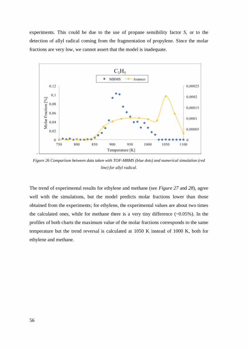
56
experiments. This could be due to the use of propane sensibility factor S, or to the
detection of allyl radical coming from the fragmentation of propylene. Since the molar
fractions are very low, we cannot assert that the model is inadequate.
.
Figure 26 Comparison between data taken with TOF-MBMS (blue dots) and numerical simulation (red
line) for allyl radical.
The trend of experimental results for ethylene and methane (see Figure 27 and 28), agree
well with the simulations, but the model predicts molar fractions lower than those
obtained from the experiments; for ethylene, the experimental values are about two times
the calculated ones, while for methane there is a very tiny difference (~0.05%). In the
profiles of both charts the maximum value of the molar fractions corresponds to the same
temperature but the trend reversal is calculated at 1050 K instead of 1000 K, both for
ethylene and methane.

57
Figure 27 Comparison between data taken with the TOF-MBMS (blue dots) and numerical simulation (red
line) for ethylene.
Figure 28 Comparison between data taken with the TOF-MBMS (blue dots) and numerical simulation (red
line) for methane.
In acetylene chart (see Figure 29) we used two axes for molar fraction because the
difference between experimental values and simulation is about one order of magnitude.
The maximum molar fraction of acetylene is 0.07% at 930 K but in the simulation is
predicted at a temperature about 45 K higher. Even the second experimental maximum at
1025 K is predicted by the model about 50 K higher.

58
Figure 29 Comparison between data taken with the TOF-MBMS (blue dots) and numerical simulation (red
line) for acetylene.
Formaldehyde is the last species analysed with the TOF-MBMS in the experiments of
oxidation of propane at low temperature. The two trends apparent in Figure 30 are
similar: the kinetic model predicts 0.15% as maximum molar fraction at about 890 K,
while the experimental value, 0.35%, is about two times larger and is observed at a
higher temperature, 930 K, like the ones predicted for the other species. Also in case of
formaldehyde a small bump is measured at high temperature: at 1010 K in the
experiments and 1050 K for the simulations.
Figure 30 Comparison between data taken with the TOF-MBMS (blue dots) and numerical simulation (red
line) for formaldehyde.

59
For all the analysed species the temperature difference between the maximum molar
fraction values and those at less reactivity is about 80 K according to the experiment.
Furthermore, in the simulations this difference is larger and change from one species to
another: the maximum gap is 175 K in propylene, while the smallest is 75 K in
formaldehyde.
To verify the data acquired with the TOF-MBMS, we performed the same experiment
analysing the results with the GC, using as detectors both TCD and FID. This test was
run keeping the conditions:
• Temperature: 750-1050 K
• Molar fractions: C3H8/O2/Ar = 2/13/85
• Residence time: τ = 1s
Temperature higher than 1050 K have been avoided in GC experiments for safety reason
to avoid any flame or explosion since both sides of the reactor were closed in this test.
The GC was calibrated by another team, whom assured that the uncertainties of
experimental measurement is lower than 10%. Our results confirm that propane is less
reactive at high temperature than expected according to the side path proposed by Zádor
et al. [16] in the kinetic model. At high temperature, this side path becomes more
relevant and both the alkyl-peroxy radical (ROO⦁) and the hydroperoxy-alkyl radical
(⦁QOOH) leads to the formation of less reactive species such as HO2.
Figure 31 and 32 show the very good agreement between the data from the MBMS and
the GC for propane and oxygen, respectively. In the propane chart, the GC results
confirm the onset of the reaction at 880 K and that propane is less reactive than
predicted. The results for oxygen acquired with MBMS and GC overlap each other up to
990 K while at higher temperature the GC data agree quite well with the predicted ones.
Indeed, at 1050 K the oxygen molar fraction from GC is 3.75%, while that from MBMS
is close to 0.75%. So, to verify the results, we have performed a new test with MBMS at
high temperatures from 940 K to 1100 K. The results confirmed values less than 1% of
the oxygen molar fractions above 1000 K. This behaviour is probably due to the
instability of the reaction at high temperatures or to the formation of a flame inside the
reactor which consumed more oxygen than expected.

60
Figure 31 Comparison between data taken with the TOF-MBMS (blue dots), GC (green line) and
numerical simulation (red line) for propane.
Figure 32 Comparison between data taken with the MBMS (blue dots), GC (green line) and numerical
simulation (red line) for oxygen.
The trends of MBMS and GC results are in good agreement up to 940 K for carbon
monoxide as well, as shown in Figure 33. From 940 K to 1050 K the two data series
significantly differ. The GC results are represented by a bell-shape line while the MBMS
results first increase and then become steady at 2% above 1030 K. The discrepancy of
the two series of experimental data is large but a plausible explanation has not been

61
found. It seems that the propane oxidation process is somewhat affected by uncontrolled
variabiles at high temperatures.
Figure 33 Comparison between data taken with the MBMS (blue dots), GC (green line) and numerical
simulation (red line) for carbon monoxide.
The GC trend for CO2 (see Figure 34) is similar to the MBMS one, but the increase
shown from 930 K to 1050 K is larger in GC results and it is coherent with CO results.
An explanation for CO and CO2 behaviours at high temperatures, could be the suction of
the MBMS. Since the instrument is under vacuum, the suction from the probe is used to
collect the samples and it could disturb the reaction reducing the residence time and not
giving to the CO the necessary time to convert to CO2. On the other hand, this
disturbance can improve the homogeneity of the mixture inside the reactor. However, the
trend showed in CO2 results confirm the behaviour of CO above 1030 K.

62
Figure 34 Comparison between data taken with the MBMS (blue dots), GC (green line) and numerical
simulation (red line) for carbon dioxide.
The GC results for propylene (see Figure 35), show that the maximum molar fraction,
about 0.3%, is close to the value predicted by the kinetic model but it is measured at the
temperature corresponding to the maximum value in MBMS results (910 K).
Furthermore, the GC results do not evidence a decreased reactivity at high temperature
and agree with the simulation.
Figure 35 Comparison between data taken with the MBMS (blue dots), GC (green line) and numerical
simulation (red line) for propylene.
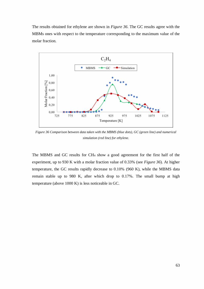
63
The results obtained for ethylene are shown in Figure 36. The GC results agree with the
MBMs ones with respect to the temperature corresponding to the maximum value of the
molar fraction.
Figure 36 Comparison between data taken with the MBMS (blue dots), GC (green line) and numerical
simulation (red line) for ethylene.
The MBMS and GC results for CH4 show a good agreement for the first half of the
experiment, up to 930 K with a molar fraction value of 0.33% (see Figure 36). At higher
temperature, the GC results rapidly decrease to 0.10% (960 K), while the MBMS data
remain stable up to 980 K, after which drop to 0.17%. The small bump at high
temperature (above 1000 K) is less noticeable in GC.

64
Figure 37 Comparison between data taken with the MBMS (blue dots), GC (green line) and numerical
simulation (red line) for methane.
The GC results for acetylene (Figure 38) confirm the trend of MBMS data: the highest
molar fraction at 930 K is lower in the GC line (0.001%) than the one detected with the
MBMS (0.07%).
Figure 38 Comparison between data taken with the MBMS (blue dots), GC (green line) and numerical
simulation (red line) for acetylene.

65
Since both formaldehyde and allyl radicals were not detected by the GC we could not
complete the comparison with the MBMS data. In the overall, the reactant profiles are
confirmed by GC results. Since the uncertainties of the determined molar fractions have
been estimated being in the range 10-20%, the agreement with predicted values for
species such as C3H6, C2H4 and CH4 are satisfactory, while for CO and CO2 the two
series differ at high temperature (above 1030 K). For Acetylene the MBMS and GC
results are inconsistent. The comparison between experiment and simulation for the allyl
radical fleeting species is unsatisfactory, and a overestimation of the experimental values
is suspected.
3.2. Cool flame structure
In this section, the cool flame structure in a counterflow setup is analysed using a TOF-
MBMS instrument, using first propane and then n-butane as fuel. We collected the
samples in several points between the two nozzles to measure the trend of consumption
of the reactants inside this region and to detect which products are mainly formed. To
compare the experimental data with model predictions numerical simulations were
performed with n-heptane model provided by Polimi for propane, and Aramco Mech 1.3
for butane. To favour the understanding of these results, we show again the schematic
diagram of the cool flame in Figure 39.

66
Figure 39 Schematic diagram of cool flame system [44].
3.2.1. Propane flame
The experimental measurements and the numerical simulation of the structure of the
propane cool flame are represented in Figures 40 and 41, respectively. The trends of the
intensities of the mass spectra signals for the reactants (C3H8, N2, O2 and O3), between
the two nozzles, are shown. The position of the propane cool flame is obtained from
inspection of Figure 40 at the crossing between oxidizer and fuel streams. It results that
it is closer to the oxidizer side and not in middle of the two duct nozzles, as predicted by
the model. The difference of the predicted and experimental flame locations is about 0.15
cm and could be caused by the sampling probe [47], or due to the inefficiency of the
model to predict the right position of the flame. The shape of the experimental profiles of
the oxidizer and fuel streams evidences that the reaction rate is low at low temperature:
the fuel diffuses into the oxidizer and vice versa for several millimetres after the crossing
point both in experiment and simulation.
Stagnation Plane
N2 N2 Pre heated fuel
at 570K
N2 N2
O2+O3
Fuel supply
Nitrogen supply
Nitrogen supply
Oxygen supply
MFC
MFC
MFC
MFC
L
O3 generator O3 Monitor
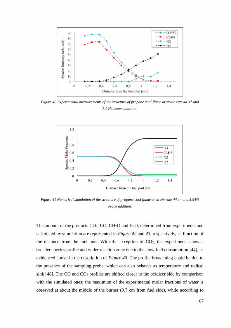
67
Figure 40 Experimental measurements of the structure of propane cool flame at strain rate 44 s-1 and
5.94% ozone addition.
Figure 41 Numerical simulation of the structure of propane cool flame at strain rate 44 s-1 and 5.94%
ozone addition.
The amount of the products CO2, CO, CH2O and H2O, determined from experiments and
calculated by simulation are represented in Figure 42 and 43, respectively, as function of
the distance from the fuel port. With the exception of CO2, the experiments show a
broader species profile and wider reaction zone due to the slow fuel consumption [44], as
evidenced above in the description of Figure 40. The profile broadening could be due to
the presence of the sampling probe, which can also behaves as temperature and radical
sink [48]. The CO and CO2 profiles are shifted closer to the oxidizer side by comparison
with the simulated ones; the maximum of the experimental molar fractions of water is
observed at about the middle of the burner (0.7 cm from fuel side), while according to

68
the simulation it should be aligned with the other peaks at about 0.8 cm from the fuel
port.
Figure 42 Experimental measurements of the structure of propane cool flame at strain rate 44 s-1 and
5.94% ozone addition.
Figure 43 Numerical simulation of the structure of propane cool flame at strain rate 44 s-1 and 5.94%
ozone addition.
3.2.2. N-butane flame
Experimental measurements and numerical simulations for C4H10, N2, O2 and O3 are
shown in Figure 44 and 45, respectively. As for propane, the position of the cool flame is
close to the oxidizer side, while in the simulation it is near to the stagnation point situated

69
in the middle of the burner. The difference between the experimental and calculated
flame positions for n-butane is two times (~0.3 cm) that for propane flame. The position
does not change if the sampling probe is removed. As observed in case of propane, the
two streams diffuse one into the other confirming the low reaction rate at low
temperature.
Figure 44 Experimental measurements of the structure of n-butane cool flame at strain rate 61 s-1 and
5.02% ozone addition.
Figure 45 Numerical simulation of the structure of n-butane cool flame at strain rate 61 s-1 and 5.02%
ozone addition.
The results for CO, CO2, H2O and CH3CHO produced by n-butane cool flame are shown
in Figure 46 and 47. The species profiles are broader than predicted by the kinetic model
and the maxima for three of them are observed at the flame position, i.e. at about 0.95 cm

70
from fuel port. The CH2O shows two maximum values very close to the oxidizer nozzle
differently from simulation.
Figure 46 Experimental measurements of the structure of n-butane cool flame at strain rate 61 s-1 and
5.02% ozone addition.
Figure 47 Numerical simulation of the structure of n-butane cool flame at strain rate 61 s-1 and 5.02%
ozone addition.
In Figures 48 and 49 are illustrated the model predictions of the temperature profile and
molar fractions of some species, in the propane and n-butane flame, respectively. In both
cases the products molar fractions indicate the location of the reaction zone at about 0.8
cm from the fuel nozzle, in agreement with the temperature maximum.

71
Figure 48 Numerical simulation structure of propane cool flame with temperature profile at strain rate 44
s-1 and 5.94% ozone addition.
In Figure 49 also the molar fraction of the ketohydroperoxide NC4KET13, fleet species
included in the kinetic mechanism, is shown. Its shape indicates that NC4KET13 is
formed and consumed to produce most of the CH2O. Inside the flame, since the
temperature is slightly higher, the QOOH beta scission occurs and leads to the formation
of CH2O and OH. Going away from the flame the temperature decreases and the
remaining fuel, which diffuses through the stagnation plane, reacts to form QOOH and
O2QOOH which consequently reacts to produce ketohydroperoxide [44].
Figure 49 Numerical simulation structure of n-butane cool flame with temperature profile at strain rate 61
s-1 and 5.02% ozone addition.

72
4. CONCLUSION
The aim of this project was to use the time-of-flight mass spectrometer (TOF-MBMS) to
study the low-temperature oxidation of propane in jet stirred reactor and the structure of
the propane and n-butane cool flames in counterflow setup. The results obtained are
compared with numerical simulation performed using the software CHEMKIN Pro with
n-heptane model (Polimi) and Aramco Mech 1.3. To verify the characteristics of the
MBMS technique as analytical tool we repeated the propane oxidation tests, in the same
conditions, analysing the exhaust gases with the GC. The experimental results obtained
from MBMS and GC instrumentations are in good agreement confirming the fine
performances of the TOF-MBMS. Only for acetylene the molar fraction detected by the
GC is one order of magnitude lower than that from the mass spectrometer. The
comparison with the simulations shows that the onset of propane oxidation is predicted
by the model at 30 K lower than in the experiments. The molar fraction profiles for all
the analysed stable species (C3H8, O2, CO, CO2, C3H6, C2H4, C2H2, CH4 and CH2O)
measured by MBMS are similar to the predicted ones with some exceptions, as far as the
temperature and maximum molar fraction values are concerned. At high temperature,
above 1000 K, the O2 molar fraction is low (~0.8%) during the experiment, while CO
and CO2 become steady at 2% and 3.6%, respectively, probably due to the lack of
oxygen. On the other hand, at 1100 K the model predicts molar fractions of 3%, 0.2%
and 5.7% for O2, CO and CO2. This discrepancy could derive from some uncorrected
kinetic constants of the reactions adopted in the model. Furthermore, the oxidation
decreases its reactivity at about 990 K, as shown by the small increasing in molar
fraction for propane and all the hydrocarbons produced. This behaviour is confirmed by
simulation but at higher temperature, 1050 K. A smaller propensity in reactivity could be
due to the negative temperature coefficient (NTC), typical for most of the hydrocarbons.
The application of TOF-MBMS as analytical device in the cool flame experiments with
the counterflow setup was satisfactory. It allowed the determination of the trend of the
reactants (propane and n-butane) and some products such as H2O, CO, CO2, CH2O and
CH3CHO, as function of the distance from the fuel port. The comparison of experimental
results with the numerical simulations was encouraging. It resulted that the flame
position is situated on the oxidizer side at 0.8 cm and 0.9 cm, for propane and n-butane,

73
respectively. Indeed, the propane cool flame is closer to the stagnation plane than the
butane one, as confirmed by the direct visualization of the flame during the experiment.
Furthermore, it resulted that the consumption rate of the fuels at low temperature is lower
than predicted. The largest values of the product molar fractions are detected near the
oxidizer nozzle both in propane and n-butane experiments. The only exception is water,
in propane flame, which is closer to the middle of the burners than in the n-butane one.
The difference in position between the streams crossing and the reaction zone is well
predicted by the model. However, the experimental reaction rate is lower than expected,
as evidenced by the profile broadening in the product species. It seems that some aspects
of the adopted kinetic models should be revised.
Some possible future projects could be the study with the TOF-MBMS of other fuels in
different setup. The detection of radical species is possible but a reliable quantitative
analysis of labile species can be afforded through a careful setting of the instrument
parameters, such as electron energy and acquisition time.
74
5. BIBLIOGRAPHY
[1] K. K. Kuo, Principles of Combustion, John Wiley & Sons, INC..
[2] EU Commission, DG ENER, Unit A4, “Energy datasheet: EU-28 countries,” 2017.
[3] IEA, “Key CO2 Emission Trends,” IEA - Int. Energy Agency, 2016.
[4] N. Hansen, T. A. Cool, P. R. Westmoreland and K. Kohse-Hoingaus, “Recent
contributions of flames-sampling molecular-beam mass spectrometry to a
fundamental understanding of combustion chemistry,” Progress in Energy and
Combustion Science, no. 35, pp. 168-191, 2009.
[5] J. B. Heywood, Internal Combustion Engine Fundamentals, 1988.
[6] U.S. Department of Energy, “Just the basics: Diesel Engine,” 2003.
[7] C. K. Westbrook, “Chemical Kinetics of Hydrocarbon Ignition in Practical
Combustion Systems,” in Proceedings of the Combustion Institute, 2000.
[8] S. Saxena and I. D. Bedoya, “Fundamental phenomena affecting low temperature
combustion and HCCI engines, high load limits and strategies for extending these
limits,” Progress in Energy and Combustion Science, pp. 1-32, 2013.
[9] R. Fernandes, “Combustion Chemistry,” in Handbook of Combustion, vol. 1, Wiley-
VCH, 2010, pp. 27-52.
[10] M. Janbozorgi, K. E. Far and H. Metghalchi, “Combustion Fundamentals,” in
Handbook of Combustion, Wiley, 2010.
[11] A. F. Sarofim and K. E. Kelly, “Fundamentals and Safety,” in Handbook of
Combustion, vol. 1, Wiley-VCH, 2010.
[12] S. R. Turns, An Introduction to Combustion, Mc-Graw-Hill Higher Education,
2000.
[13] F. Battin-Leclerc, “What do we really know about the low-temperature oxidation of
alkanes?,” in European Combustion Meeting, 2015.
[14] R. W. Walker and C. Morley, “Low-temperature combustion and autoignition,” in
Basic chemistry of combustion, Elsevier, 1997, pp. 1-124.
[15] S. H. Robertson, P. W. Seakins and M. J. Pilling, “Elementary reactions,” in Basic
chemistry of combustion, Elsevier, 1997, pp. 125-234.

75
[16] J. Zádor, C. A. Taatjes and R. X. Fernandes, “Kinetics of elementary reactions in
low-temperature autoignition chemistry,” Progress in Energy and Combustion
Science, no. 37, pp. 371-421, 2011.
[17] E. Ranzi, C. Cavallotti, A. Cuoci, A. Frassoldati, M. Pelucchi and T. Faravelli,
“New reaction classes in the kinetic modelling of low temperature oxidation of n-
alkanes.,” Combustion and Flame, no. 162, pp. 1679-1691, 2015.
[18] J. H. Gross, Mass Spectrometry, Springer, 2004.
[19] H. Kienitz, “Einfuhrung,” Massenspektrometrie, 1968.
[20] A. Maccoll, “Mass Spectrometry, Historical Perspective,” in Encyclopedia of
Spectroscopy and Spectrometry, Elsevier, 2010, pp. 1452-1458.
[21] American Society for Mass Spectrometry (ASMS), “What is Mass Spectrometry”.
[22] E. de Hoffmann and V. Stroobant, Mass Spectrometry: Principle and Applications,
John Wiley and Sons, Ltd, 2007.
[23] D. L. Carpenter, S. P. Deutch and R. J. French, “Quantitative Measurement of
Biomass Gassifier Tars Using a Molecular-Beam Mass Spectrometer: Comparison
with Traditional Impinger Sampling,” Energy & Fuels, no. 21, pp. 3036-3043, 2007.
[24] R. J. Evans and T. A. Milne, “Molecular Characterization of the Pyrolysis of
Biomass,” Energy & Fuels: an american chemical society journal, vol. 1, no. 2, pp.
123-137, 1987.
[25] H. Analytical, High Pressure HPR60 Sampling System Manual, Warrington.
[26] E. de Hoffmann and V. Stroobant, Mass Spectrometry: Principles and Applications,
Wiley, 2007.
[27] T. a. J. R. Bentley, “Mechanism and structure in mass spectrometry: a comparison
with other chemical processes,” Advances in Physical Organic Chemistry, vol. 8,
1970.
[28] J. T. Watson, “Electron Ionization Mass Spectrometry,” in Encyclopedia of
analytical chemistry: applications, theory and instrumentation, vol. 13, Wiley,
2000, pp. 11680-11694.
[29] T. D. M. C. Lifshitz, “Mass Spectrometry, Ionization Theory,” in Encyclopedia of
Spectroscopy and Spectrometry, Elsevier, 2010, pp. 1459-1469.
[30] S. Meyerson and R. Van der Haar, “Multiply Charge Organic Ions in Mass Spectra,”

76
J. Chem. Phys., no. 37, pp. 2458-2462, 1962.
[31] NIST (National Institute of Standard and Technology), 2015. [Online]. Available:
www.nist.gov.
[32] W. E. Stephens and M. M. Wolff, “A pulsed mass spectrometer with time
dispersion,” Phys. Rev., no. 69, p. 691, 1946.
[33] A. E. Cameron and D. F. Eggers, Jr., “An ion "velocitron",” Oak Ridge, 1948.
[34] S. R. Weinberger, S. Davis, A. Makarov, S. Thompson and R. Purves, “Time-of-
flight Mass Spectrometry,” in Encyclopedia of Analytical Chemistry, Wiley, pp.
11915-11971.
[35] B. A. Mamyrin, V. I. Karctaev, D. V. Shmink and V. A. Zagulin, “The Mass
Reflectron, a New Nonmagnetic Time-of-flight Mass Spectrometer with High
Resolution,” Sov. Phys. JETP, no. 37, pp. 45-48, 1973.
[36] K. G. Standing and W. Ens, “Time of Flight Mass Spectrometers,” in Encyclopedia
of Spectroscopy and Spectrometry, Elsevier, 1999, pp. 2360-2365.
[37] D. W. Koppenaal, C. J. Barinaga and M. B. Denton, “Mass Spectrometry
Detectors,” Anal. Chem., pp. 429A-427A, 2005.
[38] M. Cord, B. Husson, J. C. L. Huerta and O. Herbinet, “Study of the low temperature
oxidation of propane,” The journal of physical chemistry, no. 116, pp. 12214-12228,
2012.
[39] M. de Joannon, A. Cavaliere, T. Faravelli, E. Ranzi, P. Sabia and A. Tregrossi,
“Analysis of process parameters for steady operations in methane mild combustion
technology,” in Combustion Institute, 2005.
[40] A. B. S. Alquaity, J. Han, M. Chahine, H. Selim, M. Belhi, M. S. Sarathy, F. Bisetti
and A. Farooq, “Measurements of positively charged ions in premixed methane-
oxygen atmospheric flames,” Combustion science and technology, 2016.
[41] A. A. Al Omier, “Ozone Activated Cool Diffusion Flames of Butane Isomers in a
Counterflow Facility,” 2017.
[42] S. H. Won, B. Jiang, P. Diévart, C. H. Sohn and Y. Ju, “Self-sustaining n-heptane
coll diffusion flames activated by ozone,” in Combustion Institute, 2015.
[43] S. Humer, R. Seiser and K. Seshadri, “Non-premixed and premixed extinction and
autoignition of C2H4, C2H6, C3H6 and C3H8,” in Proceeding of Combustion

77
Institute 29, 2002.
[44] A. Alfazazi, A. Al-Omier, A. Secco, H. Selim, Y. Ju and S. M. Sarathy, “Cool
diffusion flames of butane isomers activated by ozone in the counterflow (Submitted
to the journal waiting for publishing),” Combustion and flames, 2017.
[45] J. Benedikt, D. Ellerweg, S. Schneider, K. Rügner, R. Reuter, H. Kersten and T.
Benter, “Mass spectrometry of positive ions and neutral species in the effluent of an
atmospheric pressure plasma with hexamethyldisiloxane and oxygen,” Journal of
Physics D: Applied Physics, no. 46, 2013.
[46] G. Mahnen, Université catholique de Louvain, Belgium, 1973.
[47] J. K. Lefkowitz, S. H. Won, Y. Fenard and Y. Ju, “Uncertainty assessment of
species measurements in acetone counterflow diffusion flames,” Proceedings of the
Combustion Institute, no. 34, pp. 813-820, 2013.
[48] U. Struckmeier, P. Oßwald, T. Kasper, L. Böhling, M. Heusing, M. Köhler, A.
Brockhinke and K. Kohse-Höinghaus, “Sampling Probe Influences on Temperature
and Species Concentrations in Molecular Beam Mass Spectroscopic Investigations
of Flat Premixed Low-pressure Flames,” Z. Phys. Chem., no. 223, pp. 503-537,
2009.
[49] N. Leplat, P. Dagaut, C. Togbé and J. Vandooren, “Numerical and experimental
study of ethanol combustion and oxidation in laminar premixed flames and in jet-
stirred reactor,” Combustion and Flames, no. 158, pp. 705-725, 2011.
Top Related