Corporate Swap Use and Its Effect on Swap Spreads

Christopher Paul Lin

Professor Edward Tower, Faculty Advisor

Honors Thesis submitted in partial fulfillment of the requirements for Graduation with Distinction in Economics in Trinity College of Duke University

Duke University

Durham, North Carolina April 2007

Acknowledgements

Many thanks to everyone who helped me put this together. Professor Tower deserves special recognition for his guidance and I am extremely grateful for the advice and comments provided by Professor Hagy and the students in Economics 198/199S.

2

Abstract

Interest rate swaps are financial derivatives that allow people to speculate on interest rates or hedge certain interest rate exposures. Corporations, in particular, can use the swap market to effectively change fixed rate debt into floating rate debt or vice versa. This paper empirically tests whether debt issuance by financial firms has a measurable effect on the relative pricing of swaps in the market. I hypothesize that upon issuing debt, these corporations enter into pay-floating, receive-fixed swaps which, ceteris paribus, would decrease the swap spread. I find that in some cases debt issuance does have a statistically significant tightening effect.

3

I. Introduction

The interest rate swap market is one of the largest and most liquid derivative

markets today. Estimates place the notional amount outstanding in interest-rate and

currency swap contracts at more than $170 trillion in 2006, up from $3 trillion in 1991

(BIS, 2006). The size of the swap market, therefore, dwarfs the amount outstanding of

U.S. Treasury bonds, which was only $5.7 trillion in June 2001 (Liu, 2002). The growth

of the interest rate swap market has made it an increasingly popular choice for a variety

of market participants to trade interest rates.

Interest rate swaps are best conceptualized as a simple exchange of cash flows

between two counterparties for a given time period. In the most basic fixed-for-floating

swap counterparty A pays a floating interest rate (usually 3 month LIBOR1) on a

predetermined notional amount and in return receives a fixed interest rate on the same

notional amount from counterparty B. This exchange of cash flows occurs periodically,

typically every six months or one year, for the duration of the swap. The fixed rate which

counterparty A receives is the swap rate quoted in the market. At any given time, the

quoted swap rate is the fixed rate which gives the swap a present value of zero when the

swap begins.

Swap rates are published every day by financial publications such as the Wall

Street Journal and some online services provide constantly updated swap rates throughout

the day, even though they are not traded on any central exchange. If interest rates

decrease (increase), the value of the swap to the counterparty which receives fixed

becomes positive (negative). This behavior makes receiving fixed in swaps analogous to

1 LIBOR stands for the London Interbank Offered Rate. Published daily by the British Bankers Association, it represents the interest rate at which banks lend money to one another in the London interbank market. It is widely used as a short term benchmark interest rate.

4

owning traditional interest rate securities. Paying fixed in swaps, therefore, is analogous

to selling an interest rate security. 2

Multiple authors have investigated corporations’ motivations for using swaps.

One reason corporations may use the swap market is to better match their assets and

liabilities. Consider a bank who wishes to issue long term debt. The bank’s income is

generated by loans and it has liabilities in the form of short term deposits. Therefore both

its income and its primary liabilities are tied to floating rates so ideally the bank would

want to issue floating rate debt. However, since market demand for long term floating

rate debt is extremely limited, the bank must issue fixed rate debt. In order to simplify its

liability management, the bank may enter into a swap in which they pay floating and

receive fixed. Even though they have issued fixed rate debt, they are essentially able to

transform all of their liabilities into floating rate liabilities. There are currently no studies

which empirically test this hypothesis. Another reason corporations may use the swap

market is to take advantage of information asymmetries (Titman, 1992). A corporation

with favorable nonpublic information about its future may choose to borrow short term

(at floating rates), because as the information becomes public, the company will

presumably face lower borrowing costs. However, this exposes the company to interest

rate risk; if interest rates rise, the borrowing costs also rise, even if the prospects of the

business are entirely unrelated to the level of interest rates. To solve this problem, the

corporation can enter into an interest rate swap to pay fixed and receive floating.

Since swaps have become such actively traded interest rate derivatives,

investigating how they behave relative to the other primary interest rate instrument, U.S.

Treasury debt securities, seems reasonable. This behavior is quantified in the swap 2 For further details and diagrams about the mechanics of swaps, refer to Section III of this paper

5

spread, which is the difference between the quoted fixed rate on a traditional fixed-for-

floating or “vanilla” swap and the yield on the Treasury security with an equivalent

maturity. The rate on the swap is almost always higher and these spreads typically range

between 20 and 100 basis points. Understanding the dynamics of the swap spread should

be a priority for anyone who uses swaps because changes in the spread cause swaps to

behave differently compared to traditional government debt. To gain intuition for how the

swap spread behaves, suppose the government unexpectedly announces a large amount of

new debt they will be bringing to the market. Although this does not change the

fundamental outlook on the path of interest rates in the United States, yields on Treasury

notes will increase in order to digest the new supply, and the swap spread will narrow as

a result. If people could have predicted this move in advance they would have preferred

to receive fixed in a swap relative to holding the Treasury debt. Alternatively, they could

short sell Treasuries and receive fixed in swaps to limit their direct exposure to interest

rates and hope to profit from a decrease in the swap spread.

Some of the literature has attempted to identify all of the factors which influence

the swap spread including the spread between LIBOR and the general collateral (GC)

repo rate on Treasuries, government bond issuance, the slope and level of the yield curve,

and risk and liquidity premiums (Cortes, 2003)3. But despite the strand of literature

which focuses on the motivations of corporations to use swaps in conjunction with debt

issuance, no models of swap spreads explicitly include corporate debt issuance as a

determining factor.

In this paper I quantitatively examine the effect of corporate debt issuance, in

particular that of highly rated financial firms, on the swap spread and how the 3 Further explanation of these factors can be found in Section III

6

relationship has changed over time as the swap market has expanded. The financial press

has recognized the existence of this relationship: Barrett and Marine (2006) identify five

different financial corporations issuing debt with a total value of over $10 billion during a

particularly active week in the investment grade credit market and note that this issuance

would probably put pressure on swap spreads to tighten, reasoning that the issuers would

enter swaps in which they pay floating and receive fixed. This paper aims to take an

academic perspective by using a regression framework to analyze whether issuance of

debt by financial corporations empirically causes swap spreads to narrow. In addition, I

will investigate if any other conclusions can be made regarding the timing of the

tightening or the type of firm whose issuance has the greatest effect. Given my data set, I

find that swap spreads do generally decrease upon financial debt issuance, though this

result is not always statistically significant. As the swap market has grown, this effect has

actually become less significant. The spread narrowing exists both on days that the debt

is issued and on days when future issuance is announced, and is statistically significant

for investment brokerage firms.

The paper will continue as follows: Section II provides a more detailed overview

of the relevant literature regarding motivations for corporations to use swaps and the

determinants of swap spreads. Section III places the empirical analysis of this paper

within a theoretical framework of how swap spreads should behave. Section IV discusses

the data used in the tests, which are described and performed in Section V. Section VI

concludes the paper with a summary of the results and commentary on the implications of

the study.

7

II. Literature Review

Since swaps are a relatively recent financial innovation, the body of literature

covering them is small, yet growing. As mentioned in the introduction, there is a

collection of papers which aim to explain corporate decisions regarding financing

decisions and the use of swaps, and a handful which address determinants of the swap

spread, yet none which explicitly connect the two ideas together as this paper aims to do.

The literature also emphasizes the decision for non-financial firms to enter into pay-fixed

swaps, spending little time focusing on why firms may wish to receive fixed in swaps. By

empirically estimating whether the quantity of debt issued by financial firms has an

observable effect on the swap spread, I hope to potentially identify an area for further

theoretical research in the swap literature.

There are two prevalent theories regarding why firms may pay fixed in standard

fixed-for-floating swaps; Bicksler and Chen (1986) enumerate the first theory that market

imperfections may cause certain corporations to have a comparative advantage borrowing

fixed and others to have an advantage borrowing floating4. If a firm with an advantage

borrowing floating wishes to borrow at a fixed rate and the opposite holds true for

another firm, both parties receive economic benefits by entering into a swap with each

other. In particular, low credit-quality firms must borrow at a higher rate than high credit-

quality firms in both the short term floating rate market and the long term fixed rate

market. The spread between borrowing costs, however, is wider for longer maturity fixed

rate debt than short term floating rate debt. Therefore if the lower credit-quality firm

wants to borrow at a fixed rate it benefits by borrowing short term at a floating rate and

4 Borrowing fixed refers to a debt contract in which the corporation must make the same interest payment on the loan, regardless of what happens to interest rates. Borrowing floating refers to a loan whose interest payments vary, typically as a spread over a short term interest rate such as LIBOR.

8

paying fixed in a swap. As a result, this theory predicts that low credit-quality firms tend

to pay fixed and receive floating, while implying, though never explicitly stating, that

firms with better credit benefit when they receive fixed and pay floating.

A disadvantage of this theory is that it neglects the credit risk that the higher

credit-quality firm assumes when entering into the swap. Theoretically, the party

receiving fixed from the lower credit-quality firm should require additional compensation

for the additional risk that the lower credit-quality firm cannot make its payments. In

practice, however, this consideration is quite small and pricing of swaps generally does

not depend on the credit quality of the counterparty. One reason is that the actual dollar

exposure of a given counterparty is quite small relative to the total notional value of the

swap, especially once payments are netted. Litzenberger (1992) hypothesizes that swaps

are not sensitive to credit rating differences because the treatment of swaps in the event

of bankruptcy is asymmetric (it favors the solvent party), swaps sometimes contain

“credit triggers” which allow for early cash settlement in the event of a credit downgrade,

and firms with weak credit are often required to collateralize the swaps. Along the same

lines, Duffie and Huang (1996) estimate that if the credit spread between two

counterparties involved in a swap is 100 basis points, then the relevant adjustment to the

swap rate should be less than 1 basis point. In other words, the effect of the credit quality

differential on the swap rate is extremely small.

The second primary theory for pay-fixed use of interest rate swaps involves

information asymmetries. Titman (1992) builds on previous theories that borrowers with

favorable non-public information about their prospects prefer to enter into a series of

short term floating rate loans with the idea that their interest rates on these loans will

9

decrease as the information becomes public. These short term loans, however, expose

them to interest rate risk. In an environment of interest rate uncertainty, Titman proposes

that they can enter into a long term swap contract to pay fixed and receive floating.

Unfortunately Titman cannot extend this theory to rationalize why some firms enter into

swaps to pay floating. He resolves this issue by reasoning that because there is an excess

demand to pay fixed, swaps are priced to favor those who receive fixed. This argument

seems tenuous, especially if I can show that corporate debt issuance by large financial

firms moves the swap market in a direction that makes paying fixed relatively more

attractive.

Both of these theories have been subjected to numerous empirical tests to verify

their validity, and the results are encouraging. Simkins and Rogers (2006) find strong

evidence supporting Titman’s theory, noting that firms which synthetically finance at a

fixed rate by borrowing floating and swapping into fixed are more likely than other firms

to have their credit quality upgraded. Li and Mao (2003) extend Titman’s theory to

include firms using long term floating rate bank loans, rather than a sequence of short

term floating rate loans. In their thorough empirical analysis, they find results that

support both the Bicksler and Chen theory and the Titman theory. They discover that

firms who receive fixed generally have superior credit ratings compared to those who pay

fixed. They also find evidence for their theory that fixed rate payers have a higher

proportion of bank loans than floating rate payers. Another intriguing result with

implications for this paper is that in general, fixed payers are smaller than floating payers.

As a result, one might expect a significant impact on the swap spread when floating

payers (i.e. large financial firms) enter into swap contracts.

10

Only Gnanakumar Visvanathan (1998) directly addresses the question of who

exactly pays floating in swaps. In addition to the simple conjecture that high credit

quality firms pay floating in swaps to share benefits with lower quality firms who pay

fixed, Visvanathan hypothesizes that a duration mismatch between assets and liabilities

could provide an incentive for a firm to enter into a receive fixed swap. Suppose the

interest rate sensitivity of the liabilities of a firm is higher than that of the assets so that

when interest rates decrease, the value of the firm’s liabilities increase by more than its

assets. To resolve this problem, the firm can pay floating and receive fixed to increase the

duration of its assets. Empirically Visvanathan finds no evidence to support either of

these explanations for why firms pay floating. He notes, however, that the variable he

uses to test the asset-liability duration mismatch actually tests the relative length of asset

and liability maturities. Additionally he performed this study based on data from 1992

and 1993 when the swap market was still relatively young. This paper utilizes more

recent data in searching for empirical evidence that financial firms noticeably influence

the swap market when paying floating.

The effect, if observed, will occur on the swap spread. Much of the more recent

literature regarding swaps has focused on the behavior of the swap spread, though there

are still fewer papers than those discussing the corporate financing choice and they are

typically more focused on gathering empirical evidence than developing theory. Fehle

(2003) develops a model in which swap spreads are driven by expected LIBOR spreads5

and market structure, in addition to default risk. Expectations of increases in the LIBOR

5 The LIBOR spread is the difference between the rate on LIBOR and the rate on a given government security of the same maturity. They are typically positive because LIBOR is subject to default in the case of a banking system failure, whereas it is implicitly assumed that government securities are essentially risk-free.

11

spread would cause a pay floating user of a swap to demand additional compensation in

the form of a higher spread to Treasuries. His theory on market structure recognizes the

deficiency in the literature in explaining the types of floating payers and hypothesizes

that these players enter the market only because of the advantages they can share with the

fixed rate payers. He finds that these two additional factors do have an effect on swap

spreads. Liu, Longstaff, and Mandel (2002) find that the liquidity differential between

U.S. Treasury debt securities has a tangible effect on swap spreads. This is because on-

the-run Treasuries are considered extremely liquid instruments and therefore have a

liquidity premium built into the price6. If overall liquidity decreases, this premium will

rise, driving prices of these Treasuries up and resulting in a wider swap spread. Finally,

Cortes (2003) empirically identifies and analyzes a number of factors which may affect

the swap spread. These include expectations of government bond issuance, the slope of

the yield curve, risk and liquidity premiums, and mortgage prepayment hedging.

6 In other words, investors give the most actively traded Treasury securities added value because they are easily bought and sold in the secondary market.

12

III. Theoretical Framework

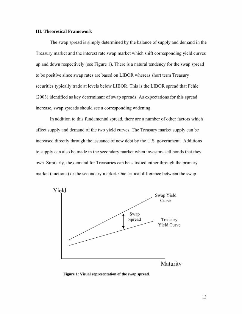
The swap spread is simply determined by the balance of supply and demand in the

Treasury market and the interest rate swap market which shift corresponding yield curves

up and down respectively (see Figure 1). There is a natural tendency for the swap spread

to be positive since swap rates are based on LIBOR whereas short term Treasury

securities typically trade at levels below LIBOR. This is the LIBOR spread that Fehle

(2003) identified as key determinant of swap spreads. As expectations for this spread

increase, swap spreads should see a corresponding widening.

In addition to this fundamental spread, there are a number of other factors which

affect supply and demand of the two yield curves. The Treasury market supply can be

increased directly through the issuance of new debt by the U.S. government. Additions

to supply can also be made in the secondary market when investors sell bonds that they

own. Similarly, the demand for Treasuries can be satisfied either through the primary

market (auctions) or the secondary market. One critical difference between the swap

Maturity

Yield

Treasury Yield Curve

Swap Yield Curve

Swap Spread

Figure 1: Visual representation of the swap spread.

13

Pay Fixed

Receive Floating

Receive Fixed

Pay Floating

5.20% * N

LIBOR * N

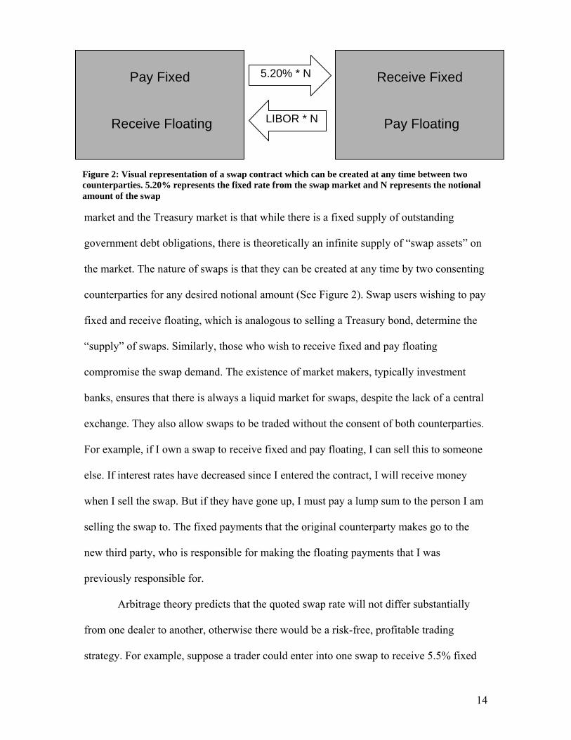
Figure 2: Visual representation of a swap contract which can be created at any time between two counterparties. 5.20% represents the fixed rate from the swap market and N represents the notional amount of the swap

market and the Treasury market is that while there is a fixed supply of outstanding

government debt obligations, there is theoretically an infinite supply of “swap assets” on

the market. The nature of swaps is that they can be created at any time by two consenting

counterparties for any desired notional amount (See Figure 2). Swap users wishing to pay

fixed and receive floating, which is analogous to selling a Treasury bond, determine the

“supply” of swaps. Similarly, those who wish to receive fixed and pay floating

compromise the swap demand. The existence of market makers, typically investment

banks, ensures that there is always a liquid market for swaps, despite the lack of a central

exchange. They also allow swaps to be traded without the consent of both counterparties.

For example, if I own a swap to receive fixed and pay floating, I can sell this to someone

else. If interest rates have decreased since I entered the contract, I will receive money

when I sell the swap. But if they have gone up, I must pay a lump sum to the person I am

selling the swap to. The fixed payments that the original counterparty makes go to the

new third party, who is responsible for making the floating payments that I was

previously responsible for.

Arbitrage theory predicts that the quoted swap rate will not differ substantially

from one dealer to another, otherwise there would be a risk-free, profitable trading

strategy. For example, suppose a trader could enter into one swap to receive 5.5% fixed

14

for 10 years and another to pay 5% fixed for 10 years. This trade is a financial free lunch;

traders can earn the guaranteed 0.5% spread between these two rates, regardless of what

happens in the market. They would execute this trade with as much money as possible,

including using leverage to their advantage. As money pours into this trade, however, the

5.5% rate will gradually decrease and the 5% rate will gradually increase until they

equilibrate and the arbitrage opportunity vanishes.

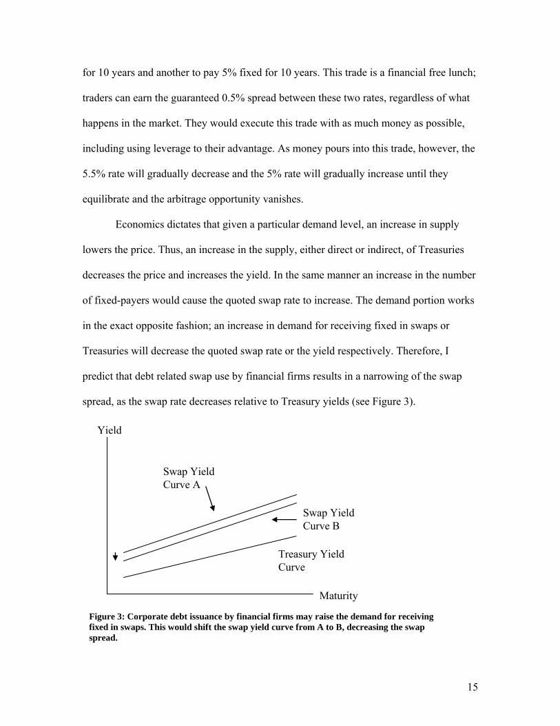
Economics dictates that given a particular demand level, an increase in supply

lowers the price. Thus, an increase in the supply, either direct or indirect, of Treasuries

decreases the price and increases the yield. In the same manner an increase in the number

of fixed-payers would cause the quoted swap rate to increase. The demand portion works

in the exact opposite fashion; an increase in demand for receiving fixed in swaps or

Treasuries will decrease the quoted swap rate or the yield respectively. Therefore, I

predict that debt related swap use by financial firms results in a narrowing of the swap

spread, as the swap rate decreases relative to Treasury yields (see Figure 3).

Figure 3: Corporate debt issuance by financial firms may raise the demand for receiving fixed in swaps. This would shift the swap yield curve from A to B, decreasing the swap spread.

Maturity

Yield

Treasury Yield Curve

Swap Yield Curve A

Swap Yield Curve B

15

Typical market events, such as economic data releases, tend to cause price

movem

the

yield cu

ment

d

,

crease

n

ents of approximately equal magnitude in the Treasury market and the swap

market. Therefore, we must examine some essential differences between the two markets

which drive the relative supply and demand and therefore the swap spread. Cortes (2003)

identifies a number of different explanatory variables that affect the swap spread. This

paper tests whether corporate debt issuance also helps determine the swap spread.

Cortes’ regression includes data reflecting budget expectations, the slope of

rve, the “on/off spread”, implied volatility from the equity market, and the

effective duration of mortgage backed securities. There is also a medium run adjust

variable which “accounts for the persistent deviations in swap spreads.” A decrease in the

budget expectations of the government (i.e. a deficit) would tighten the swap spread, as

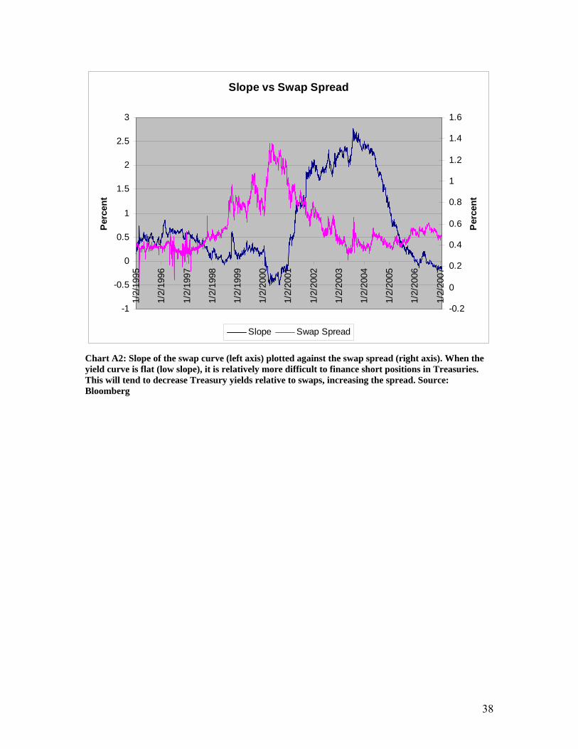
the supply of Treasuries increases relative to swaps. Empirically, the slope of the yield

curve is inversely related to swap spreads. This may stem from the fact that in an inverte

yield curve environment, financing a short position in Treasuries through the repurchase,

or repo, market becomes relatively more expensive. Thus there is a relative decrease in

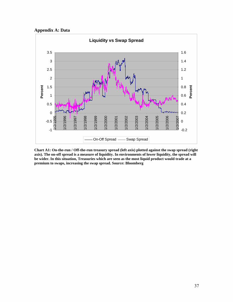
supply of Treasuries. The on/off spread is the difference in yield between the most liquid

on-the-run government bonds and less frequently traded off-the-run bonds. This spread

primarily reflects the liquidity premium other authors have identified as a driver of swap

spreads. Despite the growth in the swap market, people may still tend to view the

government bond market as the most liquid, so an increase in the on/off spread (de

in liquidity) should widen the swap spread as demand for bonds increases relative to

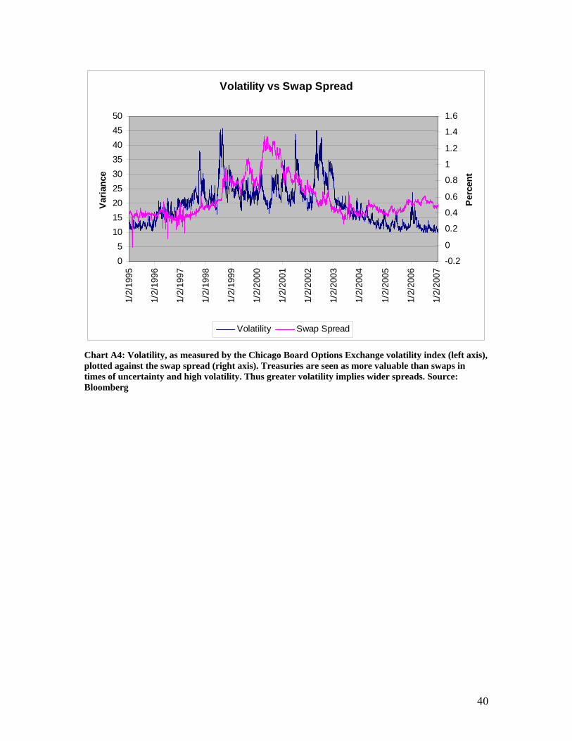
swaps. Government bonds are also considered extremely secure investments so that

demand may be boosted by a “flight-to-quality” in risky or uncertain periods. Thus a

16

increase in volatility expectations, as measured by the VIX, would increase the swap

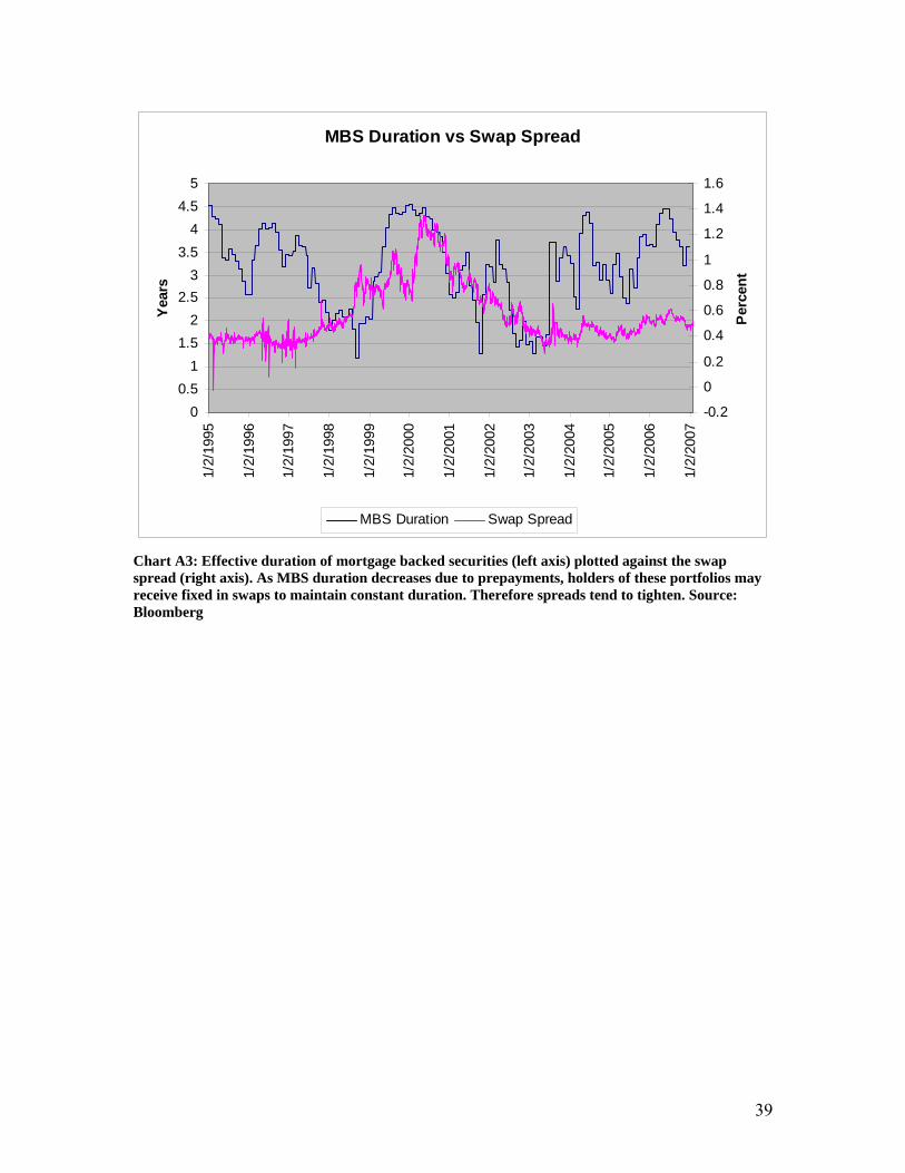
spread7. The effective duration of mortgage backed securities affects swap spreads

primarily because holders of mortgage portfolios, like corporations, have become m

active in using the swap market to manage their interest rate exposure. For example, in a

falling interest rate environment, more and more homeowners will refinance their

mortgages, shortening the duration of these portfolios. In order to maintain a consta

duration, portfolio managers may choose to receive fixed in swaps, which would narro

the swap spread. Since all of these variables affect the relative pricing of swaps and

Treasuries, I should include them in my model of swap spreads.

Cortes finds that the coefficients on slope, implied volatil

ore

nt

w

ity, effective duration of

mortga

I

ge backed securities, and the medium run adjustment variable are all significant

and obtains an R-squared value of 0.40. The form of my regressions will be similar, but

will add a variable that quantifies the issuance of debt by financial corporations and test

to see whether its coefficient is statistically significant. I will also include a variable that

measures LIBOR spreads since they are the fundamental driver of swap spreads.

7 The VIX is an index which tracks the “implied volatility” of the stock market. All other things equal, options are more valuable in a high volatility environment. Therefore if options prices are high, the VIX will also be at an elevated level, reflecting market expectations that large price swings may lie ahead.

17

IV. Data

I have obtained time series data for market variables which will allow me to

measure the factors which influence swap spreads. This data set was collected using

Bloomberg, a service that is a primary source of information for many market

professionals and is regarded as very reliable. In addition to including variables which

have been shown as significant in affecting swap spreads, my data set also contains an

index of financial debt issuance that enables me to test for the effect of corporate swap

use on swap spreads. The time series range from May 31, 1998 to January 25, 2007 and

include 2,284 daily price observations. I use the price of the last trade on each day.

As discussed in the previous section, there are numerous market factors which can

affect swap spreads8. The interest rate variables collected are 3 month LIBOR, the yield

on 3 month Treasury Bills, the 10 year swap rate, the yield of the on-the-run 2 and 10

year U.S. Treasuries9 and a Merrill Lynch index which tracks the yield of a basket of

“off-the-run” Treasuries with maturities ranging from 9.5 to 11 years. From this

fundamental group, I define the actual variables to be used in the regression as shown in

Table 1.

Regression Variable DefinitionSwap Spread 10 Year Swap Rate - 10 Year On The Run Treasury YieldOn/Off Spread 10 Year Off the Run Yield - 10 Year On the Run YieldSlope 10 Year Treasury Yield - 2 Year Treasury YieldLIBOR/T-Bill Spread 3 Month LIBOR - 3 Month T-Bill Yield

Table 1: Definition of interest rate variables used in the regression

8 See Section III for a complete list of these factors, their definitions, and reasoning for how they affect swap spreads. 9 These yields are obtained from Merrill Lynch indices which track the on-the-run Treasuries. The use of a separate index is necessary because Bloomberg contains the yield of the current 10 year note only back until the date when it first became on-the-run, which is typically less than 3 years. The indices are superior to Constant Maturity Treasury (CMT) yields because it reflects prices of actual securities whereas CMT is a synthetic measure.

18

One disadvantage of these definitions is that they are quite restrictive. Not all

firms will hedge with 10 year swaps, especially if the debt matures in less than 10 years.

As a result, even if a firm hedges its debt issuance using swaps, there may be no effect on

the ten year swap spread. But because precisely matching swap spreads with debt

issuance would be extremely difficult, I choose to use the 10 year swap spread because it

is a widely traded rate. In addition, there is a possibility that when a corporation hedges at

a certain point along the swap curve, other points on the curve could also tighten.

Imagine a firm receiving fixed in a seven year swap. The counterparty to this swap is

likely a dealer who may wish to hedge their newly acquired exposure to paying fixed by

receiving fixed. Depending on their market outlook and current positions, however, they

may hedge this exposure by receiving fixed at another maturity along the swap curve,

including the 10 year bucket, which would narrow the swap spread at that maturity.

Other market variables which I have obtained include the Chicago Board Options

Exchange volatility index (VIX), a Citigroup index which measures the effective duration

of mortgage backed securities, and a Bloomberg survey of economists’ expectations for

the monthly budget release by the U.S. Treasury. The last two sets are only computed

monthly, so they only have 104 observations. In addition, the budget expectations survey

may not be the best measure because it is based on short term expectations. Thus changes

in values recorded by this survey may not necessarily correspond with an altered market

view of future U.S. Treasury debt issuance, which is what impacts swap spreads.

Basic statistics for these time series can be found in Table 2. Graphs which

compare the swap spread to various independent variables are located in the Data

Appendix at the end of this paper. Note that the LIBOR/T-Bill spread is typically positive

19

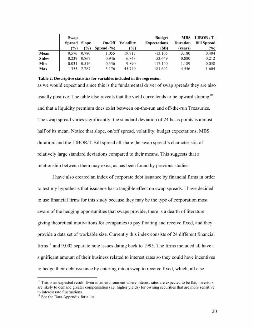
as we would expect and since this is the fundamental driver of swap spreads they are also

usually positive. The table also reveals that the yield curve tends to be upward sloping10

and that a liquidity premium does exist between on-the-run and off-the-run Treasuries.

The swap spread varies significantly: the standard deviation of 24 basis points is almost

half of its mean. Notice that slope, on/off spread, volatility, budget expectations, MBS

duration, and the LIBOR/T-Bill spread all share the swap spread’s characteristic of

relatively large standard deviations compared to their means. This suggests that a

relationship between them may exist, as has been found by previous studies.

I have also created an index of corporate debt issuance by financial firms in order

to test my hypothesis that issuance has a tangible effect on swap spreads. I have decided

to use financial firms for this study because they may be the type of corporation most

aware of the hedging opportunities that swaps provide, there is a dearth of literature

giving theoretical motivations for companies to pay floating and receive fixed, and they

provide a data set of workable size. Currently this index consists of 24 different financial

firms11 and 9,002 separate note issues dating back to 1995. The firms included all have a

significant amount of their business related to interest rates so they could have incentives

to hedge their debt issuance by entering into a swap to receive fixed, which, all else

Swap Spread

(%)Slope

(%)On/Off

Spread (%)Volatility

(%)

Budget Expectations

($B)

MBS Duration

(years)

LIBOR / T-Bill Spread

(%)Mean 0.576 0.780 1.055 19.717 -13.105 3.180 0.404Stdev 0.239 0.867 0.946 6.848 53.649 0.880 0.212Min -0.031 -0.516 -0.336 9.890 -117.140 1.189 -0.058Max 1.355 2.787 3.176 45.740 181.692 4.556 1.604

Table 2: Descriptive statistics for variables included in the regression

10 This is an expected result. Even in an environment where interest rates are expected to be flat, investors are likely to demand greater compensation (i.e. higher yields) for owning securities that are more sensitive to interest rate fluctuations. 11 See the Data Appendix for a list

20

equal, would decrease swap spreads. Like the above data series, the issuance data was

obtained from Bloomberg. I have also separated the firms into three separate categories

based on classifications by Yahoo! Finance. The categories are Investment Brokerage,

Regional and Money Center Banks, and Other Financial Firms. This will allow me to

determine whether certain subgroups of financial firms have different effects on swap

spreads.

For each security issued I gather the date that the issuance was announced, the

actual date of issuance, the maturity date, and the notional amount issued. In order to

properly account for the difference between $2B of debt maturing in two years and $2B

of debt maturing in 30 years, I have obtained a set of duration weights given certain

assumptions about the bonds (see Data Appendix). I multiply the amount issued (in

millions) by the duration to obtain the duration-weighted amount issued and sum these

amounts on each day to obtain the time series index of financial debt issuance. One

weakness of this data is that it is only a proxy for the actual amount these firms use swaps

to hedge their issuance. The extent to which they use swaps likely varies over time.

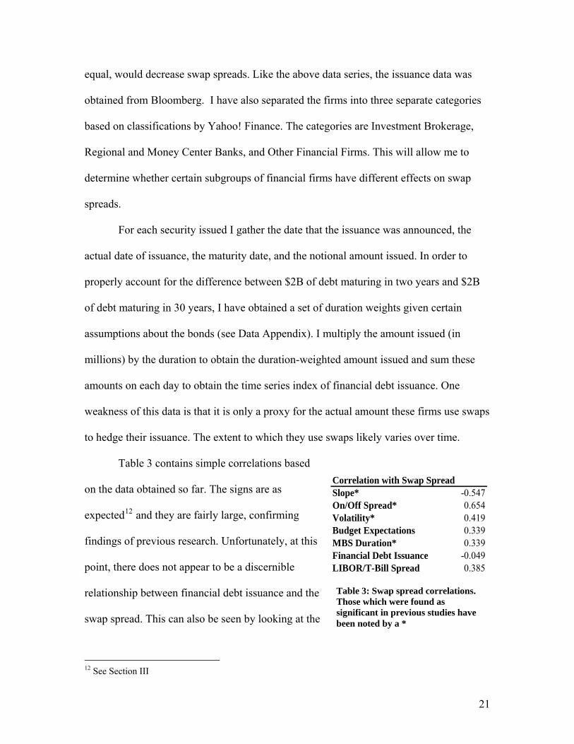
Table 3 contains simple correlations based

on the data obtained so far. The signs are as

expected12 and they are fairly large, confirming

findings of previous research. Unfortunately, at this

point, there does not appear to be a discernible

relationship between financial debt issuance and the

swap spread. This can also be seen by looking at the

Table 3: Swap spread correlations. Those which were found as significant in previous studies have been noted by a *

Correlation with Swap SpreadSlope* -0.547On/Off Spread* 0.654Volatility* 0.419Budget Expectations 0.339MBS Duration* 0.339Financial Debt Issuance -0.049LIBOR/T-Bill Spread 0.385

12 See Section III

21

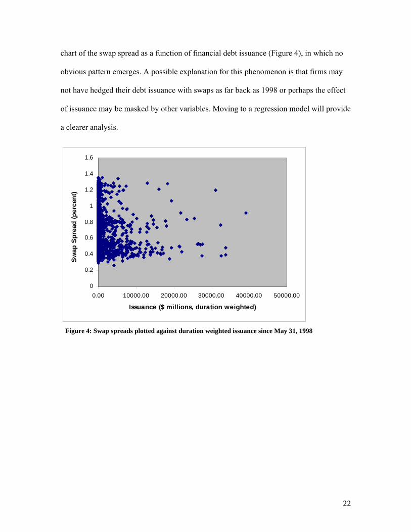
chart of the swap spread as a function of financial debt issuance (Figure 4), in which no

obvious pattern emerges. A possible explanation for this phenomenon is that firms may

not have hedged their debt issuance with swaps as far back as 1998 or perhaps the effect

of issuance may be masked by other variables. Moving to a regression model will provide

a clearer analysis.

Figure 4: Swap spreads plotted against duration weighted issuance since May 31, 1998

0

0.2

0.4

0.6

0.8

1

0.00 10000.00 20000.00 30000.00 40000.00 50000.00

Issuance ($ millions, duration weighted)

Swap

Spr

ead

(per

cen

1.2

1.4

1.6

t)

22

V. Empirical Specifications and Findings

As discussed in previous sections, I will attempt to determine the significance and

size of various market factors on the swap spread. My regression is similar to ones

performed in the past except that it is the first to explicitly include financial debt issuance

as a potential explanatory variable. The general form of my regressions is as follows13:

Swap Spreadt = β0 + β1 * Financial Debt Issuancet + β2 * Budget Expectationst

+ β3 * Slopet + β4 * On/Off Spreadt + β5 * Volatilityt

+ β6 * Duration of MBSt + β7 * LIBOR/T-Bill Spreadt

Instead of using first differences as has been done in previous studies, the regressions use

cross sectional data over time. This is done because unlike the other market variables,

issuance data varies widely over time. There can easily be $400 million of duration-

weighted issuance on one day, followed by none on the following day. While we expect a

tightening of swap spreads on the day of issuance, using first differences would lead to

accounting for the effect of “negative” $400 million of issuance on the second day on

swap spreads. Since it seems irrational for corporations to issue debt and hedge it on one

day, only to exit the hedge on the next day, I want to avoid capturing this effect. The

drawback of this approach is inputting the current levels of the various determinants

could result in a predicted swap spread that is quite different from the actual swap spread.

Despite this shortcoming, the model will still give predictions of the change in the

swap spread given a change in one of the independent variables, assuming that all the

other variables stay the same. For example, the coefficient β1 will allow market

participants to determine, on average, how much swap spreads move given a certain level

of issuance. In general, the results of the regression will allow market participants to 13 Definitions of these variables and rationale for their place in the regression can be found in Section III

23

analyze how the swap spread moves in response to a variety of factors and adjust their

investment decisions based on their views. Consider a simple example in which they

observe a change in the slope of the yield curve in the market but all the other factors

remain the same. Knowledge of the coefficient β3 will tell them how much, and in what

direction, the swap spread has historically moved in response to variations in slope. Then,

if there is a deviation between the actual and expected behavior of the swap spread, they

could decide to put on a trade. If financial debt issuance is indeed a determinant of swaps,

its inclusion should make the regression a better model for the behavior of swap spreads.

Table 4 above summarizes the expected signs on the various coefficients.

One weakness of the model is the use of the current LIBOR/T-Bill spread as an

explanatory variable for the current swap spread. In reality, it is expectations of future

LIBOR/T-Bill spreads that drive the swap spread. Therefore in its current specification,

the model assumes that the current level of LIBOR/T-Bill spreads is the best predictor of

future LIBOR/T-Bill spreads.

Another concern is the potential existence of reverse causality between corporate

debt issuance and swap spreads which could result in biased coefficients. The idea is that

corporate debt issuance not only has an effect on swap spreads, but swap spreads may in

Coefficient Variable Expected Signß1 Financial Debt Issuance -ß2 Budget Expectations +ß3 Slope -ß4 On/Off Spread +ß5 Volatility +ß6 Duration of MBS +ß7 LIBOR/T-Bill Spread +

Table 4: Expected signs on independent variables. Explanation of the variables and reasoning for the expected signs can be found in Section III

24

turn influence the timing and amount of corporate debt issuance. There are a number of

problems, however, which make such a scenario unlikely. Regardless of the level of swap

spreads, entering into a swap to receive fixed and pay floating has a net present value of

zero. Since the value of a corporation’s hedging tool does not change with swap spreads,

it is hard to imagine that they will change their issuance behavior based on swap spreads.

Corporations are also unlikely to have a view on the path of swap spreads which is more

accurate than market consensus so they should not be basing their financing decisions on

whether they believe swap spreads are relatively high or low.

This consideration, though, gives rise to the idea that corporate debt issuance is

not a completely independent variable. It is highly likely that the amount of issuance

depends on the level of interest rates because corporations are more prone to issue debt in

a period of low interest rates and cheap financing. To account for this possibility I include

the level of interest rates, as measured by the rate on the ten year Treasury note, in the

regression. This specification is not perfect, however, because the actual rate that

corporations pay on their debt also depends on corporate bond spreads over Treasuries,

but I was not able to obtain an appropriate data series to measure this factor.

I have run a number of different regressions, using different measures for the

amount of financial debt issuance to test my various research questions. One set of

regressions uses the date when the debt was actually brought to market (“Issuance Date”).

The “Announce Date” regressions account for the possibility that swap spreads could

tighten upon the announcement of future issuance, rather than at the time it is issued. This

may occur because people may anticipate swap spreads tightening with future issuance

and put on a trade to profit from that tightening. The actual act of executing such a trade

25

will tend to tighten swap spreads. Since the swap spread I have measured is the ten year

swap spread, it may be reasonable to assume that those issuing debt with maturities less

than ten years will not hedge with ten year swaps and therefore there will be no effect on

this particular swap spread. Thus another regression includes only debt issues with

maturities of 10 years or more. Finally, since the swap market is relatively young,

financial firms may have only recently started hedging their issuance with swaps. I have

run regressions using two separate start dates: May 31, 1998 and January 1, 2004.

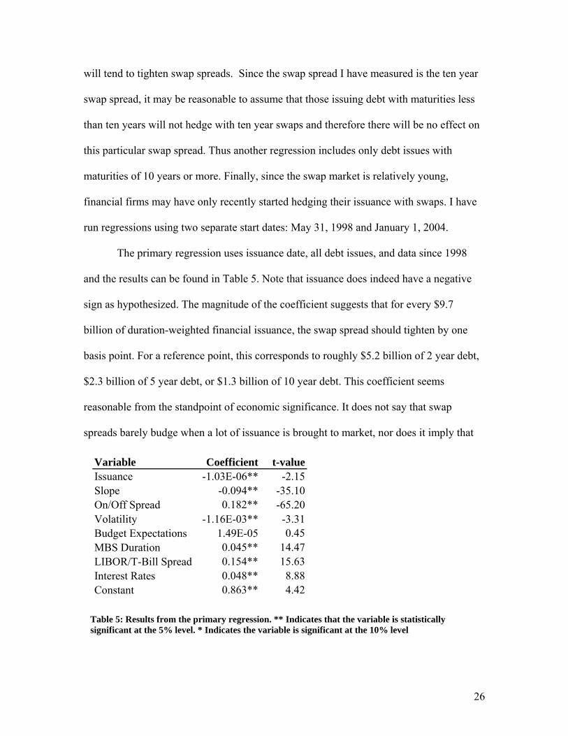
The primary regression uses issuance date, all debt issues, and data since 1998

and the results can be found in Table 5. Note that issuance does indeed have a negative

sign as hypothesized. The magnitude of the coefficient suggests that for every $9.7

billion of duration-weighted financial issuance, the swap spread should tighten by one

basis point. For a reference point, this corresponds to roughly $5.2 billion of 2 year debt,

$2.3 billion of 5 year debt, or $1.3 billion of 10 year debt. This coefficient seems

reasonable from the standpoint of economic significance. It does not say that swap

spreads barely budge when a lot of issuance is brought to market, nor does it imply that

Table 5: Results from the primary regression. ** Indicates that the variable is statistically significant at the 5% level. * Indicates the variable is significant at the 10% level

Variable Coefficient t-valueIssuance -1.03E-06** -2.15Slope -0.094** -35.10On/Off Spread 0.182** -65.20Volatility -1.16E-03** -3.31Budget Expectations 1.49E-05 0.45MBS Duration 0.045** 14.47LIBOR/T-Bill Spread 0.154** 15.63Interest Rates 0.048** 8.88Constant 0.863** 4.42

26

swap spreads experience huge variation every time a corporation decides to issue debt.

The 95% confidence interval runs from -1.97e-06 to -9.13e-08. These two values

correspond with a 1 basis point tightening for $5.1 billion and $11.0 billion of duration

weighted issuance respectively. The coefficient is statistically significant at the 5% level.

The regression also finds all the other variables except for budget expectations are

statistically significant. This may confirm earlier suspicions that the measure of budget

expectations used is not valid for this study. The coefficients on slope and on/off spread

imply that a 10 basis point steepening of the yield curve results in swap spreads that are

tighter by approximately one basis point and a five basis point increase in the “liquidity

premium” causes swap spreads to widen by one basis point. These results bear moderate

resemblance to Cortes’s earlier study because he found that slope, volatility, and duration

of mortgage backed securities were all statistically significant. The only coefficient

whose sign differs from expectations is volatility, but its coefficient is not very

economically significant. It suggests that an extremely large 10 point increase in

volatility as measured by the VIX would result in swap spreads widening by one basis

point. While the hypothesis was that investors may view Treasuries as a “flight-to-safety”

instrument in times of high volatility (LTCM Crisis in 1998, September 11, 2001) so that

swap spreads widen as volatility increases, the regression does not support this theory.

Perhaps one reason is that any increased risk to the banking system that investors

perceive is captured in the LIBOR/T-Bill spread. Alternatively, these events could be so

rare that their effects are minimized when examining long term averages.

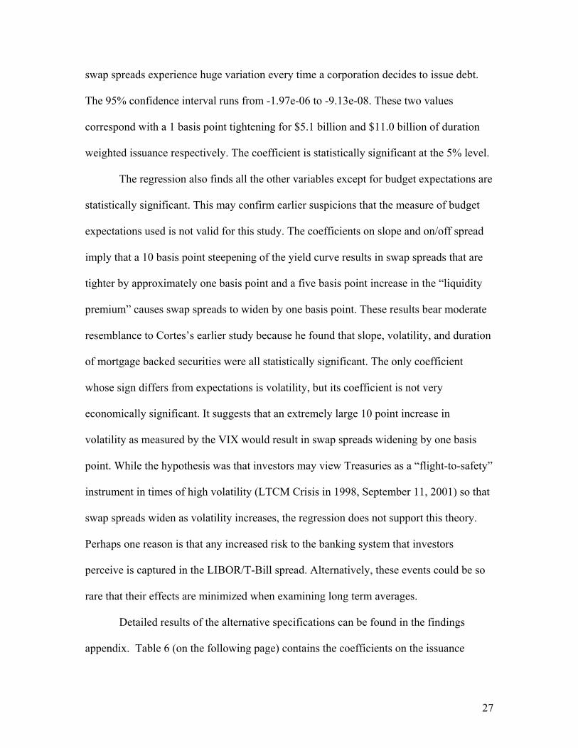
Detailed results of the alternative specifications can be found in the findings

appendix. Table 6 (on the following page) contains the coefficients on the issuance

27

Regression Coefficient t-value p-valueIssuance Date -1.03E-06** -2.15 0.03Issuance Date (2004) -1.52E-07 -0.64 0.52Announce Date -1.31E-06** -2.68 0.01Announce Date (2004) -1.63E-07 -0.69 0.49Issuance Date (10+ years) -8.82E-07 -1.50 0.13Issuance Date (10+ years, 2004) -9.54E-08 -0.34 0.73Announce Date (10+ years) -1.22E-06** -2.07 0.04Announce Date (10+ years, 2004) -2.20E-07 -0.81 0.42Investment Brokerage (Issuance Date) -1.10E-06 -1.21 0.23Regional / Money Center Banks (Issuance Date) -1.02E-06 -1.62 0.11Other Financial (Issuance Date) -2.86E-06 -1.29 0.20Investment Brokerage (Announce Date) -1.86E-06** -2.03 0.04Regional / Money Center Banks (Announce Date) -1.00E-06* -1.65 0.10Other Financial (Announce Date) -2.79E-06 -1.24 0.22Issuance Date (Monthly) -5.40E-07 -1.26 0.21Announce Date (Monthly) -4.21E-07 -1.01 0.31

Table 6: Coefficients on issuance measure for a number of different specifications measure for the different regressions. In general, the results align with the results of the

main regression in that the coefficient is always negative with a magnitude of around -

1E-06. The coefficient is statistically significant in four of the sixteen regressions at the

5% level and one additional regression at the 10% level.

A number of other observations can be made from the results in Table 6. First

note the difference in coefficient and significance in the regressions with data from 1998

to today and those with data from 2004 to today. In each of the four cases the magnitude

of the coefficient decreases and in the three cases where it was previously statistically

significant it turns statistically insignificant. This runs counter to the intuition which says

that as more and more firms become more aware of the hedging opportunities with

swaps, they will tend to hedge more which will increase the effect of issuance on the

swap spread. A trivial cause for this could be that in 1998 financial firms were just as

knowledgeable about swaps as they were in 2004 and are in 2007. Another possible

explanation for this phenomenon is that as the swap market has matured, transactions of

similar size have less of an effect on the overall market price. In other words, the market

28

can now “absorb” larger amounts of issuance without needing to adjust the price as much

as before.

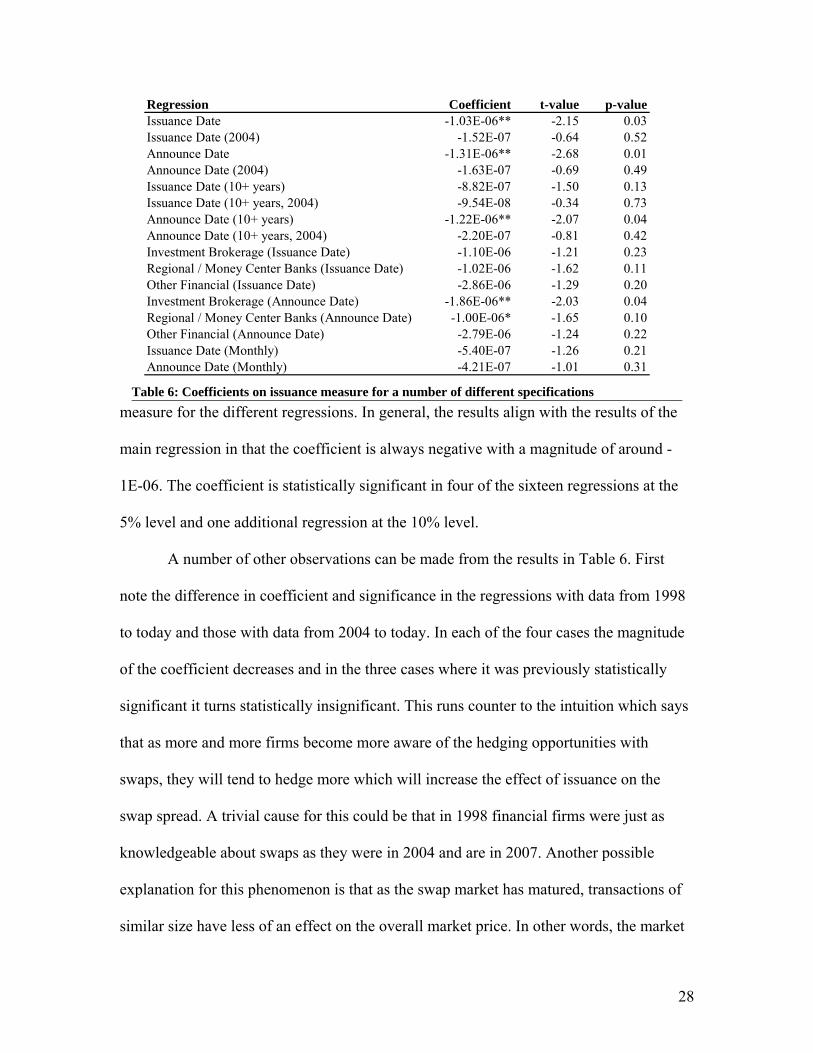
Another interesting finding is that swap spreads tend to tighten on both the

issuance date and the announce date when looking at the financial firms as one group.

This finding suggests another regression which regresses the swap spread on both

issuance by issue date and issuance by announce date. The results of these regressions are

contained in Table 7. Both measures of issuance remain statistically significant, though

the announce date coefficient is slightly larger. These findings mesh well with the theory

that some tightening will occur on the announce date, presumably caused by market

participants anticipating future hedging, followed by the actual tightening on the date the

new debt is issued.

No obvious claims can be made from the regressions containing different types of

firms on the issuance date, but there are noticeable differences on the announce date.

There is a statistically significant tightening for both the investment brokerages and the

regional/money center banks at the 5% and 10% level respectively, but the effect is not

Variable Coefficient t-valueIssuance (Issue Date) -9.47E-07** -1.97Issuance (Announce Date) -1.24E-06** -2.53Slope -0.094** -35.15On/Off Spread 0.182** 65.27Volatility -1.17E-03** -3.36Budget Expectations 1.96E-05 0.58MBS Duration 0.045** 14.46LIBOR/T-Bill Spread 0.153** 15.56Interest Rates 0.048** 8.87Constant 0.082** 4.58

Table 7: Regression containing both the issuance and the announce date since 1998

29

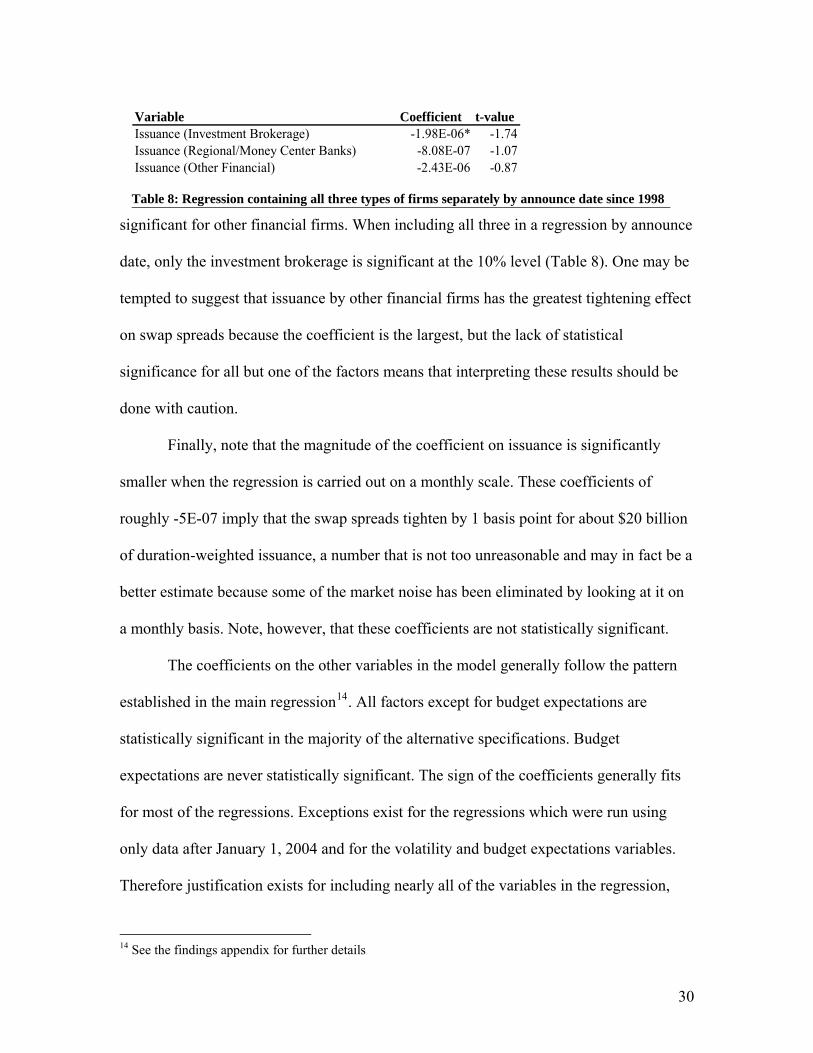
significant for other financial firms. When including all three in a regression by announce

date, only the investment brokerage is significant at the 10% level (Table 8). One may be

tempted to suggest that issuance by other financial firms has the greatest tightening effect

on swap spreads because the coefficient is the largest, but the lack of statistical

significance for all but one of the factors means that interpreting these results should be

done with caution.

Finally, note that the magnitude of the coefficient on issuance is significantly

smaller when the regression is carried out on a monthly scale. These coefficients of

roughly -5E-07 imply that the swap spreads tighten by 1 basis point for about $20 billion

of duration-weighted issuance, a number that is not too unreasonable and may in fact be a

better estimate because some of the market noise has been eliminated by looking at it on

a monthly basis. Note, however, that these coefficients are not statistically significant.

The coefficients on the other variables in the model generally follow the pattern

established in the main regression14. All factors except for budget expectations are

statistically significant in the majority of the alternative specifications. Budget

expectations are never statistically significant. The sign of the coefficients generally fits

for most of the regressions. Exceptions exist for the regressions which were run using

only data after January 1, 2004 and for the volatility and budget expectations variables.

Therefore justification exists for including nearly all of the variables in the regression,

Variable Coefficient t-valueIssuance (Investment Brokerage) -1.98E-06* -1.74Issuance (Regional/Money Center Banks) -8.08E-07 -1.07Issuance (Other Financial) -2.43E-06 -0.87

Table 8: Regression containing all three types of firms separately by announce date since 1998

14 See the findings appendix for further details

30

though a future study may want to obtain a data series for budget expectations which

more accurately represents the long term funding needs of the U.S. Treasury.

31

VI. Conclusions

This paper set out to discover whether corporate use of swaps has an identifiable

effect on swap spreads. The results section contains details showing that corporate

issuance does appear to be associated with a tightening of swap spreads, though the result

is not always statistically significant. Practical interpretation of the coefficients obtained

in the regressions is difficult, even in the cases where the results are statistically

significant. Knowing that swap spreads should tighten by about a basis point for duration

weighted issuance between $5.1 billion and $11.0 billion is not a very narrow estimate.

Also note that, contrary to expectations, the effect of issuance on swap spreads may be

decreasing over time as the swap market grows even larger.

Despite the apparent negative relationship between financial debt issuance and

swap spreads, readers must be cautious in making any broad conclusions regarding

financial corporations’ swap use since large assumptions have been made about using

their issuance as a proxy for their swap use and about their use of ten year swaps, in

particular, to hedge the issuance. While a general pattern may exist, specific methods of

implementing swap hedges probably vary widely amongst financial firms.

In a similar manner, the dynamics of the relationship between corporate debt

issuance and swap spreads are constantly changing. As more people in the market

become aware of the spread tightening that may occur with issuance, expectations and

anticipation of future issuance may begin driving spreads more than actual issuance.

Indeed, if corporations end up issuing less than the market expects, swap spreads could

potentially widen on the issuance date. Future studies could investigate whether swap

spreads at time t are actually dependent on issuance at some point after time t. Another

32

factor to consider is that the negative relationship is based on the idea that financial firms

wish to borrow at floating rates, but the market demand for floating rate debt is rather

limited so that they must issue fixed rate debt and swap into floating rate debt. If

conditions change and market demand for floating rate debt increases, these firms are

likely to skip the intermediate step of using the swap market and simply issue floating

rate debt.

A potential flaw of this study is its limited scope. Corporate swap use is certainly

not limited to financial corporations. Favorable interest rate environments in which

financials choose to issue debt may also coincide with non-financial corporations issuing

debt and swapping into paying fixed rather than swapping into receiving fixed. This

would have an opposing, widening effect on swap spreads, making the net effect

ambiguous. The actual performance of swap spreads would then depend on the

probability that financial firms use swaps alongside their debt issuance compared to the

probability that non-financial firms use them and the relative magnitudes of the debt

issuance by the two types of corporations.

Another implication of this study is that more theoretical work may need to be

pursued to more clearly understand the rationale for corporations to enter into swaps to

receive fixed. Much of the literature currently focuses on the decision for firms to pay

fixed in swaps. Since this paper finds, however, that financial debt issuance tends to have

a tightening effect on swap spreads, a more rigorous framework may need to be

developed to fully explain why financial firms engage in their current behavior.

Finally, this paper further adds to a growing body of empirical work which

concludes that corporate use of swaps is fairly prevalent. This confirms that swaps are not

33

simply another clever financial innovation created for Wall Street to speculate on interest

rates, but that they are quite practical for those on Main Street too.

34

References

Bank for International Settlements. (2006). BIS Quarterly Review September 2006:

International banking and financial market developments. Basel, Switzerland.

Barrett, S., & Marine, C. (2006, September 7). Investment-grade market booms. The Wall

Street Journal, pp. C6.

Bicksler, J., & Chen, A.H. (1986). An Economic Analysis of Interest Rate Swaps. The

Journal of Finance, 41(3), 645-656.

Duffie, D., & Huang, M. (1996). Swap rates and credit quality. The Journal of Finance,

51(3), 921-950.

Cortes, F. (2003). Understanding and modeling swap spreads. Bank of England Quarterly

Bulletin, 43(4), 407-416.

Fehle, F. (2003). The components of interest rate swap spreads: Theory and international

evidence. The Journal of Futures Markets, 23(4), 347-387.

Li, H., & Mao, C. X. (2003). Corporate use of interest rate swaps: Theory and evidence.

Journal of Baking & Finance, 27(8), 1511-1538.

Litzenberger, R.H. (1992). Swaps: Plain and Fanciful. Journal of Finance, 47(3), 831-

851.

Liu, J., Longstaff, F. A., & Mandell, R.E. (2002). The Market Price of Credit Risk: An

Empirical Analysis of Interest Rate Swap Spreads. NBER Working Paper Series.

Retrieved September 12, 2006, from http://www.nber.org/papers/w8990.

Simkins, B.J., & Rogers, D.A. (2006). Asymmetric information and credit quality:

Evidence from synthetic fixed-rate financing. The Journal of Futures Markets,

26(6)

35

Titman, S. (1992). Interest Rate Swaps and Corporate Financing Choices. Journal of

Finance, 47(4), 1503-1517.

Visvanathan, G. (1998). Who Uses Interest Rate Swaps? A Cross-Sectional Analysis.

Journal of Accounting, Auditing & Finance, 13(3), 173-201.

36

Appendix A: Data

Liquidity vs Swap Spread

-1

-0.5

0

0.5

1

1.5

2

2.5

3

3.51/

2/19

95

1/2/

1996

1/2/

1997

1/2/

1998

1/2/

1999

1/2/

2000

1/2/

2001

1/2/

2002

1/2/

2003

1/2/

2004

1/2/

2005

1/2/

2006

1/2/

2007

Per

cent

-0.2

0

0.2

0.4

0.6

0.8

1

1.2

1.4

1.6

Per

cent

On-Off Spread Swap Spread

Chart A1: On-the-run / Off-the-run treasury spread (left axis) plotted against the swap spread (right axis). The on-off spread is a measure of liquidity. In environments of lower liquidity, the spread will be wider. In this situation, Treasuries which are seen as the most liquid product would trade at a premium to swaps, increasing the swap spread. Source: Bloomberg

37

Slope vs Swap Spread

-1

-0.5

0

0.5

1

1.5

2

2.5

3

1/2/

1995

1/2/

1996

1/2/

1997

1/2/

1998

1/2/

1999

1/2/

2000

1/2/

2001

1/2/

2002

1/2/

2003

1/2/

2004

1/2/

2005

1/2/

2006

1/2/

2007

Perc

ent

-0.2

0

0.2

0.4

0.6

0.8

1

1.2

1.4

1.6

Perc

ent

Slope Swap Spread

Chart A2: Slope of the swap curve (left axis) plotted against the swap spread (right axis). When the yield curve is flat (low slope), it is relatively more difficult to finance short positions in Treasuries. This will tend to decrease Treasury yields relative to swaps, increasing the spread. Source: Bloomberg

38

MBS Duration vs Swap Spread

00.5

11.5

22.5

33.5

44.5

5

1/2/

1995

1/2/

1996

1/2/

1997

1/2/

1998

1/2/

1999

1/2/

2000

1/2/

2001

1/2/

2002

1/2/

2003

1/2/

2004

1/2/

2005

1/2/

2006

1/2/

2007

Yea

rs

-0.2

0

0.2

0.4

0.6

0.8

1

1.2

1.4

1.6

Per

cent

MBS Duration Swap Spread

Chart A3: Effective duration of mortgage backed securities (left axis) plotted against the swap spread (right axis). As MBS duration decreases due to prepayments, holders of these portfolios may receive fixed in swaps to maintain constant duration. Therefore spreads tend to tighten. Source: Bloomberg

39

Volatility vs Swap Spread

05

101520253035404550

1/2/

1995

1/2/

1996

1/2/

1997

1/2/

1998

1/2/

1999

1/2/

2000

1/2/

2001

1/2/

2002

1/2/

2003

1/2/

2004

1/2/

2005

1/2/

2006

1/2/

2007

Var

ianc

e

-0.2

0

0.2

0.4

0.6

0.8

1

1.2

1.4

1.6

Perc

ent

Volatility Swap Spread

Chart A4: Volatility, as measured by the Chicago Board Options Exchange volatility index (left axis), plotted against the swap spread (right axis). Treasuries are seen as more valuable than swaps in times of uncertainty and high volatility. Thus greater volatility implies wider spreads. Source: Bloomberg

40

Financial Debt Issuance vs Swap Spread

0.00

5000.00

10000.0015000.00

20000.00

25000.00

30000.0035000.00

40000.00

45000.00

1/2/

1995

1/2/

1996

1/2/

1997

1/2/

1998

1/2/

1999

1/2/

2000

1/2/

2001

1/2/

2002

1/2/

2003

1/2/

2004

1/2/

2005

1/2/

2006

1/2/

2007

$ (m

illio

ns)

-0.2

0

0.20.4

0.6

0.8

11.2

1.4

1.6

Perc

ent

Financial Debt Issuance Swap Spread

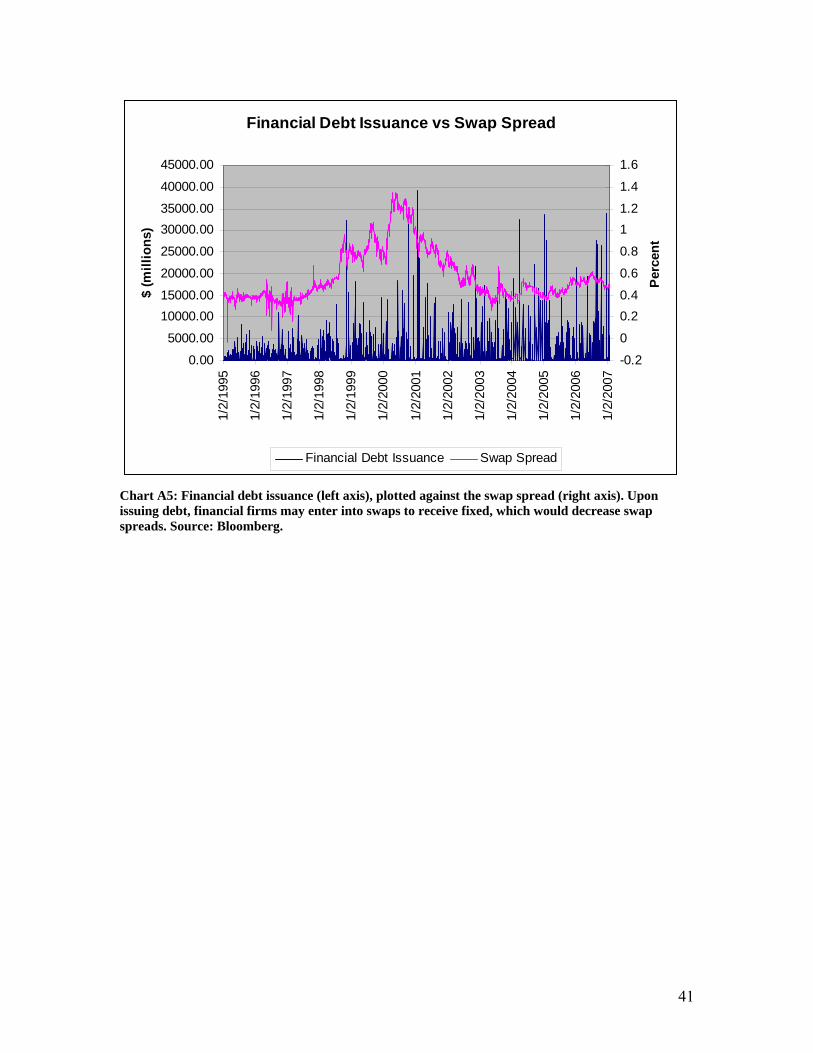
Chart A5: Financial debt issuance (left axis), plotted against the swap spread (right axis). Upon issuing debt, financial firms may enter into swaps to receive fixed, which would decrease swap spreads. Source: Bloomberg.

41

Financial FirmsTicker Firm Firm Type Category

BSC The Bear Stearns Companies Investment Brokerage AGS Goldman Sachs Group Investment Brokerage A

LEH Lehman Brothers Holdings Investment Brokerage AMER Merrill Lynch Investment Brokerage A

MS Morgan Stanley Investment Brokerage ABAC Bank of America Money Center Banks BBBT BB&T Corporation Regional Banks BBCS Barclays PLC Money Center Banks B

C Citigroup Regional Banks BCS Credit Suisse Group Money Center Banks BDB Deutsche Bank Money Center Banks B

JPM JPMorgan Chase Money Center Banks BKEY KeyCorp Money Center Banks BPNC PNC Financial Services Money Center Banks B

RY Royal Bank of Canada Money Center Banks BSTI SunTrust Money Center Banks B

UBS UBS AG Money Center Banks BUSB U.S. Bancorp Regional Banks BWB Wachovia Money Center Banks B

WFC Wells Fargo Money Center Banks BAXP American Express Credit Services CCFC Countrywide Financial Mortgage Investment CCOF Capital One Financial Credit Services CWM Washington Mutual Savings & Loans C

Table A1: Financial firms included in the index of financial debt issuance. The firms have been divided up into 3 categories: Investment Brokerage (A), Regional and Money Center Banks (B), and Other Financial (C).

Years Duration

1 0.96 2 1.86 3 2.71 5 4.26 7 5.65

10 7.44 12 8.47 15 9.80 20 11.55 30 13.83

Table A2: Duration weights assuming 6% coupon and bond priced at par. I fit a curve to these weights: the equation is Duration = (-.0127)*Years^2 + (0.8275)*Years + 0.3186. I use this curve to calculate durations, given the maturity and issue date of a bond.

42

Appendix B: Findings and Results

Issuance SlopeOn/Off Spread Volatility

Budget Expectations

MBS Duration

Libor-Tbill Spread Rates Constant

By IssuanceCoefficient -1.03e-06** -0.094** 0.182** -1.16e-03** 1.49e-05 0.045** 0.154** 0.048** 0.863**

t-value -2.15 -35.10 -65.20 -3.31 0.45 14.47 15.63 8.88 4.42

By Issuance (2004)Coefficient -1.52e-07 7.86e-03** -0.063** 1.79e-04** -8.75e-05** 0.041** 0.072** 0.071** -0.024

t-value -0.64 2.18 -6.72 3.44 -4.66 14.87 5.62 12.63 -1.09

By AnnounceCoefficient -1.31e-06** -0.094** 0.182** -1.17e-03** 1.72e-05 0.045** 0.154** 0.048** 0.080**

t-value -2.68 -35.11 65.23 -3.34 0.51 14.46 15.63 8.89 4.46

By Announce (2004)Coefficient -1.63e-07 7.89e-03** -0.063** 1.79e-03** -8.72e-05** .041** 0.072** 0.071** -0.024**

t-value -0.69 2.19 -6.72 3.44 -4.64 14.83 5.61 12.65 -1.11

By Issuance (10+ Yrs)Coefficient -8.82e-07 -0.094** 0.181** -1.14e-03** 1.38e-05 0.045** 0.154** 0.048** 0.078**

t-value -1.5 -35.08 65.14 -3.28 0.41 14.48 15.68 8.85 4.37

By Announce (10+ Yrs)Coefficient -1.22e-06** -0.094** 0.181** -1.15e-03** 1.51e-04 0.045** 0.154** 0.048** 0.079**

t-value -2.07 -35.10 65.15 -3.30 0.45 14.47 15.66 8.86 4.41

Investment Brokerage (Issuance)Coefficient -1.10e-06 -0.094** 0.182** -1.17e-03** 1.25e-05 0.045** 0.155** 0.048** 0.077**

t-value -1.21 -35.05 65.15 -3.33 0.37 14.44 15.71 8.90 4.32

Regional and Money Center Banks (Issuance)Coefficient -1.02e-06 -0.094** 0.182** -1.15e-03** 1.44e-05 0.045** 0.154** 0.048** 0.078**

t-value -1.62 -35.08 65.17 -3.28 0.43 14.47 15.63 8.89 4.36

Other Financial Firms (Issuance)Coefficient -2.08e-06 -0.094** 0.182** -1.16e-03** 1.23e-05 0.045** 0.154** 0.048** 0.077**

t-value -1.29 -35.06 65.17 -3.31 0.37 14.49 15.68 8.86 4.34

Investment Brokerage (Announce)Coefficient -1.86e-06** -0.094** 0.182** -1.17e-03** 1.37e-05 0.045** 0.155** 0.048** 0.078**

t-value -2.03 -35.07 65.19 -3.34 0.41 14.45 15.74 8.89 4.39

Regional and Money Center Banks (Announce)Coefficient -1.00e-06* -0.094** 0.182** -1.16e-03** 1.48e-05 0.045** 0.154** 0.048** 0.078**

t-value -1.65 -35.08 65.17 -3.31 0.44 14.45 15.63 8.91 4.35

Other Financial Firms (Announce)Coefficient -2.79e-06 -0.094** 0.182** -1.15e-03** 1.31e-05 0.045** 0.154** 0.048** 0.077**

t-value -1.24 -35.06 65.16 -3.30 0.39 14.50 15.68 8.86 4.34

Issuance (Monthly)Coefficient -5.40e-07 -0.106** 0.201** 1.11e-03 -2.34e-04 0.088** 0.180** -0.020 0.213**

t-value -1.26 -8.50 15.23 0.65 -1.53 5.01 3.97 -0.68 2.47

Announce (Monthly)Coefficient -4.21e-07 -0.106** 0.201** 1.15e-03 -2.20e-04 0.088** 0.181** -0.020 0.207**

t-value -1.01 -8.45 15.16 0.67 -1.43 5.02 3.99 -0.68 2.40

Table B1: Results of alternative specification regressions. ** represents statistical significance at the 5% level. * represents significance at the 10% level

43