


Languages
Pages
Legal

Numerical Methods in Civil Engineering, Vol. 2, No. 1, September. 2017
Numerical Methods in Civil Engineering
Controlling structures by inverse adaptive neuro fuzzy inference system
and MR dampers
M. Rezaiee-Pajand*, A. Baghban**
ARTICLE INFO
Article history:
Received:
January 2017.
Revised:
May 2017.
Accepted:
July 2017.
Keywords:
Control of structure;
semi-active control;
Adaptive Neuro Fuzzy
Inference System;
MR damper.
Abstract:
To control structures against wind and earthquake excitations, Adaptive Neuro Fuzzy
Inference Systems and Neural Networks are combined in this study. The control scheme consists
of an ANFIS inverse model of the structure to assess the control force. Considering existing
ANFIS controllers, which require a second controller to generate training data, the authors’
approach does not need another controller. To generate control force, active and semi-active
devices could be used. Since the active ANFIS inverse controller may not guarantee a
satisfactory response due to different uncertainties associated with operating conditions and
noisy training data, this paper uses MR dampers as semi-active devices to provide control
forces. To overcome the difficulty of tuning command voltage of MR dampers, a neural network
inverse model is developed. The effectiveness of the proposed strategy is verified and illustrated
using simulated response of the 3-story full-scale nonlinear benchmark building excited by
several earthquake records through computer simulation. Moreover, the recommended control
algorithm is validated using the wind-excited 76-story benchmark building equipped with MR
and TMD dampers. Comparing results with other controllers demonstrates that the proposed
method can reduce displacement, drift and acceleration, significantly.
1. Introduction
With the increasing studies in the field of structural
control, various control methods have been proposed.
Generally, these schemes can be divided into two groups.
The first one comprises control strategies that require
accurate mathematical formulation for the structural model.
Although structural models can be developed, there are
many sources of uncertainty, measurement noise and
nonlinearity that reduce effectiveness of control algorithms.
LQR, LQG, H2 and sliding model control techniques are
* Corresponding Author: Professor, Civil Engineering Department,
Ferdowsi University of Mashhad, Iran. Email: [email protected].
** PhD student., Civil Engineering Department, Ferdowsi University of
Mashhad, Iran. Email:[email protected].
some instances of this group. In recent years, there has been
a growing trend toward utilization of intelligent control as a
second group of control methods (Al-Dawod et al. 2004[1];
Pourzeynali et al. 2007[20]; Rezaiee-Pajand et al. 2009[21];
Karamodin et al. 2012[10]; Marinaki et al. 2015[16]; Park
& Ok 2015[19]). This group of controllers which does not
require an accurate mathematical model of structure
includes neural network and fuzzy control methods.
Fuzzy logic provides a Powerful tool for utilization of
human expert knowledge in complement to mathematical
knowledge. The main advantages of the fuzzy controller are:
(a) It is capable of handling the non-linear behavior of
the structures.
Dow
nloa
ded
from
nm
ce.k
ntu.
ac.ir
at 5
:05
+04
30 o
n M
onda
y Ju
ne 1
1th
2018
25
(b) It can tolerate uncertainties such as structural
uncertainties and assumed loading distribution.
(c) It is one of the few mathematical model-free
approaches for structural control.
(d) It can be adapted to new situations by modifying its
rules or membership functions.
Artificial Neural Network (ANN) controller is another
control method, which is associated with intelligent control
methods. ANN is a system that includes a number of similar
non-linear processing elements. These processing elements
operate in parallel and are arranged in patterns similar to the
patterns found in biological neural nets. The processing
elements or nodes are connected to each other by adjustable
weights. These weights will change in such a way to achieve
a desired input-output relationship. ANNs can be used for
time series prediction, classification, and control and
identification purposes. Several strategies have been
presented for structural control using ANNs (Jung et al.
2004[8]; Bani-Hani et al. 2006[2]; Lee et al. 2006[15];
Kumar et al. 2007[12]).
Adaptive-network-based fuzzy inference system
(ANFIS) is a very powerful approach for modeling complex
and nonlinear systems (Kadhim 2011[9]). It has the
advantages of learning capability of neural networks and
expert knowledge of fuzzy logic. ANFIS includes a fuzzy
inference system whose membership functions are
interactively adjusted according to a given set of input and
output data. Schurter & Roschke (2001)[22] and Gu &
Oyadiji (2008)[6] used ANFIS for control of structure. In
their approach, training data was generated using LQR and
LQG controllers, respectively. The disadvantage of training
ANFIS using other controllers is that, the trained ANFIS
controller works worse than the reference controllers, in
most situations. In best conditions, an ANFIS controller can
work as well as reference controllers.
Since the semi-active control combines the adaptability
associated with active control and the reliability associated
with passive control, it is generating great interest among
researchers in the field of structural control (Choi et al.
2004[3]; K-Karamodin et al. 2008[14]; Karamodin et al.
2012[10]; Kerboua et al. 2014[11]). The
magnetorheological (MR) damper is a device in this class
that generates force in response to velocity and applied
voltage. Because of the inherent nonlinear nature of this
device, one of the challenging aspects of utilizing this
technology is in the development of suitable control
algorithms. Several strategies have been developed for
control of MR dampers. Dyke et al. (1996)[4] developed a
semi-active clipped-optimal control algorithm to reduce the
response of structure with a MR damper. In their strategy,
the command voltage of the MR damper was tuned by a
linear optimal controller combined with a force feedback
loop. The command signal was adjusted at either zero or the
maximum level, depending on how the damper’s force
compared with the desired optimal control force. Choi et al.
(2004)[3] presented a semi-active fuzzy control strategy for
seismic response reduction using an MR damper. In their
approach, the output variable of the fuzzy controller was the
command voltage of MR damper. Karamodin et al.
(2008)[14] designed a neuro-predictive algorithm to predict
the voltage command of MR damper to provide the control
force determined by LQG controller.
In this paper, ANFIS based inverse model control is
developed for semi-active control of structures based on
acceleration feedback. This method is a straightforward
method to design a controller in which the controller is the
inverse of the plant. This approach only needs one learning
task to find the plant inverse and doesn’t require other
controllers to generate training data. Here, MR dampers are
selected as semi-active devices to provide control forces. To
set the command voltage of each MR damper in order to
provide the desired force determined by ANFIS controller,
an NN inverse model of MR damper is employed. The
effectiveness of proposed strategy is verified and illustrated
using simulated response of the 3-, and 76-story benchmark
buildings excited by various earthquake records and wind,
respectively. The results are compared with passive and
active control systems.
2. Benchmark Building Model
2. 1. 3-Story Benchmark Building
The nonlinear benchmark 3-story building used for this
study was defined by Ohtori et al. (2004)[17] in the problem
definition paper. The building is 11.89 m in height and 36.58
m by 54.87 m in the plan. The first three natural frequencies
of the 3-story benchmark evaluation model are: 0.99, 3.06,
and 5.83 Hz. Four historical ground motion earthquake
records (two far-field and two near-field) are selected for
study: El Centro (1940), Hachinohe (1968), Northridge
(1994) and Kobe (1995). Control actuators are located on
each floor of the structure to provide forces to adjacent
floors. Since the MR dampers capacity is limited to a
maximum force of 1,000 kN, three, two and two dampers are
used at the first, second and the third floors of the structure
respectively to provide the required larger forces. Three
sensors for acceleration measurements are employed for
feedback in the control system on the first, second and third
floors. Moreover, three sensors for velocity measurement
are used on the floors to determine the voltage of MR
dampers based on the command force.
During large seismic events, structural members can
yield, resulting in nonlinear response, behavior that may be
significantly different from a linear approximation. To
represent the nonlinear behavior, a bilinear hysteresis model
Dow
nloa
ded
from
nm
ce.k
ntu.
ac.ir
at 5
:05
+04
30 o
n M
onda
y Ju
ne 1
1th
2018
Numerical Methods in Civil Engineering, Vol. 2, No. 1, September. 2017
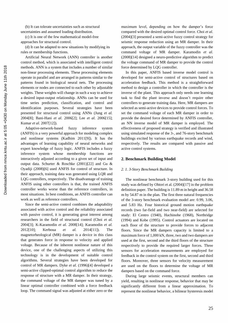
is used to model the plastic hinges (Fig. 1). These plastic
hinges, which are assumed to occur at the moment resisting
column-beam and column-column connections, introduce a
material nonlinear behavior of these structures.
To determine the time-domain response of such nonlinear
structures, the Newmark-β Time-step integration method
developed in MATLAB by Ohtori & Spencer (1999) [18] is
used. The incremental equations of motion for the nonlinear
structural system take the following form:
𝑀∆�̈� + 𝐶∆�̇� + 𝐾∆𝑈 = −𝑀𝐺∆𝑋�̈� + 𝑃∆𝑓 + ∆𝐹𝑒𝑟𝑟 (1)
where, M, C, and K are the mass, damping and stiffness
matrices of the building, ΔU is the incremental response
vector, G is a loading vector for the ground acceleration,
∆𝑋�̈� is the ground acceleration increment, P is a loading
vector for the ground forces, Δf is the incremental control
force and Δferr is the vector of the unbalanced forces.
Fig. 1: Bilinear hysteresis model for structural member bending.
2. 2. 76- Story Benchmark Building
The nonlinear benchmark 76-story building used for this
study was defined by Yang et al. (1999)[24] in the problem
definition paper. The building is a 76-story 306 meters
concrete office tower proposed for the city of Melbourne,
Australia. It is slender with a height to the width ratio of 7.3;
hence, this structure is wind sensitive. The first five natural
frequencies are 0.16, 0.765, 1.992, 3.790 and 6.395 Hz,
respectively. Damping ratios for the first five modes are
assumed to be 1% of critical for the proportional damping
matrix. A semi-active tuned mass damper (TMD) includes a
MR damper and an inertial mass of 500 tons that is installed
on the top floor. The mass is about 45% of the top-floor
mass, which is 0.327% of the total mass of the building. The
damper natural frequency is tuned to 0.16 Hz and its
damping ratio is set at 20%. The well-known Davenport
wind load spectrum, which has been used in the Canadian
design code, is used herein for along-wind loads. A sensor
for acceleration measurement is employed for feedback in
the control system on the 76th floor, and two sensors are
employed for velocity measurement on the 76th floor and
TMD to determine the voltage of MR damper based on the
control force.
3. MR Damper Model
An MR damper typically comprises of a hydraulic
cylinder, magnetic coils, and MR fluids that consist of
micrometer-sized magnetically polarizable particles floating
within oil-type fluids. In the presence of a magnetic field,
the particles polarize and provide an increased resistance to
flow. By altering the magnetic field, the desired behavior of
MR dampers can be earned. Since MR fluid can be changed
from a viscous fluid to a yielding solid within milliseconds,
and the resulting damping force can be notably large with a
low-power requirement, MR dampers are appropriate for
full-scale applications (Xu et al. 2000[23]).
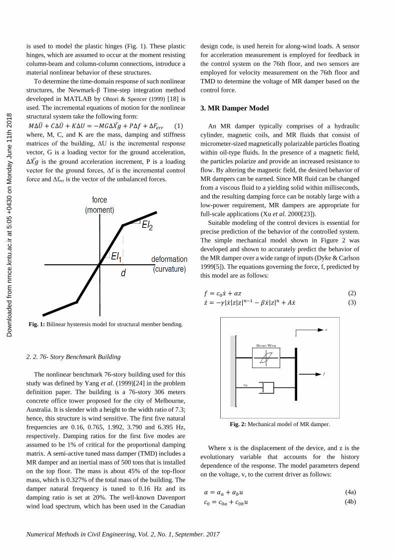
Suitable modeling of the control devices is essential for
precise prediction of the behavior of the controlled system.
The simple mechanical model shown in Figure 2 was
developed and shown to accurately predict the behavior of
the MR damper over a wide range of inputs (Dyke & Carlson
1999[5]). The equations governing the force, f, predicted by
this model are as follows:
𝑓 = 𝑐0�̇� + 𝛼𝑧 (2)
�̇� = −𝛾|�̇�|𝑧|𝑧|𝑛−1 − 𝛽�̇�|𝑧|𝑛 + 𝐴�̇� (3)
Fig. 2: Mechanical model of MR damper.
Where x is the displacement of the device, and z is the
evolutionary variable that accounts for the history
dependence of the response. The model parameters depend
on the voltage, v, to the current driver as follows:
𝛼 = 𝛼𝑎 + 𝛼𝑏𝑢 (4a)
𝑐0 = 𝑐0𝑎 + 𝑐0𝑏𝑢 (4b)
Dow
nloa
ded
from
nm
ce.k
ntu.
ac.ir
at 5
:05
+04
30 o
n M
onda
y Ju
ne 1
1th
2018
27
where u is given as the output of the first-order filter:
�̇� = −𝜂(𝑢 − 𝑣) (5)
Equation 5 is used to model the dynamics involved in
reaching theological equilibrium and in driving the
electromagnet in the MR damper (Dyke & Carlson 1999[5]).
This MR damper model is used in this study to model the
behavior of the MR damper. Selected parameters of the MR
damper are given in Table 1:
Table 1: MR damper parameters.
MR damper parameters
𝛼𝑎 1.0872e5 N/cm 𝐴 1.2
𝛼𝑏 4.9616e5 N/(cm V) 𝛾 3 cm-1
𝑐0𝑎 4.40 N s/cm 𝛽 3 cm-1
𝑐0𝑏 44.0 N s/(cm V) 𝜂 50 s-1
𝑛 1
These parameters are based on the identified model of an
MR damper tested at Washington University (Yi et al.
2001[25] & 2009[26]) and scaled up to have maximum
capacity of 1000 kN with maximum command voltage
Vmax= 10 V.
4. Overview of the ANFIS
ANFIS is a fuzzy Sugeno model with a framework to
facilitate learning and adaptation procedure. Such
framework makes fuzzy logic more systematic and less
relying on expert knowledge. The objective of ANFIS is to
tune the parameters of a fuzzy system by utilizing a learning
procedure using input-output training data. A technique
consisting of the least square algorithm and back
propagation is usually used for training fuzzy inference
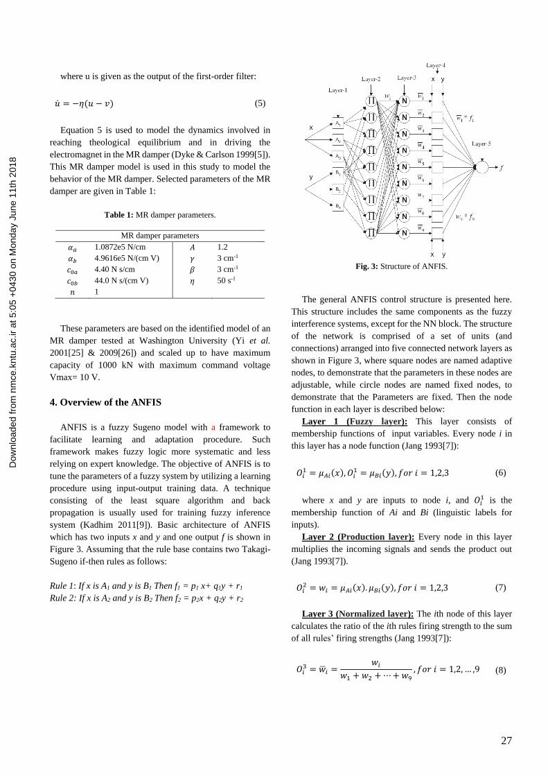
system (Kadhim 2011[9]). Basic architecture of ANFIS
which has two inputs x and y and one output f is shown in
Figure 3. Assuming that the rule base contains two Takagi-
Sugeno if-then rules as follows:
Rule 1: If x is A1 and y is B1 Then f1 = p1 x+ q1y + r1
Rule 2: If x is A2 and y is B2 Then f2 = p2x + q2y + r2
Fig. 3: Structure of ANFIS.
The general ANFIS control structure is presented here.
This structure includes the same components as the fuzzy
interference systems, except for the NN block. The structure
of the network is comprised of a set of units (and
connections) arranged into five connected network layers as
shown in Figure 3, where square nodes are named adaptive
nodes, to demonstrate that the parameters in these nodes are
adjustable, while circle nodes are named fixed nodes, to
demonstrate that the Parameters are fixed. Then the node
function in each layer is described below:
Layer 1 (Fuzzy layer): This layer consists of
membership functions of input variables. Every node i in
this layer has a node function (Jang 1993[7]):
𝑂𝑖1 = 𝜇𝐴𝑖(𝑥), 𝑂𝑖
1 = 𝜇𝐵𝑖(𝑦), 𝑓𝑜𝑟 𝑖 = 1,2,3 (6)
where x and y are inputs to node i, and 𝑂𝑖1 is the
membership function of Ai and Bi (linguistic labels for
inputs).
Layer 2 (Production layer): Every node in this layer
multiplies the incoming signals and sends the product out
(Jang 1993[7]).
𝑂𝑖2 = 𝑤𝑖 = 𝜇𝐴𝑖(𝑥). 𝜇𝐵𝑖(𝑦), 𝑓𝑜𝑟 𝑖 = 1,2,3 (7)
Layer 3 (Normalized layer): The ith node of this layer
calculates the ratio of the ith rules firing strength to the sum
of all rules’ firing strengths (Jang 1993[7]):
𝑂𝑖3 = �̅�𝑖 =
𝑤𝑖
𝑤1 + 𝑤2 + ⋯ + 𝑤9, 𝑓𝑜𝑟 𝑖 = 1,2, … ,9 (8)
Dow
nloa
ded
from
nm
ce.k
ntu.
ac.ir
at 5
:05
+04
30 o
n M
onda
y Ju
ne 1
1th
2018
Numerical Methods in Civil Engineering, Vol. 2, No. 1, September. 2017
Layer 4 (Defuzzy layer): Every node i in this layer has a
node function (Jang 1993[7]):
𝑂𝑖4 = �̅�𝑖 . 𝑓𝑖 = �̅�𝑖 . (𝑝𝑖𝑥 + 𝑞𝑖𝑦 + 𝑟𝑖) (9)
where wi is the output of layer 3 and {pi, qi, ri} is the
parameter set. Parameters in this layer will be referred to as
consequent parameters.
Layer 5 (overall output layer): This layer sums up all
the inputs coming from layer 4 and transforms the fuzzy
classification results into a crisp (Jang 1993[7]).
𝑂𝑖5 = ∑ �̅�𝑖𝑓𝑖
𝑖
=∑ 𝑤𝑖𝑓𝑖𝑖
∑ 𝑤𝑖𝑖
(10)
The ANFIS structure is adjusted automatically by least-
square estimation & the back propagation algorithm.
Because of its flexibility, the ANFIS strategy can be used for
a wide range of control applications (Kusagur et al.
2010[13]).
5. ANFIS Inverse Training
The structure of the ANFIS inverse based control system
is mainly composed of the ANFIS inverse network of the
plant, which is used as a controller to generate the control
action. To obtain the ANFIS inverse model of a plant, it is
placed in series with the plant as shown in Figure 4. For the
training, the input-output data set is used to reflect input-
output characteristics of the plant.
Fig. 4: The training process of ANFIS based on inverse plant
model.
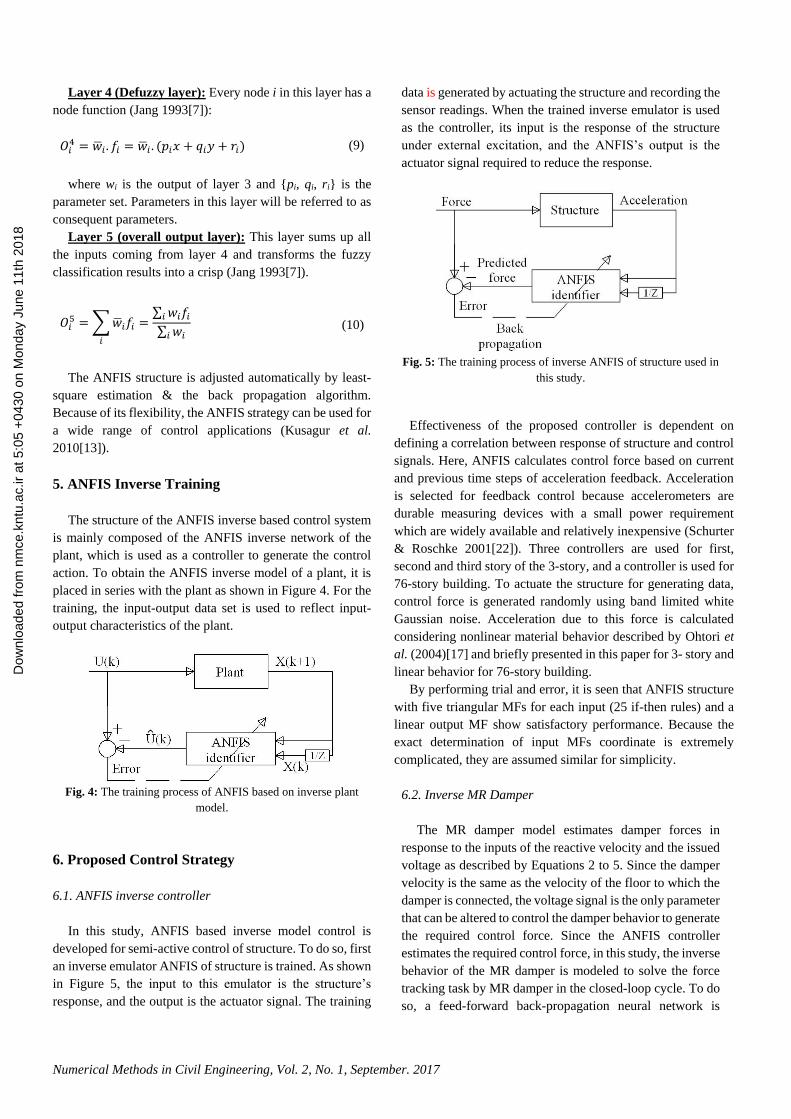
6. Proposed Control Strategy
6.1. ANFIS inverse controller
In this study, ANFIS based inverse model control is
developed for semi-active control of structure. To do so, first
an inverse emulator ANFIS of structure is trained. As shown
in Figure 5, the input to this emulator is the structure’s
response, and the output is the actuator signal. The training
data is generated by actuating the structure and recording the
sensor readings. When the trained inverse emulator is used
as the controller, its input is the response of the structure
under external excitation, and the ANFIS’s output is the
actuator signal required to reduce the response.
Fig. 5: The training process of inverse ANFIS of structure used in
this study.
Effectiveness of the proposed controller is dependent on
defining a correlation between response of structure and control
signals. Here, ANFIS calculates control force based on current
and previous time steps of acceleration feedback. Acceleration
is selected for feedback control because accelerometers are
durable measuring devices with a small power requirement
which are widely available and relatively inexpensive (Schurter
& Roschke 2001[22]). Three controllers are used for first,
second and third story of the 3-story, and a controller is used for
76-story building. To actuate the structure for generating data,
control force is generated randomly using band limited white
Gaussian noise. Acceleration due to this force is calculated
considering nonlinear material behavior described by Ohtori et
al. (2004)[17] and briefly presented in this paper for 3- story and
linear behavior for 76-story building.
By performing trial and error, it is seen that ANFIS structure
with five triangular MFs for each input (25 if-then rules) and a
linear output MF show satisfactory performance. Because the
exact determination of input MFs coordinate is extremely
complicated, they are assumed similar for simplicity.
6.2. Inverse MR Damper
The MR damper model estimates damper forces in
response to the inputs of the reactive velocity and the issued
voltage as described by Equations 2 to 5. Since the damper
velocity is the same as the velocity of the floor to which the
damper is connected, the voltage signal is the only parameter
that can be altered to control the damper behavior to generate
the required control force. Since the ANFIS controller
estimates the required control force, in this study, the inverse
behavior of the MR damper is modeled to solve the force
tracking task by MR damper in the closed-loop cycle. To do
so, a feed-forward back-propagation neural network is
Dow
nloa
ded
from
nm
ce.k
ntu.
ac.ir
at 5
:05
+04
30 o
n M
onda
y Ju
ne 1
1th
2018
29
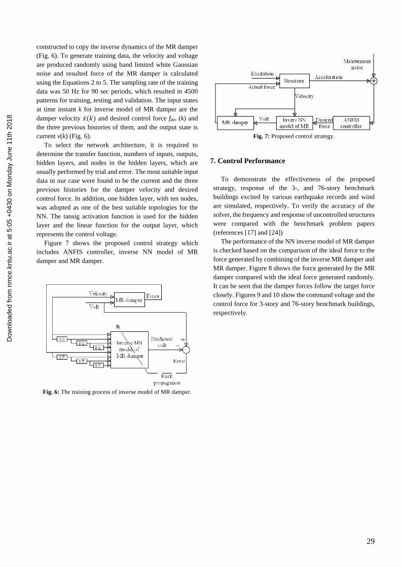
constructed to copy the inverse dynamics of the MR damper
(Fig. 6). To generate training data, the velocity and voltage
are produced randomly using band limited white Gaussian
noise and resulted force of the MR damper is calculated
using the Equations 2 to 5. The sampling rate of the training
data was 50 Hz for 90 sec periods, which resulted in 4500
patterns for training, testing and validation. The input states
at time instant k for inverse model of MR damper are the
damper velocity �̇�(𝑘) and desired control force fdes (k) and
the three previous histories of them, and the output state is
current v(k) (Fig. 6).
To select the network architecture, it is required to
determine the transfer function, numbers of inputs, outputs,
hidden layers, and nodes in the hidden layers, which are
usually performed by trial and error. The most suitable input
data in our case were found to be the current and the three
previous histories for the damper velocity and desired
control force. In addition, one hidden layer, with ten nodes,
was adopted as one of the best suitable topologies for the
NN. The tansig activation function is used for the hidden
layer and the linear function for the output layer, which
represents the control voltage.
Figure 7 shows the proposed control strategy which
includes ANFIS controller, inverse NN model of MR
damper and MR damper.
Fig. 6: The training process of inverse model of MR damper.
Fig. 7: Proposed control strategy.
7. Control Performance
To demonstrate the effectiveness of the proposed
strategy, response of the 3-, and 76-story benchmark
buildings excited by various earthquake records and wind
are simulated, respectively. To verify the accuracy of the
solver, the frequency and response of uncontrolled structures
were compared with the benchmark problem papers
(references [17] and [24])
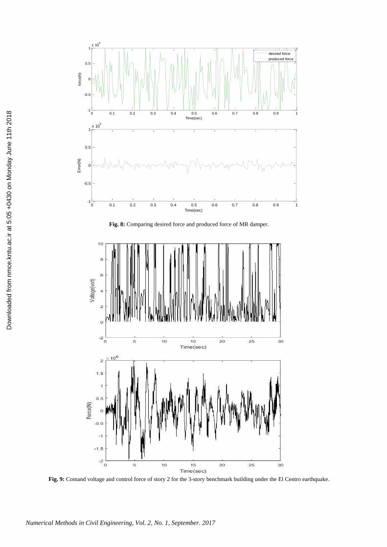
The performance of the NN inverse model of MR damper
is checked based on the comparison of the ideal force to the
force generated by combining of the inverse MR damper and
MR damper. Figure 8 shows the force generated by the MR
damper compared with the ideal force generated randomly.
It can be seen that the damper forces follow the target force
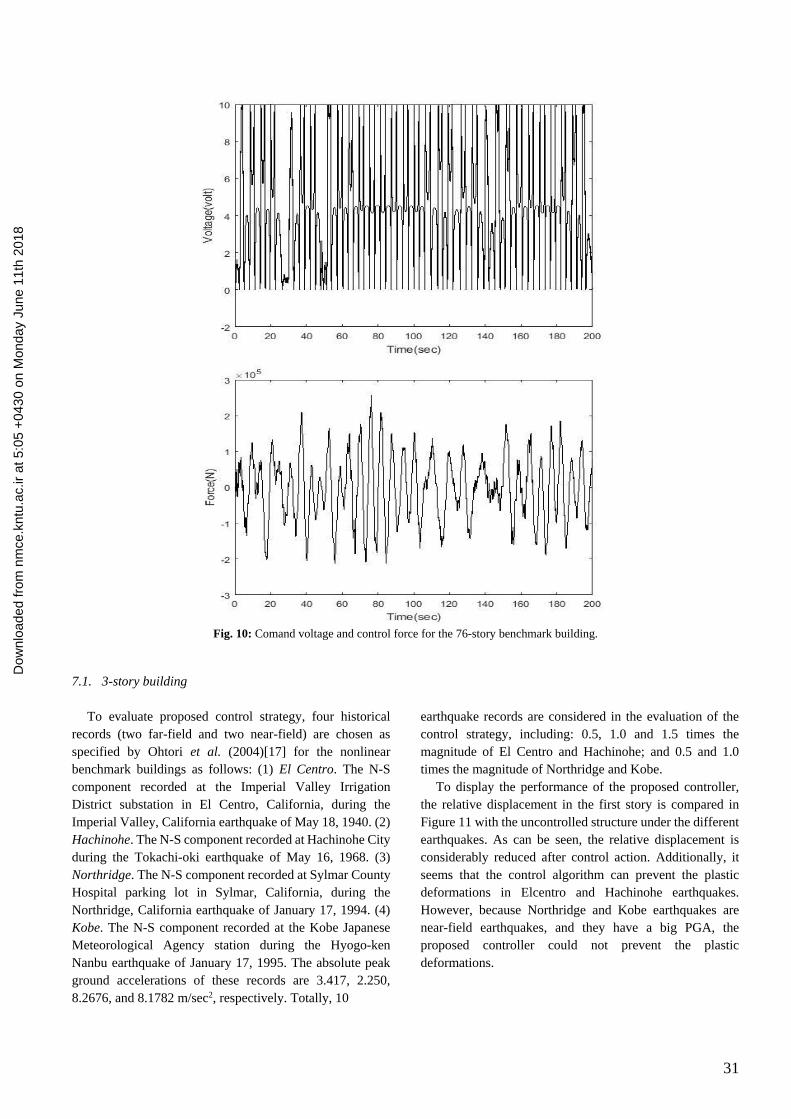
closely. Figures 9 and 10 show the command voltage and the
control force for 3-story and 76-story benchmark buildings,
respectively.
Dow
nloa
ded
from
nm
ce.k
ntu.
ac.ir
at 5
:05
+04
30 o
n M
onda
y Ju
ne 1
1th
2018
Numerical Methods in Civil Engineering, Vol. 2, No. 1, September. 2017
Fig. 8: Comparing desired force and produced force of MR damper.
Fig. 9: Comand voltage and control force of story 2 for the 3-story benchmark building under the El Centro earthquake.
0 0.1 0.2 0.3 0.4 0.5 0.6 0.7 0.8 0.9 1-1
-0.5
0
0.5
1x 10
6
Time(sec)
forc
e(N
)
desired force
produced force
0 0.1 0.2 0.3 0.4 0.5 0.6 0.7 0.8 0.9 1-1
-0.5
0
0.5
1x 10
6
Time(sec)
Err
or(
N)
Dow
nloa
ded
from
nm
ce.k
ntu.
ac.ir
at 5
:05
+04
30 o
n M
onda
y Ju
ne 1
1th
2018
31
Fig. 10: Comand voltage and control force for the 76-story benchmark building.
7.1. 3-story building
To evaluate proposed control strategy, four historical
records (two far-field and two near-field) are chosen as
specified by Ohtori et al. (2004)[17] for the nonlinear
benchmark buildings as follows: (1) El Centro. The N-S
component recorded at the Imperial Valley Irrigation
District substation in El Centro, California, during the
Imperial Valley, California earthquake of May 18, 1940. (2)
Hachinohe. The N-S component recorded at Hachinohe City
during the Tokachi-oki earthquake of May 16, 1968. (3)
Northridge. The N-S component recorded at Sylmar County
Hospital parking lot in Sylmar, California, during the
Northridge, California earthquake of January 17, 1994. (4)
Kobe. The N-S component recorded at the Kobe Japanese
Meteorological Agency station during the Hyogo-ken
Nanbu earthquake of January 17, 1995. The absolute peak
ground accelerations of these records are 3.417, 2.250,
8.2676, and 8.1782 m/sec2, respectively. Totally, 10
earthquake records are considered in the evaluation of the
control strategy, including: 0.5, 1.0 and 1.5 times the
magnitude of El Centro and Hachinohe; and 0.5 and 1.0
times the magnitude of Northridge and Kobe.
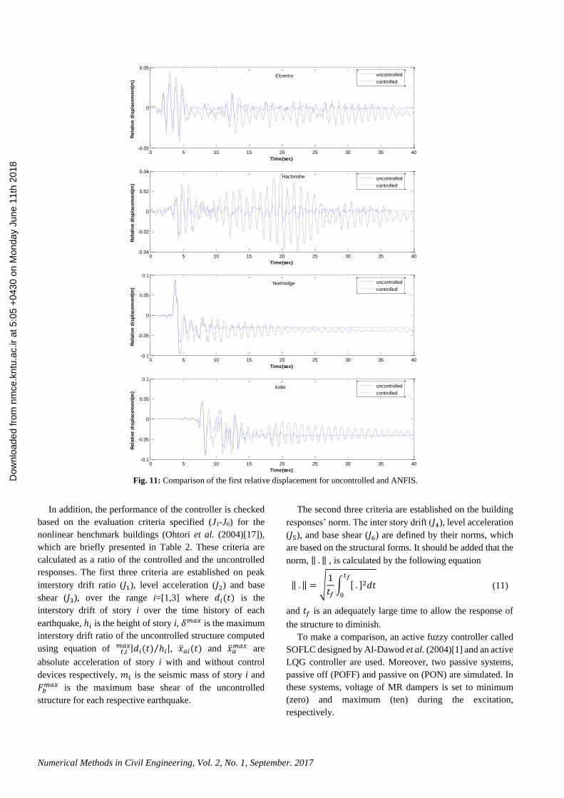
To display the performance of the proposed controller,
the relative displacement in the first story is compared in
Figure 11 with the uncontrolled structure under the different
earthquakes. As can be seen, the relative displacement is
considerably reduced after control action. Additionally, it
seems that the control algorithm can prevent the plastic
deformations in Elcentro and Hachinohe earthquakes.
However, because Northridge and Kobe earthquakes are
near-field earthquakes, and they have a big PGA, the
proposed controller could not prevent the plastic
deformations.
Dow
nloa
ded
from
nm
ce.k
ntu.
ac.ir
at 5
:05
+04
30 o
n M
onda
y Ju
ne 1
1th
2018
Numerical Methods in Civil Engineering, Vol. 2, No. 1, September. 2017
Fig. 11: Comparison of the first relative displacement for uncontrolled and ANFIS.
In addition, the performance of the controller is checked
based on the evaluation criteria specified (J1-J6) for the
nonlinear benchmark buildings (Ohtori et al. (2004)[17]),
which are briefly presented in Table 2. These criteria are
calculated as a ratio of the controlled and the uncontrolled
responses. The first three criteria are established on peak
interstory drift ratio (𝐽1), level acceleration (𝐽2) and base
shear (𝐽3), over the range i=[1,3] where 𝑑𝑖(𝑡) is the
interstory drift of story i over the time history of each
earthquake, ℎ𝑖 is the height of story i, 𝛿𝑚𝑎𝑥 is the maximum
interstory drift ratio of the uncontrolled structure computed
using equation of |𝑑𝑖(𝑡) ℎ𝑖⁄ |𝑡,𝑖 𝑚𝑎𝑥 , �̈�𝑎𝑖(𝑡) and �̈�𝑎
𝑚𝑎𝑥 are
absolute acceleration of story i with and without control
devices respectively, 𝑚𝑖 is the seismic mass of story i and
𝐹𝑏𝑚𝑎𝑥 is the maximum base shear of the uncontrolled
structure for each respective earthquake.
The second three criteria are established on the building
responses’ norm. The inter story drift (𝐽4), level acceleration
(𝐽5), and base shear (𝐽6) are defined by their norms, which
are based on the structural forms. It should be added that the
norm, ‖ . ‖ , is calculated by the following equation
‖ . ‖ = √1
𝑡𝑓∫ [ . ]2𝑑𝑡
𝑡𝑓
0
(11)
and 𝑡𝑓 is an adequately large time to allow the response of
the structure to diminish.
To make a comparison, an active fuzzy controller called
SOFLC designed by Al-Dawod et al. (2004)[1] and an active
LQG controller are used. Moreover, two passive systems,
passive off (POFF) and passive on (PON) are simulated. In
these systems, voltage of MR dampers is set to minimum
(zero) and maximum (ten) during the excitation,
respectively.
0 5 10 15 20 25 30 35 40-0.05
0
0.05
Time(sec)
Rela
tive d
isp
lacem
en
t(m
)
Elcentro uncontrolled
controlled
0 5 10 15 20 25 30 35 40-0.04
-0.02
0
0.02
0.04
Time(sec)
Rela
tive d
isp
lacem
en
t(m
)
Hachinohe uncontrolled
controlled
0 5 10 15 20 25 30 35 40-0.1
-0.05
0
0.05
0.1
Time(sec)
Rela
tive d
isp
lacem
en
t(m
)
Northridge uncontrolled
controlled
0 5 10 15 20 25 30 35 40-0.1
-0.05
0
0.05
0.1
Time(sec)
Rela
tive d
isp
lacem
en
t(m
)
kobe uncontrolled
controlled
Dow
nloa
ded
from
nm
ce.k
ntu.
ac.ir
at 5
:05
+04
30 o
n M
onda
y Ju
ne 1
1th
2018
33
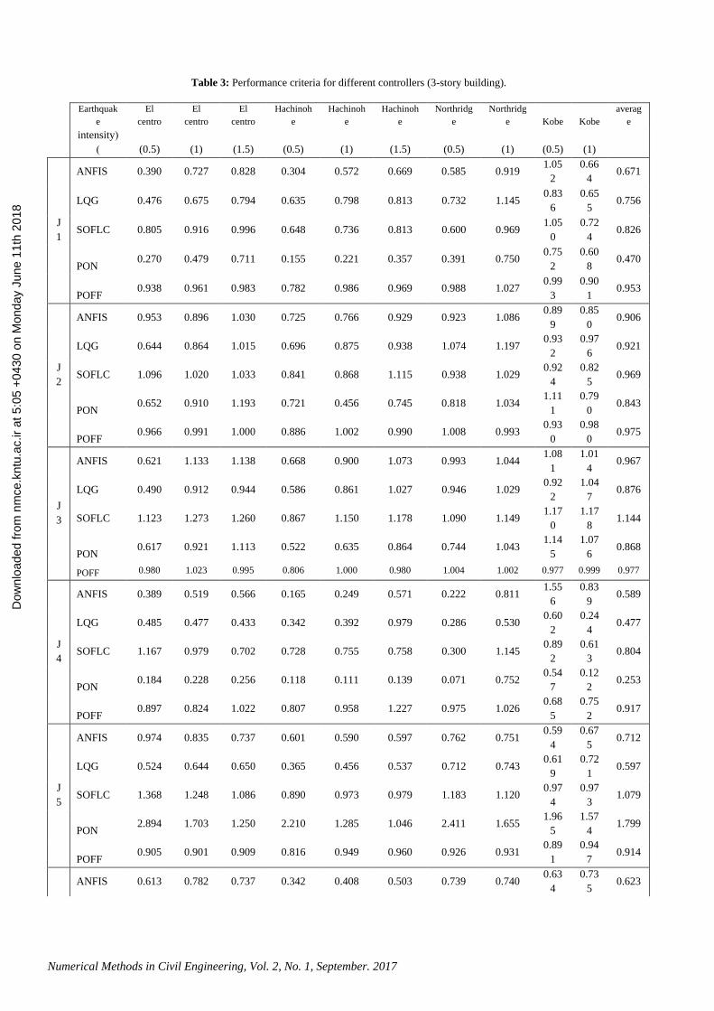
Table 3 presents the evaluation criteria as the ratio of the
controlled response to the uncontrolled response for each
earthquake record individually for proposed controller
(ANFIS), LQG, SOFLC, passive on and passive off control
systems. This table shows that the proposed control system
reduced J1, J2, J3, J4, J5 and J6, 33%, 9%, 3%, 29%, 38%,
and 41%, respectively. In other words, ANFIS has a
significant effect on normed interstory drift, acceleration and
base shear and also peak of interstory drift, but a poor effect
on peak acceleration and base shear. Comparing ANFIS and
LQG controllers shows that the LQG performed slightly
better than ANFIS controller.
Results also show that the passive on the system
performed better than other systems in most criteria,
especially the criteria associated to drift. This system
decreased J1 and J4, 53% and 75% and also decreased J2, J3
and J6, 16%, 13%, and 25%, respectively. Unfortunately, the
normed acceleration is increased 80% using passive on the
system; therefore, this system can’t be used where occupant
comfort is a high priority.
Table 3 also shows that passive off and SOFLC were by
far the worst control systems, especially SOFLC that
increased peak base shear, normed acceleration and normed
base shear, 14%, 8%, and 27%, respectively.
7.2. 76-story building
In addition to simulation of the 3-story building under
earthquake excitations, here, the 76-story benchmark
building equipped with MR and TMD dampers is simulated
under 500 seconds wind excitation to evaluate the proposed
control strategy. The wind velocity can be separated into an
average wind velocity and a wind fluctuation component.
Consequently, the wind load composed of a static load due
to the average wind velocity and a dynamic load due to wind
velocity fluctuations. For structural control, only the
fluctuating wind loads will be considered. Since the building
is symmetric in both horizontal directions, the axis of elastic
centers and the axis of mass centers coincide; therefore,
there is no coupled lateral-torsional motion. Further, to
reduce the computational efforts, only the along-wind
motion will be considered. The Davenport wind load
spectrum, which has been used in the Canadian design code,
is used herein for along-wind loads.
The performance of the controller is evaluated based on
the correlation of the response of controlled and
uncontrolled building. Moreover, active LQG controller and
passive TMD (PTMD) are used for comparison. Responses
which are checked herein are the peak and RMS of
displacement and acceleration for stories 1, 30, 50, 55, 60,
65, 70, 75 and 76.
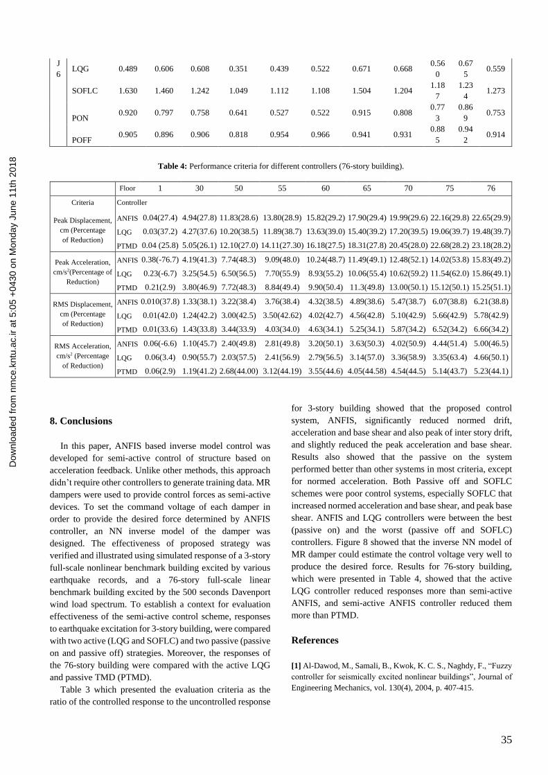
Table 4 presents the results for different controllers and
different stories. This table shows that the proposed
controller (ANFIS) reduced the peak and RMS displacement
of stories about 30% and 38%, respectively. In addition, the
peak and RMS acceleration of stories are decreased about
50%.
Comparing the result for ANFIS and PTMD shows that
although ANFIS didn’t decrease the peak acceleration as
much as PTMD, it decreased the peak and RMS
displacement and RMS acceleration more than PTMD in
deferent stories. Table 4 also shows that the active LQG
controller reduced displacement and acceleration more than
the proposed controller.
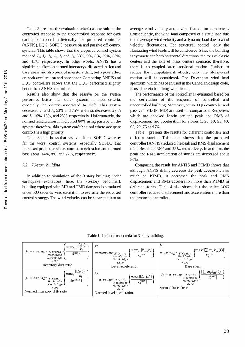
Table 2: Performance criteria for 3- story building.
𝐽1 = 𝑎𝑣𝑒𝑟𝑎𝑔𝑒 𝐸𝑙 𝐶𝑒𝑛𝑡𝑟𝑜𝐻𝑎𝑐ℎ𝑖𝑛𝑜ℎ𝑒𝑁𝑜𝑟𝑡ℎ𝑟𝑖𝑑𝑔𝑒
𝐾𝑜𝑏𝑒
{𝑚𝑎𝑥𝑡,𝑖
|𝑑𝑖(𝑡)|ℎ𝑖
𝛿𝑚𝑎𝑥}
Interstory drift ratio
𝐽2
= 𝑎𝑣𝑒𝑟𝑎𝑔𝑒 𝐸𝑙 𝐶𝑒𝑛𝑡𝑟𝑜𝐻𝑎𝑐ℎ𝑖𝑛𝑜ℎ𝑒𝑁𝑜𝑟𝑡ℎ𝑟𝑖𝑑𝑔𝑒
𝐾𝑜𝑏𝑒
{𝑚𝑎𝑥𝑡,𝑖|�̈�𝑎𝑖(𝑡)|
�̈�𝑎𝑚𝑎𝑥 }
Level acceleration
𝐽3
= 𝑎𝑣𝑒𝑟𝑎𝑔𝑒 𝐸𝑙 𝐶𝑒𝑛𝑡𝑟𝑜𝐻𝑎𝑐ℎ𝑖𝑛𝑜ℎ𝑒𝑁𝑜𝑟𝑡ℎ𝑟𝑖𝑑𝑔𝑒
𝐾𝑜𝑏𝑒
{𝑚𝑎𝑥𝑡|∑ 𝑚𝑖�̈�𝑎𝑖(𝑡)𝑖 |
𝐹𝑏𝑚𝑎𝑥 }
Base shear
𝐽4 = 𝑎𝑣𝑒𝑟𝑎𝑔𝑒 𝐸𝑙 𝐶𝑒𝑛𝑡𝑟𝑜𝐻𝑎𝑐ℎ𝑖𝑛𝑜ℎ𝑒𝑁𝑜𝑟𝑡ℎ𝑟𝑖𝑑𝑔𝑒
𝐾𝑜𝑏𝑒
{𝑚𝑎𝑥𝑖
‖𝑑𝑖(𝑡)‖ℎ𝑖
‖𝛿𝑚𝑎𝑥‖}
Normed interstory drift ratio
𝐽5
= 𝑎𝑣𝑒𝑟𝑎𝑔𝑒 𝐸𝑙 𝐶𝑒𝑛𝑡𝑟𝑜𝐻𝑎𝑐ℎ𝑖𝑛𝑜ℎ𝑒𝑁𝑜𝑟𝑡ℎ𝑟𝑖𝑑𝑔𝑒
𝐾𝑜𝑏𝑒
{𝑚𝑎𝑥𝑖‖�̈�𝑎𝑖(𝑡)‖
‖�̈�𝑎𝑚𝑎𝑥‖
}
Normed level acceleration
𝐽6 = 𝑎𝑣𝑒𝑟𝑎𝑔𝑒 𝐸𝑙 𝐶𝑒𝑛𝑡𝑟𝑜𝐻𝑎𝑐ℎ𝑖𝑛𝑜ℎ𝑒𝑁𝑜𝑟𝑡ℎ𝑟𝑖𝑑𝑔𝑒
𝐾𝑜𝑏𝑒
{‖∑ 𝑚𝑖�̈�𝑎𝑖(𝑡)𝑖 ‖
‖𝐹𝑏𝑚𝑎𝑥‖
}
Normed base shear
Dow
nloa
ded
from
nm
ce.k
ntu.
ac.ir
at 5
:05
+04
30 o
n M
onda
y Ju
ne 1
1th
2018
Numerical Methods in Civil Engineering, Vol. 2, No. 1, September. 2017
Table 3: Performance criteria for different controllers (3-story building).
Earthquak
e
El
centro
El
centro
El
centro
Hachinoh
e
Hachinoh
e
Hachinoh
e
Northridg
e
Northridg
e Kobe Kobe
averag
e
(intensity
) (0.5) (1) (1.5) (0.5) (1) (1.5) (0.5) (1) (0.5) (1)
J
1
ANFIS 0.390 0.727 0.828 0.304 0.572 0.669 0.585 0.919 1.05
2
0.66
4 0.671
LQG 0.476 0.675 0.794 0.635 0.798 0.813 0.732 1.145 0.83
6
0.65
5 0.756
SOFLC 0.805 0.916 0.996 0.648 0.736 0.813 0.600 0.969 1.05
0
0.72
4 0.826
PON 0.270 0.479 0.711 0.155 0.221 0.357 0.391 0.750
0.75
2
0.60
8 0.470
POFF 0.938 0.961 0.983 0.782 0.986 0.969 0.988 1.027
0.99
3
0.90
1 0.953
J
2
ANFIS 0.953 0.896 1.030 0.725 0.766 0.929 0.923 1.086 0.89
9
0.85
0 0.906
LQG 0.644 0.864 1.015 0.696 0.875 0.938 1.074 1.197 0.93
2
0.97
6 0.921
SOFLC 1.096 1.020 1.033 0.841 0.868 1.115 0.938 1.029 0.92
4
0.82
5 0.969
PON 0.652 0.910 1.193 0.721 0.456 0.745 0.818 1.034
1.11
1
0.79
0 0.843
POFF 0.966 0.991 1.000 0.886 1.002 0.990 1.008 0.993
0.93
0
0.98
0 0.975
J
3
ANFIS 0.621 1.133 1.138 0.668 0.900 1.073 0.993 1.044 1.08
1
1.01
4 0.967
LQG 0.490 0.912 0.944 0.586 0.861 1.027 0.946 1.029 0.92
2
1.04
7 0.876
SOFLC 1.123 1.273 1.260 0.867 1.150 1.178 1.090 1.149 1.17
0
1.17
8 1.144
PON 0.617 0.921 1.113 0.522 0.635 0.864 0.744 1.043
1.14
5
1.07
6 0.868
POFF 0.980 1.023 0.995 0.806 1.000 0.980 1.004 1.002 0.977 0.999 0.977
J
4
ANFIS 0.389 0.519 0.566 0.165 0.249 0.571 0.222 0.811 1.55
6
0.83
9 0.589
LQG 0.485 0.477 0.433 0.342 0.392 0.979 0.286 0.530 0.60
2
0.24
4 0.477
SOFLC 1.167 0.979 0.702 0.728 0.755 0.758 0.300 1.145 0.89
2
0.61
3 0.804
PON 0.184 0.228 0.256 0.118 0.111 0.139 0.071 0.752
0.54
7
0.12
2 0.253
POFF 0.897 0.824 1.022 0.807 0.958 1.227 0.975 1.026
0.68
5
0.75
2 0.917
J
5
ANFIS 0.974 0.835 0.737 0.601 0.590 0.597 0.762 0.751 0.59
4
0.67
5 0.712
LQG 0.524 0.644 0.650 0.365 0.456 0.537 0.712 0.743 0.61
9
0.72
1 0.597
SOFLC 1.368 1.248 1.086 0.890 0.973 0.979 1.183 1.120 0.97
4
0.97
3 1.079
PON 2.894 1.703 1.250 2.210 1.285 1.046 2.411 1.655
1.96
5
1.57
4 1.799
POFF 0.905 0.901 0.909 0.816 0.949 0.960 0.926 0.931
0.89
1
0.94
7 0.914
ANFIS 0.613 0.782 0.737 0.342 0.408 0.503 0.739 0.740
0.63
4
0.73
5 0.623
Dow
nloa
ded
from
nm
ce.k
ntu.
ac.ir
at 5
:05
+04
30 o
n M
onda
y Ju
ne 1
1th
2018
35
J
6
LQG 0.489 0.606 0.608 0.351 0.439 0.522 0.671 0.668 0.56
0
0.67
5 0.559
SOFLC 1.630 1.460 1.242 1.049 1.112 1.108 1.504 1.204 1.18
7
1.23
4 1.273
PON 0.920 0.797 0.758 0.641 0.527 0.522 0.915 0.808
0.77
3
0.86
9 0.753
POFF 0.905 0.896 0.906 0.818 0.954 0.966 0.941 0.931
0.88
5
0.94
2 0.914
Table 4: Performance criteria for different controllers (76-story building).
Floor 1 30 50 55 60 65 70 75 76
Criteria Controller
Peak Displacement,
cm (Percentage
of Reduction)
ANFIS 0.04(27.4) 4.94(27.8) 11.83(28.6) 13.80(28.9) 15.82(29.2) 17.90(29.4) 19.99(29.6) 22.16(29.8) 22.65(29.9)
LQG 0.03(37.2) 4.27(37.6) 10.20(38.5) 11.89(38.7) 13.63(39.0) 15.40(39.2) 17.20(39.5) 19.06(39.7) 19.48(39.7)
PTMD 0.04 (25.8) 5.05(26.1) 12.10(27.0) 14.11(27.30) 16.18(27.5) 18.31(27.8) 20.45(28.0) 22.68(28.2) 23.18(28.2)
Peak Acceleration,
cm/s2(Percentage of
Reduction)
ANFIS 0.38(-76.7) 4.19(41.3) 7.74(48.3) 9.09(48.0) 10.24(48.7) 11.49(49.1) 12.48(52.1) 14.02(53.8) 15.83(49.2)
LQG 0.23(-6.7) 3.25(54.5) 6.50(56.5) 7.70(55.9) 8.93(55.2) 10.06(55.4) 10.62(59.2) 11.54(62.0) 15.86(49.1)
PTMD 0.21(2.9) 3.80(46.9) 7.72(48.3) 8.84(49.4) 9.90(50.4) 11.3(49.8) 13.00(50.1) 15.12(50.1) 15.25(51.1)
RMS Displacement,
cm (Percentage
of Reduction)
ANFIS 0.010(37.8) 1.33(38.1) 3.22(38.4) 3.76(38.4) 4.32(38.5) 4.89(38.6) 5.47(38.7) 6.07(38.8) 6.21(38.8)
LQG 0.01(42.0) 1.24(42.2) 3.00(42.5) 3.50(42.62) 4.02(42.7) 4.56(42.8) 5.10(42.9) 5.66(42.9) 5.78(42.9)
PTMD 0.01(33.6) 1.43(33.8) 3.44(33.9) 4.03(34.0) 4.63(34.1) 5.25(34.1) 5.87(34.2) 6.52(34.2) 6.66(34.2)
RMS Acceleration,
cm/s2 (Percentage
of Reduction)
ANFIS 0.06(-6.6) 1.10(45.7) 2.40(49.8) 2.81(49.8) 3.20(50.1) 3.63(50.3) 4.02(50.9) 4.44(51.4) 5.00(46.5)
LQG 0.06(3.4) 0.90(55.7) 2.03(57.5) 2.41(56.9) 2.79(56.5) 3.14(57.0) 3.36(58.9) 3.35(63.4) 4.66(50.1)
PTMD 0.06(2.9) 1.19(41.2) 2.68(44.00) 3.12(44.19) 3.55(44.6) 4.05(44.58) 4.54(44.5) 5.14(43.7) 5.23(44.1)
8. Conclusions
In this paper, ANFIS based inverse model control was
developed for semi-active control of structure based on
acceleration feedback. Unlike other methods, this approach
didn’t require other controllers to generate training data. MR
dampers were used to provide control forces as semi-active
devices. To set the command voltage of each damper in
order to provide the desired force determined by ANFIS
controller, an NN inverse model of the damper was
designed. The effectiveness of proposed strategy was
verified and illustrated using simulated response of a 3-story
full-scale nonlinear benchmark building excited by various
earthquake records, and a 76-story full-scale linear
benchmark building excited by the 500 seconds Davenport
wind load spectrum. To establish a context for evaluation
effectiveness of the semi-active control scheme, responses
to earthquake excitation for 3-story building, were compared
with two active (LQG and SOFLC) and two passive (passive
on and passive off) strategies. Moreover, the responses of
the 76-story building were compared with the active LQG
and passive TMD (PTMD).
Table 3 which presented the evaluation criteria as the
ratio of the controlled response to the uncontrolled response
for 3-story building showed that the proposed control
system, ANFIS, significantly reduced normed drift,
acceleration and base shear and also peak of inter story drift,
and slightly reduced the peak acceleration and base shear.
Results also showed that the passive on the system
performed better than other systems in most criteria, except
for normed acceleration. Both Passive off and SOFLC
schemes were poor control systems, especially SOFLC that
increased normed acceleration and base shear, and peak base
shear. ANFIS and LQG controllers were between the best
(passive on) and the worst (passive off and SOFLC)
controllers. Figure 8 showed that the inverse NN model of
MR damper could estimate the control voltage very well to
produce the desired force. Results for 76-story building,
which were presented in Table 4, showed that the active
LQG controller reduced responses more than semi-active
ANFIS, and semi-active ANFIS controller reduced them
more than PTMD.
References
[1] Al-Dawod, M., Samali, B., Kwok, K. C. S., Naghdy, F., “Fuzzy
controller for seismically excited nonlinear buildings”, Journal of
Engineering Mechanics, vol. 130(4), 2004, p. 407-415.
Dow
nloa
ded
from
nm
ce.k
ntu.
ac.ir
at 5
:05
+04
30 o
n M
onda
y Ju
ne 1
1th
2018
Numerical Methods in Civil Engineering, Vol. 2, No. 1, September. 2017
[2] Bani-Hani, K. A., Mashal, A., Sheban, M. A., “Semi-active
neuro-control for base-isolation system using magnetorheological
(MR) dampers”, Earthquake Engineering & Structural Dynamics,
vol. 35, 2006, p. 1119–1144.
[3] Choi, K. M., Cho, S. W., Jung, H. J., Lee, I. W., “Semi-active
fuzzy control for seismic response reduction using
magnetorheological dampers”, Earthquake Engng Struct. Dyn.,
vol. 33, 2004, p. 723–736.
[4] Dyke, S. J., Spencer, B. F., Sain, M. K., Carlson, J. D.,
“Modeling and control of magnetorheological dampers for seismic
response reduction”, Smart Materials and Structures, vol. 5, 1996,
p. 565–575.
[5] Dyke, S. J., Yi, F., Carlson, J. D., “Application of
magnetorheological dampers to seismically excited structures”,
Proc., Int. Modal Anal. Conf., Bethel, Conn, 1999.
[6] Gu, Z. Q., Oyadiji, S. O., “Application of MR damper in
structural control using ANFIS method”, Computers and
Structures, vol. 86, 2008, p. 427–436.
[7] Jang, J. S. R., “ANFIS: Adaptive network-based fuzzy
inference systems”, IEEE Transactions on Systems, Man, and
Cybernetics, vol. 23, 1993, p. 665–685.
[8] Jung, H. J., Lee, H. J., Yoon, W. H., Oh, J. W., Lee, I. W.,
“Semiactive neurocontrol for seismic response reduction using
smart damping strategy”, Journal of Computing in Civil
Engineering, vol. 18(3), 2004, p. 277–280.
[9] Kadhim, H. H., “Self Learning of ANFIS Inverse Control using
Iterative Learning Technique”, International Journal of Computer
Applications, vol. 21(8), 2011, p. 24-29.
[10] Karamodin, A., Irani, F., Baghban, A., “Effectiveness of a
fuzzy controller on the damage index of nonlinear benchmark
buildings”, Scientia iranica A, vol. 19(1), 2012, p. 1-10.
[11] Kerboua, M., Benguediab, M., Megnounif, A., Benrahou, K.
H., Kaoulala, F., “Semi active control of civil structures, analytical
and numerical studies”, Physics Procedia, vol. 55, 2014, p. 301-
306.
[12] Kumar, R., Singh, S. P., Chandrawat, H. N., “MIMO adaptive
vibration control of smart structures with quickly varying
parameters: Neural networks vs classical control approach”,
Journal of Sound and Vibration, vol. 307, 2007, p. 639–661.
[13] Kusagur, A., Kodad, S. F., Ram, B. V. S., “Modeling, Design
& Simulation of an Adaptive Neuro-Fuzzy Inference System
(ANFIS) for Speed Control of Induction Motor”, International
Journal of Computer Applications, vol. 6(12), 2010, p. 29-44.
[14] K-Karamodin, A., H-Kazemi, H., Akbarzadeh-T, M. R.,
“Semi-active control of structures using neuropredictive algorithm
for MR dampers”, 14th World Conference on Earthquake
Engineering, Beijing, China, 2008.
[15] Lee, H. J., Yang, Y. G., Jung, H. J., Spencer, B. F., Lee, I. W.,
“Semi-active neurocontrol of a base isolated benchmark structure”,
Structural Control and Health Monitoring, vol. 13, 2006, p. 682–
692.
[16] Marinaki, M., Marinakis, Y., Stavroulakis, G. E., “Fuzzy
control optimized by a multi-objective differential evolution
algorithm for vibration suppression of smart structures”,
Computers & Structures, vol. 147, 2015, p. 126-137.
[17] Ohtori, Y., Christenson, R. E., Spencer, Jr. B. F., Dyke, S. J.,
“Benchmark control problems for seismically excited nonlinear
buildings”, Journal of Engineering Mechanics, vol. 130(4), 2004,
p. 366–387.
[18] Ohtori, Y., Spencer, B.F. Jr., “A MATLAB-based tool for
nonlinear structural analysis”, In the proceeding of the 13th ASCE
engineering mechanics division specialty conference, Johns
Hopkins university, Baltimore, June13-16, 1999.
[19] Park, K-S., Ok, S-Y., “Modal-space reference-model-tracking
fuzzy control of earthquake excited structures”, Journal of Sound
and Vibration, vol. 334, 2015, p. 136-150.
[20] Pourzeynali, S., Lavasani, H. H., Modarayi, A. H., “Active
control of high rise building structures using fuzzy logic and
genetic Algorithms”, Engineering Structures, vol. 29, 2007, p. 346-
357.
[21] Rezaiee-Pajand, M., Akbarzadeh-T., M. R., Nikdel, A.,
“Direct adaptive neurocontrol of structures under earth vibration”,
Journal of Computing in Civil Engineering, vol. 23(5), 2009, p.
299-307.
[22] Schurter, K. C., Roschke, P. N., “Neuro-Fuzzy Control of
Structures Using Magnetorheological Dampers”, Proceedings of
the American Control Conference, Arlington, 2001, p. 25-27.
[23] Xu, Y. L., Qu, W. L., Ko, J. M., “Seismic response control of
frame structures using magnetorheological/ electrorheological
dampers”, Earthq. Eng. Struct. Dyn., vol. 29, 2000, p. 557–75.
[24] Yang, J., Wu, J., Samali, B., Agrawal, A., “A benchmark
problem for response control of wind-excited tall building”, Web
Site (http://www.eng.uci.edu/~jnyang/benchmark.htm), 1999.
[25] Yi, F., Dyke, S. J., Caicedo, J. M., Carlson J. D.,
“Experimental Verification of Multi-Input Seismic Control
Strategies for Smart Dampers”, Journal of Engineering Mechanics,
vol. 127(11), 2001, p. 1152–1164.
[26] Yi, F., Dyke, S. J., Caicedo, J. M., Carlson, J. D., “Seismic
Response Control Using Smart Dampers”, Proc., American
Control Conference, San Diego, CA, 2009, p. 1022–1026.
Dow
nloa
ded
from
nm
ce.k
ntu.
ac.ir
at 5
:05
+04
30 o
n M
onda
y Ju
ne 1
1th
2018
Top Related