


Languages
Pages
Legal


Computing the Density of States of Boolean FormulasStefano Ermon,
Carla Gomes, and Bart Selman
Cornell University, September 2010

From 100 variables, 200 constraints (early 90’s)to over 1,000,000 vars. and 5,000,000 clausesin 20 years.
Applications: Hardware and Software Verification, Planning, Scheduling, Optimal Control, Protocol Design, Routing, Multi-agent systems, E-Commerce (E-auctions and electronic trading agents), etc.
Motivation:Significant progress in SAT
SAT: Given a Boolean formula Φ in CNF, Φ=C1ΛC2 Λ…ΛCmdoes Φ have a satisfying assignment?

Extending SAT technology Model counting problem (number of distinct
satisfying assignments): probabilistic inference problems multi-agent / adversarial reasoning (bounded)
[Roth ‘96, Littman et. al. ‘01, Sang et. al. ‘04, Darwiche ‘05,
Domingos ‘06]
MAX-SAT and Weighted MAX-SAT: find a truth assignment that maximizes the number of satisfied clauses or the sum of their weights
beyond decision (NP) [Hansen at al. ’90] hard and soft constraints [Heras et al. ’08, Cohen et al. ’06]
How can we combine both challenges?

Density of states Given a Boolean formula Φ in CNF,
Φ=C1ΛC2 Λ…ΛCm with m clauses
the density of states is a function
that gives the number of truth assignments that violate exactly i clauses, for i =0,..,m
n(0) = number of assignments that violate 0 clauses (models) n(1) = number of assignments that violate exactly 1 clause
],..,0[: mn

Density of states: a challenging problem Generalizes SAT
Decision problem: Φ is satisfiable if and only if n(0)>0
Generalizes MAX-SAT MAX-SAT is the minimum i such that n(i)>0
Generalizes #SAT Number of models = n(0)

Statistical physics
More generally, the density of states (DOS) gives the number of microstates with energy E Microstates = truth assignments Energy = number of violated clauses Ground states = maximally satisfying assignments
Compact, very informative characterization of a physical system Macroscopic thermodynamic quantities (free energy,
internal energy,..) Partition function, phase transitions,..

Motivation
DOS provides a finer characterization of the structure of a combinatorial search space
Statistical physics and CSPs: Insights on problem structure, hardness, new
algorithms, Survey Propagation [Montanari et. al. ‘07, Monasson et. al. ‘96, Mézard ’02, Parisi ‘02]
By defining different energy functions, it can be naturally used for probabilistic style inference (e.g. Markov Logic, [Domingos ‘06] )

Talk Outline
Prior work A novel sampling strategy: MCMC-FlatSat Empirical Validation
Small formulas with ground truth Synthetic formulas Random 3-SAT Large structured instances Model counting
Conclusions

Density of states: prior work
Exact Method: Enumeration (exponential) Approximate
Uniform Sampling [Belaidouni et. al. ‘02] Sample density from K random truth assignments Impractical, unlikely to hit rare assignments (e.g. solutions)
Metropolis Sampling [Rose et. al. ‘96] In theory, the density can be extracted from the Boltzmann
distribution Impractical, difficult choice of the temperature and slow
mixing times [Wei et. al. ‘04 ]
How can we improve the sampling strategy?

The flat histogram idea
Idea: Set up a Markov Chain that visits all energy levels equally often [F. Wang and Landau ’02, J. Wang
et. al. ’99, De Oliveira et. al. ’96] e.g. an equal amount of time at the set of truth assignments with 0 unsat clauses, 1 unsat clause, ...
How? Flip a variable, accept new state σ’ with probability
Always accepts “rarer” states (when n(E’)<n(E))
)(
)(,1minEn
Enp

Example
1
11
11
RED ↔ 0 unsat clauses, n(0)=1GREEN ↔ 1 unsat clauses, n(1)=3BLUE ↔ 2 unsat clauses, n(2)=10
Goal: visit all energy levels (colors) equally often

Example
3/103/10
3/10
3/10
RED ↔ 0 unsat clauses, n(0)=1GREEN ↔ 1 unsat clauses, n(1)=3BLUE ↔ 2 unsat clauses, n(2)=10
Goal: visit all energy levels (colors) equally often

Example
3/103/10
3/10
3/10
RED ↔ 0 unsat clauses, n(0)=1GREEN ↔ 1 unsat clauses, n(1)=3BLUE ↔ 2 unsat clauses, n(2)=10
Goal: visit all energy levels (colors) equally often

Example
1
11
RED ↔ 0 unsat clauses, n(0)=1GREEN ↔ 1 unsat clauses, n(1)=3BLUE ↔ 2 unsat clauses, n(2)=10
Goal: visit all energy levels (colors) equally often

Example
1
1 1
11
RED ↔ 0 unsat clauses, n(0)=1GREEN ↔ 1 unsat clauses, n(1)=3BLUE ↔ 2 unsat clauses, n(2)=10
Goal: visit all energy levels (colors) equally often

Example
1
11
11
RED ↔ 0 unsat clauses, n(0)=1GREEN ↔ 1 unsat clauses, n(1)=3BLUE ↔ 2 unsat clauses, n(2)=10
Goal: visit all energy levels (colors) equally often

Example
1
1
1
1
1
RED ↔ 0 unsat clauses, n(0)=1GREEN ↔ 1 unsat clauses, n(1)=3BLUE ↔ 2 unsat clauses, n(2)=10
Goal: visit all energy levels (colors) equally often

Example
1/10
1
1/3
1/10
1/10
RED ↔ 0 unsat clauses, n(0)=1GREEN ↔ 1 unsat clauses, n(1)=3BLUE ↔ 2 unsat clauses, n(2)=10
Goal: visit all energy levels (colors) equally often

Example
1/10
1
1/3
1/10
1/10
RED ↔ 0 unsat clauses, n(0)=1GREEN ↔ 1 unsat clauses, n(1)=3BLUE ↔ 2 unsat clauses, n(2)=10
Goal: visit all energy levels (colors) equally often

Example
…and finally…

Example RED ↔ 0 unsat clauses, n(0)=1GREEN ↔ 1 unsat clauses, n(1)=3BLUE ↔ 2 unsat clauses, n(2)=10

Flat histogram: Intuition Detailed balance holds with those
transition probabilities
Properly biased towards “rare” states But there are few “rare” states
The total time spent in each type of state is the same (flat visit histogram).
)(
)(,1minEn
Enp
(Red, Blue, Green)
Note: in contrast, Simulated Annealing concentrates sampling around low energy states (more greedy!)

Flat histogram
But… how can we even run the Markov Chain?
Acceptance probability:
The density n() is unknown and is precisely what we want to compute!
)(
)(,1minEn
Enp

Adaptive sampling
Start with an initial guess g (our estimate of the true density n)
Random walk: Use g for guidance (acceptance probability) Chain will initially not sample uniformly across energy
levels Each step, adjust g using a modification factor F Keep track of the visit histogram H
When we see a flat H, we must have the right density!

The modification factor, F
F controls the tradeoff between convergence rate and accuracy
Use large modification factors F at the beginning to get rough estimates fast convergence
Keep reducing F to get finer estimates Analogous to an annealing process

MCMC-FlatSat
Inner Loop
Initialization
Inner Loop : adaptive sampling until the visit histogram is flat (g becomes our new guess for n)
H
96 99105
0
50
100
0 (R ed) 1(G reen)
2 (B lue)

MCMC-FlatSat
OuterLoop
Reduce modification factor and repeat inner loop until g≈n

Outline of empirical validation
Empirical validation on combinatorial problems Convergence Efficiency (number of samples vs search space size) Accuracy
We study: Small formulas with ground truth Large synthetic formulas Random 3-SAT Large structured instances Model counting

Formulas with known ground truth
Instances from MAXSAT2007 competition (Ramsey, Spin Glass, Max Clique)
Direct enumeration is possible (n<=28), so we can compare our estimate with ground truth
Metrics: KL divergence:
Relative error per point
EKL Eg
En
Z
EngnD
)(
)(log)(
)||(

Spin glass instance, 27 variables, 162 clauses Needs ~ 8 *106 flips << search space size
(227≈1.3 *108)
Energy (# unsat clauses)
Log-
dens
ity
Rel
. err
or (
%)
Energy
3.1 % maximum relative error
n – ground truthg – estimateX

Instance variables clausesKL-
divergence Max rel. error Entropy
ramk3n7.ra0 21 70 3.9 E-05 2.39 % 2.45
ramk3n8.ra0 28 126 1.1 E-05 5.1 % 3.93
johnson8-2-4.clq 28 420 4.5 E-05 5.5 % 2.90
T3pm3-5555.spn 27 162 1.3 E-05 3.15 % 3.34
Ramsey Max Clique
Energy (# unsat clauses)
Log-
dens
ity
Energy (# unsat clauses)
Log-
dens
ity
n – ground truthg – estimateX
ng X

Synthetic formulas
Ground truth for larger formulas? Construct synthetic formulas
Formulas for which we derive a closed form solution for the density
Result on the composition (logical conjunction) of independent formulas (do not share variables)
The density of F is the convolution of the density of Φ with itself l times
)(...)()(),...,,( 2121 ll xxxxxxF

Instance variables clauses KL-divergence Max relative error (%) Entropy
UnifConv50_100 50 100 1.19 E-05 3.05 % 7.3
PigHoleConv410 200 750 1.26 E-07 2.2 % 33.7
Convolution of uniform densities
Convolution of pigeon hole formulas
Energy (# unsat clauses)
Log-
dens
ity
Energy (# unsat clauses)
Log-
dens
ity
Needs ~ 2*107 flips << state space size (250≈1015)
n – ground truthg – estimateX
ng X

Random k-SAT formulas
Well known phase transitions for the satisfiability property in terms of the ratio α (Φ is satisfiable ↔ nΦ(0)>0 )
Analytic result on the average density
given a truth assignment, the probability of having a clause that is violated is 1/2k for random k-SAT
nim
k
i
ki
minE 2
2
11
2
1)]([
]0)0([ nP

n=50 variables (average over 1000 instances) Needs ~ 108 flips << state space size (250≈1015)
Average DensitiesLo
g-de
nsity
Ratio clauses to var. α

Large structured instances
No ground truth known Consistency checks
Number of models, when exact model counting is feasible (# models=n(0))
Method of the moments: Sample K assignments at random, compute their
energies (unsat clauses) Compute sample moments (e.g. average energy,
2nd order moment of energy, ..) Compare with moments obtained using the
estimated density g

Large structured instances
Instance variables clauses g(0) # models Ms(1) M(1) Ms(2) M(2)
brock400 2.clq 40 1188 0 0 297.0 297.0 88365.9 88372.3
Spinglass5.pm 125 750 0 0 187.4 187.4 35249.2 35247.1
MANN a27.clq 42 1690 0 0 422.4 422.4 178709 178703
bw large.a 459 4675 1 1 995.2 995.3 996349 996634

Logistic instance Planning problem:
n=459 variables m=4675 clauses
Huge search space (2459 truth assignments), but MCMC-FlatSat returns within hours
Remarkable precision: Finds the only existing model g(0)=n(0)=1! The mode of the estimated distribution is e300 times larger than the number of
models g(0) counts the needles and the haystack!
(the moments method indicates g is accurate)
Energy (# unsat clauses)
Log-
dens
ity

Model counting Comparison with state-of-the-art model counters
SampleCount [Gomes et. al. ‘06] SampleMiniSAT [Gogate et. al. ‘07]
MCMCFlatSat is very accurate Timings are competitive when ratio clauses to variables is
not too large DOS provides guidance Information on what is not a model Overhead because it provides more information

Model counting comparison
Instance variables clausesExact # models
SampleCount SampleMiniSAT MCMC-FlatSat
Models Time
(s) Models Time
(s) Models Time
(s)
2bitmax 252 766 2.10×1029 >2.40×1028 29 2.08×1029 345 1.96×1029 1863
wff-3-3.5 150 525 1.40×10¹⁴ >1.60×10¹³ 145 1.60×10¹³ 240 1.34×10¹⁴ 393
wff-3.1.5 100 150 1.80×10²¹ >1.00×10²⁰ 240 1.58×10²¹ 128 1.83×10²¹ 21
wff-4-5.0 100 500 >8.00×10¹⁵ 120 1.09×10¹⁷ 191 8.64×10¹⁶ 189
ls8-norm 301 1603 5.40×10¹¹ >3.10×10¹⁰ 1140 2.22×10¹¹ 168 5.93×10¹¹ 2693

Conclusions Computing the density of states is a hard problem
(encompasses SAT, MAX-SAT, #SAT) MCMCFlatSat: sampling strategy adapted from physics for
combinatorial spaces that adaptively explores the space while collecting statistics Extremely accurate, very efficient (few samples) Provides a compact, rich description of the search space. New
insights about structure and local search Very general method: any property can be used for search
space partitioning. Many applications to counting and inference problems

Extra slides

Future work
SAT-specific improvements Energy saturation Energy barriers (and related normalization issues) Walksat heuristics (with Metropolis-Hastings updates)
Direct application to inference in Markov Logic Formal proof of convergence / counterexamples Application to other counting problems in
combinatorial spaces

Runtime for random 3-SAT
Search space 2^50 Flips 10^8 ≈ 2^26

Related work on random 3-SAT
Lots of work on the i=0 (i.e. SAT/UNSAT) case [Gent et. al. ‘94]
Previous experimental work for i>0 [Zhang ‘01] Different definition: “no more than i unsat clauses”
versus “exactly i unsat clauses” Location on the phase transitions Apparently, same location
Analytic results [Achlioptas et al. ‘05] We can see two phase transitions: assignments
are unlikely to violate a large number of clauses

Other phase transition
50 variables, 1000 instances

Other structured instances

Histogram flatness (formal)
Flatness condition of the visit histogram H is a necessary condition for convergence If g is equal to the true density n, the detailed balance
is satisfied by
upon convergence, the steady state probability is proportional to the reciprocal of the density of the corresponding energy level
pppp )()(
))((
1)(
Enp

Histogram flatness (formal)
Flatness condition of the visit histogram H is a necessary condition for convergence
If g=n, the visit histogram H will be flati.e. energy levels visited equally often
Problem: the density n() is unknown and is precisely what we want to compute!
cEn
cpEH
EEEE
)(|)(| )(
)()(
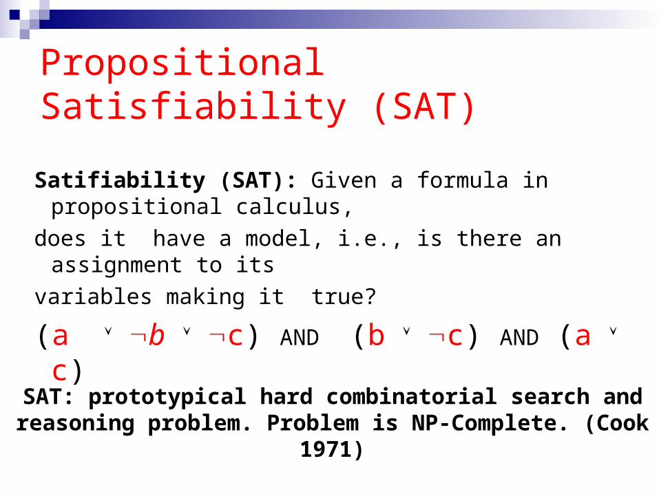
Satifiability (SAT): Given a formula in propositional calculus,
does it have a model, i.e., is there an assignment to its
variables making it true?
(a b c) AND (b c) AND (a c)
SAT: prototypical hard combinatorial search and reasoning problem. Problem is NP-Complete. (Cook 1971)
Propositional Satisfiability (SAT)

Prior work - Metropolis
Approximate [Rose et. al., ‘96 ] Metropolis sampling at temperature T Energy = number of violated clauses Measure the empirical probability P(E) of energy
levels, rescale to get the density n(E)
Slow mixing times [Wei et. al., ‘04 ] Difficult choice of the temperature
)exp()()( TEEnEP

Theoretical Convergence
Stated as a conjecture in Lee,Okabe and Landau, Convergence and
Refinement of the Wang-Landau Algorithm, Computer Physics Communications, 2006
Proof of convergence inAtchade and Liu,The Wang-Landau Algorithm for Monte Carlo computation in general state spaces, Statistica Sinica, 2009

Closed forms
k-SAT, m clauses such that each variable appears exactly in one clause, the DOS is
where is the fraction of assignments of the variables in a single clause not satisfying it (e.g. in 3-SAT, only 1 over 8 assignments does not satisfy a clause)
nEm
k
E
kE
mEn 2
2
11
2
1)(
k21

Implementation details
Use of log-densities New assignment generated by flipping a variable
uniformly at random Flatness condition (within 10% of the max) Normalization
The density is obtained only up to a constant factor We use the normalization constraint
F0=1.5, reduce by Flatness is checked every 1000 moves
E
nEg 2)(
FF

Random k-SAT formulas
k-SAT: each clause has at most k literals Random k-SAT: formulas Φ generated with
n variables m clauses produced independently by
randomly choosing a set of k variables from n available negating each one with probability 0.5
α is the ratio clauses to variables (m/n)
Let be the probability measure associated with this generative model for Φ
()P

Composition
Logical conjunction of formulas Φ that do not share variables
The density of F is the convolution of the density of Φ with itself l times
Analogous to the probability density of the sum of l independent random variables
)(...)()(),...,,( 2121 ll xxxxxxF

Closed forms
Starting with a formula Φ with uniform density (e.g. )
we construct
Sum of n s-sided dices has closed form probability distribution:
)()(),( 21212121 xxxxxxxx
),(...),(),(),...,,( 1212121 lll xxxxxxxxxF
Top Related