


Languages
Pages
Legal


ComputerVision
Non-linear tracking
Marc PollefeysCOMP 256
Some slides and illustrations from D. Forsyth, M. Isard, T. Darrell …

ComputerVision
2
Jan 16/18 - Introduction
Jan 23/25 Cameras Radiometry
Jan 30/Feb1 Sources & Shadows Color
Feb 6/8 Linear filters & edges Texture
Feb 13/15 Multi-View Geometry Stereo
Feb 20/22 Optical flow Project proposals
Feb27/Mar1 Affine SfM Projective SfM
Mar 6/8 Camera Calibration Segmentation
Mar 13/15 Springbreak Springbreak
Mar 20/22 Fitting Prob. Segmentation
Mar 27/29 Silhouettes and Photoconsistency
Linear tracking
Apr 3/5 Project Update Non-linear Tracking
Apr 10/12 Object Recognition Object Recognition
Apr 17/19 Range data Range data
Apr 24/26 Final project Final project
Tentative class schedule

ComputerVision
3
Final project presentation
No further assignments, focus on project
Final presentation: • Presentation and/or Demo
(your choice, but let me know)
• Short paper (Due April 22 by 23:59)(preferably Latex IEEE proc. style)
• Final presentation/demoApril 24 and 26
ComputerVision
4
Bayes Filters
1( , )
( , )t t t t
t t t t
x f x w
z g x v
System state dynamics
Observation dynamics
1( ) ( | , , )t t tBel x p x z z
We are interested in: Belief or posterior density
Estimating system state from noisy observations
ComputerVision
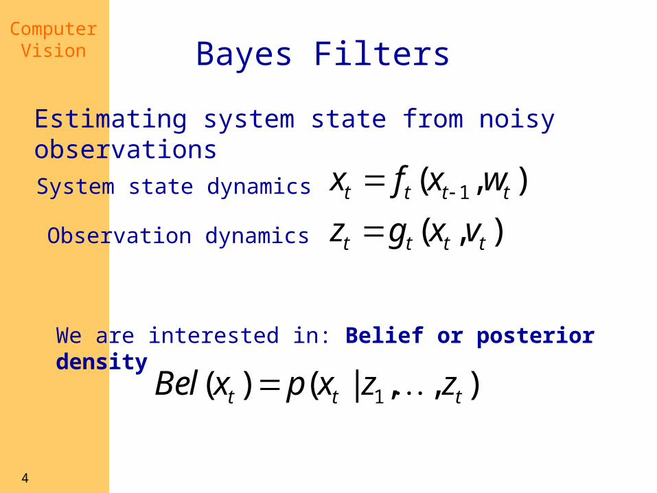
51:( 1) 1 1where , ,t tz z z
1:( 1) 1, 1:( 1) 1 1:( 1) 1( | ) ( | ) ( | )t t t t t t t tp x z p x x z p x z dx
From above, constructing two steps of Bayes Filters
1:( 1)1:( 1) 1:( 1)
1:( 1)
( | , )( | , ) ( | )
( | )t t t
t t t t tt t
p z x zp x z z p x z
p z z
Predict:
Update:
1 1 1( ) ( | ) ( )t t t t tp x p x x p x dx ( | ) ( )
( | )( )
t t tt t
t
p z x p xp x z
p z
Recall “law of total probability” and “Bayes’ rule”

ComputerVision
6
1:( 1) 1, 1:( 1) 1 1:( 1) 1( | ) ( | ) ( | )t t t t t t t tp x z p x x z p x z dx
1:( 1)replace ( | , ) with ( | )t t t t tp z x z p z x
Predict:
Update:
Assumptions: Markov Process
1 1: 1 1replace ( | , ) with ( | )t t t t tp x x z p x x
1:( 1)1:( 1) 1:( 1)
1:( 1)
( | , )( | , ) ( | )
( | )t t t
t t t t tt t
p z x zp x z z p x z
p z z
ComputerVision
7
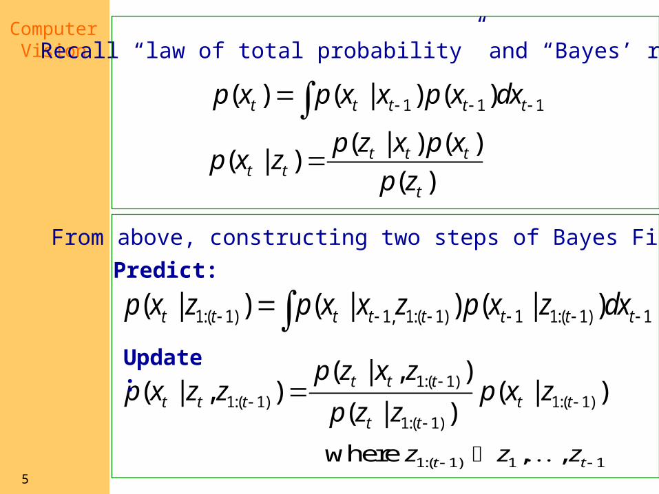
1:( 1) 1:( 1)( | , ) ( | ) ( | )t t t t t t t tp x z z p z x p x z
Bayes Filter
1:( 1) 1 1 1:( 1) 1( | ) ( | ) ( | )t t t t t t tp x z p x x p x z dx
1( | )
( | )t t
t t
p x x
p z x
How to use it? What else to know?
Motion Model
Perceptual Model
Start from: 0 00 0 0
0
( | )( | ) ( )
( )
p z xp x z p x
p z

ComputerVision
8
Example 1
10 0( ) or ( )Bel x p x
Step 0: initialization
0 0 0
0 0 0 0
( ) or ( | )
( | ) ( )
Bel x p x z
p z x p x
Step 1: updating
ComputerVision
9
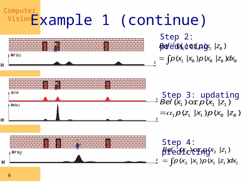
Example 1 (continue)
1 1 1
1 1 1 0 0
( ) or ( | )
( | ) ( | )
Bel x p x z
p z x p x z
Step 3: updating
12 2 1
2 1 1 1 1
( ) or ( | )
( | ) ( | )
Bel x p x z
p x x p x z dx
Step 4: predicting
11 1 0
1 0 0 0 0
( ) or ( | )
( | ) ( | )
Bel x p x z
p x x p x z dx
Step 2: predicting

ComputerVision
10
Several types of Bayes filters
• They differs in how to represent probability densities– Kalman filter– Multihypothesis filter– Grid-based approach– Topological approach– Particle filter

ComputerVision
11
Kalman FilterRecall general problem
1( , )
( , )t t t t
t t t t
x f x w
z g x v
Assumptions of Kalman Filter:
1 , where (0, )
, where (0, )t t t t t t
t t t t t t
x A x w w N Q
z C x v v N R
( ) ( : , )t t t tBel x N x Belief of Kalman Filter is actually a unimodal Gaussian
Advantage: computational efficiencyDisadvantage: assumptions too restrictive
ComputerVision
12

ComputerVision
13

ComputerVision
14
Multi-hypothesis Tracking
• Belief is a mixture of Gaussian
• Tracking each Gaussian hypothesis using a Kalman filter• Deciding weights on the basis of how well the
hypothesis predict the sensor measurements• Advantage:
– can represent multimodal Gaussian• Disadvantage:
– Computationally expensive– Difficult to decide on hypotheses
( ) ~ ( : , )i i it t t t t
i
Bel x w N x
ComputerVision
15
Grid-based Approaches
• Using discrete, piecewise constant representations of the belief
• Tessellate the environment into small patches, with each patch containing the belief of object in it
• Advantage:– Able to represent arbitrary distributions over the
discrete state space• Disadvantage
– Computational and space complexity required to keep the position grid in memory and update it
ComputerVision
16
Topological approaches
• A graph representing the state space– node representing object’s location (e.g. a
room)– edge representing the connectivity (e.g.
hallway)• Advantage
– Efficiency, because state space is small • Disadvantage
– Coarseness of representation

ComputerVision
17
Particle filters
• Also known as Sequential Monte Carlo Methods • Representing belief by sets of samples or
particles
are nonnegative weights called importance factors
• Updating procedure is sequential importance sampling with re-sampling
( ) ~ { , | 1,..., }i it t t tBel x S x w i n
itw

ComputerVision
18
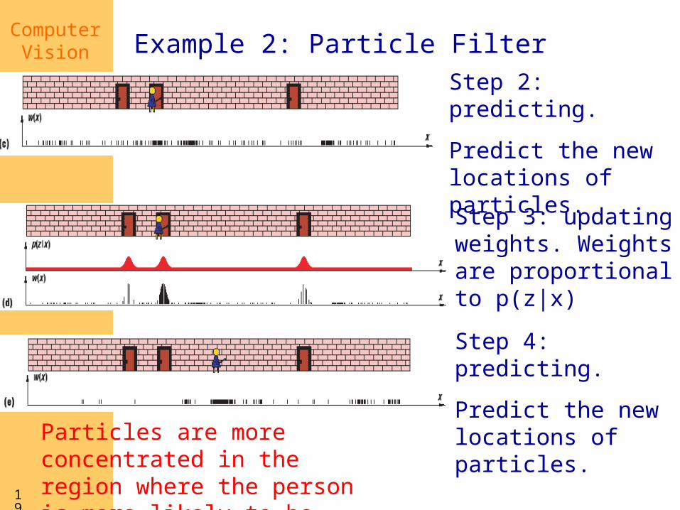
Example 2: Particle Filter
Step 0: initialization
Each particle has the same weight
Step 1: updating weights. Weights are proportional to p(z|x)
ComputerVision
19
Example 2: Particle Filter
Particles are more concentrated in the region where the person is more likely to be
Step 3: updating weights. Weights are proportional to p(z|x)
Step 4: predicting.
Predict the new locations of particles.
Step 2: predicting.
Predict the new locations of particles.
ComputerVision
20
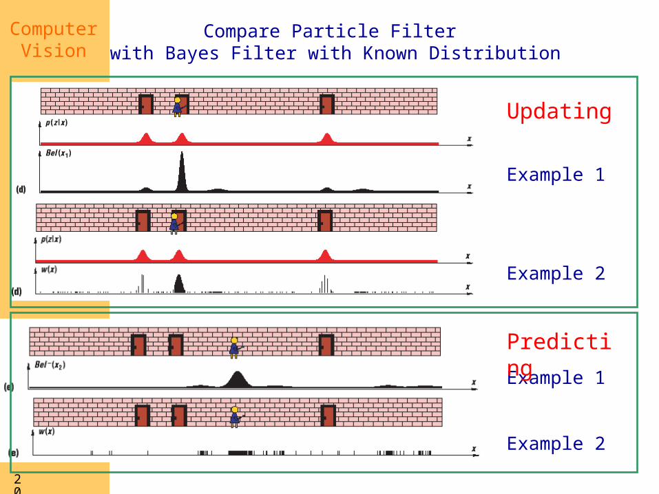
Compare Particle Filter with Bayes Filter with Known Distribution
Example 1
Example 2
Example 1
Example 2
Predicting
Updating

ComputerVision
21
Comments on Particle Filters
• Advantage:– Able to represent arbitrary density– Converging to true posterior even for non-
Gaussian and nonlinear system– Efficient in the sense that particles tend to focus
on regions with high probability
• Disadvantage– Worst-case complexity grows exponentially in the
dimensions

ComputerVision
22
Particle Filtering in CV: Initial Particle Set
• Particles at t = 0 drawn from wide prior because of large initial uncertainty– Gaussian with large
covariance– Uniform distribution
from MacCormick & Blake, 1998
State includes shape & position;prior more constrained for shape

ComputerVision
23
• Normalize N particle weights so that they sum to 1
• Resample particles by picking randomly and
uniformly in [0, 1] range N times– Analogous to spinning a roulette
wheel with arc-lengths of bins equal to particle weights
• Adaptively focuses on promising areas of state space
Particle Filtering: Sampling
¼(1)
¼(2)
¼(3)
¼(N)
¼(N-1)
courtesy of D. Fox
ComputerVision
24
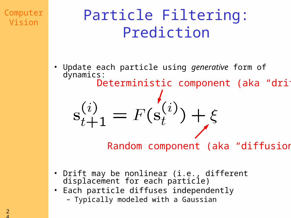
Particle Filtering: Prediction
• Update each particle using generative form of dynamics:
• Drift may be nonlinear (i.e., different displacement for each particle)
• Each particle diffuses independently– Typically modeled with a Gaussian
Random component (aka “diffusion”)
Deterministic component (aka “drift”)
ComputerVision
25
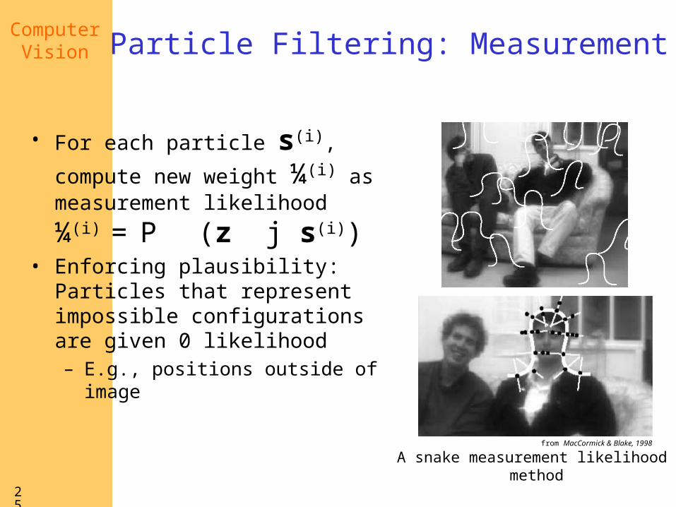
Particle Filtering: Measurement
• For each particle s(i), compute
new weight ¼(i) as
measurement likelihood ¼(i) =
P (z j s(i))• Enforcing plausibility: Particles
that represent impossible configurations are given 0 likelihood– E.g., positions outside of image
from MacCormick & Blake, 1998
A snake measurement likelihood method

ComputerVision
26
Particle Filtering Steps (aka CONDENSATION)
drift
diffuse
measure
measurementlikelihood
from Isard & Blake, 1998
Sampling occurshere
ComputerVision
27
Particle Filtering Visualization
courtesy of M. Isard
1-D system, red curve is measurement likelihood

ComputerVision
28
CONDENSATION: Example State Posterior
from Isard & Blake, 1998
Note how initial distribution “sharpens”
ComputerVision
29
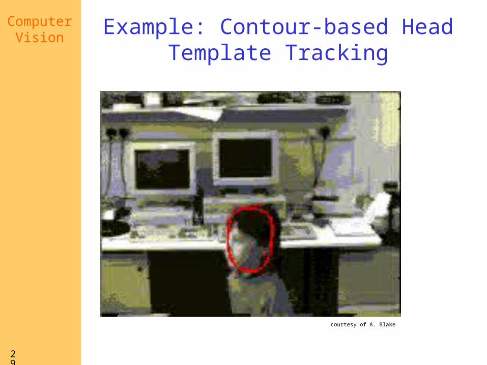
Example: Contour-based Head Template Tracking
courtesy of A. Blake

ComputerVision
30
Example: Recovering from Distraction
from Isard &Blake, 1998
ComputerVision
31
Obtaining a State Estimate
• Note that there’s no explicit state estimate maintained—just a “cloud” of particles
• Can obtain an estimate at a particular time by querying the current particle set
• Some approaches– “Mean” particle
• Weighted sum of particles• Confidence: inverse variance
– Really want a mode finder—mean of tallest peak
ComputerVision
32
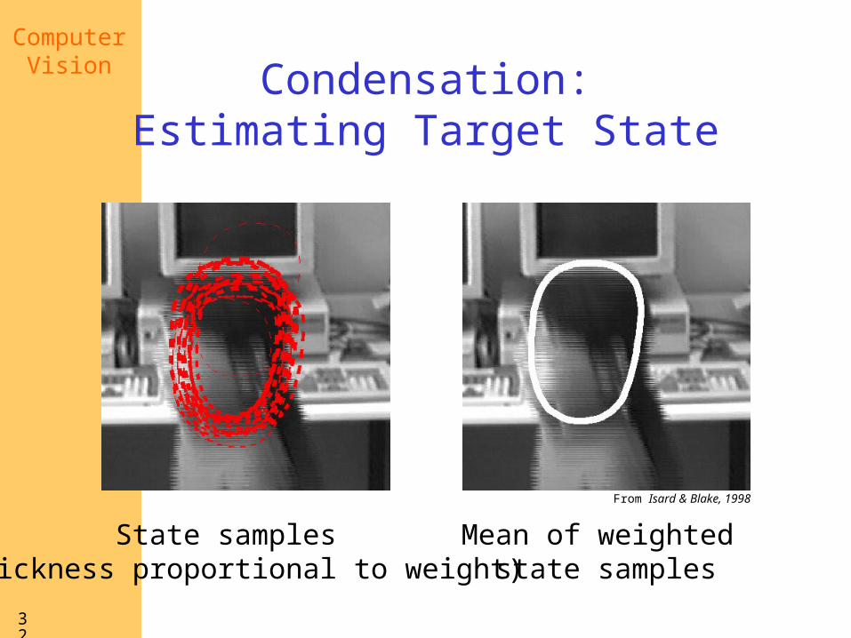
Condensation:Estimating Target State
From Isard & Blake, 1998
State samples (thickness proportional to weight)
Mean of weighted state samples
ComputerVision
33
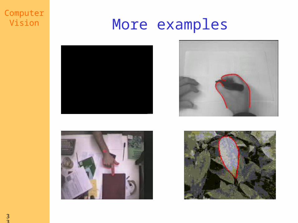
More examples
ComputerVision
34
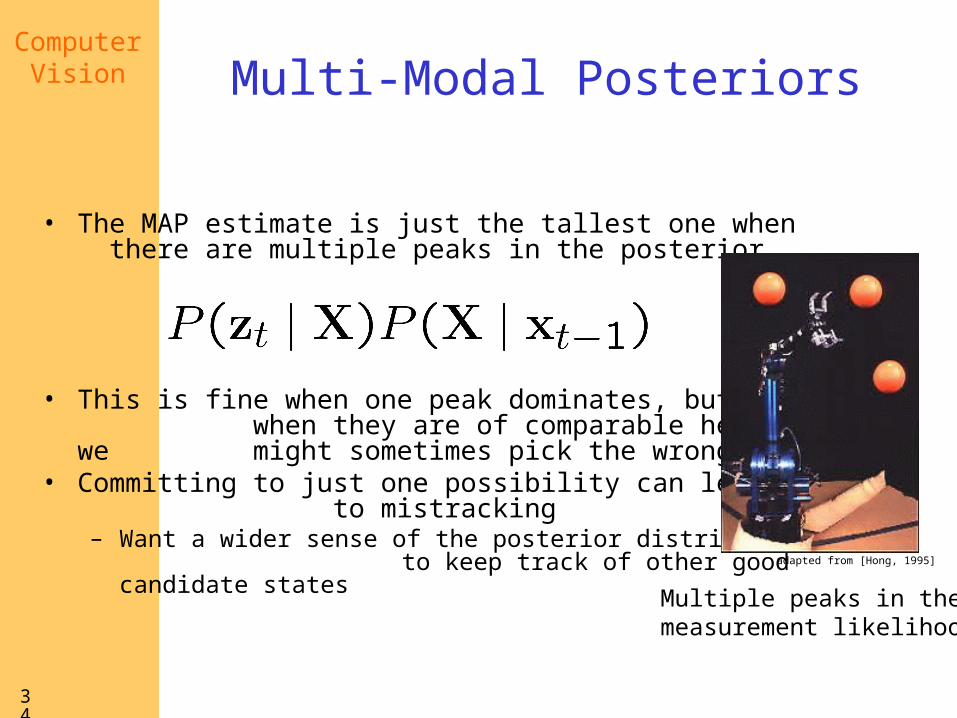
Multi-Modal Posteriors
• The MAP estimate is just the tallest one when there are multiple peaks in the posterior
• This is fine when one peak dominates, but when they are of comparable heights, we might sometimes pick the wrong one
• Committing to just one possibility can lead to mistracking – Want a wider sense of the posterior distribution
to keep track of other good candidate states adapted from [Hong, 1995]
Multiple peaks in the measurement likelihood
ComputerVision
35
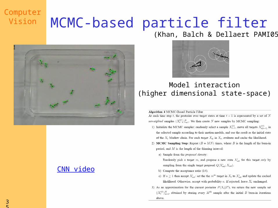
MCMC-based particle filter
Model interaction(higher dimensional state-space)
CNN video
(Khan, Balch & Dellaert PAMI05)

ComputerVision
36
Next class: recognition
Top Related