


![The Dynamical Casimir Effect · 2012. 8. 9. · The Casimir effect The static Casimir effect Vacuum fluctuations [2] Casimir force between two metal plates [2] Two static mirrors](https://static.fdocuments.net/doc/165x107/60fba485759e576738445374/the-dynamical-casimir-effect-2012-8-9-the-casimir-effect-the-static-casimir.jpg)
Languages
Pages
Legal

COMPARISON OF CASIMIR, ELASTIC, ELECTROSTATIC FORCES FOR A MICRO-CANTILEVER
by
AMMAR ALHASAN B.S. AL-Mustansiry University, 2008
A thesis submitted in partial fulfillment of the requirements for the degree of Masters of Science
in the Department of Physics in the College of Science
at the University of Central Florida Orlando, Florida
Spring Term 2014
Major Professor: Robert E. Peale

©2014 Ammar Alhasan
ii
ABSTRACT
Casimir force is a cause of stiction (adhesion) between metal surfaces in Micro-
Electro Mechanical Systems (MEMS). Casimir Force depends strongly on the separation
of the two surfaces and the contact area. This thesis reviews the theory and prior
experimental demonstrations of the Casimir force. Then the Casimir attractive force is
calculated for a particular MEMS cantilever device, in which the metal cantilever tip is
required to repeatedly touch and release from a metal tip pad on the substrate surface in
response to a periodic driving electrostatic force. The elastic force due to the bending of
the cantilever support arms is also a consideration in the device operation. The three
forces are calculated analytically and compared as a function of cantilever tip height.
Calculation of the electrostatic force uses coefficients of capacitance and electrostatic
induction determined numerically by the finite element method, including the effect of
permittivity for the structural oxide. A condition on the tip area to allow electrostatic
release of the tip from the surface against Casimir sticking and elastic restoring forces is
established.
iii

Dedicated to:
HCED Iraq and my parents
iv
ACKNOWLEDMENTS
Words cannot describe the gratitude that I have for my advisor Dr. Robert Peale.
Without his help and guidance, this thesis could never have been accomplished. He has
assisted in every aspect of my research and I am truly grateful for allowing me to work in
his research group,
I would also like to warmly thank Dr. Enrique Del Barco and Dr. Lee Chow for
serving on my thesis committee and taking the time reading and evaluating my thesis and
providing me with invaluable insight.
I would also like to acknowledge Imen Rezadad for his role in assisting me in
various technical aspects of my research especially to learn how to work on the
simulation by using Elmer program. Also, thanks to Evan Smith and Javaneh
Boroumand for their assistance on introducing me to the proper techniques to work with
and maintain equipment related to my research. Working with them, and learning from
their experience has been extremely beneficial for me. I would also thank Mehmet
Yesiltas for his helping in digitizing the data. Throughout my research I have been
blessed enough to receive great suggestions and comments from my group members and
my friends and I want to thank all of them. Also I would thank my parents who have been
supporting me. I wish to acknowledge my government and the program HCED for
supporting me during all these years and giving me the opportunity to advance my
academic career in the United States. Above all, I give thanks to God for all the good
things that I have learned.
v
TABLE OF CONTENTS
LIST OF FIGURES ............................................................................................. viii
INTRODUCTION .................................................................................................. 1
CHAPTER ONE: THEORETICAL CONSIDERATIONS .................................... 4
CHAPTER TWO: REVIEW OF PRIOR CASIMIR FORCE INVESTIGATIONS
............................................................................................................................................. 7
M.J Sparnaay. Attractive Forces between Flat Plates ......................................... 7
Bressi et al. Measurement of the Casimir Force between Parallel Metallic
Surfaces ........................................................................................................................... 8
U. Mohideen. Precision Measurement of the Casimir Force from 0.1 to 0.9 μm
....................................................................................................................................... 10
J.Munday. Measured long-range repulsive Casimir–Lifshitz forces ................ 12
Ricardo. Measurement of the Casimir Force using a micromechanical torsional
oscillator: Electrostatic Calibration ............................................................................... 14
CHAPTER THREE: ESTIMATION OF CASIMIR FORCE FOR HypIR
CANTILEVER ................................................................................................................. 17
Electrostatic force ............................................................................................. 21
CHAPTER FOUR: FORCE OPTIMIZATION .................................................... 26
CHAPTER FIVE: SUMMARY ............................................................................ 31
vi
APPENDIX A: EIGEN FREQUENCIES OF A CUBOIDAL RESONATOR
WITH PERFICTLY CONDUCTING WALLS................................................................ 33
APPENDIX B: EULER -MACLAURIN FORMULA ......................................... 36
LIST OF REFRENCES ........................................................................................ 39
vii
LIST OF FIGURES
Figure 1: Two metal plates are closely spaced. The number of modes outside the
plates is large because the volume is large. The number of modes in the space between
the plates is smaller because fewer modes can satisfy the boundary conditions. Thus the
radiation pressure on the outer plate surfaces exceeds that on the inner surfaces, resulting
in an attraction..................................................................................................................... 2
Figure 2: Experimental set up of Bressi et al [8]. ................................................... 9
Figure 3: Square of the frequency shift as a function of separation for the
experiment of Bressi et al [8]. ........................................................................................... 10
Figure 4: Schematic of metallized sphere mounted on an AFM cantilever above
metal plate [9]. .................................................................................................................. 11
Figure 5: Force as a function of the distance moved by the plate. The solid line is
the theoretical Casimir force. Experimental data are represented by square symbols [9].
........................................................................................................................................... 12
Figure 6: Measured repulsive (open circles) or attractive (solid square) Casimir
force between a gold-coated (100 nm) polystyrene sphere and silica or gold-coated plate
immersed in bromobenzene [5]. ...................................................................................... 14
Figure 7: Schematic of experiment of Ref. [10]. ................................................. 15
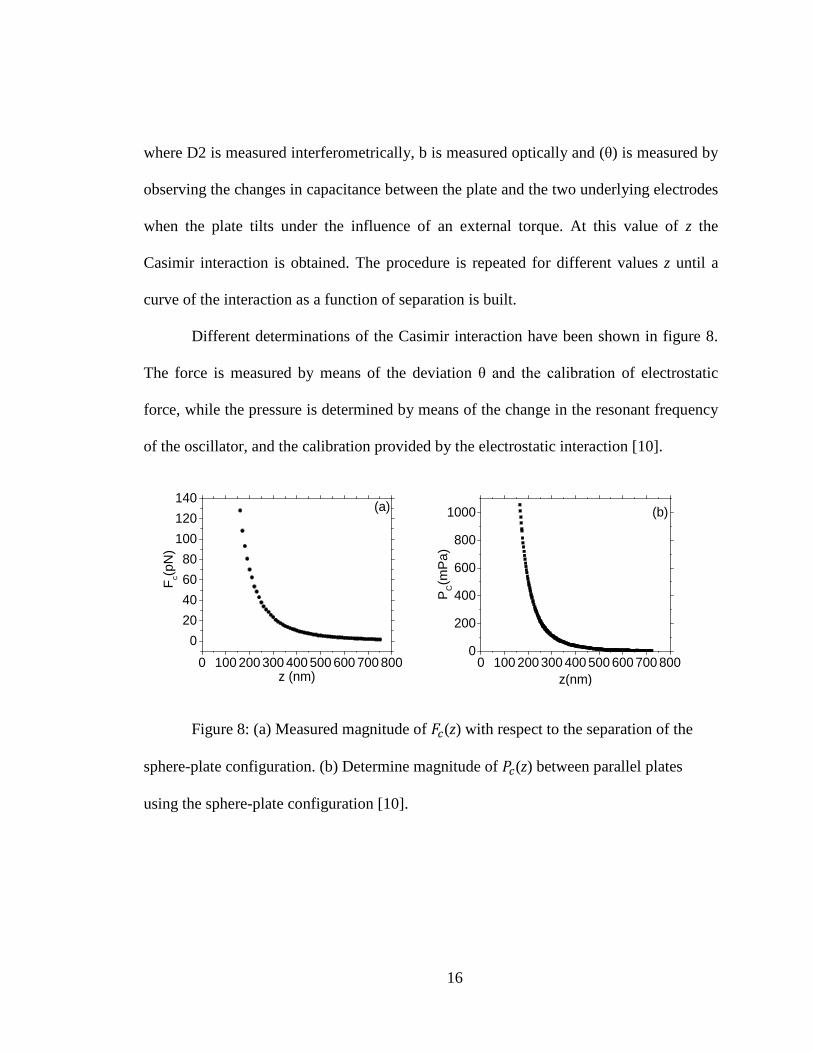
Figure 8: (a) Measured magnitude of 𝐹𝐹𝐹𝐹(z) with respect to the separation of the
sphere-plate configuration. (b) Determine magnitude of 𝑃𝑃𝐹𝐹(z) between parallel plates
using the sphere-plate configuration [10]. ........................................................................ 16
Figure 9: SEM image of MEMS cantilever with tip contact. ............................... 17
viii
Figure 10: SEM image of MEMS cantilever with 18 µm x 18 µm paddle. ......... 18
Figure 11: Log-Log plot comparing Casimir, Elastic, and Electrostatic forces with
respect to tip height z. ....................................................................................................... 20
Figure 12: Schematic of model device for calculation purposes. The electrostatic
portion of the device consists of three parallel plates with 18 µm x 18 µm dimensions.
These are a fixed buried plate (1), a fixed surface plate (2), and a moveable cantilever (3).
The separation of the surface plate and cantilever metal is ζ and has the minimum value
0.5 µm due to the structural oxide. The separation of the tip and tip contact is z. .......... 22
Figure 13: The capacitance and electrostatic induction coefficients with respect to
the separation ζ. The inset presents a log-log plot for three of the coefficients. ............. 23
Figure 14: Electrostatic force vs. ζ for the maximum permissible applied bias of
40 V. .................................................................................................................................. 24
Figure 15: the capacitance and the electrostatic inductions vs. the gap ζ. ............ 26
Figure 16: Coefficients of capacitance and of electrostatic induction with strong
dependence on cantilever displacement. The three terms with (without) subscript “ox”
are the results of calculations for devices with (without) oxide. ...................................... 27
Figure 17: Electrostatic repulsive force vs. ζ with and without the structural oxide.
........................................................................................................................................... 28
Figure 18: Log-Log plot comparing Casimir, Elastic, and Electrostatic forces,
with oxide included, as a function of tip height z, for tip area 2 µm x 2 µm. ................... 29
Figure 19: Log-Log plot of Casimir, Elastic, and Electrostatic forces vs. the tip
height z for tip area 25 nm x 25 nm. ................................................................................. 30
ix
INTRODUCTION
Quantum electrodynamics (QED) predicts a force between two closely spaced
objects due to quantum electromagnetic fluctuations. For metals, the force was first
studied by Casimir (1948) and is hence known as the Casimir force. Two perfectly
conducting, uncharged, closely spaced, parallel flat plates in vacuum attract due to
exclusion of electromagnetic modes between them. This is a purely quantum-mechanical
effect arising from the zero-point energy of the harmonic oscillators that are the normal
modes of the electromagnetic field [1]. The Casimir force depends on geometry [2].
Casimir force becomes large at small separations, equaling ~1 atmosphere of pressure at
10 nm separation [3].
Fig. 1 explains qualitatively the origin of the Casimir force. The number of
different frequencies per unit frequency interval is V ω2/2π2c3 [4], i.e. it is proportional to
volume. As the volume between to metal places decreases, fewer modes are supported in
comparison to the number of modes outside the plates. Thus, the radiation on the inner
surfaces of the conduction plates is less. Fig. 1 suggests this schematically by showing
that the space between the plates supports only short wavelength modes, while the space
outside supports additional long-wavelength ones.
1
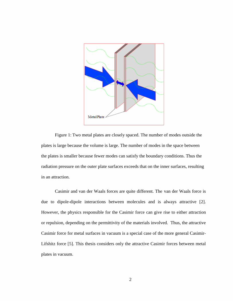
Figure 1: Two metal plates are closely spaced. The number of modes outside the
plates is large because the volume is large. The number of modes in the space between
the plates is smaller because fewer modes can satisfy the boundary conditions. Thus the
radiation pressure on the outer plate surfaces exceeds that on the inner surfaces, resulting
in an attraction.
Casimir and van der Waals forces are quite different. The van der Waals force is
due to dipole-dipole interactions between molecules and is always attractive [2].
However, the physics responsible for the Casimir force can give rise to either attraction
or repulsion, depending on the permittivity of the materials involved. Thus, the attractive
Casimir force for metal surfaces in vacuum is a special case of the more general Casimir-
Lifshitz force [5]. This thesis considers only the attractive Casimir forces between metal
plates in vacuum.
2
Casimir force is usually very weak compared with electric forces except at very
small distances. It may be strong compared to gravitational force as in MEMS where the
latter force scales as volume and is completely negligible. The importance of surface
effects (e.g. Casimir force) to volume effects (gravitational force) grows as 1/L with
decreasing length scale L.
3

CHAPTER ONE: THEORETICAL CONSIDERATIONS
We consider the zero point electromagnetic energy in a box, which is assumed to
be a rectangular parallelepiped with perfectly conducting walls of area L x L and
separation d. Electromagnetic waves inside the box must have nodes on the walls, which
restricts and discretizes the possible frequencies. This causes a dependence on the wall
separation d of the zero point energy, which results in a force on the walls. Smaller
volume between the walls causes smaller the zero point energy, so that energy is lowered
when the walls move closer. Thus, the force is attractive
The boundary conditions require that integral numbers of half wavelengths exist
between each pair of walls. For example, the wavelength of an electromagnetic wave
traveling (e.g.) in the short direction of the box must satisfy nλ/2 = d, giving a wave
vector kz = nπ/d, where n is an integer. Taking into account all possible propagation
directions, the allowed frequencies are
𝜔𝜔𝑙𝑙𝑙𝑙𝑙𝑙 = 𝜋𝜋𝐹𝐹(𝑙𝑙2
𝐿𝐿2+ 𝑙𝑙2
𝐿𝐿2+ 𝑙𝑙2
𝑑𝑑2)12 (1. 1 )
where each mode is enumerated by three positive integers l, m, and n. The
electromagnetic field is quantized with energy
E = ∑ 2ħωl,m,n(𝑁𝑁𝑙𝑙𝑙𝑙𝑙𝑙 + 12)l,m,n (1. 2 )
Where Nlmn is the number of quanta in the lmnth mode. The factor of 2 accounts
for two-fold degeneracy of every frequency for which all the l,m,n are non-zero
(Appendix A). The zero point energy corresponds to zero quanta in any mode, or
4

E0 = ∑ ħωl,m,nl,m,n = ∑ ħ𝐹𝐹(𝑙𝑙2𝜋𝜋2
𝐿𝐿2+ 𝑙𝑙2𝜋𝜋2
𝐿𝐿2+ 𝑙𝑙2𝜋𝜋2
𝑑𝑑2)12,
𝑙𝑙,𝑙𝑙,𝑙𝑙 (1. 3 )
The prime indicates that when one of these integers is equal to zero there should be a
factor one half because such frequencies are non-degenerate (Appendix A). When two of
the integers are zero, there is no electric field at all (Appendix A).
Because L >> d, the density of modes is much larger in the transverse directions
than in the longitudinal direction of the cavity, so that the sums over indices l and m may
be converted to integrals over wavenumbers, using 𝑑𝑑𝑑𝑑𝑥𝑥 = 𝜋𝜋𝐿𝐿𝑑𝑑𝑑𝑑 , etc.
𝐸𝐸0(𝑑𝑑) = ħ𝑐𝑐𝐿𝐿2
𝜋𝜋2∑ ∫ 𝑑𝑑𝑑𝑑𝑥𝑥
∞0
,𝑙𝑙 ∫ 𝑑𝑑𝑑𝑑𝑦𝑦
∞0 (𝑑𝑑𝑥𝑥2 + 𝑑𝑑𝑦𝑦2 + 𝑙𝑙2𝜋𝜋2
𝑑𝑑2)12 (1. 4 )
For large plate separations, the sum over n is similarly replaced by an integral giving 𝐸𝐸0(∞) = ħ𝑐𝑐𝐿𝐿2𝑑𝑑
𝜋𝜋3 ∭ (𝑢𝑢2 + 𝑣𝑣2 + 𝑤𝑤2)12
∞0 𝑑𝑑𝑢𝑢𝑑𝑑𝑣𝑣𝑑𝑑𝑤𝑤 (1. 5 )
The energy required to bring the plates from a large distance to a separation d is U (d)= 𝐸𝐸0(𝑑𝑑) − 𝐸𝐸0(∞)
= ħ𝑐𝑐𝐿𝐿2
𝜋𝜋2[∑ ∬ (𝑢𝑢2 + 𝑣𝑣2 + 𝜋𝜋2𝑙𝑙2
𝑑𝑑2)12
∞0
,𝑙𝑙 𝑑𝑑𝑢𝑢𝑑𝑑𝑣𝑣 − 𝑑𝑑
𝜋𝜋∭ (𝑢𝑢2 + 𝑣𝑣2 + 𝑤𝑤2)12
∞0 𝑑𝑑𝑢𝑢𝑑𝑑𝑣𝑣𝑑𝑑𝑤𝑤 (1. 6 )
Transforming to cylindrical polar coordinates (u2 + v2 = r2, dudv = r dr d𝜃𝜃), with
the integral over θ giving π/2 since the original integral is over positive values of u and v
only, gives
U (d)= ħ𝑐𝑐𝐿𝐿2
2𝜋𝜋 [∑ ∫ (𝑟𝑟2∞
0∞𝑙𝑙=0 + 𝑙𝑙2𝜋𝜋2
𝑑𝑑2)12𝑟𝑟𝑑𝑑𝑟𝑟 − 𝑑𝑑
𝜋𝜋 ∫ 𝑑𝑑𝑤𝑤 ∫ (𝑟𝑟2 + 𝑤𝑤2)
12𝑟𝑟𝑑𝑑𝑟𝑟∞
0∞0 ] (1. 7 )
In the second integral, substitute 𝑤𝑤 , = 𝑑𝑑𝜋𝜋𝑤𝑤, and then drop the primes to get
U (d)= ħ𝑐𝑐𝐿𝐿2
2𝜋𝜋 �∑ ∫ (𝑟𝑟2∞
0∞𝑙𝑙=0 + 𝜋𝜋2
𝑑𝑑2𝑑𝑑2�
12 𝑟𝑟𝑑𝑑𝑟𝑟 − ∫ 𝑑𝑑𝑤𝑤 ∫ �𝑟𝑟2 + 𝜋𝜋2
𝑑𝑑2𝑤𝑤2�
12 𝑟𝑟𝑑𝑑𝑟𝑟∞
0∞0 ] (1. 8 )
5
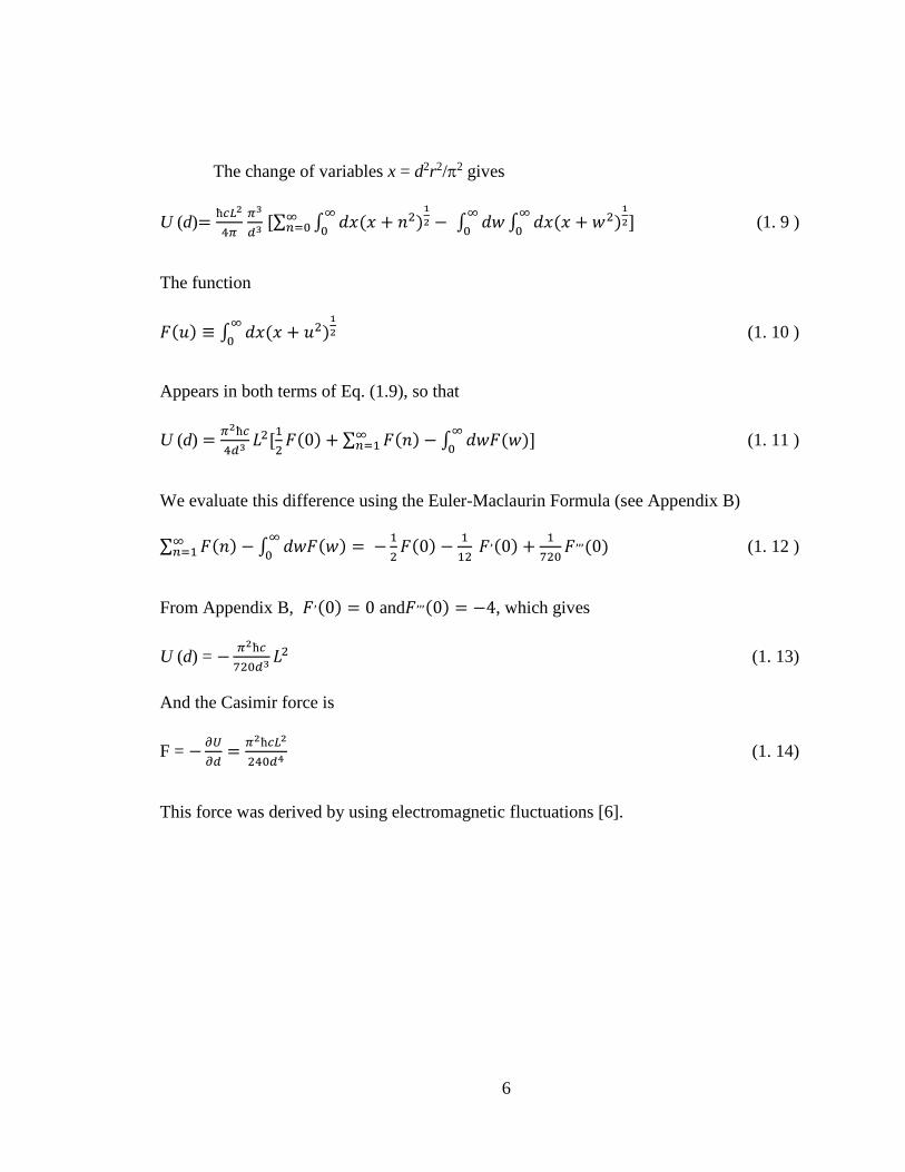
The change of variables x = d2r2/π2 gives
U (d)= ħ𝑐𝑐𝐿𝐿2
4𝜋𝜋 𝜋𝜋
3
𝑑𝑑3 [∑ ∫ 𝑑𝑑𝑑𝑑(𝑑𝑑∞
0∞𝑙𝑙=0 + 𝑑𝑑2)
12 − ∫ 𝑑𝑑𝑤𝑤 ∫ 𝑑𝑑𝑑𝑑(𝑑𝑑 + 𝑤𝑤2)
12
∞0
∞0 ] (1. 9 )
The function
𝐹𝐹(𝑢𝑢) ≡ ∫ 𝑑𝑑𝑑𝑑(𝑑𝑑 + 𝑢𝑢2∞0 )
12 (1. 10 )
Appears in both terms of Eq. (1.9), so that
U (d) = 𝜋𝜋2ħ𝑐𝑐4𝑑𝑑3
𝐿𝐿2[12𝐹𝐹(0) + ∑ 𝐹𝐹(𝑑𝑑) − ∫ 𝑑𝑑𝑤𝑤𝐹𝐹(𝑤𝑤)]∞
0∞𝑙𝑙=1 (1. 11 )
We evaluate this difference using the Euler-Maclaurin Formula (see Appendix B) ∑ 𝐹𝐹(𝑑𝑑) − ∫ 𝑑𝑑𝑤𝑤𝐹𝐹(𝑤𝑤) = −1
2∞0
∞𝑙𝑙=1 𝐹𝐹(0) − 1
12 𝐹𝐹,(0) + 1
720𝐹𝐹,,,(0) (1. 12 )
From Appendix B, 𝐹𝐹,(0) = 0 and𝐹𝐹,,,(0) = −4, which gives
U (d) = − 𝜋𝜋2ħ𝑐𝑐720𝑑𝑑3
𝐿𝐿2 (1. 13)
And the Casimir force is
F = −𝜕𝜕𝜕𝜕𝜕𝜕𝑑𝑑
= 𝜋𝜋2ħ𝑐𝑐𝐿𝐿2
240𝑑𝑑4 (1. 14)
This force was derived by using electromagnetic fluctuations [6].
6
CHAPTER TWO: REVIEW OF PRIOR CASIMIR FORCE INVESTIGATIONS
M.J Sparnaay. Attractive Forces between Flat Plates
The earliest attempt to measure the Casimir force was published in 1957 by
Sparnaay [6], nine years after Casimir’s paper. Parallel metal plates were used. The main
difficulty in getting the plates close and pararallel was dust particles on the surfaces. Two
aluminum parallel plates were used. One of them could be moved by using lever system.
The other was attached to a spring system. The attractive force K was measured by using
capacity methods, but the “surfaces asperities” prevented accurate measurement of the
force.
If instead, two chromium or chromium-steel plates were used, the measurements
indicated that Casimir’s relation K=A𝑑𝑑−4 was not contradicted. The constant A was
found to have a value in the range 0.01 to 0.04×10⁻¹⁶dynes 𝐹𝐹𝑐𝑐2, whereas the theoretical
value is 0.013×10⁻¹⁰ dynes 𝐹𝐹𝑐𝑐2. The very large difference was attributed to the
determination of the parallelism of the plates, whose separation was varied from 0.3 μm
to 2 μm.
The materials of the two plates were chosen to be identical metals, because
different metals would have different surfaces potentials and would attract each other
according to 𝐾𝐾1=4.4 ×10⁻⁵𝑃𝑃2 𝑑𝑑−2, where P is the potential difference in millivolts and d
is the separation in microns. The two plates were insulated so that the time constant (RC)
of the discharge was much larger than one second. This required R≫ 109 Ohm [7].
7
Bressi et al. Measurement of the Casimir Force between Parallel Metallic Surfaces
Bressi et al. (2002) measured Casimir force between parallel metallic surfaces [8],
Fig. 2. One of these was a cantilever beam (resonator) that was free to oscillate around
its holding point. A second beam (source) was connected to a frame whose distance to
the cantilever was controlled by a piezoelectric transducer (PZT). The silicon cantilever
and the source were mounted within a vacuum chamber at a pressure of ~10−5 mbar.
The cantilever size was 1.9 cm x 1.2 mm x 47 µm with average roughness 10 nm. It was
coated with a 50-nm-thick chromium layer and was fixed to a copper base. The source
had the same “longitudinal” dimensions except for its thickness, which was 0.5 mm. It
could be rotated by stepping motors around two axes to finely control the parallelism of
the opposing surfaces. The source and the resonator were electrically connected to a
voltage calibrator for the electrostatic calibrations. Alternatively, they were connected to
an AC bridge for measuring the capacitance and for alignment by maximizing this
capacitance at the minimum obtainable gap separation. The optical interferometer
detected and quantified the motion of the cantilever [8].
8

Figure 2: Experimental set up of Bressi et al [8].
The attractive Casimir force shifts the resonance frequency. The shift was
measured as a function of separation over the range 0.5- 3.0 μm. The square of the shift
is plotted as samples vs separation in Fig. 3. A residual electrostatic force contribution
was zeroed by a dynamic technique. The result is shown in Fig.3 with the best fit with the
function (2.1)
∆𝜈𝜈2(𝑑𝑑) = −𝐶𝐶𝑐𝑐𝑐𝑐𝑑𝑑5
(2.1)
The experimental verification of the Casimir prediction for the force between two parallel
conducting surfaces in the 0.5 - 3.0 μm range leads to a measurement of the related
coefficient with 15% precision.
9

Figure 3: Square of the frequency shift as a function of separation for the
experiment of Bressi et al [8].
U. Mohideen. Precision Measurement of the Casimir Force from 0.1 to 0.9 μm
Mohideen characterized the Casimir force using an atomic force microscope
(AFM) [9]. The experiment consisted of a metallized sphere of diameter 196 μm and a
flat plate. This arrangement has the advantage over parallel plates of not requiring
alignment. The separation varied from 0.1 to 0.9 μm. The experiment was done at room
temperature in vacuum at 50 mTorr pressure. The sphere was mounted on the tip of 300
μm long cantilever with Ag epoxy. A 1.25 cm diameter optically polished disk was used
as the plate. The cantilever, the plate, and the sphere were coated with 300 nm of Al in an
evaporator. Aluminum only was used on the cantilever because of its high optical
10
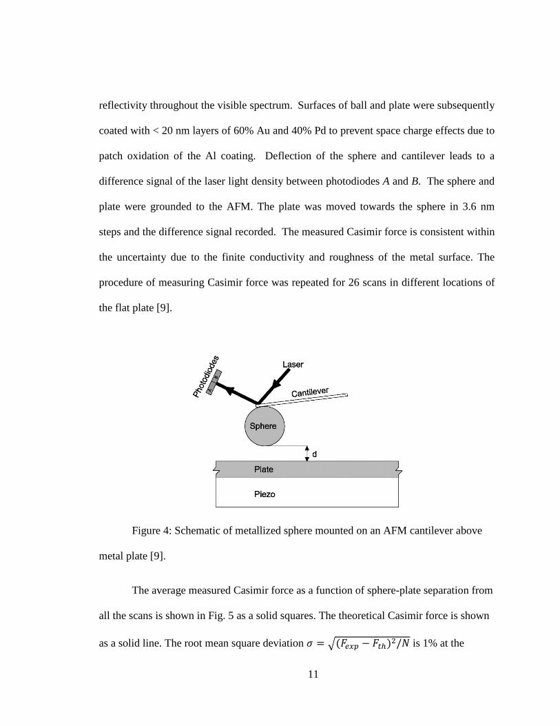
reflectivity throughout the visible spectrum. Surfaces of ball and plate were subsequently
coated with < 20 nm layers of 60% Au and 40% Pd to prevent space charge effects due to
patch oxidation of the Al coating. Deflection of the sphere and cantilever leads to a
difference signal of the laser light density between photodiodes A and B. The sphere and
plate were grounded to the AFM. The plate was moved towards the sphere in 3.6 nm
steps and the difference signal recorded. The measured Casimir force is consistent within
the uncertainty due to the finite conductivity and roughness of the metal surface. The
procedure of measuring Casimir force was repeated for 26 scans in different locations of
the flat plate [9].
Figure 4: Schematic of metallized sphere mounted on an AFM cantilever above
metal plate [9].
The average measured Casimir force as a function of sphere-plate separation from
all the scans is shown in Fig. 5 as a solid squares. The theoretical Casimir force is shown
as a solid line. The root mean square deviation 𝜎𝜎 = �(𝐹𝐹𝑒𝑒𝑥𝑥𝑒𝑒 − 𝐹𝐹𝑡𝑡ℎ)2/𝑁𝑁 is 1% at the
11

smallest surface separation can be taken as a statistical measure of the experimental
precision where N is the number of data points.
Figure 5: Force as a function of the distance moved by the plate. The solid line is
the theoretical Casimir force. Experimental data are represented by square symbols [9].
J.Munday. Measured long-range repulsive Casimir–Lifshitz forces
Long-range repulsive Casimir force between a gold-coated sphere and a silica
plate immersed in bromobenzene was measured. When the silica plate was replaced by a
gold film, the force became attractive (Fig.6). The hydrodynamic force between the
sphere and plate was used to calibrate the cantilever force constant and the surface
separation at contact. A repulsive and attractive force in systems is satisfying the equation
(2.2) [5].
200 400 600 800 1000-120-100
-80-60-40-20
020
Cas
imir
Forc
e (1
0-12 N
)
Plate-sphere separation (nm)
12
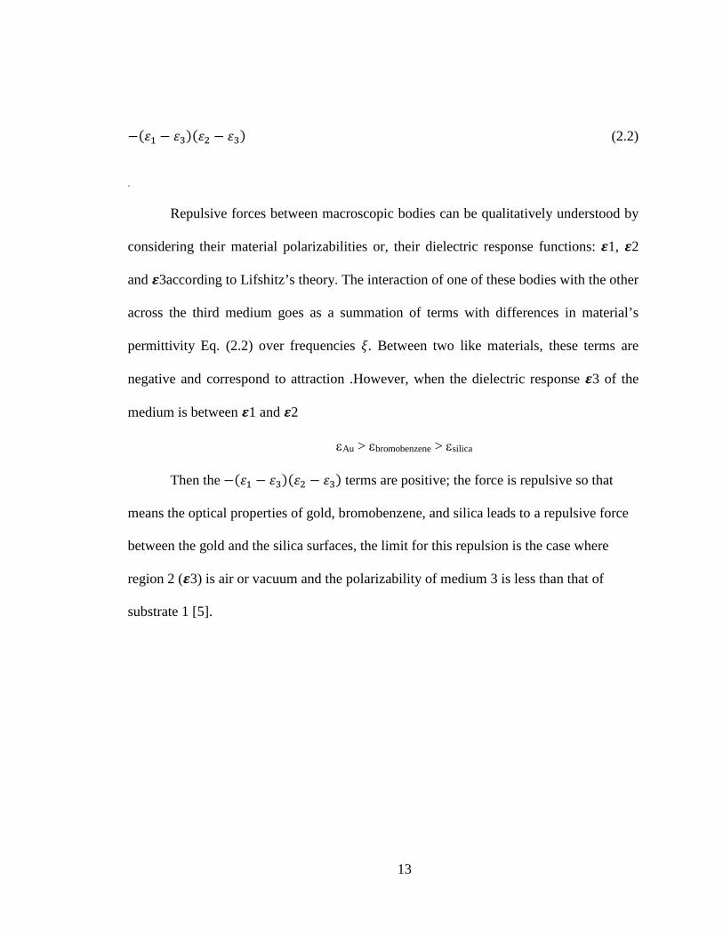
−(𝜀𝜀1 − 𝜀𝜀3)(𝜀𝜀2 − 𝜀𝜀3) (2.2)
.
Repulsive forces between macroscopic bodies can be qualitatively understood by
considering their material polarizabilities or, their dielectric response functions: 𝜺𝜺1, 𝜺𝜺2
and 𝜺𝜺3according to Lifshitz’s theory. The interaction of one of these bodies with the other
across the third medium goes as a summation of terms with differences in material’s
permittivity Eq. (2.2) over frequencies 𝜉𝜉. Between two like materials, these terms are
negative and correspond to attraction .However, when the dielectric response 𝜺𝜺3 of the
medium is between 𝜺𝜺1 and 𝜺𝜺2
εAu > εbromobenzene > εsilica
Then the −(𝜀𝜀1 − 𝜀𝜀3)(𝜀𝜀2 − 𝜀𝜀3) terms are positive; the force is repulsive so that
means the optical properties of gold, bromobenzene, and silica leads to a repulsive force
between the gold and the silica surfaces, the limit for this repulsion is the case where
region 2 (𝜺𝜺3) is air or vacuum and the polarizability of medium 3 is less than that of
substrate 1 [5].
13
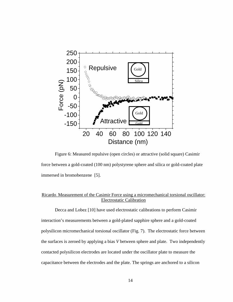
Figure 6: Measured repulsive (open circles) or attractive (solid square) Casimir
force between a gold-coated (100 nm) polystyrene sphere and silica or gold-coated plate
immersed in bromobenzene [5].
Ricardo. Measurement of the Casimir Force using a micromechanical torsional oscillator: Electrostatic Calibration
Decca and Lobez [10] have used electrostatic calibrations to perform Casimir
interaction’s measurements between a gold-plated sapphire sphere and a gold-coated
polysilicon micromechanical torsional oscillator (Fig. 7). The electrostatic force between
the surfaces is zeroed by applying a bias V between sphere and plate. Two independently
contacted polysilicon electrodes are located under the oscillator plate to measure the
capacitance between the electrodes and the plate. The springs are anchored to a silicon
20 40 60 80 100 120 140-150-100
-500
50100150200250
Forc
e (p
N)
Distance (nm)
Attractive
Repulsive
Gold
Gold
Silica
Gold
14

nitride covered Si platform. The sphere is glued with conductive epoxy to the side of an
Au-coated optical fiber, establishing an electrical connection between them. The entire
setup is mounted into a can, where a pressure is less than 10−5 Torr.
Figure 7: Schematic of experiment of Ref. [10].
The Casimir interaction between the Au-coated sphere and the Au-coated
polysilicon plate can be performed by using the electrostatic calibrations. After
performing the electrostatic calibrations the potential between the sphere and the plate is
adjusted to be equal to the average residual potential so that electrostatic force is equal to
zero within experimental error. After that the position of the sphere is changed by Δz ∼ 2
nm, as measured by the interferometer. The actual z is calculated using the measured
parameters by means of Eq. (2.3)
z = zmeans − D1 − D2 – b×θ (2.3)
15
where D2 is measured interferometrically, b is measured optically and (θ) is measured by
observing the changes in capacitance between the plate and the two underlying electrodes
when the plate tilts under the influence of an external torque. At this value of z the
Casimir interaction is obtained. The procedure is repeated for different values z until a
curve of the interaction as a function of separation is built.
Different determinations of the Casimir interaction have been shown in figure 8.
The force is measured by means of the deviation θ and the calibration of electrostatic
force, while the pressure is determined by means of the change in the resonant frequency
of the oscillator, and the calibration provided by the electrostatic interaction [10].
Figure 8: (a) Measured magnitude of 𝐹𝐹𝑐𝑐(z) with respect to the separation of the
sphere-plate configuration. (b) Determine magnitude of 𝑃𝑃𝑐𝑐(z) between parallel plates
using the sphere-plate configuration [10].
0 100 200 300 400 500 600 700 8000
20406080
100120140
F c(pN
)
z (nm)
(a)
0 100 200 300 400 500 600 700 8000
200
400
600
800
1000
PC(m
Pa)
z(nm)
(b)
16

CHAPTER THREE: ESTIMATION OF CASIMIR FORCE FOR HypIR CANTILEVER
Figure 9 presents a scanning electron microscope (SEM) image of a MEMS
cantilever device fabricated by our group at UCF. Shown is a single pixel of an infrared
sensor described in [11, 12] and known as “HypIR”. This particular example has
characteristic lateral dimension 100 µm, and it was fabricated by photo-lithography.
Figure 10 presents an SEM image of a smaller pixel fabricated by electron beam
lithography. This device has a paddle with lateral dimension 18 µm. The image clearly
shows a tip at the central part of the paddle end. The tip is fabricated of gold and is
attached to the underside of the paddle. In the image, this tip is in contact with a tip-pad
on the surface, and it is the only part of the cantilever that contacts the surface besides the
anchors at the ends of the folded arms. This is the intended resting unbiased state of the
device, the so-called “null position”.
Figure 9: SEM image of MEMS cantilever with tip contact.
17

Figure 10: SEM image of MEMS cantilever with 18 µm x 18 µm paddle.
When an electric bias is applied, the tip is supposed to lift up from the surface by
electrostatic repulsion. A more complete description of the elastic and electrostatic
forces involved is presented in [11]. The Casimir force will cause there to be required an
additional electric bias to release the tip from the surface. In other words, the Casimir
force tends to make the surface more “sticky” than otherwise. A goal of this thesis is to
estimate that effect. Our theoretical study is limited to the smaller of the two cantilevers
(Fig. 10), for which the tip dimensions are 2 µm x 2 µm.
The separation z between the tip and the tip contact is supposed to be uniform and
to be restricted to the range 2 nm < z < 2 µm. The lower separation limit is determined by
the typical surface roughness of a commercial silicon wafer as determined by atomic
force microscopy [12], and the larger separation limit is according to the intended
18
operational limit. The Casimir force is given by Eq. (1.14), in which L2 is the area of the
plates. Evaluating the constants, we find the force in Newtons to be
F = 5.2 x 10-39 N-m4/z4. (3.1)
The largest value of this force occurs at the 2 nm separation and has the value 0.325 mN
(milliNewton). This is the force that must be overcome by electrostatic repulsion.
The Hyp-IR cantilever is supposed to be touching the surface in equilibrium. To
lift the cantilever tip, the electrostatic force must also overcome the linear elastic
restoring force FE. For a force concentrated at one end of a beam, the spring constant K
has the value 3𝐸𝐸𝐸𝐸𝐿𝐿3
[13], where E is Young’s modulus, I is the area moment of inertia, and
L is the length of the cantilever arms. For the arms, we ignore that they are folded, and
we take the length to be L = 18 µm. The area moment of inertia I = w𝑡𝑡3/12, where w is
the width and t is the thickness of the arms, so that K = 𝐸𝐸.𝑤𝑤.𝑡𝑡3
4𝐿𝐿3. The width of the two arms
together w = 4 µm, and their thickness t = 0.4 µm. Young’s modulus for oxide E = 73
GPa. Thus, we find that K = 0.6 N/m.
The separation at which the elastic restoring force and the Casimir force are equal
is found by setting Eq. (3.1) equal to Hooke’s law. That distance is 24 nm. At this
separation, both downward forces have the magnitude 14 nN. A log-log plot of these two
forces is plotted as a function of z in Fig. 11. Their power law dependences with slopes
of -4 and +1 are evident. Below 24 nm, the Casimir force is the dominant restoring force
that opposes the electrostatic repulsive lifting of the tip.
19
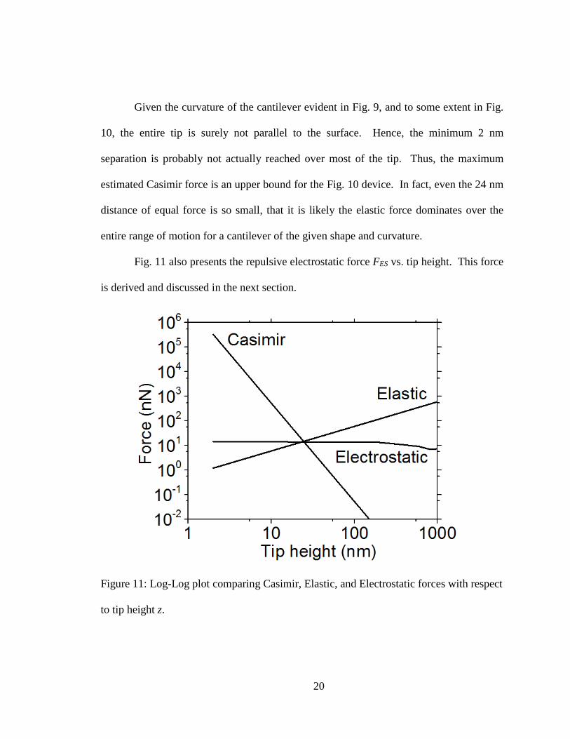
Given the curvature of the cantilever evident in Fig. 9, and to some extent in Fig.
10, the entire tip is surely not parallel to the surface. Hence, the minimum 2 nm
separation is probably not actually reached over most of the tip. Thus, the maximum
estimated Casimir force is an upper bound for the Fig. 10 device. In fact, even the 24 nm
distance of equal force is so small, that it is likely the elastic force dominates over the
entire range of motion for a cantilever of the given shape and curvature.
Fig. 11 also presents the repulsive electrostatic force FES vs. tip height. This force
is derived and discussed in the next section.
Figure 11: Log-Log plot comparing Casimir, Elastic, and Electrostatic forces with respect
to tip height z.
20
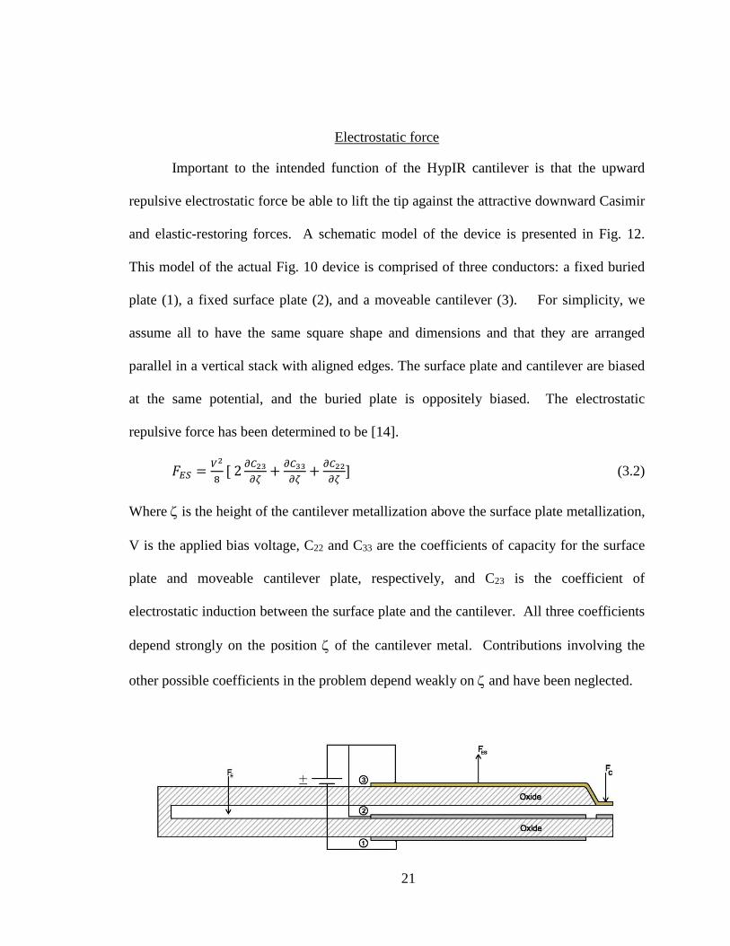
Electrostatic force
Important to the intended function of the HypIR cantilever is that the upward
repulsive electrostatic force be able to lift the tip against the attractive downward Casimir
and elastic-restoring forces. A schematic model of the device is presented in Fig. 12.
This model of the actual Fig. 10 device is comprised of three conductors: a fixed buried
plate (1), a fixed surface plate (2), and a moveable cantilever (3). For simplicity, we
assume all to have the same square shape and dimensions and that they are arranged
parallel in a vertical stack with aligned edges. The surface plate and cantilever are biased
at the same potential, and the buried plate is oppositely biased. The electrostatic
repulsive force has been determined to be [14].
𝐹𝐹𝐸𝐸𝐸𝐸 = 𝑉𝑉2
8[ 2 𝜕𝜕𝐶𝐶23
𝜕𝜕𝜕𝜕+ 𝜕𝜕𝐶𝐶33
𝜕𝜕𝜕𝜕+ 𝜕𝜕𝐶𝐶22
𝜕𝜕𝜕𝜕] (3.2)
Where ζ is the height of the cantilever metallization above the surface plate metallization,
V is the applied bias voltage, C22 and C33 are the coefficients of capacity for the surface
plate and moveable cantilever plate, respectively, and C23 is the coefficient of
electrostatic induction between the surface plate and the cantilever. All three coefficients
depend strongly on the position ζ of the cantilever metal. Contributions involving the
other possible coefficients in the problem depend weakly on ζ and have been neglected.
21
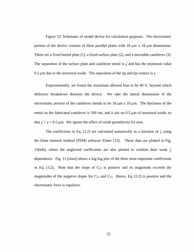
Figure 12: Schematic of model device for calculation purposes. The electrostatic
portion of the device consists of three parallel plates with 18 µm x 18 µm dimensions.
These are a fixed buried plate (1), a fixed surface plate (2), and a moveable cantilever (3).
The separation of the surface plate and cantilever metal is ζ and has the minimum value
0.5 µm due to the structural oxide. The separation of the tip and tip contact is z.
Experimentally, we found the maximum allowed bias to be 40 V, beyond which
dielectric breakdown destroys the device. We take the lateral dimensions of the
electrostatic portion of the cantilever metals to be 18 μm x 18 µm. The thickness of the
metal on the fabricated cantilever is 100 nm, and it sits on 0.5 µm of structural oxide, so
that ζ = z + 0.5 µm. We ignore the effect of oxide permittivity for now.
The coefficients in Eq. (3.2) are calculated numerically as a function of ζ using
the finite element method (FEM) software Elmer [15]. These data are plotted in Fig.
13(left), where the neglected coefficients are also plotted to confirm their weak ζ
dependence. Fig. 13 (inset) shows a log-log plot of the three most important coefficients
in Eq. (3.2). Note that the slope of C23 is positive and its magnitude exceeds the
magnitudes of the negative slopes for C22 and C33. Hence, Eq. (3.2) is positive and the
electrostatic force is repulsive.
22
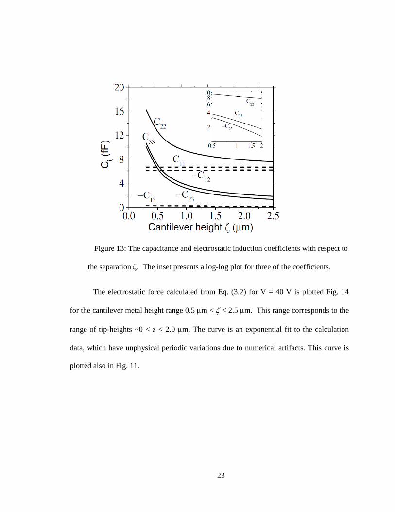
Figure 13: The capacitance and electrostatic induction coefficients with respect to
the separation ζ. The inset presents a log-log plot for three of the coefficients.
The electrostatic force calculated from Eq. (3.2) for V = 40 V is plotted Fig. 14
for the cantilever metal height range 0.5 µm < ζ < 2.5 µm. This range corresponds to the
range of tip-heights ~0 < z < 2.0 µm. The curve is an exponential fit to the calculation
data, which have unphysical periodic variations due to numerical artifacts. This curve is
plotted also in Fig. 11.
23
Figure 14: Electrostatic force vs. ζ for the maximum permissible applied bias of
40 V.
According to Fig. 11, the repulsive electrostatic force is smaller than the Casimir
force below a tip height of z = 24 nm. Accordingly, the tip should not ever lift based
assuming the model design. That the cantilevers of Figs. 9 and 10 have been observed by
video microscopy and electric response [14] to lift from the surface is because they are
non-ideal. Residues and curvature cause the effective minimum separation of tip and tip-
pad to significantly exceed 24 nm.
According to Fig. 11, the electrostatic force is smaller than the elastic restoring
force for values of z > 24 nm. For this reason, too, electrostatic repulsion should fail to
lift the cantilever. That the cantilever does lift indicates that the actual cantilever is
0.0 0.5 1.0 1.5 2.0 2.50
4
8
12
16E
lect
rost
atic
For
ce (n
N)
Cantilever height ζ (µm)
24
longer and floppier than the model, which is not surprising considering that their folded
structure was ignored. Secondly, the electrostatic force is actually distributed over the
cantilever plate (which is itself flexible) and not concentrated at the end of the arms as
assumed. Thirdly, we have ignored the role of the oxide, which will be shown in the next
chapter to give stronger repulsive force.
25

CHAPTER FOUR: FORCE OPTIMIZATION
This chapter considers more realistic calculations, which include the 0.5 μm oxide
layers between buried- and surface-plates and on the underside of the cantilever. The
minimum air gap was taken to be zero. The coefficients of capacity and electrostatic
induction are plotted in Fig. 15 as a function of ζ. In comparison with Fig. 13, the
magnitudes of all the coefficients of the capacitance are increased by the presence of the
oxide layers.
Figure 15: the capacitance and the electrostatic inductions vs. the gap ζ.
The three coefficients of most importance to the force in Eq. (3.2) are plotted in
Fig. 16 and compared with those lacking oxide. The effect of oxide is most noticeable at
small ζ. At large ζ, the curves for C33 with and without oxide, and similarly for C23,
approach each other.
0.5 1.0 1.5 2.0 2.5
0
10
20
30
40
50
C ij (fF)
Cantilever height ζ (µm)
C22
C11
-C12
-C13
-C23
C33
26

Figure 16: Coefficients of capacitance and of electrostatic induction with strong
dependence on cantilever displacement. The three terms with (without) subscript “ox”
are the results of calculations for devices with (without) oxide.
Fig. 17 presents the electrostatic force calculated from Eq. (3.2) and compares
it to the results without oxide. Electrostatic force is higher with oxide, especially at small
ζ. The difference is a factor of 3.9 at ζ = 0.5 µm.
0.5 1.0 1.5 2.0 2.5-30
-15
0
15
30
45
60C
ij (fF
)
Cantilever height ζ (µm)
C22,ox
C33,ox
C22C33
C23
C23,ox
27
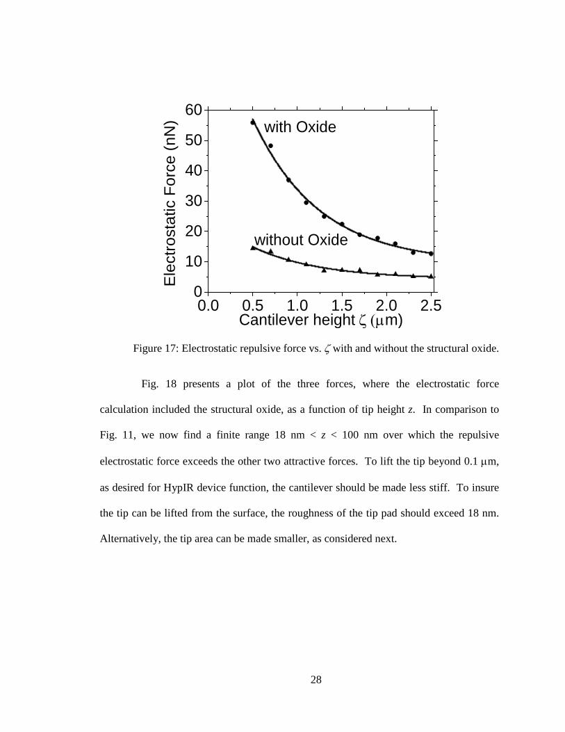
Figure 17: Electrostatic repulsive force vs. ζ with and without the structural oxide.
Fig. 18 presents a plot of the three forces, where the electrostatic force
calculation included the structural oxide, as a function of tip height z. In comparison to
Fig. 11, we now find a finite range 18 nm < z < 100 nm over which the repulsive
electrostatic force exceeds the other two attractive forces. To lift the tip beyond 0.1 µm,
as desired for HypIR device function, the cantilever should be made less stiff. To insure
the tip can be lifted from the surface, the roughness of the tip pad should exceed 18 nm.
Alternatively, the tip area can be made smaller, as considered next.
0.0 0.5 1.0 1.5 2.0 2.50
10
20
30
40
50
60
Ele
ctro
stat
ic F
orce
(nN
)
Cantilever height ζ (µm)
with Oxide
without Oxide
28
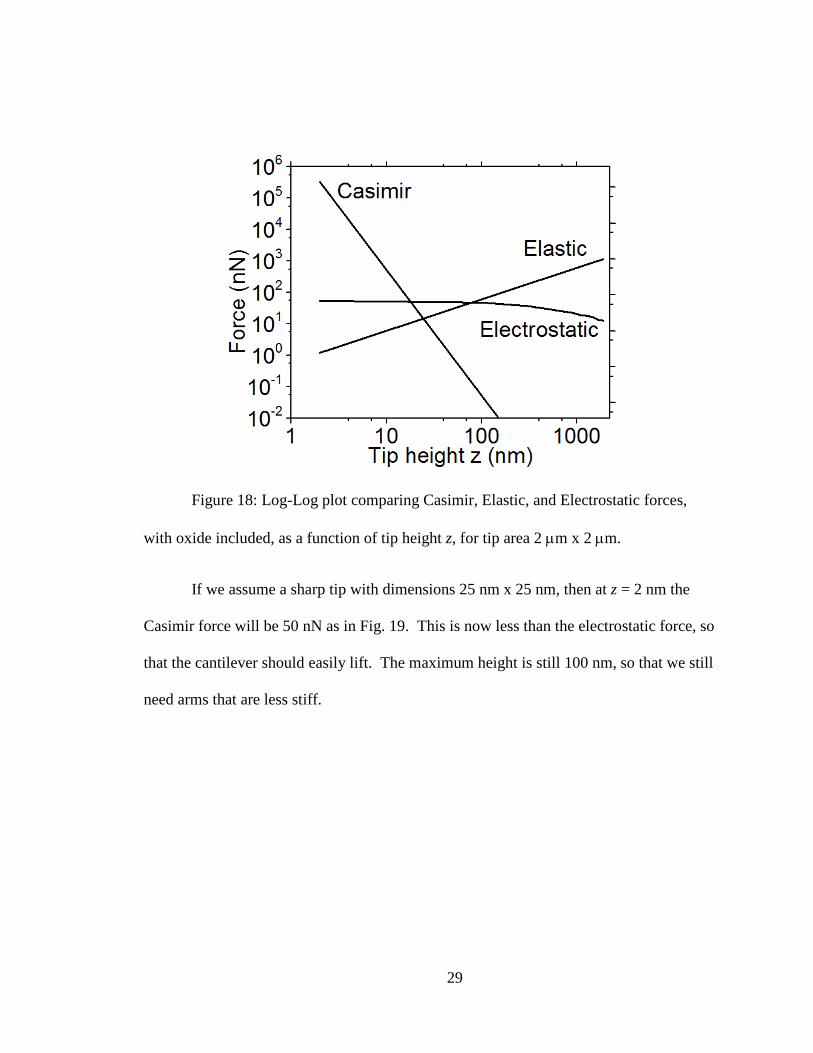
Figure 18: Log-Log plot comparing Casimir, Elastic, and Electrostatic forces,
with oxide included, as a function of tip height z, for tip area 2 µm x 2 µm.
If we assume a sharp tip with dimensions 25 nm x 25 nm, then at z = 2 nm the
Casimir force will be 50 nN as in Fig. 19. This is now less than the electrostatic force, so
that the cantilever should easily lift. The maximum height is still 100 nm, so that we still
need arms that are less stiff.
29
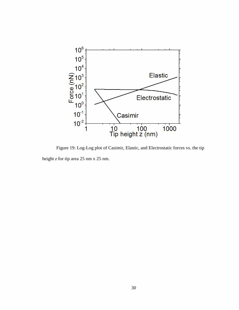
Figure 19: Log-Log plot of Casimir, Elastic, and Electrostatic forces vs. the tip
height z for tip area 25 nm x 25 nm.
30
CHAPTER FIVE: SUMMARY
The Casimir force causes attraction between two metal surfaces at very short
distances of separation. It is considered to be a “contact” force. It is a quantum
electrodynamics phenomenon that arises from zero-point energy of the harmonic
oscillators that are the normal modes of the electromagnetic field. Such “contact” force
creates difficulties in the operation of certain MEMS and NEMS (micro and nano
electromechanical systems) because attractive Casimir force leads to stiction (adhesion)
between the surfaces of MEMS and NEMS devices.
This thesis presented a derivation for the formula for the Casimir force, which
depends strongly on contact area and on separation of the two surfaces. This thesis also
reviews many of the papers that presented studies of the Casimir force studies for
different geometries by experiment and numerical methods. The new science in this
thesis is the evaluation of the Casimir attractive force for single pixel of an infrared
sensor known as “HypIR” that was fabricated by our group at UCF.
HypIR is a MEMS cantilever with a metallic tip that contacts a metallic tip pad.
When an electric bias is applied, the tip is supposed to lift up from the surface by
electrostatic repulsion, but to do so requires that it overcome both the Casimir sticking
force and the elastic restoring force. The three forces were compared theoretically for
geometry as close as practical to that of the actual cantilever that was fabricated.
Calculations were performed with and without considering the permittivity of the
structural oxide, and it was found that the oxide significantly increases the repulsion.
Nevertheless, the results suggest that the cantilever tip should remain stuck to the surface
31

for any electrostatic force available for the allowed range of applied bias, unless the tip
area can be made as small as 25 nm x 25 nm. That the cantilever is observed to lift under
applied bias is a consequence of imperfections in the fabrication that cause the contact
area to be much smaller than anticipated and/or the separation at contact to be
significantly more than the assumed minimum of 2 nm.
32

APPENDIX A: EIGEN FREQUENCIES OF A CUBOIDAL RESONATOR WITH PERFICTLY CONDUCTING WALLS
33
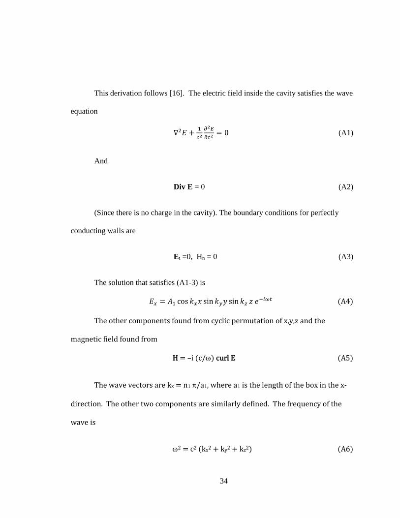
This derivation follows [16]. The electric field inside the cavity satisfies the wave
equation
∇2𝐸𝐸 + 1𝑐𝑐2
𝜕𝜕2𝐸𝐸𝜕𝜕𝑡𝑡2
= 0 (A1)
And
Div E = 0 (A2)
(Since there is no charge in the cavity). The boundary conditions for perfectly
conducting walls are
Et =0, Hn = 0 (A3)
The solution that satisfies (A1-3) is
𝐸𝐸𝑥𝑥 = 𝐴𝐴1 cos 𝑑𝑑𝑥𝑥𝑑𝑑 sin𝑑𝑑𝑦𝑦𝑦𝑦 sin 𝑑𝑑𝑧𝑧 𝑧𝑧 𝑒𝑒−𝑖𝑖𝑖𝑖𝑡𝑡 (A4)
The other components found from cyclic permutation of x,y,z and the
magnetic field found from
H = –i (c/ω) curl E (A5)
The wave vectors are kx = n1 π/a1, where a1 is the length of the box in the x-
direction. The other two components are similarly defined. The frequency of the
wave is
ω2 = c2 (kx2 + ky2 + kz2) (A6)
34

Equation (A2) gives the condition
A1 kx + A2 ky + A3 kz = 0, (A7)
so that only two of the undetermined coefficients A1, A2, A3 are independent.
If none of the n1, n2, n3 are zero, and the coefficients A1, A2 are chosen and
fixed, with A3 determined by Eq. (A7), then there is another set of coefficients A1’ =
A2 ky/kx and A2’ = A1 kx/ky with the same A3 that also satisfies Eq. (A7) with the
same frequency. Thus, each frequency is doubly degenerate in this case.
If one of the n1, n2, n3 is zero, then only one of the components of E is non-
zero. Then there is only one undetermined coefficient, and once this is chosen and
fixed, there are no other modes with the same frequency. Such modes are non-
degenerate.
If two of the n1, n2, n3 are zero, then at least one of the sine terms in each
component of E will be zero, so that E = 0. This means that there are no modes
propagating along any of the cube axes. The lowest frequency is one where one of
the n1, n2, n3 is zero and the other two are 1
35

APPENDIX B: EULER -MACLAURIN FORMULA
36
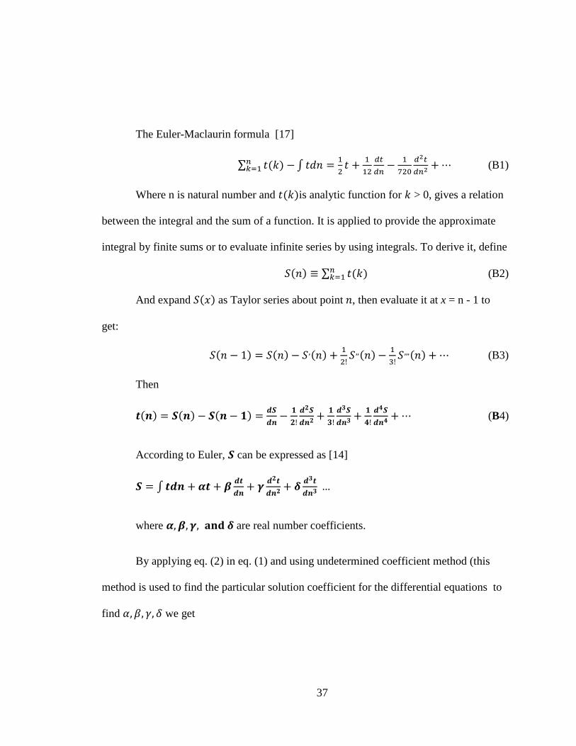
The Euler-Maclaurin formula [17]
∑ 𝑡𝑡(𝑑𝑑) −𝑙𝑙𝑘𝑘=1 ∫ 𝑡𝑡𝑑𝑑𝑑𝑑 = 1
2𝑡𝑡 + 1
12𝑑𝑑𝑡𝑡𝑑𝑑𝑙𝑙− 1
720𝑑𝑑2𝑡𝑡𝑑𝑑𝑙𝑙2
+ ⋯ (B1)
Where n is natural number and 𝑡𝑡(𝑑𝑑)is analytic function for 𝑑𝑑 > 0, gives a relation
between the integral and the sum of a function. It is applied to provide the approximate
integral by finite sums or to evaluate infinite series by using integrals. To derive it, define
𝑆𝑆(𝑑𝑑) ≡ ∑ 𝑡𝑡(𝑑𝑑)𝑙𝑙𝑘𝑘=1 (B2)
And expand 𝑆𝑆(𝑑𝑑) as Taylor series about point 𝑑𝑑, then evaluate it at x = n - 1 to
get:
𝑆𝑆(𝑑𝑑 − 1) = 𝑆𝑆(𝑑𝑑) − 𝑆𝑆 ,(𝑑𝑑) + 12!𝑆𝑆 ,,(𝑑𝑑)− 1
3!𝑆𝑆 ,,,(𝑑𝑑) + ⋯ (B3)
Then
𝒕𝒕(𝒏𝒏) = 𝑺𝑺(𝒏𝒏) − 𝑺𝑺(𝒏𝒏 − 𝟏𝟏) = 𝒅𝒅𝑺𝑺𝒅𝒅𝒏𝒏− 𝟏𝟏
𝟐𝟐!𝒅𝒅𝟐𝟐𝑺𝑺𝒅𝒅𝒏𝒏𝟐𝟐
+ 𝟏𝟏𝟑𝟑!𝒅𝒅𝟑𝟑𝑺𝑺𝒅𝒅𝒏𝒏𝟑𝟑
+ 𝟏𝟏𝟒𝟒!𝒅𝒅𝟒𝟒𝑺𝑺𝒅𝒅𝒏𝒏𝟒𝟒
+ ⋯ (B4)
According to Euler, 𝑺𝑺 can be expressed as [14]
𝑺𝑺 = ∫ 𝒕𝒕𝒅𝒅𝒏𝒏 + 𝜶𝜶𝒕𝒕 + 𝜷𝜷 𝒅𝒅𝒕𝒕𝒅𝒅𝒏𝒏
+ 𝜸𝜸 𝒅𝒅𝟐𝟐𝒕𝒕𝒅𝒅𝒏𝒏𝟐𝟐
+ 𝜹𝜹 𝒅𝒅𝟑𝟑𝒕𝒕𝒅𝒅𝒏𝒏𝟑𝟑
…
where 𝜶𝜶,𝜷𝜷,𝜸𝜸, 𝐚𝐚𝐚𝐚𝐚𝐚 𝜹𝜹 are real number coefficients.
By applying eq. (2) in eq. (1) and using undetermined coefficient method (this
method is used to find the particular solution coefficient for the differential equations to
find 𝛼𝛼,𝛽𝛽, 𝛾𝛾, 𝛿𝛿 we get
37
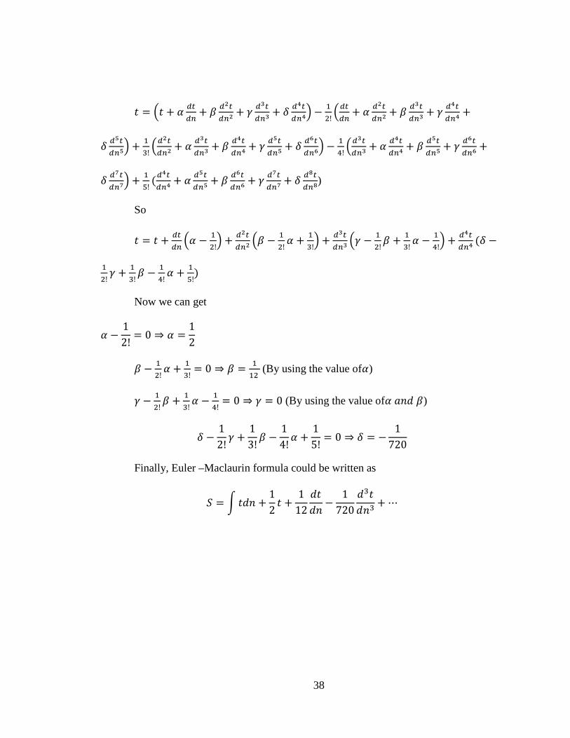
𝑡𝑡 = �𝑡𝑡 + 𝛼𝛼 𝑑𝑑𝑡𝑡𝑑𝑑𝑙𝑙
+ 𝛽𝛽 𝑑𝑑2𝑡𝑡𝑑𝑑𝑙𝑙2
+ 𝛾𝛾 𝑑𝑑3𝑡𝑡𝑑𝑑𝑙𝑙3
+ 𝛿𝛿 𝑑𝑑4𝑡𝑡𝑑𝑑𝑙𝑙4
� − 12!�𝑑𝑑𝑡𝑡𝑑𝑑𝑙𝑙
+ 𝛼𝛼 𝑑𝑑2𝑡𝑡𝑑𝑑𝑙𝑙2
+ 𝛽𝛽 𝑑𝑑3𝑡𝑡𝑑𝑑𝑙𝑙3
+ 𝛾𝛾 𝑑𝑑4𝑡𝑡𝑑𝑑𝑙𝑙4
+
𝛿𝛿 𝑑𝑑5𝑡𝑡𝑑𝑑𝑙𝑙5
� + 13!�𝑑𝑑
2𝑡𝑡𝑑𝑑𝑙𝑙2
+ 𝛼𝛼 𝑑𝑑3𝑡𝑡𝑑𝑑𝑙𝑙3
+ 𝛽𝛽 𝑑𝑑4𝑡𝑡𝑑𝑑𝑙𝑙4
+ 𝛾𝛾 𝑑𝑑5𝑡𝑡𝑑𝑑𝑙𝑙5
+ 𝛿𝛿 𝑑𝑑6𝑡𝑡𝑑𝑑𝑙𝑙6
� − 14!�𝑑𝑑
3𝑡𝑡𝑑𝑑𝑙𝑙3
+ 𝛼𝛼 𝑑𝑑4𝑡𝑡𝑑𝑑𝑙𝑙4
+ 𝛽𝛽 𝑑𝑑5𝑡𝑡𝑑𝑑𝑙𝑙5
+ 𝛾𝛾 𝑑𝑑6𝑡𝑡𝑑𝑑𝑙𝑙6
+
𝛿𝛿 𝑑𝑑7𝑡𝑡𝑑𝑑𝑙𝑙7
� + 15!
(𝑑𝑑4𝑡𝑡
𝑑𝑑𝑙𝑙4+ 𝛼𝛼 𝑑𝑑5𝑡𝑡
𝑑𝑑𝑙𝑙5+ 𝛽𝛽 𝑑𝑑6𝑡𝑡
𝑑𝑑𝑙𝑙6+ 𝛾𝛾 𝑑𝑑7𝑡𝑡
𝑑𝑑𝑙𝑙7+ 𝛿𝛿 𝑑𝑑8𝑡𝑡
𝑑𝑑𝑙𝑙8)
So
𝑡𝑡 = 𝑡𝑡 + 𝑑𝑑𝑡𝑡𝑑𝑑𝑙𝑙�𝛼𝛼 − 1
2!� + 𝑑𝑑2𝑡𝑡
𝑑𝑑𝑙𝑙2�𝛽𝛽 − 1
2!𝛼𝛼 + 1
3!� + 𝑑𝑑3𝑡𝑡
𝑑𝑑𝑙𝑙3�𝛾𝛾 − 1
2!𝛽𝛽 + 1
3!𝛼𝛼 − 1
4!� + 𝑑𝑑4𝑡𝑡
𝑑𝑑𝑙𝑙4(𝛿𝛿 −
12!𝛾𝛾 + 1
3!𝛽𝛽 − 1
4!𝛼𝛼 + 1
5!)
Now we can get
𝛼𝛼 −12!
= 0 ⇒ 𝛼𝛼 =12
𝛽𝛽 − 12!𝛼𝛼 + 1
3!= 0 ⇒ 𝛽𝛽 = 1
12 (By using the value of𝛼𝛼)
𝛾𝛾 − 12!𝛽𝛽 + 1
3!𝛼𝛼 − 1
4!= 0 ⇒ 𝛾𝛾 = 0 (By using the value of𝛼𝛼 𝑎𝑎𝑑𝑑𝑑𝑑 𝛽𝛽)
𝛿𝛿 −12!𝛾𝛾 +
13!𝛽𝛽 −
14!𝛼𝛼 +
15!
= 0 ⇒ 𝛿𝛿 = −1
720
Finally, Euler –Maclaurin formula could be written as
𝑆𝑆 = �𝑡𝑡𝑑𝑑𝑑𝑑 +12𝑡𝑡 +
112
𝑑𝑑𝑡𝑡𝑑𝑑𝑑𝑑
−1
720𝑑𝑑3𝑡𝑡𝑑𝑑𝑑𝑑3
+ ⋯
38

LIST OF REFRENCES
[1] P.W. Milonni and M. Shih, '"Casimir forces," Contemporary Physics, vol. 33, no. 5, pp. 313-322.
[2] S.K. Lamoreaux, '"Demonstration of the Casimir Force in the 0. 6 to 6 μm Range," Phys.Rev.Lett., vol. 78, no. 1, pp. 5-8.
[3] M.J. Madou, '"Fundamentals of microfabrication: the science of miniaturization,", 2002.
[4] L.D. Landau and E.M. Lifshit︠ s︡, '"The classical theory of fields,", vol. 2, Elsevier, 1975.
[5] J.N. Munday, F. Capasso and V.A. Parsegian, '"Measured long-range repulsive Casimir–Lifshitz forces," Nature, vol. 457, no. 7226, pp. 170-173.
[6] E. Lifshitz and L. Pitaevskii, '"Statistical Physics part 2, Landau and Lifshitz course of Theoretical physics,".
[7] M. Sparnaay, '"Attractive forces between flat plates,". Nature, 180, 334-335, 1957.
[8] G. Bressi, G. Carugno, R. Onofrio and G. Ruoso, '"Measurement of the Casimir force between parallel metallic surfaces," Phys.Rev.Lett., vol. 88, no. 4, pp. 041804.
[9] U. Mohideen and A. Roy, '"Precision measurement of the Casimir force from 0.1 to 0.9 μ m," Phys.Rev.Lett., vol. 81, no. 21, pp. 4549.
[10] R.S. Decca and D. LOPez, '"Measurement of the Casimir force using a micromechanical torsional oscillator: electrostatic calibration," International Journal of Modern Physics A, vol. 24, no. 08n09, pp. 1748-1756.
[11] E. Smith, J. Boroumand, I. Rezadad, P. Figueiredo, J. Nath, D. Panjwani, R. Peale and O. Edwards, '"MEMS clocking-cantilever thermal detector,", pp. 87043B-87043B-4.
[12] R. Peale, O. Lopatiuk, J. Cleary, S. Santos, J. Henderson, D. Clark, L. Chernyak, T. Winningham, E. Del Barco and H. Heinrich, '"Propagation and out-coupling of electron-beam excited surface plasmons on gold,".
[13] M. Gedeon, '"Cantilever Beams Part 1 - Beam Stiffnes, no. 20.
[14] I. Rezadad, J. Boroumand, E. Smith, A. Alhasan and R. Peale, '"Repulsive electrostatic froces in MEMS cantilever IR sensors,", vol. 9070, no. 57.
39
[15] "http://www.csc.fi/english/pages/elmer/index_html,".
[16] E. Lifshitz, L. Pitaevskii and L. Landau, "Electrodynamics of Continuous Media: Volume 8," Elsevier, 2008.
[17] R. Roy, '"Sources in the Development of Mathematics,". New York: Cambridge University Press, 2011. Print.
40
Top Related