


Languages
Pages
Legal


Thursday, 14 November, 2013
1
Comparison between POES energetic electron precipitation observations and 1
riometer absorptions; implications for determining true precipitation fluxes 2
Craig J. Rodger 3
Department of Physics, University of Otago, Dunedin, New Zealand 4
Andrew J. Kavanagh and Mark A. Clilverd 5
British Antarctic Survey (NERC), Cambridge, United Kingdom 6
Steve R. Marple 7
Department of Physics, Lancaster University, Lancaster, United Kingdom 8
Abstract. Energetic Electron Precipitation (EEP) impacts the chemistry of the middle 9
atmosphere with growing evidence of coupling to surface temperatures at high latitudes. To 10
better understand this link it is essential to have realistic observations to properly 11
characterise precipitation and which can be incorporated into chemistry-climate models. 12
The Polar-orbiting Operational Environmental Satellites (POES) detectors measure 13
precipitating particles but only integral fluxes and only in a fraction of the bounce loss cone. 14
Ground based riometers respond to precipitation from the whole bounce loss cone; they 15
measure the cosmic radio noise absorption (CNA); a qualitative proxy with scant direct 16
information on the energy-flux of EEP. POES observations should have a direct relationship 17
with ΔCNA and comparing the two will clarify their utility in studies of atmospheric 18
change. We determined ionospheric changes produced by the EEP measured by the POES 19
spacecraft in ~250 overpasses of an imaging riometer in northern Finland. The ΔCNA 20
modeled from the POES data is 10-15 times less than the observed ΔCNA when the 21
>30 keV flux is reported as <106 cm-2sec-1sr-1. Above this level there is relatively good 22
agreement between the space-based and ground-based measurements. The discrepancy 23
occurs mostly during periods of low geomagnetic activity and we contend that weak 24

Thursday, 14 November, 2013
2
diffusion is dominating the pitch angle scattering into the bounce loss cone at these times. A 25
correction to the calculation using measurements of the trapped flux considerably reduces 26
the discrepancy and provides further support to our hypothesis that weak diffusion leads to 27
underestimates of the EEP. 28
29
1. Introduction 30
The coupling of the Van Allen radiation belts to the Earth's atmosphere through 31
precipitating particles is an area of intense scientific interest, principally due to two separate 32
research activities. One of these concerns the physics of the radiation belts, and primarily 33
the evolution of energetic electron fluxes during and after geomagnetic storms [e.g., Reeves 34
et al., 2003] where precipitation losses in to the atmosphere play a major role [Green et al., 35
2004; Millan and Thorne, 2007]. The other focuses on the response of the atmosphere to 36
precipitating particles, with a possible linkage to polar climate variability [e.g., Turunen et 37
al., 2009; Seppalä et al., 2009]. 38
Precipitating charged particles produce odd nitrogen and odd hydrogen in the Earth's 39
atmosphere which can catalytically destroy ozone [Brasseur and Solomon, 2005]. For some 40
time it has been recognized that very intense energetic particle precipitation (EPP) events 41
could lead to significant ozone destruction in the polar middle atmosphere, which was 42
subsequently experimentally observed during solar proton events [e.g., Seppälä et al., 2006; 43
2007]. However, there has also been growing evidence that both geomagnetic storms and 44
substorms produce high levels of energetic electron precipitation [e.g., Rodger et al., 2007; 45
Clilverd et al., 2008, 2012], with modeling suggesting energetic electron precipitation 46
(EEP) can also lead to significant mesospheric chemical changes in the polar regions 47
[Rodger et al., 2010c]. The latter study concluded that the chemical changes could occur 48
with an intensity similar to that of a medium sized solar proton event. In support of this, 49
recent experimental studies have demonstrated the direct production of odd nitrogen 50

Thursday, 14 November, 2013
3
[Newnham et al., 2011] and odd hydrogen [Verronen et al., 2011; Andersson et al., 2012, 51
2013] in the mesosphere by EEP, along with ozone decreases [Daae et al., 2012]. In 52
particular, Andersson et al. [2012] reported experimental evidence of electron precipitation 53
produced odd hydrogen changes stretching over the altitude range from ~52-82 km 54
(corresponding to electrons from ~100 keV to ~3 MeV), while Daae et al. [2012] observed 55
a decrease of 20–70% in the mesospheric ozone immediately following a moderate 56
geomagnetic storm (Kp≈6). 57
There has also been evidence that the effects of energetic particle precipitation may couple 58
into surface climate at high latitudes. Rozanov et al. [2005] and Baumgaertner et al. [2011] 59
imposed a NOx source to represent the EEP-linkage into their chemistry-climate model, and 60
found large (±2 K) variations in polar surface air temperatures. They concluded that the 61
magnitude of the atmospheric response to EEP events could potentially exceed the effects 62
from solar UV fluxes. This conclusion was tested using the experimentally derived ERA-40 63
and ECMWF operational surface level air temperature data sets to examine polar 64
temperature variations during years with different levels of geomagnetic activity [Seppälä et 65
al., 2009]. The latter authors found surface level air temperatures could differ by as much as 66
±4.5 K between high and low geomagnetic storm periods, but that these changes were not 67
linked to changing solar irradiance/EUV-levels. The Seppälä et al. [2009] study argues that 68
the seasonality and temporal offsets observed strongly suggest that the dominant driver for 69
this temperature variability comes from EEP coupling to ozone through NOx production. 70
Very recently additional analysis has shed light on the link between EEP, EPP-generated 71
NOx, and stratospheric dynamics [Seppälä et al., 2013]. This study concluded EEP -72
generated NOx alters planetary wave breaking in the lower stratosphere, leading to more 73
planetary waves propagating into the low latitude upper stratosphere, which then results in 74
the dynamical responses seen later during the winter. 75
Thursday, 14 November, 2013
4
A key component in understanding the link between EEP and atmospheric changes in 76
experimental data are experimental observations of energetic electron precipitation. Further 77
studies making use of chemistry climate models also require realistic EEP observations, or 78
some sort of proxy-representations of EEP in order to characterize the effects. 79
Unfortunately, there are very little experimental observations which can fill this role. The 80
majority of scientific and operational spacecraft measuring energetic electron fluxes in the 81
radiation belts report only the total trapped fluxes, as they do not have sufficient angular 82
resolution to resolve the pitch angles of the Bounce Loss Cone (BLC). This will also be true 83
of the recently launched Van Allen Probes. Scientific studies on energetic electron losses to 84
date have tended to focus on observations from the SAMPEX or Polar-orbiting Operational 85
Environmental Satellites (POES) spacecraft, both of which have significant weaknesses. In 86
the case of SAMPEX the measurements are primarily of the Drift Loss Cone (DLC) rather 87
than the BLC [Dietrich et al., 2010], and are largely limited to an integral electron flux 88
value above ~1 MeV. The Medium Energy Proton and Electron Detector (MEPED) in the 89
Space Environment Monitor-2 (SEM-2) instrument carried onboard POES is unusual in that 90
it includes a telescope which views some fraction of the bounce loss cone [Rodger et al., 91
2010b] but is limited by measuring only 3 integral energy ranges (>30, >100 and 92
>300 keV), while also suffering from significant contamination by low-energy protons 93
[Rodger et al., 2010a]. Recent studies have suggested that the POES EEP measurements 94
may underestimate the true fluxes striking the atmosphere. Comparisons between ground-95
based observations and average MEPED/POES EEP measurements lead to EEP flux 96
magnitudes which differ by factors ranging from 1 to 100, depending on the study [e.g., 97
Clilverd et al., 2012; Hendry et al., 2013; Clilverd et al., 2013]. These studies have 98
suggested that the MEPED/POES electron detectors give a good idea of the variation in 99
precipitation levels, but suffer from large uncertainties in their measurement of flux levels. 100
In contrast, other studies are relying upon MEPED/POES precipitation measurements to 101

Thursday, 14 November, 2013
5
feed chemistry-climate models. One example of this is the Atmospheric Ionization Module 102
OSnabrück (AIMOS) model which combines experimental observations from low-Earth 103
orbiting POES spacecraft along with geostationary measurements and with geomagnetic 104
observations to provide 3-D numerical model of atmospheric ionization [Wissing and 105
Kallenrode, 2009]. AIMOS-outputs during SPE and geomagnetic storms have been used to 106
draw conclusions as to the relative significance of such events to the middle atmosphere 107
[e.g., Funke et al., 2011], and a validation of AIMOS-outputs for altitudes >100 km altitude 108
has been undertaken [Wissing et al., 2011]. 109
In order to make best use of MEPED/POES EEP measurements it is necessary to better 110
understand these measurements and how they compare with experimental observations of 111
the impact of the EEP upon the middle atmosphere and lower ionosphere. In this paper we 112
examine MEPED/POES EEP measurements during satellite overflights of a riometer 113
located in Kilpisjärvi, Finland. As the riometer responds to EEP by measuring the 114
ionospheric changes produced by the EEP, there should be a direct relationship between the 115
EEP observations and the riometer absorption changes. We use modeling to link the two, 116
fitting the integral flux channels with a power-law and determining the change in electron 117
density profile that would then arise in the lower ionosphere. A direct comparison can then 118
be made between the riometer response predicted by the satellite EEP observations and the 119
experimentally observed riometer absorptions. Our goal in this study is to test the accuracy 120
of the MEPED/POES satellite EEP measurements, as well as providing better understanding 121
of the mechanisms driving EEP. 122
2. Data Descriptions 123
2.1 POES Satellite SEM-2 Data 124
The second generation Space Environment Module (SEM-2) [Evans and Greer, 2004] is 125
flown on the Polar Orbiting Environmental Satellites (POES) series of satellites, and on the 126

Thursday, 14 November, 2013
6
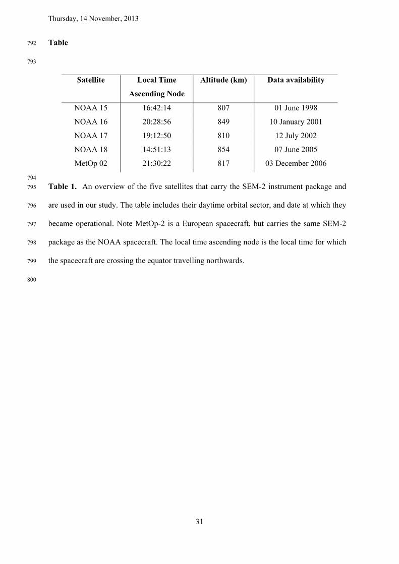
Meteorological Operational (MetOp)-02 spacecraft. Table 1 contains a summary of the 127
SEM-2 carrying spacecraft operational during our study period, which spans from mid-1998 128
when NOAA-15 starts to provide scientific observations through to the end of 2008. These 129
spacecraft are in Sun-synchronous polar orbits with typical parameters of ~800−850 km 130
altitude, 102 min orbital period and 98.7° inclination [Robel, 2009]. The orbits typically are 131
either morning or afternoon daytime equator crossings, with corresponding night-time 132
crossings. 133
In this study we use SEM-2 Medium Energy Proton and Electron Detector (MEPED) 134
observations. The SEM-2 detectors include integral electron telescopes with energies of 135
>30 keV (e1), >100 keV (e2), and >300 keV (e3), pointed in two directions. In this study we 136
focus primarily upon the 0º-pointing detectors. The telescopes are ±15º wide. Modeling work 137
has established that the 0° telescope monitor particles in the atmospheric bounce loss cone 138
that will enter the Earth's atmosphere below the satellite when the spacecraft is poleward of 139
L≈1.5-1.6, while the 90° telescope monitors trapped fluxes or those in the drift loss cone, 140
depending primarily upon the L-shell [Rodger et al., Appendix A, 2010b]. 141
Rodger et al. [2010a] found that as much as ~42% of the 0° telescope >30 keV electron 142
observations from MEPED were contaminated by protons in the energy range ~100 keV-143
3 MeV [Yando et al., 2011] although the situation was less marked for the 90° telescope 144
(3.5%). However, NOAA has developed new techniques to remove this proton contamination 145
as described in Appendix A of Lam et al. [2010]. This algorithm is available for download 146
through the Virtual Radiation Belt Observatory (ViRBO; http://virbo.org), and has been 147
applied to all of the data in our study. This algorithm does not work for solar proton events as 148
we will discuss later. 149
150
2.2 Viewing the Bounce Loss Cone 151
Thursday, 14 November, 2013
7
Before discussing the criteria for data selection we briefly summarize some relevant features 152
concerning pitch angles in the radiation belts; more detailed descriptions may be found 153
elsewhere [e.g., Walt, 1984; Spjeldvik and Rothwell, 1985]. The pitch angle (α) of a charged 154
particle in the radiation belts is defined by the angle between the particle velocity vector and 155
the magnetic field line. While the pitch angle changes along the magnetic field line, a locally 156
trapped particle has a pitch angle of 90º. Particles trapped in the radiation belts have a range 157
of pitch angle at the geomagnetic equator from 90º down to the bounce loss cone angle, 158
(αBLC), and pitch angles are generally referenced to the geomagnetic equator. Any particle 159
whose pitch is smaller than αBLC will mirror at altitudes below ~100 km, inside the Earth's 160
atmosphere, and thus have a high probability of encountering an atmospheric molecule and 161
being lost through precipitation. In practice, a particle whose pitch angle lies inside the BLC 162
will precipitate out within a small number of bounces. 163
The angular width of the BLC is dependent on the geomagnetic field strength at ~100 km, 164
which varies across the Earth. Thus αBLC will vary locally as the particle drifts around the 165
Earth (eastwards for electrons and westwards for protons). A radiation belt particle will 166
experience the lowest field strengths, and thus the largest local αBLC, around the Antarctic 167
Peninsula and Weddell Sea (for the inner radiation belt), and south of the Antarctic Peninsula 168
(for the outer radiation belt). The local BLC with the largest angular width establishes the 169
Drift Loss Cone (DLC), which has angular width of αDLC in pitch angle space. Figure 1 shows 170
a schematic of the loss cones in pitch angle space, including an electron which has a pitch 171
angle located outside of the DLC, and thus will be mirroring above the atmosphere. A particle 172
with a pitch angle lying between αDLC and αBLC (i.e., αBLC<α<αDLC) will drift around the world 173
mirroring just above the atmosphere until reaching the same longitudes as the South 174
American Magnetic Anomaly (SAMA), at which point the local αBLC grows until αBLC>α and 175
the particle precipitates. Examples of this can be seen in the scattering of inner belt electrons 176
into the DLC by a ground-based VLF transmitter [e.g., Gamble et al., Fig. 5, 2008; Rodger et 177
Thursday, 14 November, 2013
8
al., Fig. 6, 2010b]. Recent evidence has been put forward showing that there is increased 178
atmospheric HOx concentrations for the locations where the particles in the DLC precipitate 179
into the atmosphere [Andersson et al., 2013]. To fully characterize the loss of radiation belts 180
electrons into the atmosphere would require an instrument capable of unambiguously 181
resolving the BLC and thereby determining the full flux of precipitating electrons. Such a 182
measurement is not currently available, the best we have is the 0º MEPED telescope, but this 183
data clearly have limitations as we will explore. 184
For the vast majority of locations relevant to precipitation from the radiation belts, 185
substorms or solar proton events, the 0º MEPED telescope only views particles with pitch 186
angles inside the BLC [Rodger et al., Fig A3, 2010b]. However, at POES-altitudes αBLC is 187
significantly larger than the ±15º telescope width, such that the 0° telescope only observes a 188
fraction of the bounce loss cone. Figure 2 provides an estimate of how this varies across the 189
globe, building on the Rodger et al. [Appendix A, 2010b] modeling. For large portions of the 190
Earth only 40-50% of the BLC radius is viewed, decreasing to zero near the geomagnetic 191
equator where the 0° telescope would view locally trapped particles (should such a population 192
exist). The fraction of the BLC viewed by the 0° telescope is shown for two specific locations 193
in Figure 3. This shows the situation for the magnetic field line which starts 100 km in 194
altitude above the Kilpisjärvi riometer facility (69.05ºN, 20.79 ºE, IGRF L=6.13; left hand 195
panel) and for comparison the Antarctic station Halley (75.5ºS, -26.9 ºE, IGRF L=4.3; right 196
hand panel). In this plot the centered cross represents the magnetic field line, while the dotted 197
black line shows the viewing window the ±15º-wide 0° MEPED electron telescope, 198
transformed to the geomagnetic equator. The equatorial pitch angle for the centre of the 0° 199
telescope is shown by a circled cross. The angular size of the BLC is shown by the heavy 200
black line, while the angular size of the DLC is shown by the light grey line. Note that for 201
Kilpisjärvi the DLC is essentially the same size as the BLC, and hence is not visible. In the 202
case of Kilpisjärvi, the 0° MEPED electron telescope will sample 52% of the radial pitch 203
Thursday, 14 November, 2013
9
angle range, and ~7% of the BLC area, while for the contrasting case of Halley, the telescope 204
samples 57% of the radial range and ~7.5% of the BLC area. 205
Basic radiation belt physics suggests that the fluxes in the BLC will exhibit circular 206
symmetry and that the flux in the BLC may not be constant with pitch angle; one would often 207
expect considerably more flux near the αBLC rather than near the centre of the loss cone. In the 208
common case where pitch angle scattering involves smaller changes towards αBLC, described 209
as "weak diffusion", there are likely to be large differences between the edge and centre of the 210
BLC. Therefore the 0º telescope (as seen in Figure 2) could be failing to view a considerable 211
amount of the flux in the BLC and in this study we seek to test the importance of this issue. In 212
practice MEPED/POES electron telescope observations are converted from counts to flux 213
through a geometric conversion factor [Evans and Greer, 2004; Yando et al., 2011] which 214
takes into account the angular size of the telescope, as well as its sensitivity. This converts the 215
counts measured by the telescope into an isotropic flux fully filling the BLC. 216
217
2.3 Contamination by high proton fluxes 218
During solar proton events large fluxes of high energy protons (>5 MeV) gain direct access 219
to the geomagnetic field; the NOAA correction algorithm does not work at these times 220
resulting in the appearance of large unphysical electron fluxes deep in the polar cap. We 221
therefore remove all measurements at times when the MEPED P7 omni-directional 222
observations of >36 MeV protons reports >3 counts/s. We find this adequately removes the 223
contamination caused by SPE. Figure 4 shows examples of the typical (median) >100 keV 224
precipitating flux maps for the time period 1 January 2004- 31 December 2008. The upper 225
panels are for quiet and moderately disturbed geomagnetic conditions (taken as when Kp≤5-), 226
while the lower panels are for geomagnetic storm conditions (taken as when Kp>5-). In this 227
figure the left hand panels show the median fluxes when the P7 threshold is not applied, while 228
the right hand panels are after the threshold. The very large values above the SAMA are 229
Thursday, 14 November, 2013
10
totally removed, indicating the extremely large precipitating electron fluxes reported in this 230
region are unreal and most likely caused by inner belt protons. Further support for this has 231
recently been put forward from atmospheric HOx observations [Andersson et al., 2013]. 232
While the footprint of the outer radiation belt was visible in the atmospheric HOx 233
concentrations (and in particular the signature of the DLC), there was no HOx signature in the 234
SAMA, confirming both that the 0º fluxes are incorrect in that region and also that there is 235
very low precipitation. 236
During quiet geomagnetic conditions (upper panels of Figure 4) precipitation can occur from 237
the outer radiation belts in any longitude. However, it is enhanced in the longitudes of the 238
Antarctic Peninsula and south of Africa, where electrons in the DLC precipitate into the 239
atmosphere. This signature is not seen for geomagnetic storm conditions (lower panels of 240
Figure 4), where all longitudes experience essentially the same precipitation from the 241
radiation belts. Similar results were reported earlier by Horne et al. [2009], who showed a 242
similar map for >300 keV precipitating electrons during the main phase of storms. That study 243
argued that the storm time behavior of these electrons indicated "strong diffusion" [Kennel 244
and Petschek, 1966; Baker et al., 1979] was taking place, where pitch angle scattering is 245
strong enough to scatter electrons into the bounce loss cone and cause precipitation at any 246
longitude. In contrast, the upper panels are more consistent with weak diffusion occurring, 247
where the electrons are mainly scattered into the drift loss cone and drift around the Earth to 248
the longitudes of the Antarctic Peninsula where they are lost to the atmosphere. 249
250
2.4 Kilpisjärvi Riometer data 251
We will compare the 0° telescope electron observations with riometer absorption 252
observations from the IRIS (Imaging Riometer for Ionospheric Studies) instrument in 253
Kilpisjärvi, Finland (69.05ºN, 20.79ºE, IGRF L=6.13, Figure 5) [Browne et al., 1995]. 254
Riometers (relative ionospheric opacity meter) utilize the absorption of cosmic radio noise by 255
Thursday, 14 November, 2013
11
the ionosphere [Little and Leinbach, 1959] to measure the enhancement of D-region electron 256
concentration caused by EEP. The riometer technique compares the strength of the cosmic 257
radio noise signal received on the ground to the normal sidereal variation referred to as the 258
absorption quiet-day curve (QDC) to produce the change in cosmic noise absorption (ΔCNA) 259
above the background level. The cosmic radio noise propagates through the ionosphere and 260
part of the energy is absorbed due to the collision of the free ionospheric electrons with 261
neutral atmospheric atoms. 262
The Kilpisjärvi IRIS is a 64-antenna, 49 beam configuration [Detrick and Rosenberg, 1990], 263
that records the X-mode cosmic radio noise at 38.2 MHz. The central beam (labeled as beam 264
25) of the array has a width of 11.17°; the beam-width increases to a maximum of 13.89° for 265
beams at the edge of the array and the wide beam has a width of ~90°. The field of view 266
encompasses 5° (3°) longitude and 2° (1.5°) latitude in geographic (geomagnetic) coordinates. 267
All of the beams are sampled every second, recording the cosmic radio noise at 38.2 MHz. 268
QDC for IRIS are derived from the data using an advanced variant of the percentile method 269
described in Browne et al. [1995]. At least 16 days of contiguous data (covering the desired 270
period of observation and enough days to ensure a quiet period) are smoothed using a median 271
filter (of length 599 seconds). The data are then binned according to sidereal time and sorted 272
in descending order. Next the mean of the m-th to n-th highest values are taken: for 273
geomagnetically quiet times, when there are many quiet days, typical values are m = 4 and n 274
= 5; for more active periods, with fewer quiet days, typical values are m = 2 and n = 3. These 275
mean values provide the basis for the QDC, which is further smoothed with a truncated 276
Fourier series and filtered via Fourier transform to remove high frequency components. 277
Deriving the QDC in this manner removes CNA from solar ionization (such that ΔCNA is 278
references to ‘zero’ for IRIS) and limits system specific effects (such as antenna deterioration 279
and snow accumulation at the site). Filtering techniques are applied to the data prior to QDC 280
formation to remove the effects of solar radio emission and scintillation from radio stars. The 281

Thursday, 14 November, 2013
12
former can lead to underestimates of the ΔCNA since the received power is boosted above the 282
level we would expect from the radio sky [Kavanagh et al., 2004b] when the Sun is in the 283
beam or a major side-lobe of the riometer. The QDC will always have some small uncertainty 284
in how well they represent the ‘zero’ line, but all curves for this study have been visually 285
inspected. It is the availability of this long dataset of carefully checked ΔCNA observations 286
which caused us to focus upon the Kilpisjärvi IRIS for the current study, rather than other 287
similar systems located around the world. 288
The resultant ΔCNA is primarily a measure of EEP, being sensitive to electron number 289
density changes in the D-layer of the ionosphere. There have been attempts to link ΔCNA to 290
fluxes of electrons using simple models [e.g. Collis et al., 1984] and some success at using 291
overlapping imaging riometers to determine the height of the absorbing layer and hence the 292
responsible energy [e.g. Wild et al., 2010]. The riometer has the potential to be an important 293
ground truth for satellite studies since it is sensitive to all of the precipitating electrons with 294
energy >30 keV. 295
3. Data Selection 296
IRIS data have been recorded continuously since September 1994 at 1 second cadence (in 297
practice limited data gaps occur due to technical faults at the riometer site). In this study we 298
use 1 minute means around the time the satellite passes the L-shell of the riometer but only 299
use a ‘minute’ interval if there are at least 20 seconds of valid observations within the minute 300
of the satellite pass. If the absorption is negative we assume the QDC is not well fitted and 301
discard the data. The magenta star in Figure 5 shows the location of the riometer. As the EEP 302
will follow the field line until striking the atmosphere, we do not take POES observations 303
directly above the riometer. The red cross in Figure 5 shows the subsatellite location for a 304
fieldline at POES-altitudes which is traced down the geomagnetic field to the atmosphere 305
above Kilpisjärvi using IGRF. Conjunctions between IRIS and POES are identified as when 306

Thursday, 14 November, 2013
13
the satellite passes within ±3º in latitude and ±10º in longitude of the Kilpisjärvi riometer 307
(taking into account the need to correct for field-line tracing). As an extreme limit, we require 308
at least two 1 s MEPED/POES observations in a single overpass to include data from that 309
overpass and typically there are between ten and eleven 1-s samples included in each 310
overpass. 311
For this study we use the three precipitating electron channels of MEPED/POES (e1, e2, and 312
e3 channels) fitted to a power-law using least squares fitting and we require that the fitted 313
power law is within ±50% of the observed >30 keV precipitating electron flux for the fit to be 314
regarded as valid. A further constraint is the noise floor of the MEPED/POES electron 315
observations, which is a flux of 100 electrons cm-2s-1sr-1; consequently we remove any passes 316
where this constraint is breached. 317
A riometer is sensitive to any process that changes the electron number density in the lower 318
ionosphere such as solar proton precipitation or X-ray impact from solar flares. The latter are 319
excluded by limiting observations to night-side periods where the solar zenith angle >120º. 320
This also removes contamination of the riometer signal by solar radio emission; Kavanagh et 321
al. [2004] showed that radio bursts can lead to underestimates of CNA and in the most severe 322
cases will produce negative ΔCNA values by increasing the received signal above the natural 323
QDC level. Characterizing and correcting for this problem is not a simple process [Kavanagh 324
et al., 2012]. We remove the effect of solar proton events using the 8.7- 14.5 MeV proton 325
observations from GOES; when the flux in this energy range is ≥0.75 counts cm-2s-1sr-1MeV-1 326
we exclude that time period. As stated earlier the MEPED/POES instrument detects protons 327
[e.g., Neal et al., 2013]; however it is less sensitive than those made by GOES such that small 328
events which are observable in ground-based ionospheric data [Clilverd et al., 2006] are not 329
visible in MEPED/POES data and also do not meet the "standard definition" of a solar proton 330
event determined using GOES data as they are too "weak". 331

Thursday, 14 November, 2013
14
From the original Kilpisjärvi 1-minute dataset spanning 1995-2008, 27.5% of the data is 332
removed from the data quality tests, and an additional 3% by the POES proton thresholding. 333
The requirement that the ionosphere above Kilpisjärvi is not Sun-lit is considerably more 334
prescriptive, and after this is enforced 92.6% of the data has been removed, leaving 7.4% of 335
the total dataset which is of good quality, unaffected by solar protons and for a nighttime 336
ionosphere. This is equal to 380.0 days of 1-minute observations (547,255 samples). By 337
observing the additional criteria outlined above, and in particular the requirement for a 338
spatially close overpass, we are left with a maximum of 254 conjunctions between 1 June 339
1998 and 31 December 2008, with acceptable data from both MEPED/POES and IRIS. Due 340
to the listed constraints there are 254 median EEP values and 243 mean EEP values that can 341
be used for comparison. 342
4. Modeling of electron-density produced ionization changes 343
4.1 EEP produced changes in electron number density 344
In order to estimate the response of the riometer data to EEP, we follow the calculation 345
approach outlined by Rodger et al. [2012]. This approach allows one to use POES EEP 346
observations to determine riometer absorption, by determining the changing ionospheric 347
electron number density and hence calculating the changing radio wave absorption. We 348
determine the change in ionospheric electron number density over the altitude range 40-349
150 km caused by precipitation assuming EEP spanning the energy range 10 keV-3 MeV. 350
The ambient, or undisturbed electron density profile, is provided by the International 351
Reference Ionosphere (IRI-2007) [online from 352
http://omniweb.gsfc.nasa.gov/vitmo/iri_vitmo.html] for 16 January at 23.5 UT for night 353
conditions, with the "STORM" model switched off. As the IRI does not include all of the D-354
region, particularly during the nighttime, we combine the IRI results with typical D-region 355
electron density profiles determined for nighttime conditions [Thomson and McRae, 2009]. 356

Thursday, 14 November, 2013
15
Riometer ΔCNA values for the X-mode are calculated from the EEP flux after determining 357
the electron number density profile as outlined in section 2.4 of Rodger et al. [2012], after 358
which riometers absorption values are calculated following the equations in section 2.1 of 359
Rodger et al. [2012]. 360
The MEPED/POES electron precipitation observations are of integral fluxes, which must 361
be transformed into differential fluxes in order to determine ionisation rates and hence the 362
ionospheric changes. As a starting point, we consider the case of EEP with an energy 363
spectrum provided by experimental measurements from the DEMETER spacecraft [Clilverd 364
et al., 2010], which were found to be consistent with a power law relationship. A more 365
general examination of DEMETER electron observations also concluded that power-laws 366
were accurate representations of the flux spectrum [Whittaker et al., 2013]. While 367
DEMETER primarily measured electrons in the DLC, its measurements are more likely to 368
be representative of the BLC than those of the trapped electron fluxes. 369
370
4.2 Case Study 371
Before examining the larger dataset of over-passes, we start by presenting a case-study 372
where a single POES spacecraft passes very close to the Kilpisjärvi riometer. On 3 373
December 2005 at 01:54 UT the NOAA-18 satellite passed within ~0.3º of the Kilpisjärvi 374
riometer (taking into account the need to correct for fieldline tracing). At this time the AE 375
index was 442 nT, suggesting a period of substorm activity. This is also consistent with the 376
riometer vertical beam ΔCNA, which recorded 1.13 dB ± 0.09 dB and the mean/median 377
value of the Kilpisjärvi riometer array (excluding the corner beams) was 378
0.9503 dB/0.9151 dB, respectively. We accept MEPED/POES electron precipitation 379
observations from NOAA-18 when it is within ±3º latitude of Kilpisjärvi, leading to twelve 380
1-s samples spanning 24 s. The EEP observations are high, also consistent with substorm 381
activity. The mean >30, >100 and >300 keV precipitating fluxes reported were 3.54×10⁶, 382

Thursday, 14 November, 2013
16
2.61×10⁴, and 514.3 electrons cm-2s-1sr-1, while the median fluxes are 3.69×10⁶, 2.02×10⁴, 383
and 514.3 electrons cm-2s-1sr-1. Note that the median and mean are very similar to one 384
another (the >30 keV values differ by only ~4%). Following the process outlined in Section 385
4.1 we use these EEP observations to determine the changed ionospheric electron density 386
profile and hence calculate a predicted ΔCNA. These are 1.09 dB for the mean EEP 387
observations and 1.13 dB for the median EEP observations, thus highly consistent with the 388
experimental riometer observations. 389
This suggests that it is possible to directly relate POES EEP fluxes with riometer 390
absorption measurements. In the following sections we investigate this further, and for a 391
wider range of geomagnetic conditions. 392
393
4.3 All POES overflights 394
We now expand our analysis to calculate predicted ΔCNA values for all of the over-flights 395
identified in section 3; these are shown in the left hand panel of Figure 6. The ΔCNA 396
calculations for both mean (green stars) and median (red stars) EEP fluxes are shown, along 397
with the experimentally observed ΔCNA from the IRIS vertical riometer beam (blue 398
squares). In this figure we also show polynomial fits (3rd order) between the observed 399
>30 keV EEP fluxes and the various ΔCNA. In general, the ΔCNA calculated from the 400
mean and median EEP fluxes are the same, with the green (mean) and red (median) fitting 401
lines lying almost on top of one another. Uncertainties in the experimental data are 402
calculated from the standard error using the observed variance of the ΔCNA in each minute. 403
The dashed blue lines in the left hand panel shows fitted lines to the experimentally 404
observation uncertainty range. There is considerably more scatter in the experimentally 405
observed ΔCNA, although there is a clear tendency for experimental riometer observations 406
to show higher ΔCNA for larger EEP fluxes, as expected. At low EEP fluxes there is an 407
offset between the observed and calculated ΔCNA, with the calculated values being ~7-9 408

Thursday, 14 November, 2013
17
times lower than experimentally observed. This is not the case for high EEP fluxes, where 409
there is much better agreement, and no clear evidence of a consistent offset. 410
For a given satellite-observed >30 keV EEP flux there is considerable scatter in the 411
experimentally observed ΔCNA. Some of this scatter will be due to experimental 412
uncertainty, as reflected by the dashed lines in Figure 6, e caused by spatial and temporal 413
variations between the EEP observed by the satellite at its location, and that striking the 414
ionosphere above the riometer. Analysis of a subset of riometer absorption events suggests 415
that temporal variations over ~30 s timescales can account for the majority of the scatter 416
observed in the experimental observations. The scatter in the calculated ΔCNA is caused by 417
the different energy spectra determined for each event from the satellite data. While there is 418
significantly more scatter in the experimental observations, there is clearly an offset 419
between the experimental and calculated ΔCNA values. 420
One possible explanation for the differences between the observed and calculated riometer 421
absorptions is fine structure in the EEP, such that the vertical-directed beam is not a good 422
representation of the typical absorption occurring across a wide field of view. In the right 423
hand panel of Figure 6 we also plot the mean ΔCNA from across the entire Kilpisjärvi IRIS 424
array, excluding the four corner beams (beams 1, 7, 43, 49). Again, a polynomial best fit 425
line is included, suggesting that typically the vertical beam is a good estimate of the average 426
ΔCNA expected for a wide-beam case. Essentially the same consistent offsets are seen in 427
the right-hand and left-hand panels of Figure 6. It is also not possible to explain the offsets 428
in terms of the longitudinal distance between the spacecraft overflight and the location of 429
Kilpisjärvi, as the calculated ΔCNA are consistently high for low fluxes independent of this 430
distance (not shown). 431
432
4.4 Sensitivity to Electron Energy Spectrum 433

Thursday, 14 November, 2013
18
In the analysis above we assumed that the EEP was described by a power-law spectral 434
gradient, following the evidence in the experimental literature. The form of the calculated 435
ΔCNA in Figure 6 is quite strongly linked to the power-law fitted to the POES-observed 436
EEP fluxes. For low ΔCNA values, associated with >30 keV fluxes less than 103 cm-2s-1sr-1, 437
the spectrum is very "flat" with power-laws larger than -1.5. This is to be expected as the 3 438
flux measurements are close to the 102 cm-2s-1sr-1 noise floor value for all channels. With 439
increasing flux magnitude the power-law spectral gradient becomes increasingly negative, 440
with values of -4 to -5 at the highest magnitudes. 441
In order to test the sensitivity of the calculations shown in Figure 6, and in particular the 442
offset observed, we consider some different representations for the EEP. We undertook the 443
same analysis as described above, but used an e-folding relationship to describe the energy 444
spectrum. This produces (not shown) fewer valid fits (167 rather than 243) but essentially 445
the same fitted lines seen in the left-hand panel of Figure 6 (i.e., the green and blue lines). 446
5. Difference between calculated and Observed ΔCNA 447
5.1 Spatial variability of precipitation 448
We have already considered that differences between the observed ΔCNA and that 449
calculated from the MEPED/POES EEP fluxes might be due to local fine structure and 450
established that this cannot explain the offsets. The overpass criterion is that POES must fly 451
within ±3º in latitude and ±10º in longitude of the central location of IRIS. The IRIS field of 452
view encompasses 2º latitude and 5º longitude and consequently there will be times when 453
the over flights are not directly within the fields of view. It is established that ΔCNA can 454
display large variations in precipitation across several degrees of longitude; this can stem 455
from the variability of the substorm injection region location on the night side [e.g. 456
Kavanagh et al., 2007], the presence of discrete, but moderately energetic forms such as 457
omega bands [Kavanagh et al., 2009] or from the presence of geomagnetic pulsations 458
Thursday, 14 November, 2013
19
modulating the precipitation [e.g. Beharrel et al., 2010]. We have tested whether the 459
longitudinal separation can explain the observed offsets, but there is no relationship 460
between the two: the calculated ΔCNA are consistently high for low fluxes independent of 461
the longitudinal separation (not shown). 462
463
5.2 Dependence upon Geomagnetic Activity 464
Figure 4 showed that the EEP flux magnitude had a strong dependence upon geomagnetic 465
storm levels, consistent with multiple previous studies [e.g., Clilverd et al., 2010, Whittaker 466
et al., 2013]. The upper panels of Figure 7 show the dependence of calculated (left hand 467
panel) and observed (upper right hand panel) ΔCNA on geomagnetic activity, in this case 468
through Kp. Both the calculated ΔCNA (taken from POES EEP observations) and the 469
observed ΔCNA show a general organization depending on Kp; very small ΔCNA occur at 470
geomagnetically very quiet times (Kp<2), while larger ΔCNA occur during more disturbed 471
conditions. There is not a one-to-one relationship between the ΔCNA and Kp, which may 472
indicate that the EEP flux-levels vary strongly on short time scales (i.e., from minute to 473
minute) when contrasted with the 3-hour resolution of the Kp parameter. Nonetheless, there 474
is a broad organization of the ΔCNA with Kp (and to a weaker extent, AE (not shown). This 475
is somewhat consistent with previous studies [e.g. Kavanagh et al., 2004a] that have shown 476
an organization with Kp but with a large spread of absorption values. 477
478
5.3 Dependence upon Weak/Strong Diffusion 479
Figure 6 suggests that there is a significant disagreement between the POES-predicted 480
ΔCNA and that observed, but only for smaller EEP fluxes, less than about 105-106 cm-2s-1sr-481
1 for >30 keV electrons. This issue is very likely to occur during quiet geomagnetic 482
conditions or weaker geomagnetic disturbances (as seen in the upper panels of Figure 7). 483
One possible reason for the POES-predicted ΔCNA being lower than that observed is 484
simply that the MEPED/POES 0º-directed telescope fails to measure the EEP occurring in 485

Thursday, 14 November, 2013
20
these cases. As noted in Section 2.2, EEP may occur for pitch angles near the edges of the 486
BLC, but be missed by the 0º-directed telescope. This is more likely when weak diffusion is 487
occurring, that is when the pitch angle scattering processes involve small changes in pitch 488
angle and the peak fluxes are close to the edge of the BLC. Our suggestion is consistent for 489
quiet and weakly disturbed geomagnetic conditions when weak diffusion is expected to be 490
more observable. During strong disturbances we expect strong diffusion to dominate. We 491
consider that weak diffusion could be a factor in the observed offsets during these periods 492
of low geomagnetic activity. We test this idea in the lower panels of Figure 7, which show 493
the mean EEP >30 keV fluxes reported over Kilpisjärvi in the 0º- and 90º-directed 494
telescopes. The 90º telescope largely observes electrons which are stably trapped [Rodger et 495
al., 2010b], but are mirroring at POES satellite altitudes, and thus have equatorial pitch 496
angles which are not much above the DLC or BLC angles. During weak diffusion pitch 497
angle scattering one would expect large differences between the fluxes of the 0º and 90º 498
telescopes. However, during strong diffusion electrons will be pitch angle scattered from 499
high pitch angles towards the BLC, and will pass through the pitch angle range of the 90º 500
telescope on the way to the pitch angle range of the 0º telescope (and hence being lost). 501
While the pitch angles measured by the 90º telescope are trapped fluxes, for strong diffusion 502
processes those electrons rapidly move to lower pitch angles and thus precipitate into the 503
atmosphere. 504
We use colored dots in the lower panels of Figure 7 to show the riometer ΔCNA and how 505
it relates to the MEPED/POES observed fluxes. The lower left hand panel shows the ΔCNA 506
calculated from mean EEP fluxes while the lower right hand panel shows the observed 507
ΔCNA at Kilpisjärvi. When the EEP fluxes are low and the ΔCNA is are small, there is ~2 508
orders of magnitude difference between the 0º telescope and 90º telescope fluxes, consistent 509
with weak diffusion. In contrast, when the ΔCNA is large (~0.5-0.6 dB) the 90º telescope 510
fluxes are only 20-50% larger than those reported by the 0º telescope, suggesting strong 511

Thursday, 14 November, 2013
21
diffusion is taking place. This would appear to explain why the POES-predicted ΔCNA are 512
in reasonable agreement with observations for high EEP fluxes, as the BLC will be full and 513
the pitch angle range viewed by the 0º telescope will provide a good approximation for the 514
BLC fluxes. 515
We now test the extent to which the MEPED/POES observed fluxes underestimate the 516
"true flux" in the BLC. The left hand panel of Figure 8 shows the polynomial fits for the 517
observed ΔCNA at Kilpisjärvi (blue line), and that calculated from the Mean and Median 518
POES EEP fluxes (green and red lines, respectively), taken from Figure 6. The black lines 519
in this figure show the ΔCNA calculated from the Mean POES EEP fluxes boosted by 3, 10 520
and 30 times. For POES >30 keV EEP fluxes below 104 cm-2s-1sr-1, the satellite-reported 521
fluxes need to be increased by ~10-15 times in order to reproduce the observed ΔCNA. For 522
satellite fluxes ~105 cm-2s-1sr-1 the POES 0º telescope appears to be observing only about 523
one-third of the precipitating fluxes, while the agreement becomes better as strong diffusion 524
becomes more significant at higher fluxes. 525
526
6. Discussion 527
Hargreaves et al. [2010] also contrasted MEPED/POES electron flux observations with 528
observations made by the Kilpisjärvi riometer for 10 overpasses, albeit using SEM-2 data. 529
They assumed that the square of the absorption (in decibels) should be proportional to the 530
precipitating flux, and undertook a series of case studies as the satellites flew over the 531
riometer. This study also reported that the 0º telescope precipitating fluxes tended to under-532
estimate the riometer absorption, and suggested that the true BLC fluxes might be better 533
represented by combining observations from the two telescopes. Hargreaves et al. [2010] did 534
not find that the predicted and observed absorptions agreed only for high fluxes, but were 535
limited to only 4 higher flux nighttime events. 536

Thursday, 14 November, 2013
22
For our identified passes we take the same approach, combining the POES 0º and 90º 537
telescope data and taking the geometric mean; we will call this the “Hargreaves” approach. 538
We then calculate the ΔCNA using the technique outlined in Section 4.3 (i.e., assuming a 539
power-law spectral gradient and fitting the mean flux data for each channel with this). The 540
right-hand panel of Figure 8 shows the results of this comparison, using the same format as 541
Figure 6. In this case there were 252 valid fits, and the agreement at low >30 keV EEP flux 542
magnitudes is considerably better. It appears that the "Hargreaves" approach leads to the 543
MEPED/POES precipitating fluxes which are on average too high in lower ranges (<105 cm-544
2s-1sr-1). A comparison between the left and right panels of Figure 8 suggests the over-545
estimate of flux is less than ~2 times, which is clearly more accurate than the 10-15 times 546
offset we found when considering only the 0º telescope observations. This approach also 547
overcomes the problem "missing" fluxes in the 0º telescope for weak diffusion and low 548
geomagnetic activity periods by gaining additional information from the 90º telescope. 549
The "Hargreaves" approach relies on the 90º telescope observing electrons which are close 550
to the loss cone. It is perhaps not surprising that the geometric mean of the 0º and 90º 551
telescope observations over-estimate the precipitating fluxes, as the 90º telescope generally 552
measures trapped electrons, the flux of which are much larger than those being lost. 553
Nonetheless, the combination of the two look-directions clearly leads to better quality EEP 554
estimates. We suggest follow on work needs to be undertaken to test if this holds for other 555
longitudes and geomagnetic latitudes. 556
7. Summary and Conclusions 557
MEPED/POES energetic electron precipitation (EEP) measurements are widely used to 558
describe the impact of the EEP upon the middle atmosphere and/or lower ionosphere. In this 559
paper we examined MEPED/POES EEP measurements during satellite overflights of a 560
riometer located in Kilpisjärvi, Finland so as to test the validity of the satellite EEP 561
Thursday, 14 November, 2013
23
measurements. We find that the 0º telescope tends to under-report the magnitude of EEP 562
occurring when the >30 keV flux magnitude is lower than about 106 cm-2s-1sr-1. The missing 563
flux levels can be very significant, as much as 10-15 times less flux is present in the satellite 564
observations than is observed striking the ionospheric D-region using ground-based 565
measurements. In contrast, for >30 keV flux magnitudes >106 cm-2s-1sr-1, there is 566
comparatively good agreement between the satellite EEP flux and the ground-based 567
measurements. The discrepancy between the satellite EEP and riometer observations are most 568
pronounced for low geomagnetic disturbance conditions. At these times the EEP magnitudes 569
are low, and weak diffusion dominates the pitch angle scattering processes which drive the 570
electrons into the atmosphere. Again in contrast, the agreement is best during disturbed 571
geomagnetic conditions, when strong diffusion is taking place. 572
These observations can be explained due to the size and orientation of the MEPED/POES 0º 573
telescope inside the Bounce Loss Cone (BLC). As the 0º telescope views only part of the 574
inside of the BLC pitch angle range, EEP into the atmosphere may take place with a large 575
fraction of the precipitating electrons outside the 0º telescope pitch angle range. This will be 576
most significant for weak diffusion conditions, when the pitch angle scattering processes will 577
tend to push electrons over the edge of the BLC boundary, but not deep into the BLC. 578
However, for strong diffusion conditions there will be more flux in the BLC, and we find that 579
the 0º telescope provides a good estimate of the total precipitating flux. 580
We have also considered a suggestion from an earlier case study, that the combination of 581
observations from the 0º and 90º telescopes provide a more accurate measure of the "true" 582
EEP fluxes into the atmosphere [Hargreaves et al., 2010]. We confirm that the geometric 583
mean flux from the two telescopes produces calculated riometer absorptions which are 584
typically more like those observed than found when using only the 0º telescope. The 585
application of this suggestion needs to be tested for a wider range of locations. However, we 586

Thursday, 14 November, 2013
24
note that it provides great promise, being a comparatively easy technique to improve the 587
quality of EEP observations. 588
We have shown that care needs to be taken when using MEPED/POES 0° EEP fluxes. 589
Strong scattering processes fill the BLC with relatively uniform pitch-angle distributions, 590
while weak scattering processes result in non-uniform distributions. These distributions 591
result in a gradual adjustment factor of ~10-15 for low-fluxes to ~1-3 for high fluxes. 592
593
Acknowledgments. CJR was supported by the New Zealand Marsden Fund. MAC was 594
supported by the Natural Environmental Research Council grant NE/J008125/1. The 595
authors would like to thank the researchers and engineers of NOAA's Space Environment 596
Center for the provision of the data and the operation of the SEM-2 instrument carried 597
onboard these spacecraft. The riometer data originated from the Imaging Riometer for 598
Ionospheric Studies (IRIS), operated by the Space Plasma Environment and Radio Science 599
(SPEARS) group, Department of Physics, Lancaster University (UK) in collaboration with 600
the Sodankylä Geophysical Observatory. 601
602
References 603
Andersson, M. E., P. T. Verronen, S. Wang, C. J. Rodger, M. A. Clilverd, and B. R. Carson 604
(2012), Precipitating radiation belt electrons and enhancements of mesospheric hydroxyl 605
during 2004–2009, J. Geophys. Res., 117, D09304, doi:10.1029/2011JD017246. 606
Andersson, M., P. T. Verronen, C. J. Rodger, M. A. Clilverd, and S. Wang (2013), 607
Longitudinal hot-spots in the mesospheric OH variations due to energetic electron 608
precipitation, Atmos. Chem. Phys., (in review). 609
Baker, D. N., P. Stauning, E. W. Hones Jr., P. R. Higbie, R. D. Belian (1979), Strong electron 610
pitch angle diffusion observed at geostationary orbit. Geophysical Research Letters, 6: 611
205–208. doi: 10.1029/GL006i003p00205. 612
Baumgaertner, A. J. G., A. Seppälä, P. Joeckel, and M. A. Clilverd (2011), Geomagnetic 613
activity related NOx enhancements and polar surface air temperature variability in a 614

Thursday, 14 November, 2013
25
chemistry climate model: Modulation of the NAM index, Atmos. Chem. Phys., 11(9), 615
4521–4531, doi:10.5194/acp-11-4521-2011. 616
Beharrell, M., A. J. Kavanagh, and F. Honary (2010), On the origin of high m 617
magnetospheric waves, J. Geophys. Res., 115, A02201, doi:10.1029/2009JA014709. 618
Brasseur, G., and S. Solomon (2005), Aeronomy of the Middle Atmosphere, third ed., D. 619
Reidel Publishing Company, Dordrecht. 620
Browne, S., J. K. Hargreaves, and B. Honary (1995), An Imaging Riometer for Ionospheric 621
Studies, Elect. Comm. Eng. J., 7, 209–217. 622
Collis, P. N., J. K. Hargreaves, A. Korth (1984), Auroral radio absorption as an indicator of 623
magnetospheric electrons and of conditions in the disturbed auroral D-region, J. Atmos. 624
Terr. Phys., 46, Pages 21–38 doi:10.1016/0021-9169(84)90041-2. 625
Clilverd, M. A., A. Seppälä, C. J. Rodger, N. R. Thomson, P. T. Verronen, E. Turunen, T. 626
Ulich, J. Lichtenberger, and P. Steinbach (2006), Modeling polar ionospheric effects 627
during the October-November 2003 solar proton events, Radio Sci., 41, RS2001, 628
doi:10.1029/2005RS003290. 629
Clilverd, M. A., C. J. Rodger, J. B. Brundell, N. Cobbett, J. Bähr, T. Moffat-Griffin, A. J. 630
Kavanagh, A. Seppälä, N. R. Thomson, R. H. W. Friedel, and F. W. Menk (2008), 631
Energetic electron precipitation during sub-storm injection events: high latitude fluxes 632
and an unexpected mid-latitude signature, J. Geophys. Res., 113, A10311, doi: 10.1029/ 633
2008JA013220. 634
Clilverd, M. A., C. J. Rodger, R. J. Gamble, Th. Ulich, T. Raita, A. Seppälä, J. C. Green, N. 635
R. Thomson, J.-A. Sauvaud, and M. Parrot (2010), Ground-based estimates of outer 636
radiation belt energetic electron precipitation fluxes into the atmosphere, J. Geophys. 637
Res., 115, A12304, doi: 10.1029/2010JA015638. 638
Clilverd, M. A., C. J. Rodger, D. Danskin, M. E. Usanova, T. Raita, Th. Ulich, and E. L. 639
Spanswick (2012), Energetic Particle injection, acceleration, and loss during the 640
geomagnetic disturbances which upset Galaxy 15, J. Geophys. Res., 117, A12213, 641
doi:10.1029/2012JA018175. 642
Clilverd, M. A., N. Cobbett, C. J. Rodger, J. B. Brundell, M. Denton, D. Hartley, J. 643
Rodriguez, D. Danskin, T. Raita, and E. L. Spanswick (2013), Energetic electron 644
precipitation characteristics observed from Antarctica during a flux dropout event, J. 645
Geophys. Res., (in press). 646
Daae, M., P. Espy, H. Nesse Tyssøy, D. Newnham, J. Stadsnes, and F. Søraas (2012), The 647
effect of energetic electron precipitation on middle mesospheric night-time ozone during 648

Thursday, 14 November, 2013
26
and after a moderate geomagnetic storm, Geophys. Res. Lett., 39, L21811, 649
doi:10.1029/2012GL053787. 650
Detrick, D. L. and T. J. Rosenberg (1990), A Phased-Array Radiowave Imager for Studies 651
of Cosmic Noise Absorption, Radio Science, 25, 325–338. 652
Dietrich, S., C. J. Rodger, M. A. Clilverd, J. Bortnik, and T. Raita (2010), Relativistic 653
microburst storm characteristics: Combined satellite and ground-based observations, J. 654
Geophys. Res., 115, A12240, doi:10.1029/2010JA015777. 655
Evans, D. S., and M. S. Greer (2004), Polar Orbiting environmental satellite space 656
environment monitor - 2 instrument descriptions and archive data documentation, NOAA 657
technical Memorandum version 1.4, Space Environment Laboratory, Colorado. 658
Funke, B., Baumgaertner, A., Calisto, M., Egorova, T., Jackman, C. H., Kieser, J., 659
Krivolutsky, A., López-Puertas, M., Marsh, D. R., Reddmann, T., Rozanov, E., Salmi, S.-660
M., Sinnhuber, M., Stiller, G. P., Verronen, P. T., Versick, S., von Clarmann, T., 661
Vyushkova, T. Y., Wieters, N., and Wissing, J. M.: Composition changes after the 662
"Halloween" solar proton event: the High Energy Particle Precipitation in the Atmosphere 663
(HEPPA) model versus MIPAS data intercomparison study, Atmos. Chem. Phys., 11, 664
9089-9139, doi:10.5194/acp-11-9089-2011, 2011. 665
Gamble, R. J., C. J. Rodger, M. A. Clilverd, J.-A. Sauvaud, N. R. Thomson, S. L. Stewart, 666
R. J. McCormick, M. Parrot, and J.-J. Berthelier (2008), Radiation belt electron 667
precipitation by man-made VLF transmissions, J. Geophys. Res., 113, A10211, 668
doi:10.1029/2008JA013369. 669
Green, J. C., T. G. Onsager, T. P. O'Brien, and D. N. Baker (2004), Testing loss mechanisms 670
capable of rapidly depleting relativistic electron flux in the Earth's outer radiation belt, J. 671
Geophys. Res., 109, A12211, doi:10.1029/2004JA010579. 672
Hargreaves, J. K., M. J. Birch, and D. S. Evans (2010), On the fine structure of medium 673
energy electron fluxes in the auroral zone and related effects in the ionospheric D-region, 674
Ann. Geophys., 28, 1107-1120, doi:10.5194/angeo-28-1107-2010. 675
Hendry, A. T., C. J. Rodger, M. A. Clilverd, N. R. Thomson, S. K. Morley, and T. Raita 676
(2013), Rapid radiation belt losses occurring during high-speed solar wind stream–driven 677
storms: Importance of energetic electron precipitation, in Dynamics of the Earth's 678
Radiation Belts and Inner Magnetosphere, Geophys. Monogr. Ser., vol. 199, edited by D. 679
Summers et al., 213–223, AGU, Washington, D. C., doi:10.1029/2012GM001299. 680
Thursday, 14 November, 2013
27
Horne, R. B., M. M. Lam, and J. C. Green (2009), Energetic electron precipitation from the 681
outer radiation belt during geomagnetic storms, Geophys. Res. Lett., 36, L19104, 682
doi:10.1029/2009GL040236. 683
Kavanagh, A. J., F. Honary, E. F. Donovan, T. Ulich, and M. H. Denton (2012), Key features 684
of >30 keV electron precipitation during high speed solar wind streams: A superposed 685
epoch analysis, J. Geophys. Res., 117, A00L09, doi:10.1029/2011JA017320. 686
Kavanagh, A. J., M. J. Kosch, F. Honary, F., A. Senior, S. R. Marple, E. E. Woodfield, and I. 687
W. McCrea (2004a), The statistical dependence of auroral absorption on geomagnetic and 688
solar wind parameters, Ann. Geophys., 22, 877-887, doi:10.5194/angeo-22-877-2004. 689
Kavanagh, A. J., G. Lu, E. F. Donovan, G. D. Reeves, F. Honary, J. Manninen, and T. J. 690
Immel (2007), Energetic electron precipitation during sawtooth injections, Ann. Geophys., 691
25, 1199-1214, doi:10.5194/angeo-25-1199-2007. 692
Kavanagh, A. J., S. R. Marple, F. Honary, I. W. McCrea, and A. Senior (2004b), On solar 693
protons and polar cap absorption: constraints on an empirical relationship, Ann. Geophys., 694
22, 1133-1147, doi:10.5194/angeo-22-1133-2004. 695
Kavanagh, A. J., J. A. Wild, and F. Honary (2009), Observations of omega bands using an 696
imaging riometer, Ann. Geophys., 27, 4183-4195, doi:10.5194/angeo-27-4183-2009. 697
Kennel, C. F., and H. E. Petschek (1966), Limit on stably trapped particle fluxes, J. Geophys. 698
Res., 71, 1. 699
Lam, M. M., R. B. Horne, N. P. Meredith, S. A. Glauert, T. Moffat-Griffin, and J. C. Green 700
(2010), Origin of energetic electron precipitation >30 keV into the atmosphere, J. 701
Geophys. Res., 115, A00F08, doi:10.1029/2009JA014619. 702
Little, C. G, and H. Leinbach (1959), The riometer - a device for the continuous measurement 703
of ionospheric absorption, Proceedings of the IRE, 47, 315-319. 704
Millan, R. M., and R. M. Thorne (2007), Review of radiation belt relativistic electron loss, 705
J. Atmos. Sol. Terr. Phys., 69, 362–377, doi:10.1016/j.jastp.2006.06.019. 706
Neal, J. J., C. J. Rodger, and J. C. Green (2013), Empirical determination of solar proton 707
access to the atmosphere: impact on polar flight paths, Space Weather, 708
doi:10.1002/swe.2006, 420–433. 709
Newnham, D. A., P. J. Espy, M. A. Clilverd, C. J. Rodger, A. Seppälä, D. J. Maxfield, P. 710
Hartogh, K. Holmén, and R. B. Horne (2011), Direct observations of nitric oxide 711
produced by energetic electron precipitation in the Antarctic middle atmosphere, 712
Geophys. Res. Lett., 38(20), L20104, doi:10.1029/2011GL049199. 713

Thursday, 14 November, 2013
28
Reeves, G. D., et al., (2003), Acceleration and loss of relativistic electrons during 714
geomagnetic storms, Geophys. Res. Lett., vol. 30(10), 1529, doi:10.1029/2002GL016513. 715
Robel, J. (Ed.) (2009), NOAA KLM User’s Guide, National Environmental Satellite, Data, 716
and Information Service. 717
Rodger, C. J., M. A. Clilverd, N. R. Thomson, R. J. Gamble, A. Seppälä, E. Turunen, N. P. 718
Meredith, M. Parrot, J.-A. Sauvaud, and J.-J. Berthelier (2007), Radiation belt electron 719
precipitation into the atmosphere: Recovery from a geomagnetic storm, J. Geophys. Res., 720
112, A11307, doi:10.1029/2007JA012383. 721
Rodger, C. J., M. A. Clilverd, J. Green, and M.‐M. Lam (2010a), Use of POES SEM‐2 722
observations to examine radiation belt dynamics and energetic electron precipitation in to 723
the atmosphere, J. Geophys. Res., 115, A04202, doi:10.1029/2008JA014023 724
Rodger, C. J., B. R. Carson, S. A. Cummer, R. J. Gamble, M. A. Clilverd, J. C. Green, J.-A. 725
Sauvaud, M. Parrot, and J. J. Berthelier (2010b), Contrasting the efficiency of radiation 726
belt losses caused by ducted and nonducted whistler-mode waves from ground-based 727
transmitters, J. Geophys. Res., 115, A12208, doi:10.1029/2010JA015880. 728
Rodger, C J, M A Clilverd, A Seppälä, N R Thomson, R J Gamble, M Parrot, J A Sauvaud 729
and Th Ulich (2010c), Radiation belt electron precipitation due to geomagnetic storms: 730
significance to middle atmosphere ozone chemistry, J. Geophys. Res., 115, A11320, 731
doi:10.1029/2010JA015599. 732
Rodger, C. J., M. A. Clilverd, A. J. Kavanagh, C. E. J. Watt, P. T. Verronen, and T. Raita, 733
Contrasting the responses of three different ground-based instruments to energetic electron 734
precipitation, Radio Sci., 47(2), RS2021, doi:10.1029/2011RS004971, 2012. 735
Rozanov, E., L. Callis, M. Schlesinger, F. Yang, N. Andronova, and V. Zubov (2005), 736
Atmospheric response to NOy source due to energetic electron precipitation, Geophys. 737
Res. Lett., 32, L14811, doi:10.1029/2005GL023041. 738
Seppälä, A., C. E. Randall, M. A. Clilverd, E. Rozanov, and C. J. Rodger (2009), 739
Geomagnetic activity and polar surface level air temperature variability, J. Geophys. Res., 740
114, A10312, doi:10.1029/2008JA014029. 741
Seppälä, A., P. T. Verronen, V. F. Sofieva, J. Tamminen, E. Kyrölä, C. J. Rodger, and M. A. 742
Clilverd (2006), Destruction of the tertiary ozone maximum during a solar proton event, 743
Geophys. Res. Lett., 33, L07804, doi:10.1029/2005GL025571. 744
Seppälä, A., M. A. Clilverd, and C. J. Rodger (2007), NOx enhancements in the middle 745
atmosphere during 2003-2004 polar winter: Relative significance of solar proton events 746
and the aurora as a source, J. Geophys. Res., D23303, doi:10.1029/2006JD008326. 747

Thursday, 14 November, 2013
29
Seppälä, A., H. Lu, M. A. Clilverd, and C. J. Rodger (2013), Geomagnetic activity signatures 748
in wintertime stratosphere-troposphere temperature, wind, and wave response, J. Geophys. 749
Res. 118, doi:10.1002/jgrd.50236. 750
Spjeldvik, W. N., and P. L. Rothwell (1985), The radiation belts, Handbook of Geophysics 751
and the Space Environment, edited by A. S. Jursa, Air Force Geophys. Lab., Springfield, 752
Virginia. 753
Thomson, N. R., and W. M. McRae (2009), Nighttime ionospheric D region: Equatorial and 754
nonequatorial, J. Geophys. Res., 114, A08305, doi:10.1029/2008JA014001. 755
Turunen, E., P T Verronen, A Seppälä, C J Rodger, M A Clilverd, J Tamminen, C F Enell 756
and Th Ulich (2009), Impact of different energies of precipitating particles on NOx 757
generation in the middle and upper atmosphere during geomagnetic storms, J. Atmos. Sol. 758
Terr. Phys., 71, pp. 1176-1189, doi:10.1016/j.jastp.2008.07.005 759
Verronen, P. T., C. J. Rodger, M. A. Clilverd, and S. Wang (2011), First evidence of 760
mesospheric hydroxyl response to electron precipitation from the radiation belts, J. 761
Geophys. Res., 116, D07307, doi:10.1029/2010JD014965. 762
Walt, M. (1984), Introduction to geomagnetically trapped radiation, Cambridge University 763
Press, Cambridge. 764
Whittaker, I. C., R. J. Gamble, C. J. Rodger, M. A. Clilverd and J. A. Sauvaud, Determining 765
the spectra of radiation belt electron losses: Fitting DEMETER IDP observations for 766
typical and storm-times, J. Geophys. Res., (in press), 2013. 767
Wild, P., F. Honary, A. J. Kavanagh, and A. Senior (2010), Triangulating the height of 768
cosmic noise absorption: A method for estimating the characteristic energy of precipitating 769
electrons, J. Geophys. Res., 115, A12326, doi:10.1029/2010JA015766. 770
Wissing, J. M., and M.-B. Kallenrode (2009), Atmospheric Ionization Module Osnabrück 771
(AIMOS): A 3-D model to determine atmospheric ionization by energetic charged 772
particles from different populations, J. Geophys. Res., 114, A06104, 773
doi:10.1029/2008JA013884. 774
Wissing, J. M., M.-B. Kallenrode, J. Kieser, H. Schmidt, M. T. Rietveld, A. Strømme, and P. 775
J. Erickson (2011), Atmospheric Ionization Module Osnabrück (AIMOS): 3. Comparison 776
of electron density simulations by AIMOS-HAMMONIA and incoherent scatter radar 777
measurements, J. Geophys. Res., 116, A08305, doi:10.1029/2010JA016300. 778
Yando, K., R. M. Millan, J. C. Green, and D. S. Evans (2011), A Monte Carlo simulation of 779
the NOAA POES Medium Energy Proton and Electron Detector instrument, J. Geophys. 780
Res., 116, A10231, doi:10.1029/2011JA016671. 781

Thursday, 14 November, 2013
30
782
783
M. A. Clilverd, A. J. Kavanagh, British Antarctic Survey, High Cross, Madingley Road, 784
Cambridge CB3 0ET, England, U.K. (e-mail: [email protected], [email protected]). 785
S. R. Marple, Space Plasma Environment and Radio Science group, Dept. of Physics, 786
Lancaster University, Lancaster, LA1 4YB, UK. (email: [email protected]). 787
C. J. Rodger, Department of Physics, University of Otago, P.O. Box 56, Dunedin, New 788
Zealand. (email: [email protected]). 789
790
RODGER ET AL.: TRUE ELECTRON PRECIPITATION FLUXES 791
Thursday, 14 November, 2013
31
Table 792
793
Satellite Local Time
Ascending Node
Altitude (km) Data availability
NOAA 15 16:42:14 807 01 June 1998
NOAA 16 20:28:56 849 10 January 2001
NOAA 17 19:12:50 810 12 July 2002
NOAA 18 14:51:13 854 07 June 2005
MetOp 02 21:30:22 817 03 December 2006
794
Table 1. An overview of the five satellites that carry the SEM-2 instrument package and 795
are used in our study. The table includes their daytime orbital sector, and date at which they 796
became operational. Note MetOp-2 is a European spacecraft, but carries the same SEM-2 797
package as the NOAA spacecraft. The local time ascending node is the local time for which 798
the spacecraft are crossing the equator travelling northwards. 799
800

Thursday, 14 November, 2013
32
Figures 801
802
803
Figure 1. Schematic of the atmospheric loss cones. The Electron pitch angle, α, is defined 804
by the angle between the electron velocity vector and the magnetic field line. The angular 805
width of the local Bounce Loss Cone, αBLC, is determined by the pitch angle of particles on 806
this field line which will mirror inside the atmosphere (at ~100 km). The Drift Loss Cone 807
width, αDLC, is determined by the largest αBLC, for that drift shell. 808
809
810
811
Figure 2. World map showing the ratio of the 0º telescope viewing field (±15º telescope at 812
POES satellite altitudes) to the Bounce Loss Cone angle, αBLC. 813
814
815

Thursday, 14 November, 2013
33
816
Figure 3. Examples of the Loss Cones viewed by the MEPED 0º telescope above 817
Kilpisjärvi and Halley station, shown at the geomagnetic equator. Note that the Drift Loss 818
Cone (DLC) is essentially the same as the Bounce Loss Cone (BLC) at the top of the 819
Kilpisjärvi field line, while there is a clear difference in the Halley case. The large cross 820
represents the magnetic field line, while the circled cross represents the equatorial pitch 821
angle for the centre of the 0° telescope. 822
823
824
825
826
827
828

Thursday, 14 November, 2013
34
829
Figure 4. The global variation in median >100 keV electron precipitation reported by the 830
POES spacecraft for the period spanning 1 January 2005-13 December 2006. The upper 831
panels show the situation for quiet and moderately disturbed geomagnetic conditions (i.e., 832
Kp≤5-) while the lower panels are for storm times (i.e., Kp >5-). An additional proton 833
contamination check is included for the right hand panels as outlined in the text, removing 834
most of the SAMA (South Atlantic Magnetic Anomaly).. 835
836
837
Figure 5. Map showing the location of the Kilpisjärvi riometer (magenta star), and the 838
POES subsatellite location whose footprint at 100 km altitude is located above the riometer 839
(red cross). A set of IGRF L-shell contours at 100 km are also marked. 840

Thursday, 14 November, 2013
35
841
842
843
Figure 6. Comparison between the ΔCNA calculated from the MEPED/POES EEP 844
observations and those experimentally observed at Kilpisjärvi at the same times. The left 845
hand panel shows the calculations for both mean (green stars) and median (red stars). EEP 846
flux are shown, along with the experimental ΔCNA from the IRIS vertical riometer beam 847
(blue squares). Polynomial fits (3rd order) between the observed >30 keV EEP fluxes and 848
the ΔCNA given by the lines, while the blue dashed line shows fits to the experimental 849
uncertainties. The right hand panel is the same form as the left hand panels, but includes the 850
experimental ΔCNA from the IRIS array (magenta squares and dashed line), as well as the 851
vertical beam. 852
853
854
855

Thursday, 14 November, 2013
36
856
Figure 7. Upper panels: Examination of the dependence between the calculated (upper left 857
hand panel) and observed (upper right hand panel) ΔCNA with geomagnetic activity. The 858
ΔCNA values are taken from Figure 7, with geomagnetic activity represented using the Kp 859
index. Lower panels: Examination of the dependence on the ΔCNA on the fluxes observed 860
by the 0º-telescope (x-axis, EEP fluxes) and the 90º-telescope (y-axis, trapped fluxes). Here 861
the lower left hand panel shows the ΔCNA calculated from mean EEP fluxes, and the lower 862
right hand panel shows observed ΔCNA. 863
864
865
866
867
868
869
870

Thursday, 14 November, 2013
37
871
Figure 8. Left-hand panel: Examining the significance of the "missing" MEPED/POES 872
EEP fluxes. The green, red and blue lines show the polynomial fits taken from Figure 7 for 873
the ΔCNA calculated from the MEPED/POES EEP mean and median flux, and the 874
observed ΔCNA, respectively. The black lines show the fits for ΔCNA calculated from 875
linearly boosted MEPED/POES mean EEP fluxes. Right-hand panel: Comparison between 876
the ΔCNA observed and that calculated from the geometric mean of fluxes reported by the 877
0º and 90 telescopes (termed the "Hargreaves approach"). 878
879
Top Related