


Languages
Pages
Legal


ClusteringECE6133
Physical Design Automation of VLSI Systems
Prof. Sung Kyu LimSchool of Electrical and Computer Engineering
Georgia Institute of Technology
Practical Problems in VLSI Physical Design
Circuit ClusteringGrouping cells to form bigger cells
Why do we do this?
AD
E
F
CB
Cluster A with its “closest neighbor”
AD
E
F
CB
AC
D
E
F
B
Update the circuit netlist

Practical Problems in VLSI Physical Design
Circuit ClusteringMotivation
Reduce the size of flat netlistsIdentify natural circuit hierarchy
ObjectivesMaximize the connectivity of each clusterMinimize the size, delay, and density of clustered circuits

Practical Problems in VLSI Physical Design
Clustering vs PartitioningDifferences and similarities
Divide cells into groups under area constraint AClustering if A is small; partitioning otherwiseClustering = pre-process of partitioning
Clustering MetricsAbsorption, Density, Rent Parameter, Ratio Cut, Closeness, Connectivity, etc….
Partitioning MetricsCutsize and delay
Practical Problems in VLSI Physical Design
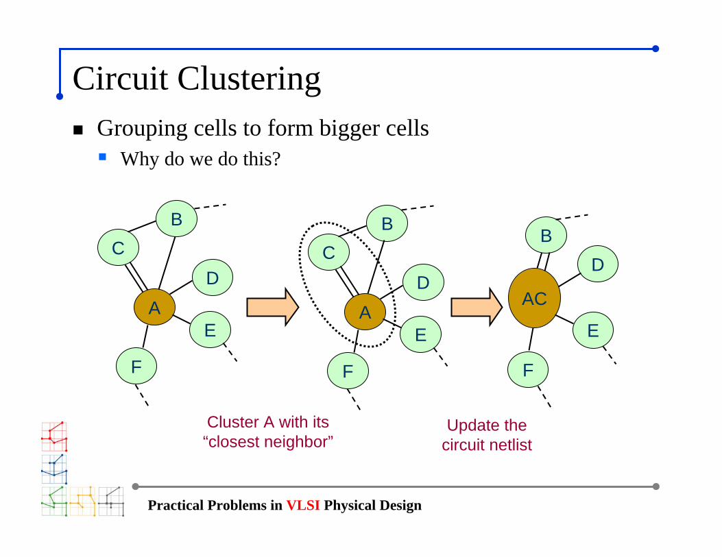
Density MetricDesire high “density” in each cluster
Applied to a single cluster
C1
e6
e3 e5
e4e1 v1
v2
v3
e2
)()()()()()()(/)()(
321
5431
1 1vsvsvsewewewvsewCDEN
Ce Cv ++++
== ∑ ∑∈ ∈

Practical Problems in VLSI Physical Design
Previous WorksCutsize-oriented
(K, I)-connectivity algorithms [Garber-Promel-Steger 1990]Random-walk based algorithm [Cong et al 1991; Hagen-Kahng 1992]Multicommodity-Flow based algorithm [Yeh-Cheng-Lin 1992]Clique based algorithm [Bui 1989; Cong-Smith 1993] Multi-level clustering [Karypis-Kumar, DAC97; Cong-Lim, ASPDAC’00]
Delay-orientedFor combinational circuits: [Lawler-Levitt-Turner 1969; Murgai-Brayton-Sanjiovanni 1991; Rajaraman-Wong 1995; Cong-Ding 1992]For sequential circuits: [Pan et al, TCAD’99; Cong et al, DAC’99]Signal flow based clustering [Cong-Ding, DAC’93; Cong et al ICCAD’97]
Practical Problems in VLSI Physical Design
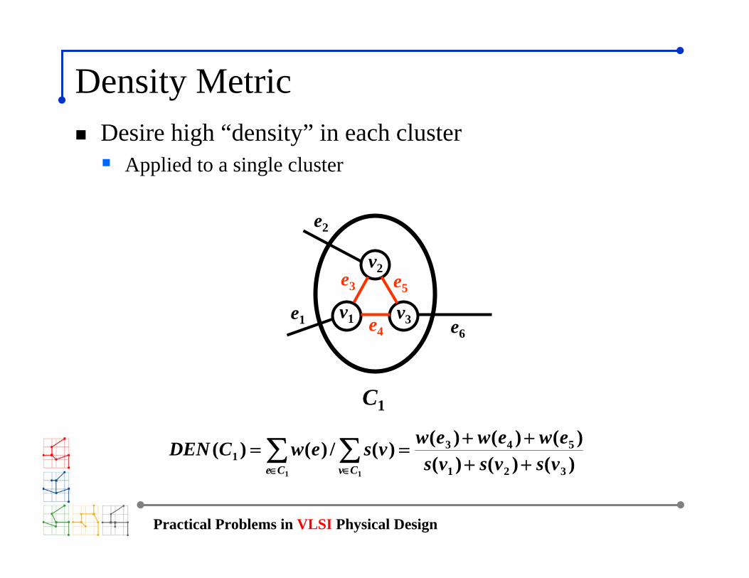
Lawler’s Labeling AlgorithmAssumption:
Cluster size ≤ K; intra-cluster delay = 0; inter-cluster delay = 1
Objective: Find a clustering of minimum delayPhase 1: Label all nodes in topological order
For each PI node v, L(v)= 0;For each non-PI node v
p = maximum label of predecessors of vXp = set of predecessors of v with label pif |Xp| < K then L(v) = p; else L(v) = p+1
Phase 2: Form clustersStart from PO to generate necessary clustersNodes with the same label form a cluster
p-1
Xpp-1
v
p-1
p
p

Practical Problems in VLSI Physical Design
Rajaraman-Wong AlgorithmFirst optimal algorithm that solves delay-oriented clustering problem under general delay modelGiven
DAG, cluster size limit
FindOptimal clustering that minimizes maximum PI-PO path delay
Delay modelNode delay = d, intra-cluster delay = 0; inter-cluster delay = DBetter than “unit delay model” used in Lawler
Node duplication is allowed

Practical Problems in VLSI Physical Design
Rajaraman-Wong AlgorithmInitialization phase
Compute n × n matrix Δ(x,v): all-pair max-delay value from output of x to output of v, using node delay onlySet label(PI) = delay(PI), label(non-PI) = 0
Labeling PhaseCompute label based on topological order of the nodesLabel denotes max delay from any PI to the nodeClustering info is also computed during labeling
Clustering PhaseActual grouping and duplication occurDone based on reserve topological order

Practical Problems in VLSI Physical Design
Labeling for Node v

Practical Problems in VLSI Physical Design
What is going on?

Practical Problems in VLSI Physical Design
Clustering Phase
Practical Problems in VLSI Physical Design Rajaraman-Wong Algorithm (1/8)
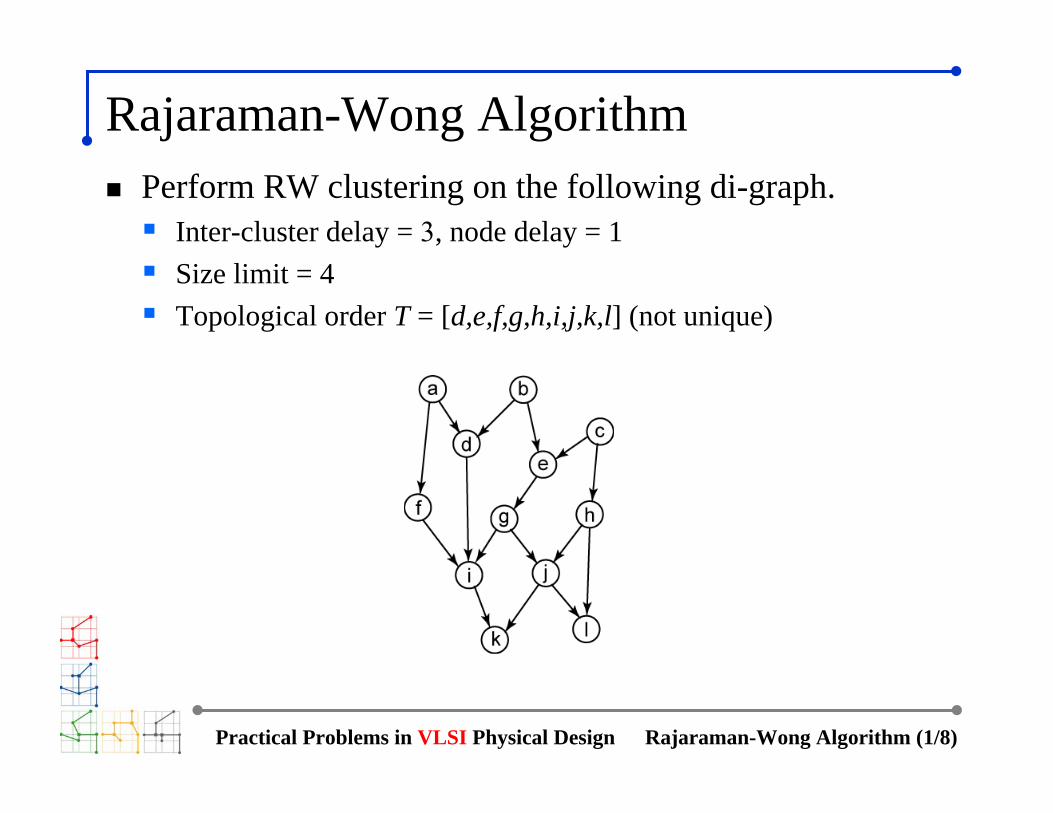
Perform RW clustering on the following di-graph.Inter-cluster delay = 3, node delay = 1Size limit = 4Topological order T = [d,e,f,g,h,i,j,k,l] (not unique)
Rajaraman-Wong Algorithm
Practical Problems in VLSI Physical Design Rajaraman-Wong Algorithm (2/8)
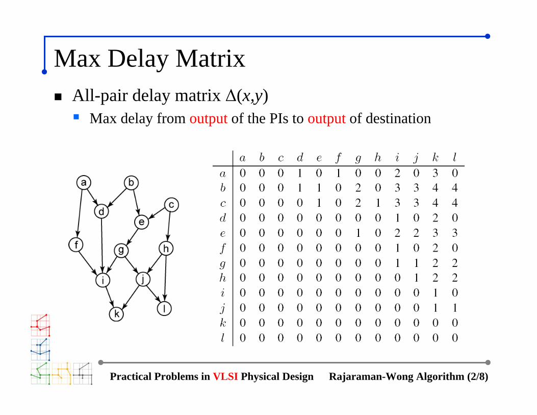
Max Delay MatrixAll-pair delay matrix Δ(x,y)
Max delay from output of the PIs to output of destination

Practical Problems in VLSI Physical Design Rajaraman-Wong Algorithm (3/8)
Label and Clustering ComputationCompute l(d) and cluster(d)

Practical Problems in VLSI Physical Design Rajaraman-Wong Algorithm (4/8)
Label ComputationCompute l(i) and cluster(i)
Practical Problems in VLSI Physical Design Rajaraman-Wong Algorithm (5/8)
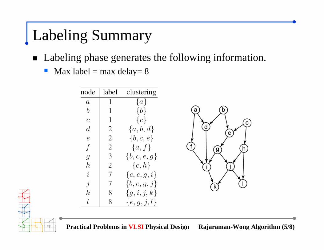
Labeling SummaryLabeling phase generates the following information.
Max label = max delay= 8
Practical Problems in VLSI Physical Design Rajaraman-Wong Algorithm (6/8)
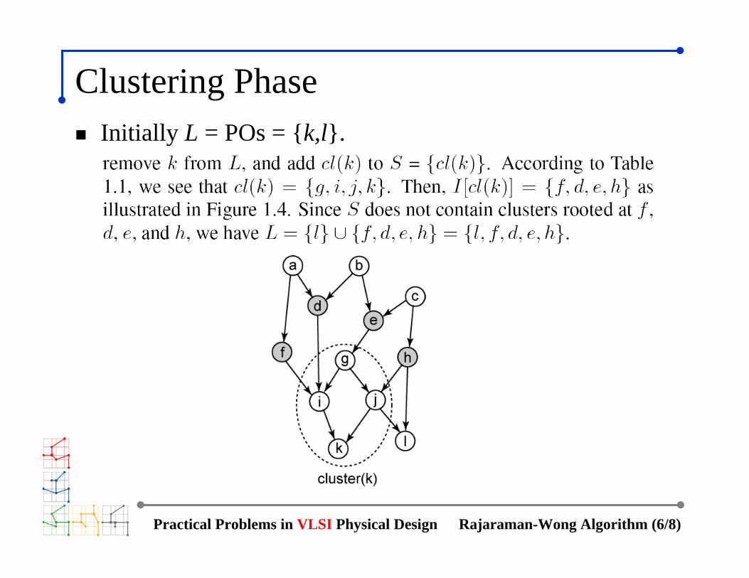
Clustering PhaseInitially L = POs = {k,l}.

Practical Problems in VLSI Physical Design Rajaraman-Wong Algorithm (7/8)
Clustering SummaryClustering phase generates 8 clusters.
8 nodes are duplicated
Practical Problems in VLSI Physical Design Rajaraman-Wong Algorithm (8/8)
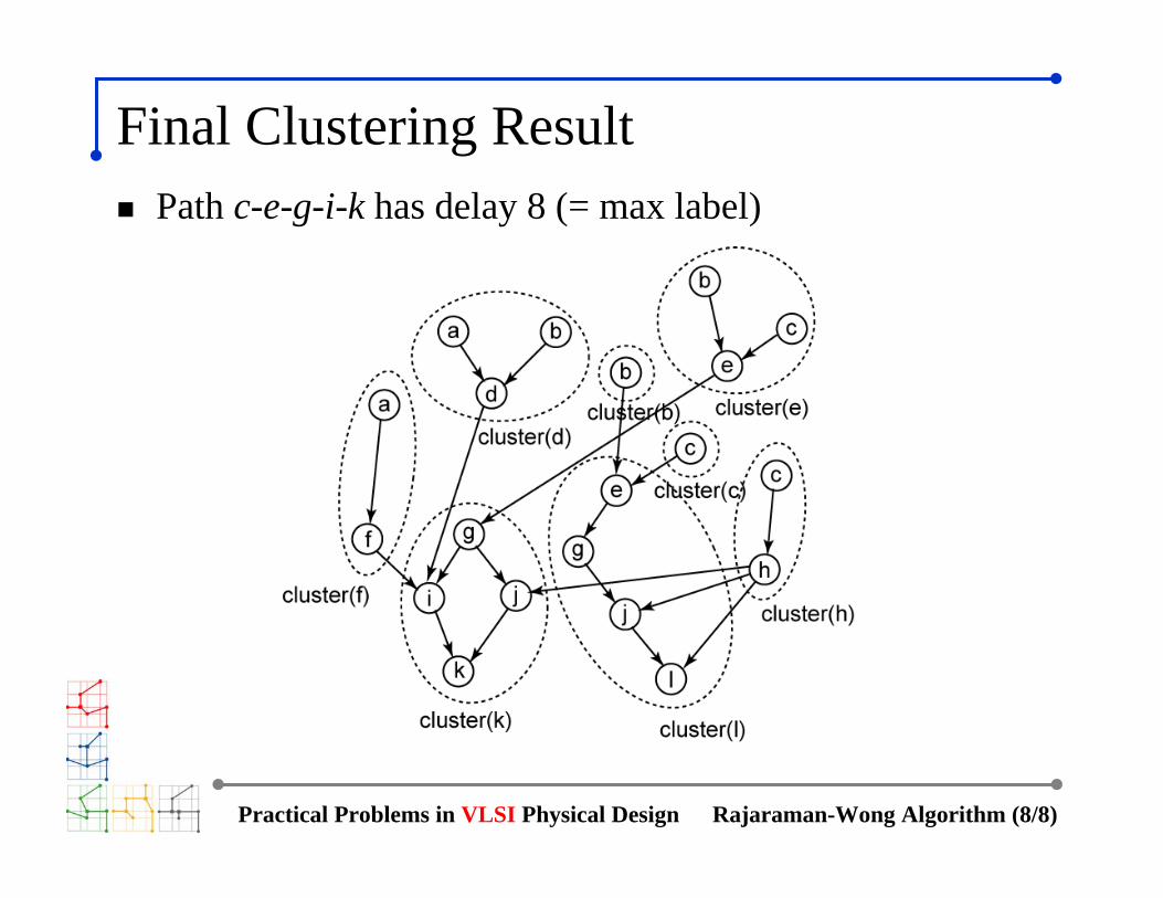
Final Clustering ResultPath c-e-g-i-k has delay 8 (= max label)

Practical Problems in VLSI Physical Design
Probing FurtherRajaraman-Wong Algorithm
[Yang and Wong, 1994]: finds set of nodes to be replicated so that cutsize is minimized[Vaishnav and Pedram, 1995]: minimizes power under delay-optimal clustering properties[Yang and Wong, 1997]: performed delay-optimal clustering under area and/or pin constraint[Pan et at, 1998]: performed delay-optimal clustering with retiming for sequential circuits[Cong and Romesis, 2001]: developed heuristic for two-level delay-oriented clustering problem

Multi-level Paradigm• Combination of Bottom-up and Top-down Methods
– From coarse-grain into finer-grain optimization– Successfully used in partial differential equations, image
processing, combinatorial optimization, etc, and circuit partitioning.
Coarsening Uncoarsening
Initial Partitioning

General Framework• Step 1: Coarsening
– Generate hierarchical representation of the netlist
• Step 2: Initial Solution Generation– Obtain initial solution for the top-level clusters– Reduced problem size: converge fast
• Step 3: Uncoarsening and Refinement– Project solution to the next lower-level (uncoarsening)– Perturb solution to improve quality (refinement)
• Step 4: V-cycle– Additional improvement possible from new clustering– Iterate Step 1 (with variation) + Step 3 until no further gain

V-cycle Refinement• Motivation
– Post-refinement scheme for multi-level methods– Different clustering can give additional improvement
• Restricted Coarsening– Require initial partitioning– Do not merge clusters in different partition– Maintain cutline: cutsize degradation is not possible
• Two Strategies: V-cycle vs. v-cycle– V-cycle: start from the bottom-level– v-cycle: start from some middle-level– Tradeoff between quality vs. runtime

Application in Partitioning• Multi-level Partitioning
– Coarsening engine (bottom-up)• Unrestricted and restricted coarsening• Any bottom-up clustering algorithm can be used• Cutsize oriented (MHEC, ESC) vs. delay oriented (PRIME)
– Initial partitioning engine• Move-based methods are commonly used
– Refinement engine (top-down)• Move-based methods are commonly used• Cutsize oriented (FM, LR) vs. delay oriented (xLR)
• State-of-the-art Algorithms– hMetis [DAC97] and hMetis-Kway [DAC99]

hMetis Algorithm• Best Bipartitioning Algorithm [DAC97]
– Contribution: 3 new coarsening schemes for hypergraphs
Original Graph Edge Coarsening
Edge Coarsening = heavy-edge maximal matching1. Visit vertices randomly2. Compute edge-weights (=1/(|n|-1)) for all unmatched neighbors3. Match with an unmatched neighbor via max edge-weight

hMetis Algorithm (cont)
• Best Bipartitioning Algorithm [DAC97]– Contribution: 3 new coarsening schemes for hypergraphs
Hyperedge Coarsening Modified Hyperedge Coarsening
Hyperedge Coarsening = independent hyperedge merging1. Sort hyperedges in non-decreasing order of their size2. Pick an hyperedge with no merged vertices and merge
Modified Hyperedge Coarsening = Hyeredge Coarsening + post process1. Perform Hyperedge Coarsening2. Pick a non-merged hyperedge and merge its non-merged vertices

hMetis-Kway Algorithm• Multiway Partitioning Algorithm [DAC99]
– New coarsening: First Choice (variant of Edge Coarsening)• Can match with either unmatched or matched neighbors
– Greedy refinement• On-the-fly gain computation• No bucket: not necessarily the max-gain cell moves• Save time and space requirements
Original Graph First Choice

hMetis Results• Bipartitioning on ISPD98 Benchmark Suite
1.61
1.211.03 1
0
0.4
0.8
1.2
1.6
Scal
ed C
utsiz
e
FM LR LR/ESC hMetis
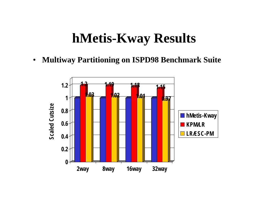
hMetis-Kway Results• Multiway Partitioning on ISPD98 Benchmark Suite
1.21.03
1.191.02
1.181.01
1.15
0.97
0
0.2
0.4
0.6
0.8
1
1.2
Scale
d Cu
tsize
2way 8way 16way 32way
hMetis-KwayKPM/LRLR/ESC-PM

Practical Problems in VLSI Physical Design Multi-level Coarsening (1/11)
Perform Edge Coarsening (EC)Visit nodes and break ties in alphabetical orderExplicit clique-based graph model is not necessary
Multi-level Coarsening Algorithm

Practical Problems in VLSI Physical Design Multi-level Coarsening (2/11)
Edge Coarsening

Practical Problems in VLSI Physical Design Multi-level Coarsening (3/11)
Edge Coarsening (cont)
Practical Problems in VLSI Physical Design Multi-level Coarsening (4/11)
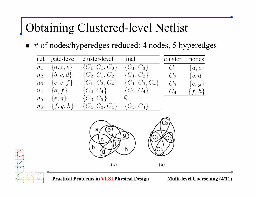
Obtaining Clustered-level Netlist# of nodes/hyperedges reduced: 4 nodes, 5 hyperedges

Practical Problems in VLSI Physical Design Multi-level Coarsening (5/11)
Hyperedge CoarseningInitial setup
Sort hyper-edges in increasing size: n4, n5, n1, n2, n3, n6
Unmark all nodes

Practical Problems in VLSI Physical Design Multi-level Coarsening (6/11)
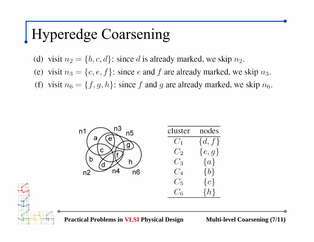
Hyperedge Coarsening
Practical Problems in VLSI Physical Design Multi-level Coarsening (7/11)
Hyperedge Coarsening

Practical Problems in VLSI Physical Design Multi-level Coarsening (8/11)
Obtaining Clustered-level Netlist# of nodes/hyperedges reduced: 6 nodes, 4 hyperedges

Practical Problems in VLSI Physical Design Multi-level Coarsening (9/11)
Modified Hyperedge CoarseningRevisit skipped nets during hyperedge coarsening
We skipped n1, n2, n3, n6
Coarsen un-coarsened nodes in each net

Practical Problems in VLSI Physical Design Multi-level Coarsening (10/11)
Modified Hyperedge Coarsening
Practical Problems in VLSI Physical Design Multi-level Coarsening (11/11)
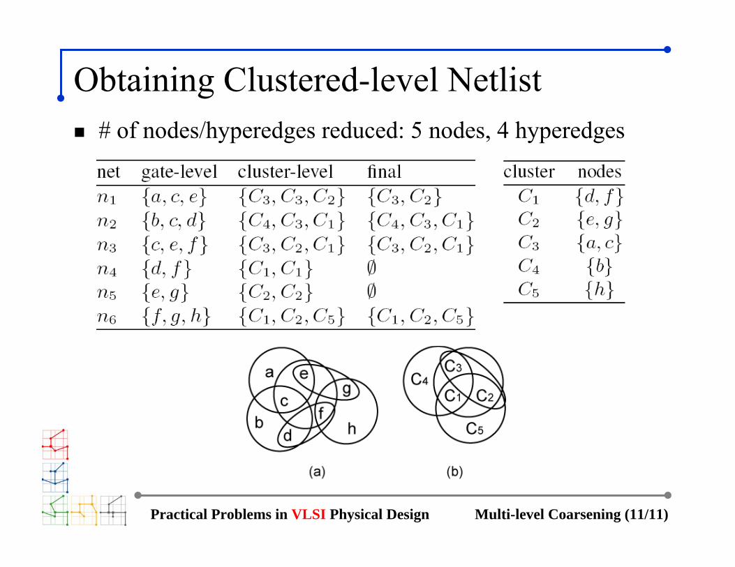
Obtaining Clustered-level Netlist# of nodes/hyperedges reduced: 5 nodes, 4 hyperedges
Top Related