


Languages
Pages
Legal


8.1
Chapter 8
Robust Designs

8.2
Robust Designs
C S
R O
R
Focus: A Few Primary Factors Output: Best/Robust Settings

8.3
Robust Designs
C S
R O
RI/O Arrays
Assembled Designs

8.4
Robust Experimentation
• Try to reduce the variation in the product.process, not just set it on target.
• Try to find conditions of design factors which make the product/process insensitive or robust to its environment.
• The idea was championed by Genichi Taguchi.– Taguchi really opened a whole area that previously had been
talked about only by a few very applied people.– His methodology is heavily dependent on design of experiments,
but he wanted to look at not just the mean but also the variance.

8.5
Classification of Factors
• Control Factors–Design factors that are to be set at optimal levels to improve quality and reduce sensitivity to noise
– Dimensions of parts, type of material, etc
• Noise Factors–Factors that represent the noise that is expected in production or in use
– Dimensional variation– Operating Temperature
• Adjustment Factor – Affects the mean but not the variance of a response
– Deposition time in silicon wafer fabrication
• Signal Factors – Set by the user to communicate desires of the user
– Position of the gas pedal

8.6
Example: Ignition Coil
Most automotive sub-assemblies like the alternator, the ignition coil, and the electronic control module must undergo testing to determine if they are resistant to salt water
that may be splashed on them from the read. An automotive supplier is testing an ignition coil to determine if it will withstand salt water. The
following factors are tested:

8.7
Control or Noise Factor?
NChicago PinkDetroit BlueType of Salt
N5 hrs.1 hr.Exposure Time
C0.03”0.02”Seal Thickness
CVinylSiliconeSeal Material
N20 PSI10 PSIWater Pressure
N15ºC5ºCWater Temperature
N20%10%Concentration
Of Salt
CPolypropylen ($20/lb)
Polyethylene ($9/lb)
Housing Material
Factor TypeHigh LevelLow LevelFactor

8.8
Taguchi’s Design of Experiments Ideas
• Use Orthogonal Arrays (e.g., Resolution III Fractional Factorials) that only estimate main effects and specified interactions.
• Intentionally vary the noise factors so that you choose a set of conditions that will work well in the face of the noise expected in the actual application.
• Inner/Outer Arrays– Two statistical designs per experiment:
» A design in the control factors called an inner array» A design in the noise factors called an outer array
– Good for estimating CxN Factor Interactions.

8.9
Taguchi’s Analysis IdeasSignal to Noise Ratio
• A single response which makes a tradeoff between setting the mean to a desirable level while keeping the variance low.
• Always try to MAXIMIZE a SN Ratio• There are three types:
– Smaller is Better– Target is Best
– Larger is Better

8.10
Smaller is Better
• Maximize the signal to noise ratio• Run a confirmatory experiment
SNy
ny
n
nsS
j
j
= −
= − + −
∑10 10
122 2log log
The signal to noise ratio confounds the mean and the variance together and assumes that the variance is proportional to the mean.

8.11
Examples with the same SNS Ratio
0
5
10
15
20
0 1 2 3 4 5
Y-V
alue
s
0
5
10
15
20
0 1 2 3 4 5
Y-V
alue
s
0
5
10
15
20
0 1 2 3 4 5
Y-V
alue
s
0
5
10
15
20
0 1 2 3 4 5
Y-V
alue
s
1 10 12 3 12 10 6 7 13 10 14.6 11 14 10 3 15 20
SNS -20 -20.0234 -20.0432 -20.0325
8.12
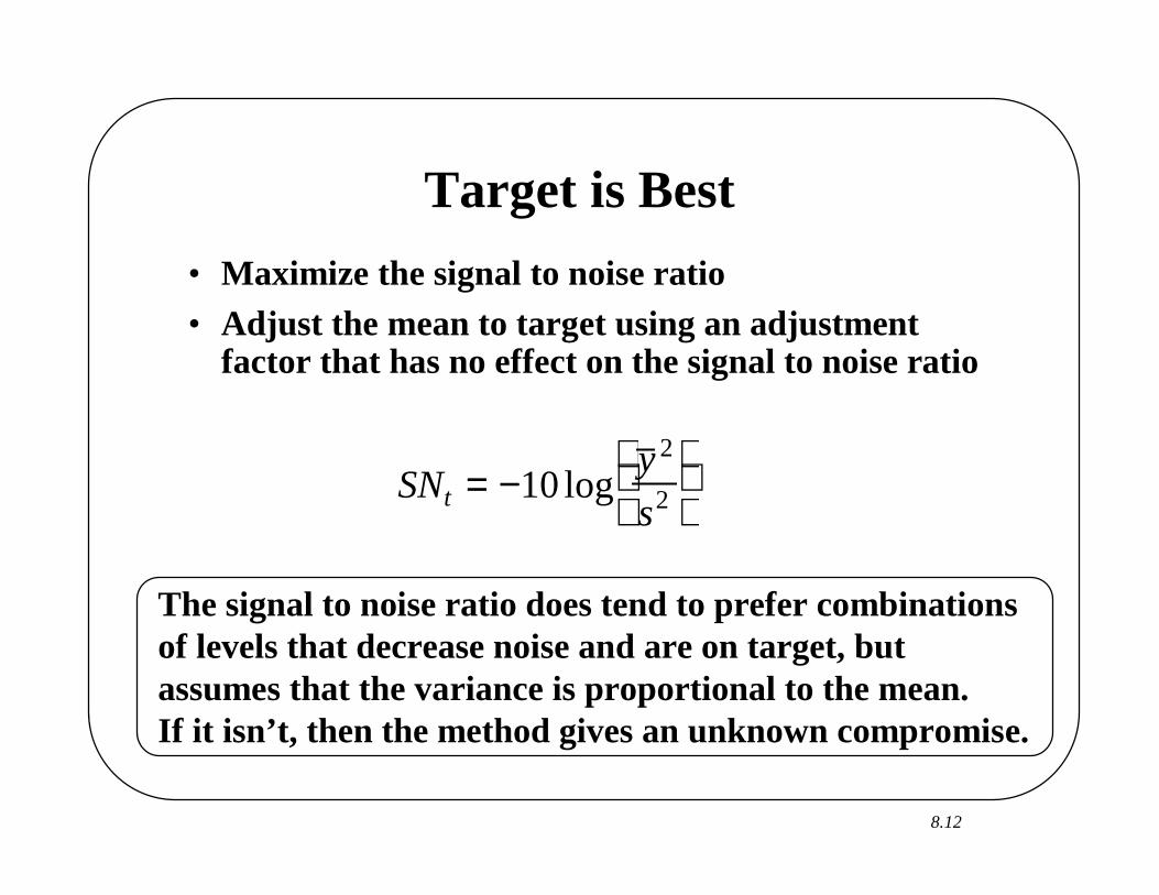
Target is Best
SNt = −10 logy 2
s2
• Maximize the signal to noise ratio• Adjust the mean to target using an adjustment
factor that has no effect on the signal to noise ratio
The signal to noise ratio does tend to prefer combinations of levels that decrease noise and are on target, but assumes that the variance is proportional to the mean. If it isn’t, then the method gives an unknown compromise.

8.13
Larger is Better
SNy
nLjj
= −
∑10
12log
• Maximize the signal to noise ratio• Run a confirmation
The signal to noise ratio again confounds the mean and the variance together and assumes that the variance is proportional to the mean.

8.14
Sources of Variance
• Measurement• Setup• Blocks• Noise Factors
– Manufacturing Variation– Field Conditions

8.15
Repeats
x1 x2 x3 y1 y2 y3
– – – y 11 y 21 y 31
+ – – y 12 y 22 y 32
– + – y 13 y 23 y 33
+ + – y 14 y 24 y 34
– – + y 15 y 25 y 35
+ – + y 16 y 26 y 36
– + + y 17 y 27 y 37
+ + + y 18 y 28 y 38
σ2 represents measurement error
8.16
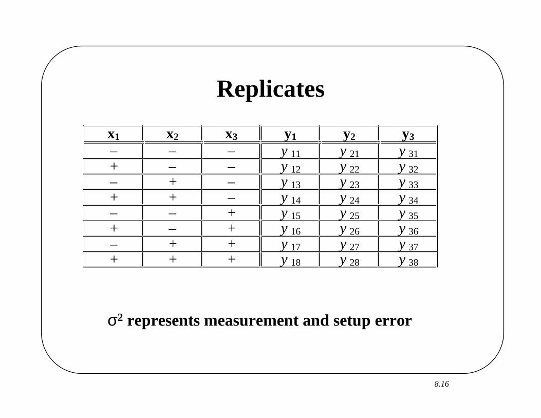
Replicates
x1 x2 x3 y1 y2 y3
– – – y 11 y 21 y 31
+ – – y 12 y 22 y 32
– + – y 13 y 23 y 33
+ + – y 14 y 24 y 34
– – + y 15 y 25 y 35
+ – + y 16 y 26 y 36
– + + y 17 y 27 y 37
+ + + y 18 y 28 y 38
σ2 represents measurement and setup error

8.17
Blocks
x1 x2 x3 Machine 1 Machine 2 Machine 3– – – y 11 y 21 y 31
+ – – y 12 y 22 y 32
– + – y 13 y 23 y 33
+ + – y 14 y 24 y 34
– – + y 15 y 25 y 35
+ – + y 16 y 26 y 36
– + + y 17 y 27 y 37
+ + + y 18 y 28 y 38
σ2 represents variance between blocks and measurement and setup error.

8.18
Noise Factors
x1 x2 x3 Temp1 Temp2 Temp3– – – y 11 y 21 y 31
+ – – y 12 y 22 y 32
– + – y 13 y 23 y 33
+ + – y 14 y 24 y 34
– – + y 15 y 25 y 35
+ – + y 16 y 26 y 36
– + + y 17 y 27 y 37
+ + + y 18 y 28 y 38
σ2 represents variance expected in the field due to field conditions and measurement and setup error. The idea of robustness is to set the x’s to minimize the variance, while keeping the average response at a desired level.

8.19
I/O (crossed) ArrayAn Inner Array of Control Factors and
an Outer Array of Noise FactorsLength – + – +Temp – – + +
Gage Wraps Geom. y1 y2 y3 y4
– – – y 11 y 21 y 31 y 41
+ – – y 12 y 22 y 32 y 42
– + – y 13 y 23 y 33 y 43
+ + – y 14 y 24 y 34 y 44
– – + y 15 y 25 y 35 y 45
+ – + y 16 y 26 y 36 y 46
– + + y 17 y 27 y 37 y 47
+ + + y 18 y 28 y 38 y 48
σ2 represents variance expected in the field and measurement and setup error.

8.20
Analysis
• Taguchi suggests SN Ratios.
• We could analyze the average and the standard deviation separately.
• We could define some other summary response– Minimize the range or the curvature
• We could include effects for each y and explain each one individually like we do with blocks.

8.21
Analyzing the Mean and Standard Deviation Separately
• For each row of y’s, we can take the mean of the row as one response and the log of the standard deviation as another response.
• The log is used because the variance of the standard deviation is not constant as the standard deviation increases.
• We then try to compromise between setting the mean to a desirable level and reducing the standard deviation.
• Effects on the mean are called Location Effects. • Effects on the standard deviation are called
Dispersion Effects

8.22
Analysis of I/O (Crossed) Arrays
• When we have I/O array there will be three types of effects
– Control Main Effects and Interactions– Noise Main Effects and Interactions
– Control by Noise Interactions
• Depending on HOW WE RUN THE EXPERIMENT, the different effects may have different variances.
• Suppose that there are n runs in the control array and m runs in the noise array. There will be a total of nm data points.

8.23
Example: Cake Mix Example
• Amounts of ingredients like egg, shortening and flour are the control factors (n levels in the control array)
• Time and Temperature in baking are the noise factors (m levels in the noise array)
Temp – + – +time – – + +
Flour Shrtg Egg– – – 1.3 1.6 1.2 3.1+ – – 2.2 5.5 3.2 6.5– + – 1.3 1.2 1.5 1.7+ + – 3.7 3.5 3.8 4.2– – + 1.6 3.5 2.3 4.4+ – + 4.1 6.1 4.9 6.3– + + 1.9 2.4 2.6 2.2+ + + 5.2 5.8 5.5 6.0
8.24
How do we run the experiment?
1. Fully Randomized
2. Split Plot
3. Strip Block

8.25
1. Fully Randomized
• Make nm products and test them each separately.

8.26
2. Split Plot
• Experiments where you can’t or don’t think it is worth it to fully randomize the experiment
• Used when there are certain effects that you want to estimate with high precision. (like blocking)
• Often needed when some factors are “hard to change” and others are “easy to change”
• I/O arrays are often but not always run as split plot experiments

8.27
Split Plot Variance
• Whole-plot effects have high variance. • Sub-plot effects have lower variance.• Only effects that have the same variance should be
put on the same normal plot.

8.28
2a. Split Plot ArrangementControl Factors as Whole-Plot Effects
• Mix up n big batches of batter• Split each batch into m parts• Bake m x n cakes in m x n oven runs• All Control Effects have error due to batch error
and due to random error • All Noise Effects and CxN interactions have only
random error • 2 Normal Plots

8.29
2b. Split Plot ArrangementControl Factors as Sub-Plot Effects
• Mix up m x n batches of batter• Bake all n batter types together under each set of
noise conditions• Bake m x n cakes in m oven runs• All Noise Effects have error due to oven error and
due to random error • All Control Effects and CxN interactions have only
random error • 2 Normal Plots

8.30
3. Strip Block Arrangement• Mix up n batches of batter• Split each batch into m parts• Bake all n batter types together under each set of
noise conditions• Bake m x n cakes in m oven runs• All Noise Effects have error due to oven error and
due to random error • All Control Effects have error due to batch error
and due to random error • CxN interactions have only random error • 3 Normal Plots

8.31
The purpose of each of these configurations is to reduce the experimental cost and target certain effects to have higher
precision of measurement.

8.32
HOW WE RUN THE EXPERIMENT
• Fully Randomize – Make nm different products and test them each separately– One normal plot with all effects
• Split Plot– Make n different products and test each product in nm separate
tests.» Two normal plots (1) Control (2) Noise and CxN
– Make nm different products and test them in groups of n in m tests.
» Two normal plots (1) Control and CxN (2) Noise
• Strip Block– Make n different products and test them each in m tests.
» Three normal plots (1) Control (2) CxN (3) Noise

8.33
-11
11-1-1
60
50
40
30
20
Temp
Control by Noise Factor InteractionsM
oist
ness
Set Control Factor(e.g. Shortening) to Low Level
Noise Factor (e.g. Temp.)
Shortening
Interaction between Shortening and Temperature

8.34
Control by Noise Factor InteractionsM
oist
ness
Set Control Factor(e.g. Flour) to Middle Level
Noise Factor (e.g. Temp.)
Flour
Interaction between Flour and Temperature
-11
11-1-1
60
50
40
30
20
Temp
Mea
n

8.35
Control by Noise Factor InteractionsM
oist
ness
Set the AdjustmentFactor (e.g. Egg) to Set Mean on Target
Noise Factor (e.g. Temp.)
Egg
Interaction between Egg and Temperature
-11
11-1-1
60
50
40
30
20
Temp
Mea
n

8.36
I/O Arrays and Control by Noise Interactions
• I/O arrays always estimate the CxN Interactions with the highest precision (lowest variance).
• Sometimes the I/O array design is larger than it needs to be to get the same resolution
• However, if we are interested in estimating CxNinteractions, then an I/O array design can be a very good design.

8.37
Confounding in I/O Arrays
• Same as in standard arrays– Write down identity relationships from generators– Multiply out all possible combinations to get defining
relation– Multiply defining relation by any effect to get alias structure– Equivalently we could get the individual defining relations
and multiply every possible pair of terms
• Resolution of a crossed array experiment is the minimum of the resolutions of the individual arrays
– RC = Resolution of Control Array– RN = Resolution of Noise Array

8.38
Defining Relation I=ABC=PQR=ABCPQR
P – + – +Q – – + +
R=PQ + – – +A B C=AB y1 y2 y3 y4
– – + y 11 y 21 y 31 y 41
+ – – y 12 y 22 y 32 y 42
– + – y 13 y 23 y 33 y 43
+ + + y 14 y 24 y 34 y 44
Notice that as long as each individual array is Resolution III the shortest word containing both control and noise factors will have length 6.

8.39
Confounding Pattern
• A=BC=APQR=BCPQR• B=AC=BPQR=ACPQR• C=AB=CPQR=ABPQR• P=ABCP=QR=ABCQR• Q=ABCQ=PR=ABCPR• R=ABCR=PQ=ABCPQ• AP=BCP=AQR=BCQR• AQ=BCQ=APR=BCPR• AR=BCR=APQ=BCPQ
• BP=ACP=BQR=ACQR• BQ=ACQ=BPR=ACPR• BR=ACR=BPQ=ACPQ• CP=ABP=CQR=BCQR• CQ=ABQ=CPR=ABPR• CR=ABR=CPQ=ABPQ

8.40
Control by Noise Factor Interactions will be confounded with interactions of
order Min(RC, RN).
So, if both arrays have Resolution III then CxN interactions will be confounded with three factor
interactions.
8.41
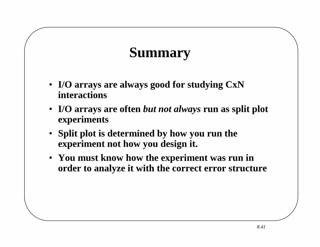
Summary
• I/O arrays are always good for studying CxNinteractions
• I/O arrays are often but not always run as split plot experiments
• Split plot is determined by how you run the experiment not how you design it.
• You must know how the experiment was run in order to analyze it with the correct error structure

8.42
My Recommendations
• Think about the idea of robustness in the planning stage of your experiment and choose the response accordingly.
• If you choose to reduce variance, then make sure that the variance that you are reducing is the variance that you want to reduce and that it is worth the experimental effort.
• Analyze the mean and variance separately and make decisions concerning the tradeoffs between reducing variance and achieving the desired mean value.
• Use Inner and Outer Arrays to estimate Control by Noise Interactions for designing Robust Products and Processes.

8.43
Assembled Designs
Parameters:r = # of Design Pointsn = # of observations per Treatment Combination (assume constant)s = # of different structures used in the designBT = total number of Batches
x1
x3
x2
1 2
3 4
5 6
7 8
A class of experimental design for estimating location effects, dispersion effects, and variance components.
“Works for anything that involves making batches and taking observations ”
r = 8n = 4s = 2
BT = 20

8.44
Notation for Assembled Designs
Example: 23 design, Splitting Generator = ABC, r=8, s=2, B1=4, B2=3, n=6
Must have design points ordered in some way.∑
=
s
j
jj1
} structure with points@{design structure
D e s ig n P o in t A B C A B C S tr u c tu r e 1 - - - - (2 ,1 ,1 ) 2 + - - + (2 ,2 ) 3 - + - + (2 ,2 ) 4 + + - - (2 ,1 ,1 ) 5 - - + + (2 ,2 ) 6 + - + - (2 ,1 ,1 ) 7 - + + - (2 ,1 ,1 ) 8 + + + + (2 ,2 )
,5,8}(2,2)@{2,3 ,4,6,7}(2,1,1)@{1 +
Top Related