


Languages
Pages
Legal

Casual 3D Photography
PETER HEDMAN, University College London*SUHIB ALSISAN, FacebookRICHARD SZELISKI, FacebookJOHANNES KOPF, Facebook
Casual 3D photo capture Color Depth Normal map
Reconstruction
Geometry-aware Lighting
Example Effects
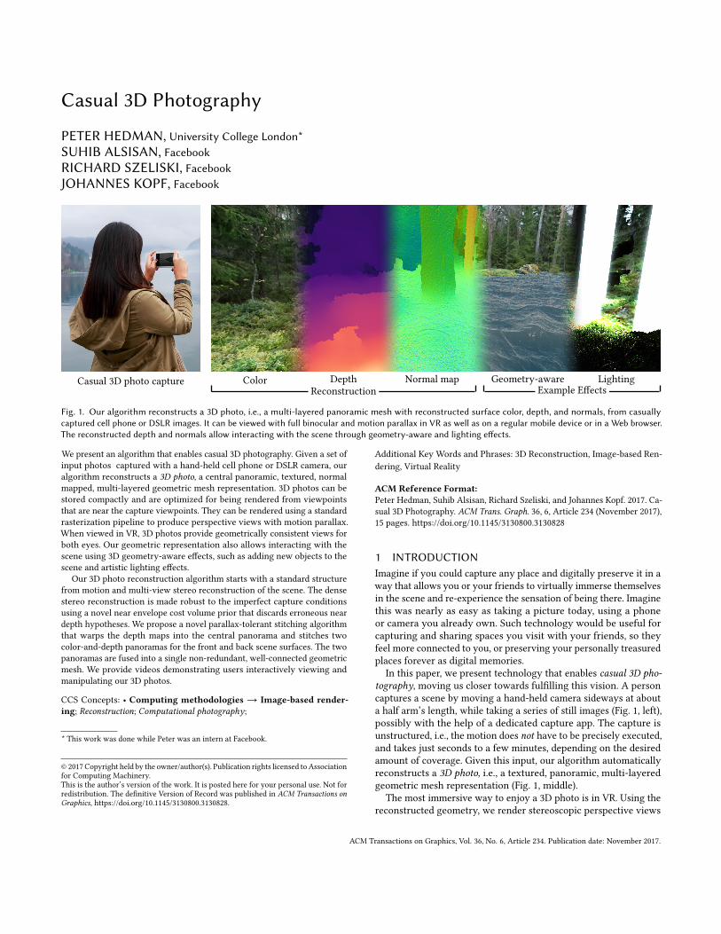
Fig. 1. Our algorithm reconstructs a 3D photo, i.e., a multi-layered panoramic mesh with reconstructed surface color, depth, and normals, from casuallycaptured cell phone or DSLR images. It can be viewed with full binocular and motion parallax in VR as well as on a regular mobile device or in a Web browser.The reconstructed depth and normals allow interacting with the scene through geometry-aware and lighting effects.
We present an algorithm that enables casual 3D photography. Given a set of
input photos captured with a hand-held cell phone or DSLR camera, our
algorithm reconstructs a 3D photo, a central panoramic, textured, normal
mapped, multi-layered geometric mesh representation. 3D photos can be
stored compactly and are optimized for being rendered from viewpoints
that are near the capture viewpoints. They can be rendered using a standard
rasterization pipeline to produce perspective views with motion parallax.
When viewed in VR, 3D photos provide geometrically consistent views for
both eyes. Our geometric representation also allows interacting with the
scene using 3D geometry-aware effects, such as adding new objects to the
scene and artistic lighting effects.
Our 3D photo reconstruction algorithm starts with a standard structure
from motion and multi-view stereo reconstruction of the scene. The dense
stereo reconstruction is made robust to the imperfect capture conditions
using a novel near envelope cost volume prior that discards erroneous near
depth hypotheses. We propose a novel parallax-tolerant stitching algorithm
that warps the depth maps into the central panorama and stitches two
color-and-depth panoramas for the front and back scene surfaces. The two
panoramas are fused into a single non-redundant, well-connected geometric
mesh. We provide videos demonstrating users interactively viewing and
manipulating our 3D photos.
CCS Concepts: • Computing methodologies → Image-based render-ing; Reconstruction; Computational photography;
* This work was done while Peter was an intern at Facebook.
© 2017 Copyright held by the owner/author(s). Publication rights licensed to Association
for Computing Machinery.
This is the author’s version of the work. It is posted here for your personal use. Not for
redistribution. The definitive Version of Record was published in ACM Transactions onGraphics, https://doi.org/10.1145/3130800.3130828.
Additional Key Words and Phrases: 3D Reconstruction, Image-based Ren-
dering, Virtual Reality
ACM Reference Format:Peter Hedman, Suhib Alsisan, Richard Szeliski, and Johannes Kopf. 2017. Ca-
sual 3D Photography. ACM Trans. Graph. 36, 6, Article 234 (November 2017),
15 pages. https://doi.org/10.1145/3130800.3130828
1 INTRODUCTIONImagine if you could capture any place and digitally preserve it in a
way that allows you or your friends to virtually immerse themselves
in the scene and re-experience the sensation of being there. Imagine
this was nearly as easy as taking a picture today, using a phone
or camera you already own. Such technology would be useful for
capturing and sharing spaces you visit with your friends, so they
feel more connected to you, or preserving your personally treasured
places forever as digital memories.
In this paper, we present technology that enables casual 3D pho-tography, moving us closer towards fulfilling this vision. A person
captures a scene by moving a hand-held camera sideways at about
a half arm’s length, while taking a series of still images (Fig. 1, left),
possibly with the help of a dedicated capture app. The capture is
unstructured, i.e., the motion does not have to be precisely executed,and takes just seconds to a few minutes, depending on the desired
amount of coverage. Given this input, our algorithm automatically
reconstructs a 3D photo, i.e., a textured, panoramic, multi-layered
geometric mesh representation (Fig. 1, middle).
The most immersive way to enjoy a 3D photo is in VR. Using the
reconstructed geometry, we render stereoscopic perspective views
ACM Transactions on Graphics, Vol. 36, No. 6, Article 234. Publication date: November 2017.
234:2 • Hedman et. al.
that correctly react to tracked user head motion, i.e., provide binoc-
ular and motion-parallax depth cues. On non-VR displays such as
smart phones, we can still show motion parallax by rendering from
viewpoints on a sphere fitted to the estimated input camera loca-
tions. Our geometric representation enables interacting with the 3D
photo through geometry-aware and artistic lighting effects (Fig. 1,
right).
We specifically designed our representation and reconstruction
algorithms for as “casual” as possible capture. We do not require
the user to capture a scene from all angles, but just an arc around a
single viewpoint. As a result, our 3D photos are most suited for an
“armchair exploration” scenario. They look best when viewed from
within a volume around the viewpoints that were spanned during
capture.
An alternative representation often used for VR capture is the
omnidirectional stereo representation (ODS) for capturing and ren-
dering stereoscopic panoramic images and videos, which uses sep-
arate 360◦panoramas for the left and right eye [Peleg et al. 2001].
These panoramas are captured either by sweeping a regular camera
around a ring [Peleg et al. 2001; Richardt et al. 2013] or from a ring
of overlapping video cameras [Anderson et al. 2016; Facebook 2016].
ODS provides a binocular depth cue by delivering different images
to the eyes, but does not provide motion parallax when the user
turns or moves their head. The rendered views are not in a linear
perspective projection and exhibit distortions such as bent scene
lines and incorrect stereo parallax away from the equator. These
artifacts are described in more detail in Section 2. Our system pro-
vides binocular and motion parallax depth cues, and therefore a
better sense of immersion. Another important difference is that any
incorrectly reconstructed geometry in a 3D photo will still be ren-
dered consistently for both eyes, while artifacts in an ODS produce
inconsistent views that can cause motion sickness.
Multi-view stereo (MVS) [Furukawa and Hernández 2015] algo-
rithms reconstruct a dense and detailed 3D geometric model from a
set of images. This mature field in computer vision has seen over
30 years of research, and several high quality and actively main-
tained software packages implementing state-of-the-art algorithms
are available (see Section 6.2). However, applying these algorithms
directly in our scenario produces unsatisfactory results, for the fol-
lowing reasons: (1) our casually captured images violate many com-
mon assumptions in MVS algorithms leading to geometric artifacts:
they are captured with a narrow baseline, and our scenes are often
not fully static and contain large textureless areas; (2) the geometry
produced by MVS algorithms is not optimized for a specific view-
point and often lacks completeness and detail. Our approach uses
state-of-the-art reconstruction algorithms as core components, but
through several technical innovations, we make them work robustly
in our scenario. We provide extensive comparisons against several
MVS packages in Section 6.2 and the supplementary material.
The reconstruction of a 3D photo starts with estimating input cam-
era poses and a sparse scene model using an off-the-shelf structure-
from-motion algorithm. This is followed by our three major techni-
cal innovations.
(1) A novel near-envelope cost volume prior is used to improve the
robustness of MVS depth map reconstruction by discarding
erroneous nearby depth hypotheses.
(2) A novel parallax-tolerant stitching algorithm warps the depth
maps into a central panoramic domain and stitches two panora-
mas: one for the front and one for the back (occluded) surface
in the scene. Each map is reconstructed in the original image
domain to achieve good alignment of image and depth edges.
These are then rendered with a regular and an inverted z-test
to produce front and back surface warps, which are subse-
quently stitched into corresponding front and back surface
panoramas.
(3) A novel two-layer fusion algorithm that merges the front
and back surface panoramas into a consistent, two-layered,
textured geometric mesh: the 3D photo.
Our 3D photo representation can be rendered on any modern
platform using standard graphics engines. The reconstruction qual-
ity is sufficient for moderate viewpoint changes, roughly within the
volume spanned by the captured images. We have experimented
with a variety of playful geometry-aware and lighting effects that
make use of the reconstructed scene geometry.
We have applied our algorithm to numerous 3D photos captured
with DSLRs and cell phone cameras. Among these are indoor and
outdoor as well as man-made and natural scenes. We compare our
3D photos extensively with results obtained with existing state-of-
the-art reconstruction algorithms, and provide quantitative analysis
using the Virtual Rephotography evaluation method [Waechter et al.
2017]. In the supplementary material, we provide datasets consisting
of input images, results, and intermediate algorithm stage outputs
for all of our scenes, as well as the results and rephotography error
maps for 16 variants of competing methods.
2 PREVIOUS WORKOur work builds on a long tradition of image-based modeling and
rendering, omnidirectional stereo, panoramic image stitching, multi-
view stereo and free-viewpoint video, photogrammetry, surface
normal estimation, and relighting. In this section, we highlight
some of the related work in these areas.
Omnidirectional Stereo: Omnidirectional stereo encompasses a
class of techniques for stitching together a pair of left-eye and right-
eye panoramic images [Anderson et al. 2016; Ishiguro et al. 1990;
Peleg et al. 2001; Richardt et al. 2013]. The original techniques for
generating such images used strips from moving camera images
to create the panoramic images, using either mechanical rotation
[Ishiguro et al. 1990; Peleg and Ben-Ezra 1999] or hand-held images
[Google 2015; Richardt et al. 2013; Zhang and Liu 2015]. More re-
cent systems enable the capture of stereo panoramic videos using
multiple cameras arranged in a ring [Anderson et al. 2016; Facebook
2016].
Unfortunately, omnidirectional stereo images have a number of
drawbacks [Anderson et al. 2016], particularly when applied to full
spherical images. These include:
(1) non-linear perspective: straight lines in the scene are rendered
as bent;
(2) unnatural non-rigid motion: the scene appears to swim or
bend above and below the equator as the viewer turns their
head;
(3) the lack of realistic motion parallax as the head is turned;
ACM Transactions on Graphics, Vol. 36, No. 6, Article 234. Publication date: November 2017.
Casual 3D Photography • 234:3
(4) incorrect stereo parallax away from the equator, most no-
ticeable as the distance to the floor appearing “at infinity”,
resulting in unpleasant vertigo;
(5) the inability to tilt the head sideways and obtain correct binoc-
ular parallax;
(6) un-specified behavior at the poles: a simple 180 vertical sweep
leaves gaps.
There are some other stitching methods that are not specifically
designed for omnistereo but general stereoscopic image pairs. Luo
et al. [2012] describe a method for cloning a manually specified
selection from one stereoscopic image to another, and adjusting the
colors and disparities through iterative gradient-domain blending.
Parallax-tolerant panorama stitching: Some methods warp input
images to stitch artifact-free monocular panoramas [Lin et al. 2016;
Shum and Szeliski 1998; Zaragoza et al. 2013; Zhang and Liu 2014].
Recent work[Zhang and Liu 2015] demonstrates that this approach
also extends to omni-directional stereo. However, this line of work
has not yet produced explicit 3D geometry, making them unable to
produce head-motion parallax in VR.
Panoramas with Depth: An alternative to generating a left-right
pair of panoramic images is to augment a traditional stitched panora-
mic image with depth information [Im et al. 2016]. However, simply
adding a single depth channel to a panorama is not sufficient, be-
cause viewpoint changes can lead to issues at depth discontinuities,
i.e., reveal long stretched triangles or holes.
Zheng et al. [2007] create a layered depth panorama from multi-
ple overlapping images using a cylinder-sweep multi-view stereo
(MVS) algorithm. One problem with Zheng et al’s approach is that
their layers are not connected, which prevents their algorithm from
reproducing sloped surfaces. In addition, our approach of first com-
puting per-image depth maps allows us to use the original images
as references to achieve better edge alignment, and our stitching
step can hide MVS artifacts.
Thatte et al. [2016] describe a representation rendering for ODS
with depth and sketch out capturing and rendering algorithms, but
mostly demonstrate their system with synthetic data and a simple
“proof-of-concept” captured scene, and leave the question of reliable
depth estimation open.
SLAM and depth sensors: Simultaneous Localization and Mapping
(SLAM) methods are able to reconstruct hand-held video [Engel
et al. 2016; Mur-Artal and Tardós 2016]. The sparse or semi-dense
reconstructions created by these methods are useful for render-
ing augmented reality overlays onto video, but more geometry- or
occlusion-aware effects such as the virtual water surface (Figure 1)
or virtual viewpoint changes require dense reconstructions. Dense
SLAM methods [Izadi et al. 2011] usually rely on depth sensor in-
put. [Hedman et al. 2016] use a combination of depth sensors and
multi-view stereo in an image-based rendering system that repro-
duces view-dependent effects and allows for a freely moving camera.
However, their scene representation is expensive to render and this
system requires elaborate, indoor-only capture.
Multi-view Stereo and Free-viewpoint Video: Multi-view stereo
algorithms produce depth maps or surface meshes by matching mul-
tiple overlapping images [Seitz et al. 2006]. Recent examples of such
papers include [Fuhrmann et al. 2014; Furukawa and Ponce 2010;
Galliani et al. 2015; Im et al. 2016; Jancosek and Pajdla 2011; Langguth
et al. 2016; OpenMVS 2016; Schönberger et al. 2016; Vogiatzis et al.
2007]. Multi-view stereo algorithms are used in commercial pho-
togrammetric tools for 3D reconstruction of VR scenes [Realities
2017; Valve 2016]. They are also used to produce 3D proxies that can
be used in image-based rendering applications [Buehler et al. 2001;
Chaurasia et al. 2013; Debevec et al. 1996]. A related line of work
aims to build 3D models from multiple video streams, which enables
the interactive viewing of free-viewpoint video (see [Anderson et al.
2016] for some references).
However, applying these algorithms directly in our scenario yields
unsatisfactory results:
(1) Our uncontrolled and imperfect captures typically exhibit a
combination of geometric deformations, appearance changes,
and slight scene motion. Under these conditions MVS algo-
rithms produce a variety of artifacts, such as erroneous depth
or “flying” pieces of geometry.
(2) The reconstructions are not designed to be viewed from a
single view point. The geometric details can appear blobby
and not well aligned with image edges.
Flynn et al. [2016] provide a nice end-to-end system for image-
based reconstruction and rendering using deep learning. How-
ever, the rendering speed is slow, on the order of minutes per
displayed frame.
(3) Most algorithms rely on confidence measures that relate a
scene point’s depth to the baseline of its observing cameras.
As a result, many algorithms do not reconstruct far away
geometry, where the confidence goes to zero.
We provide an extensive comparative evaluation with several state-
of-the-art MVS systems in Sec. 6.2.
Single-Image CNN Depth: Recent work attempts to estimate a
depthmap from a single image using deep learning techniques [Eigen
et al. 2014; Godard et al. 2017; Ummenhofer et al. 2017]. This is a
very promising line of research, but the results have not yet reached
the quality of multi-view stereo. Another problem is that these
networks often do not generalize well beyond the specific image
categories they have been trained on.
Light Field Capture: Several companies provide commercial solu-
tions for capturing light fields for enabling motion parallax in VR,
for example Lytro Immerge1and OTOY
2. However, these solutions
require expensive hardware and target professional users while we
are interested in methods that are suitable and affordable for casual
users.
Normal Maps and Lighting: Some MVS algorithms use photo-
consistency to explicitly compute normals during reconstruction
[Furukawa and Ponce 2010; Galliani et al. 2015; Goesele et al. 2007;
Schönberger et al. 2016]. While these normals agree well with the ge-
ometry, they are seldom of high enough quality to support lighting
effects. One can improve the normals of 3D reconstruction using illu-
mination cues, either as a post-process [Wu et al. 2011] or by explic-
itly incorporating them into the reconstruction process [Langguth
et al. 2016].
1https://www.lytro.com/
2https://home.otoy.com/otoy-demonstrates-first-ever-light-field-capture-for-vr/
ACM Transactions on Graphics, Vol. 36, No. 6, Article 234. Publication date: November 2017.
234:4 • Hedman et. al.
(a) Capture &pre-processing
N (25+) Images
(b) Sparse reconstruction (c) Dense reconstruction (d) Warping (e) Stitching (f) Two-layer fusion
Point cloud & N camera poses
N Depth maps
Near envelope
3D Photo
N Partial panos (BG)
N Partial panos (FG)
BG depth & color
FG depth & color
Stag
eSt
age
ou
tpu
t
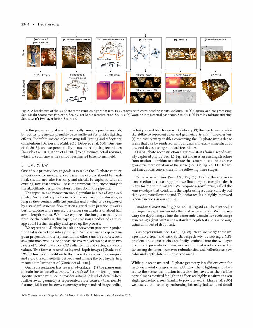
Fig. 2. A breakdown of the 3D photo reconstruction algorithm into its six stages, with corresponding inputs and outputs: (a) Capture and pre-processing,Sec. 4.1; (b) Sparse reconstruction, Sec. 4.2; (c) Dense reconstruction, Sec. 4.3; (d)Warping into a central panorama, Sec. 4.4.1; (e) Parallax-tolerant stitching,Sec. 4.4.2; (f) Two-layer fusion, Sec. 4.4.3.
In this paper, our goal is not to explicitly compute precise normals,
but rather to generate plausible ones, sufficient for artistic lighting
effects. Therefore, instead of estimating full lighting and reflectance
distributions [Barron and Malik 2015; Debevec et al. 2004; Duchêne
et al. 2015], we use perceptually plausible relighting techniques
[Karsch et al. 2011; Khan et al. 2006] to hallucinate detail normals,
which we combine with a smooth estimated base normal field.
3 OVERVIEWOne of our primary design goals is to make the 3D photo capture
process easy for inexperienced users: the capture should be hand-
held, should not take too long, and should be captured with an
existing, low-cost camera. These requirements influenced many of
the algorithmic design decisions further down the pipeline.
The input to our reconstruction algorithm is a set of captured
photos. We do not require them to be taken in any particular way, as
long as they contain sufficient parallax and overlap to be registered
by a standard structure from motion algorithm. In practice, it works
best to capture while moving the camera on a sphere of about half
arm’s length radius. While we captured the images manually to
produce the results in this paper, we envision a dedicated capture
app could further simplify and speed up the process.
We represent a 3D photo in a single-viewpoint panoramic projec-
tion that is discretized into a pixel grid. While we use an equirectan-
gular projection in our representation, other sensible choices, such
as a cube map, would also be possible. Every pixel can hold up to two
layers of “nodes” that store RGB radiance, normal vector, and depth
values. This format resembles layered depth images [Shade et al.
1998]. However, in addition to the layered nodes, we also compute
and store the connectivity between and among the two layers, in a
manner similar to that of [Zitnick et al. 2004].
Our representation has several advantages: (1) the panoramic
domain has an excellent resolution trade-off for rendering from a
specific viewpoint, since it provides automatic level-of-detail where
further away geometry is represented more coarsely than nearby
features; (2) it can be stored compactly using standard image coding
techniques and tiled for network delivery; (3) the two layers provide
the ability to represent color and geometric details at disocclusions;(4) the connectivity enables converting the 3D photo into a dense
mesh that can be rendered without gaps and easily simplified for
low-end devices using standard techniques.
Our 3D photo reconstruction algorithm starts from a set of casu-
ally captured photos (Sec. 4.1, Fig. 2a) and uses an existing structure
from motion algorithm to estimate the camera poses and a sparse
geometric representation of the scene (Sec. 4.2, Fig. 2b). Our techni-
cal innovations concentrate in the following three stages:
Dense reconstruction (Sec. 4.3 / Fig. 2c). Taking the sparse re-
construction as a starting point, we first compute complete depth
maps for the input images. We propose a novel prior, called the
near envelope, that constrains the depth using a conservatively but
tightly estimated lower bound. This prior results in highly improved
reconstructions in our setting.
Parallax-tolerant stitching (Sec. 4.4.1-2 / Fig. 2d-e). The next goal isto merge the depth images into the final representation. We forward-
warp the depth images into the panoramic domain, for each image
generating a front warp using a standard depth test and a back warpusing an inverted depth test.
Two-Layer Fusion (Sec. 4.4.3 / Fig. 2f). Next, we merge these im-
ages into a front and back stitch, respectively, by solving a MRF
problem. These two stitches are finally combined into the two-layer
3D photo representation using an algorithm that resolves connectiv-
ity among the layers, removes redundancies, and hallucinates new
color and depth data in unobserved areas.
While our reconstructed 3D photo geometry is sufficient even for
large viewpoint changes, when adding synthetic lighting and shad-
ing to the scene, the illusion is quickly destroyed, as the surface
normal maps required for lighting effects are highly sensitive to even
slight geometric errors. Similar to previous work [Khan et al. 2006]
we resolve this issue by embossing intensity-hallucinated detail
ACM Transactions on Graphics, Vol. 36, No. 6, Article 234. Publication date: November 2017.
Casual 3D Photography • 234:5
onto a coarse base normal map derived from smoothing the stitched
geometry. The resulting normal map is not real but it contains plau-sible normals that enable artist-driven lighting effects (full-blown
relighting is beyond the scope of this paper).
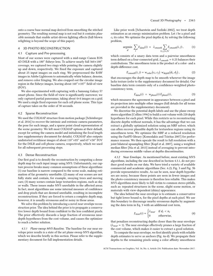
4 3D PHOTO RECONSTRUCTION4.1 Capture and Pre-processingMost of our scenes were captured with a mid-range Canon EOS
6D DSLR with a 180◦fisheye lens. To achieve nearly full 360×180◦
coverage, we captured two rings while pointing the camera slightly
up and down, respectively. We fixed the exposure and captured
about 25 input images on each ring. We preprocessed the RAW
images in Adobe Lightroom to automatically white balance, denoise,
and remove color fringing. We also cropped out the circular image
region in the fisheye images, leaving about 160◦×107◦ field-of-view
(FOV).
We also experimented with capturing with a Samsung Galaxy S7
smart phone. Since the field-of-view is significantly narrower, we
only captured partial panoramas, taking about 4×4 images on a grid.
We used a single fixed exposure for each cell phone scene. This type
of capture takes on the order of 30 seconds.
4.2 Sparse ReconstructionWe used the COLMAP structure from motion package [Schönberger
et al. 2016] to recover the intrinsic and extrinsic camera parameters,
the pose for each image, and a sparse point cloud representation of
the scene geometry. We left most COLMAP options at their default,
except for setting the camera model and initializing the focal length
(see supplementary document for details). COLMAP also outputs
undistorted rectilinear images of about 110◦×85◦ and 65◦×50◦ FOV
for the DSLR and cell phone camera, respectively, which we used
for all subsequent processing steps.
4.3 Dense ReconstructionOur first goal is to densify the reconstruction by computing a dense
depth map for each input image using MVS. Unfortunately, our cap-
ture process breaks many common assumptions of these algorithms:
(1) our baseline is narrow compared to the scene scale, making esti-
mation of far geometry unreliable; (2) many of our scenes are not
fully static and contain, for example, swaying trees and moving
cars; (3) many scenes contain large textureless regions, such as sky
or walls. These issues make MVS unreliable in the affected areas.
In fact, most algorithms use some internal measure of confidence
and drop pixels that are deemed unreliable, resulting in incomplete
reconstructions. If they are forced to return a complete depth map,
however, it is usually erroneous and/or noisy in those areas.
We solve this problem by introducing a novel near envelope recon-struction prior. The idea behind the prior is to propagate a conserva-
tive lower depth bound from confident to the less confident pixels.
The prior effectively discards a large fraction of erroneous near-
depth hypotheses from the cost volume, and causes the optimizer
to reach a better solution.
4.3.1 Plane-sweep MVS Baseline. The baseline for our near en-velope prior results is a state of the art plane-sweep MVS algorithm,
which we describe briefly in this section. Please refer to the supple-
mentary document for full implementation details.
Like prior work [Scharstein and Szeliski 2002], we treat depth
estimation as an energy minimization problem. Let i be a pixel andci its color. We optimize the pixel depths di by solving the followingproblem,
argmin
d
∑iEdata(i) + λsmooth
∑(i, j)∈𝒩
Esmooth(i, j) , (1)
which consists of a unary data term and a pairwise smoothness
term defined on a four-connected grid, λsmooth = 0.25 balances theircontributions. The smoothness term is the product of a color- and a
depth-difference cost,
Esmooth(i, j) = wcolor(ci , c j
)wdepth
(di ,dj
), (2)
that encourages the depth map to be smooth wherever the image
lacks texture (refer to the supplementary document for details). Our
baseline data term consists only of a confidence-weighted photo-
consistency term,
Edata(i) = wphoto(i)Ephoto(i) , (3)
which measures the agreement in appearance between a pixel and
its projection into multiple other images (full details for all terms
are provided in the supplementary document).
We discretize the potential depth labels and use the plane-sweep
stereo algorithm [Collins 1996] to build a cost volumewith 220 depth
hypotheses for each pixel. While this restricts us to reconstructing
discrete depths without normals, it has the advantage that we can
extract a globally optimized solution using an MRF solver, which
can often recover plausible depth for textureless regions using its
smoothness term. We optimize the MRF at a reduced resolution
using the FastPD library [Komodakis and Tziritas 2007] for perfor-
mance reasons. We then upscale the result to full resolution with a
joint bilateral upsampling filter [Kopf et al. 2007], using a weighted
median filter [Ma et al. 2013] instead of averaging to prevent intro-
ducing erroneous middle values at depths discontinuities.
4.3.2 Near Envelope. As mentioned before, most existing MVS
algorithms, including the one described in Section 4.3.1, do not pro-
duce good results on our data. We have tried a variety of available
commercial and academic algorithms (Sec. 6.2); Fig. 3 and Fig. 5b
provide representative results. As can be seen, near-depth hypothe-
ses are noisy, because these points are seen in fewer images and
the photo-consistency measure is therefore less reliable. This makes
MVS algorithms more likely to fall victim to common stereo pitfalls,
such as: repeated structures in the scene, slight scene motion, or
materials with view-dependent (shiny) appearance.
The idea behind the near envelope is to estimate a conservative
but tight lower bound ni for the pixel depths at each pixel. We use
this boundary to discourage nearby erroneous depths by augment-
ing the data term in Eq. 3 with an additional cost term,
Enear(i) =
{λnear if di < ni
0 otherwise,
(4)
that penalizes reconstructing depths closer than the near envelope
(λnear = 1). The near envelope effectively prunes a large fraction of
the cost volume, which makes it easier to extract a good solution.
To compute the near envelope, we first identify pixels with reliable
depth estimates to serve as anchors (Fig. 4a-d). We propagate their
depths to the remaining pixels using a color affinity smoothness
ACM Transactions on Graphics, Vol. 36, No. 6, Article 234. Publication date: November 2017.
234:6 • Hedman et. al.
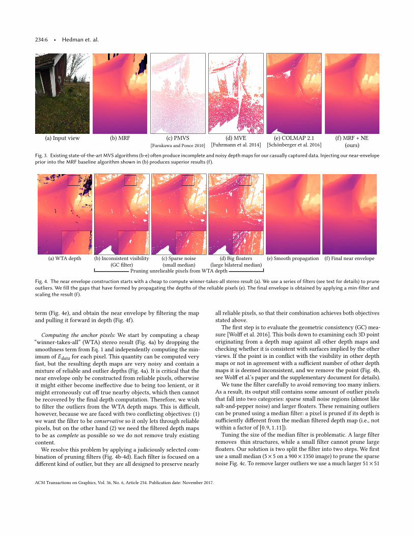
(a) Input view (b) MRF (c) PMVS
[Furukawa and Ponce 2010]
(d) MVE
[Fuhrmann et al. 2014]
(e) COLMAP 2.1
[Schönberger et al. 2016]
(f) MRF + NE
(ours)
Fig. 3. Existing state-of-the-artMVS algorithms (b-e) often produce incomplete and noisy depthmaps for our casually captured data. Injecting our near-envelopeprior into the MRF baseline algorithm shown in (b) produces superior results (f).
(a) WTA depth (b) Inconsistent visibility
(GC filter)
(c) Sparse noise
(small median)
(d) Big floaters
(large bilateral median)
Pruning unrelieable pixels from WTA depth
(e) Smooth propagation (f) Final near envelope
Fig. 4. The near envelope construction starts with a cheap to compute winner-takes-all stereo result (a). We use a series of filters (see text for details) to pruneoutliers. We fill the gaps that have formed by propagating the depths of the reliable pixels (e). The final envelope is obtained by applying a min-filter andscaling the result (f).
term (Fig. 4e), and obtain the near envelope by filtering the map
and pulling it forward in depth (Fig. 4f).
Computing the anchor pixels: We start by computing a cheap
“winner-takes-all” (WTA) stereo result (Fig. 4a) by dropping the
smoothness term from Eq. 1 and independently computing the min-
imum of Edata for each pixel. This quantity can be computed very
fast, but the resulting depth maps are very noisy and contain a
mixture of reliable and outlier depths (Fig. 4a). It is critical that the
near envelope only be constructed from reliable pixels, otherwise
it might either become ineffective due to being too lenient, or it
might erroneously cut off true nearby objects, which then cannot
be recovered by the final depth computation. Therefore, we wish
to filter the outliers from the WTA depth maps. This is difficult,
however, because we are faced with two conflicting objectives: (1)
we want the filter to be conservative so it only lets through reliable
pixels, but on the other hand (2) we need the filtered depth maps
to be as complete as possible so we do not remove truly existing
content.
We resolve this problem by applying a judiciously selected com-
bination of pruning filters (Fig. 4b-4d). Each filter is focused on a
different kind of outlier, but they are all designed to preserve nearly
all reliable pixels, so that their combination achieves both objectives
stated above.
The first step is to evaluate the geometric consistency (GC) mea-
sure [Wolff et al. 2016]. This boils down to examining each 3D point
originating from a depth map against all other depth maps and
checking whether it is consistent with surfaces implied by the other
views. If the point is in conflict with the visibility in other depth
maps or not in agreement with a sufficient number of other depth
maps it is deemed inconsistent, and we remove the point (Fig. 4b,
see Wolff et al.’s paper and the supplementary document for details).
We tune the filter carefully to avoid removing too many inliers.
As a result, its output still contains some amount of outlier pixels
that fall into two categories: sparse small noise regions (almost like
salt-and-pepper noise) and larger floaters. These remaining outliers
can be pruned using a median filter: a pixel is pruned if its depth is
sufficiently different from the median filtered depth map (i.e., not
within a factor of [0.9, 1.11]).Tuning the size of the median filter is problematic. A large filter
removes thin structures, while a small filter cannot prune large
floaters. Our solution is two split the filter into two steps. We first
use a small median (5× 5 on a 900× 1350 image) to prune the sparse
noise Fig. 4c. To remove larger outliers we use a much larger 51× 51
ACM Transactions on Graphics, Vol. 36, No. 6, Article 234. Publication date: November 2017.
Casual 3D Photography • 234:7
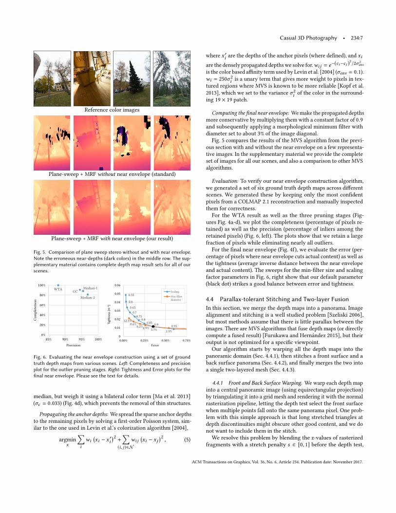
Reference color images
Plane-sweep + MRF without near envelope (standard)
Plane-sweep + MRF with near envelope (our result)
Fig. 5. Comparison of plane sweep stereo without and with near envelope.Note the erroneous near-depths (dark colors) in the middle row. The sup-plementary material contains complete depth map result sets for all of ourscenes.
Tigh
tnes
s [m
-1]
Fig. 6. Evaluating the near envelope construction using a set of groundtruth depth maps from various scenes. Left: Completeness and precisionplot for the outlier pruning stages. Right: Tightness and Error plots for thefinal near envelope. Please see the text for details.
median, but weigh it using a bilateral color term [Ma et al. 2013]
(σc = 0.033) (Fig. 4d), which prevents the removal of thin structures.
Propagating the anchor depths: We spread the sparse anchor depths
to the remaining pixels by solving a first-order Poisson system, sim-
ilar to the one used in Levin et al.’s colorization algorithm [2004],
argmin
x
∑iwi
(xi − x ′i
)2
+∑
(i, j)∈𝒩wi j
(xi − x j
)2
, (5)
where x ′i are the depths of the anchor pixels (where defined), and xi
are the densely propagated depthswe solve for.wi j = e−(ci−c j )2
/2σ 2
env
is the color based affinity term used by Levin et al. [2004] (σenv = 0.1).wi = 250σ 2
i is a unary term that gives more weight to pixels in tex-
tured regions where MVS is known to be more reliable [Kopf et al.
2013], which we set to the variance σ 2
i of the color in the surround-
ing 19 × 19 patch.
Computing the final near envelope: Wemake the propagated depths
more conservative by multiplying them with a constant factor of 0.9and subsequently applying a morphological minimum filter with
diameter set to about 3% of the image diagonal.
Fig. 5 compares the results of the MVS algorithm from the previ-
ous section with and without the near envelope on a few representa-
tive images. In the supplementary material we provide the complete
set of images for all our scenes, and also a comparison to other MVS
algorithms.
Evaluation: To verify our near envelope construction algorithm,
we generated a set of six ground truth depth maps across different
scenes. We generated these by keeping only the most confident
pixels from a COLMAP 2.1 reconstruction and manually inspected
them for correctness.
For the WTA result as well as the three pruning stages (Fig-
ures Fig. 4a-d), we plot the completeness (percentage of pixels re-
tained) as well as the precision (percentage of inliers among the
retained pixels) (Fig. 6, left). The plots show that we retain a large
fraction of pixels while eliminating nearly all outliers.
For the final near envelope (Fig. 4f), we evaluate the error (per-
centage of pixels where near envelope cuts actual content) as well as
the tightness (average inverse distance between the near envelope
and actual content). The sweeps for the min-filter size and scaling
factor parameters in Fig. 6, right show that our default parameter
(black dot) strikes a good balance between error and tightness.
4.4 Parallax-tolerant Stitching and Two-layer FusionIn this section, we merge the depth maps into a panorama. Image
alignment and stitching is a well studied problem [Szeliski 2006],
but most methods assume that there is little parallax between the
images. There are MVS algorithms that fuse depth maps (or directly
compute a fused result) [Furukawa and Hernández 2015], but their
output is not optimized for a specific viewpoint.
Our algorithm starts by warping all the depth maps into the
panoramic domain (Sec. 4.4.1), then stitches a front surface and a
back surface panorama (Sec. 4.4.2), and finally merges the two into
a single two-layered mesh (Sec. 4.4.3).
4.4.1 Front and Back Surface Warping. We warp each depth map
into a central panoramic image (using equirectangular projection)
by triangulating it into a grid mesh and rendering it with the normal
rasterization pipeline, letting the depth test select the front surface
when multiple points fall onto the same panorama pixel. One prob-
lem with this simple approach is that long stretched triangles at
depth discontinuities might obscure other good content, and we do
not want to include them in the stitch.
We resolve this problem by blending the z-values of rasterized
fragments with a stretch penalty s ∈ [0, 1] before the depth test,
ACM Transactions on Graphics, Vol. 36, No. 6, Article 234. Publication date: November 2017.
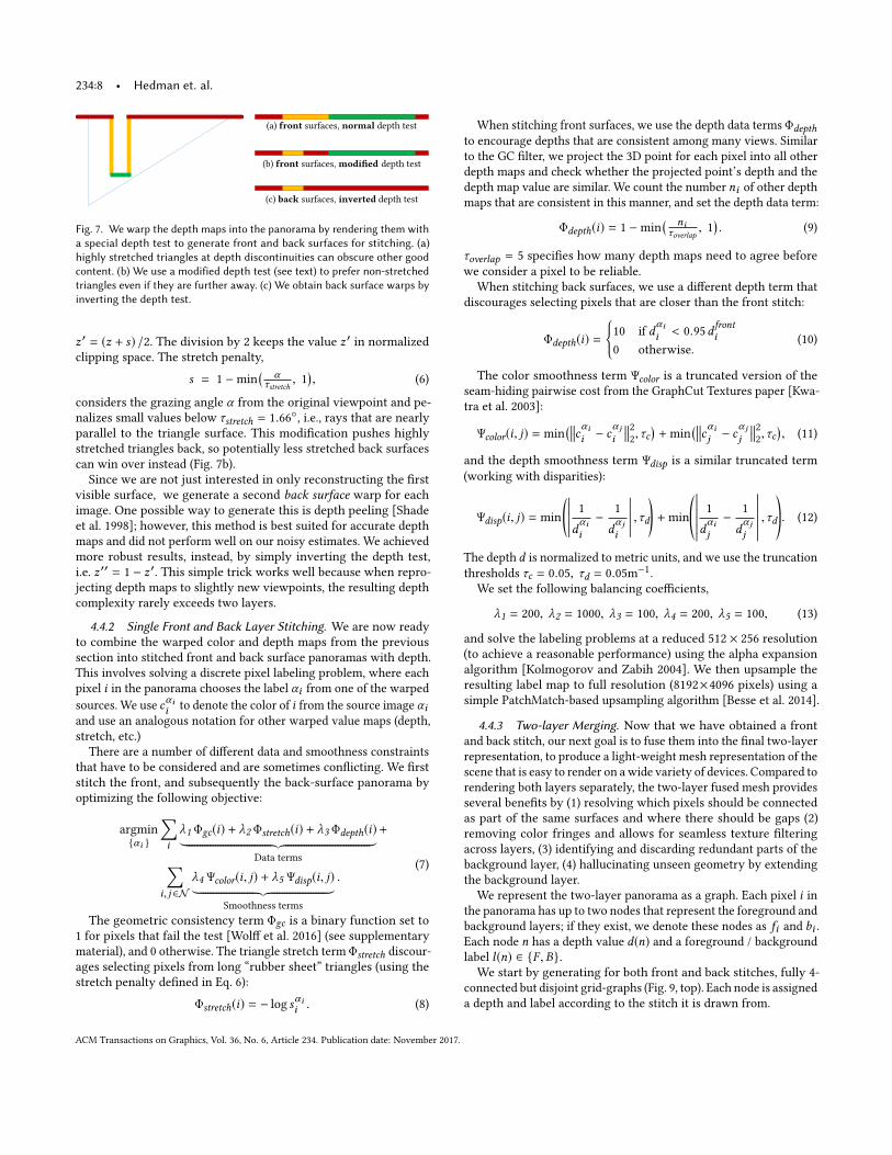
234:8 • Hedman et. al.
back inverted
front modified
front normal
Fig. 7. We warp the depth maps into the panorama by rendering them witha special depth test to generate front and back surfaces for stitching. (a)highly stretched triangles at depth discontinuities can obscure other goodcontent. (b) We use a modified depth test (see text) to prefer non-stretchedtriangles even if they are further away. (c) We obtain back surface warps byinverting the depth test.
z′ = (z + s) /2. The division by 2 keeps the value z′ in normalized
clipping space. The stretch penalty,
s = 1 −min
( ατstretch , 1
), (6)
considers the grazing angle α from the original viewpoint and pe-
nalizes small values below τstretch = 1.66◦, i.e., rays that are nearlyparallel to the triangle surface. This modification pushes highly
stretched triangles back, so potentially less stretched back surfaces
can win over instead (Fig. 7b).
Since we are not just interested in only reconstructing the first
visible surface, we generate a second back surface warp for each
image. One possible way to generate this is depth peeling [Shade
et al. 1998]; however, this method is best suited for accurate depth
maps and did not perform well on our noisy estimates. We achieved
more robust results, instead, by simply inverting the depth test,
i.e. z′′ = 1 − z′. This simple trick works well because when repro-
jecting depth maps to slightly new viewpoints, the resulting depth
complexity rarely exceeds two layers.
4.4.2 Single Front and Back Layer Stitching. We are now ready
to combine the warped color and depth maps from the previous
section into stitched front and back surface panoramas with depth.
This involves solving a discrete pixel labeling problem, where each
pixel i in the panorama chooses the label αi from one of the warped
sources. We use cαii to denote the color of i from the source image αiand use an analogous notation for other warped value maps (depth,
stretch, etc.)
There are a number of different data and smoothness constraints
that have to be considered and are sometimes conflicting. We first
stitch the front, and subsequently the back-surface panorama by
optimizing the following objective:
argmin
{αi }
∑iλ1 Φgc(i) + λ2 Φstretch(i) + λ3 Φdepth(i)︸ ︷︷ ︸
Data terms
+
∑i, j ∈𝒩
λ4 Ψcolor(i, j) + λ5 Ψdisp(i, j)︸ ︷︷ ︸Smoothness terms
.(7)
The geometric consistency term Φgc is a binary function set to
1 for pixels that fail the test [Wolff et al. 2016] (see supplementary
material), and 0 otherwise. The triangle stretch term Φstretch discour-ages selecting pixels from long “rubber sheet” triangles (using the
stretch penalty defined in Eq. 6):
Φstretch(i) = − log sαii . (8)
When stitching front surfaces, we use the depth data terms Φdepthto encourage depths that are consistent among many views. Similar
to the GC filter, we project the 3D point for each pixel into all other
depth maps and check whether the projected point’s depth and the
depth map value are similar. We count the number ni of other depthmaps that are consistent in this manner, and set the depth data term:
Φdepth(i) = 1 −min
( niτoverlap , 1
). (9)
τoverlap = 5 specifies how many depth maps need to agree before
we consider a pixel to be reliable.
When stitching back surfaces, we use a different depth term that
discourages selecting pixels that are closer than the front stitch:
Φdepth(i) =
{10 if d
αii < 0.95d
fronti
0 otherwise.
(10)
The color smoothness term Ψcolor is a truncated version of the
seam-hiding pairwise cost from the GraphCut Textures paper [Kwa-
tra et al. 2003]:
Ψcolor(i, j) = min
( cαii − cα ji
22,τc
)+min
( cαij − cα jj
22,τc
), (11)
and the depth smoothness term Ψdisp is a similar truncated term
(working with disparities):
Ψdisp(i, j) = min
(����� 1
dαii
−1
dα ji
����� ,τd)+min
©«������ 1
dαij
−1
dα jj
������ ,τdª®¬. (12)
The depth d is normalized to metric units, and we use the truncation
thresholds τc = 0.05, τd = 0.05m−1.
We set the following balancing coefficients,
λ1 = 200, λ2 = 1000, λ3 = 100, λ4 = 200, λ5 = 100, (13)
and solve the labeling problems at a reduced 512 × 256 resolution
(to achieve a reasonable performance) using the alpha expansion
algorithm [Kolmogorov and Zabih 2004]. We then upsample the
resulting label map to full resolution (8192×4096 pixels) using a
simple PatchMatch-based upsampling algorithm [Besse et al. 2014].
4.4.3 Two-layer Merging. Now that we have obtained a front
and back stitch, our next goal is to fuse them into the final two-layer
representation, to produce a light-weight mesh representation of the
scene that is easy to render on awide variety of devices. Compared to
rendering both layers separately, the two-layer fused mesh provides
several benefits by (1) resolving which pixels should be connected
as part of the same surfaces and where there should be gaps (2)
removing color fringes and allows for seamless texture filtering
across layers, (3) identifying and discarding redundant parts of the
background layer, (4) hallucinating unseen geometry by extending
the background layer.
We represent the two-layer panorama as a graph. Each pixel i inthe panorama has up to two nodes that represent the foreground and
background layers; if they exist, we denote these nodes as fi and bi .Each node n has a depth value d(n) and a foreground / background
label l(n) ∈ {F ,B}.We start by generating for both front and back stitches, fully 4-
connected but disjoint grid-graphs (Fig. 9, top). Each node is assigned
a depth and label according to the stitch it is drawn from.
ACM Transactions on Graphics, Vol. 36, No. 6, Article 234. Publication date: November 2017.
Casual 3D Photography • 234:9
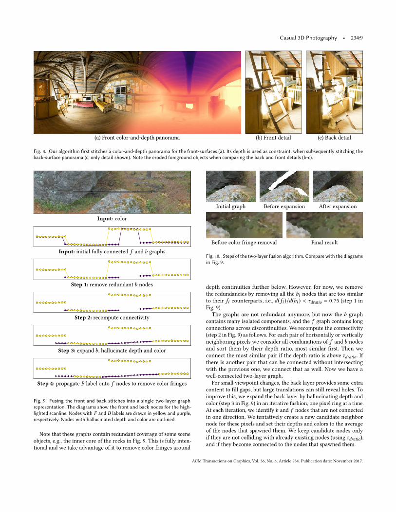
(a) Front color-and-depth panorama (b) Front detail (c) Back detail
Fig. 8. Our algorithm first stitches a color-and-depth panorama for the front-surfaces (a). Its depth is used as constraint, when subsequently stitching theback-surface panorama (c, only detail shown). Note the eroded foreground objects when comparing the back and front details (b-c).
Input: color
Input: initial fully connected f and b graphs
Step 1: remove redundant b nodes
Step 2: recompute connectivity
Step 3: expand b, hallucinate depth and color
Step 4: propagate B label onto f nodes to remove color fringes
Fig. 9. Fusing the front and back stitches into a single two-layer graphrepresentation. The diagrams show the front and back nodes for the high-lighted scanline. Nodes with F and B labels are drawn in yellow and purple,respectively. Nodes with hallucinated depth and color are outlined.
Note that these graphs contain redundant coverage of some scene
objects, e.g., the inner core of the rocks in Fig. 9. This is fully inten-
tional and we take advantage of it to remove color fringes around
Initial graph Before expansion After expansion
Before color fringe removal Final result
Fig. 10. Steps of the two-layer fusion algorithm. Compare with the diagramsin Fig. 9.
depth continuities further below. However, for now, we remove
the redundancies by removing all the bi nodes that are too similar
to their fi counterparts, i.e., d(fi )/d(bi ) < τdratio = 0.75 (step 1 in
Fig. 9).
The graphs are not redundant anymore, but now the b graph
contains many isolated components, and the f graph contains long
connections across discontinuities. We recompute the connectivity
(step 2 in Fig. 9) as follows. For each pair of horizontally or vertically
neighboring pixels we consider all combinations of f and b nodes
and sort them by their depth ratio, most similar first. Then we
connect the most similar pair if the depth ratio is above τdratio. Ifthere is another pair that can be connected without intersecting
with the previous one, we connect that as well. Now we have a
well-connected two-layer graph.
For small viewpoint changes, the back layer provides some extra
content to fill gaps, but large translations can still reveal holes. To
improve this, we expand the back layer by hallucinating depth and
color (step 3 in Fig. 9) in an iterative fashion, one pixel ring at a time.
At each iteration, we identify b and f nodes that are not connected
in one direction. We tentatively create a new candidate neighbor
node for these pixels and set their depths and colors to the average
of the nodes that spawned them. We keep candidate nodes only
if they are not colliding with already existing nodes (using τdratio),and if they become connected to the nodes that spawned them.
ACM Transactions on Graphics, Vol. 36, No. 6, Article 234. Publication date: November 2017.
234:10 • Hedman et. al.
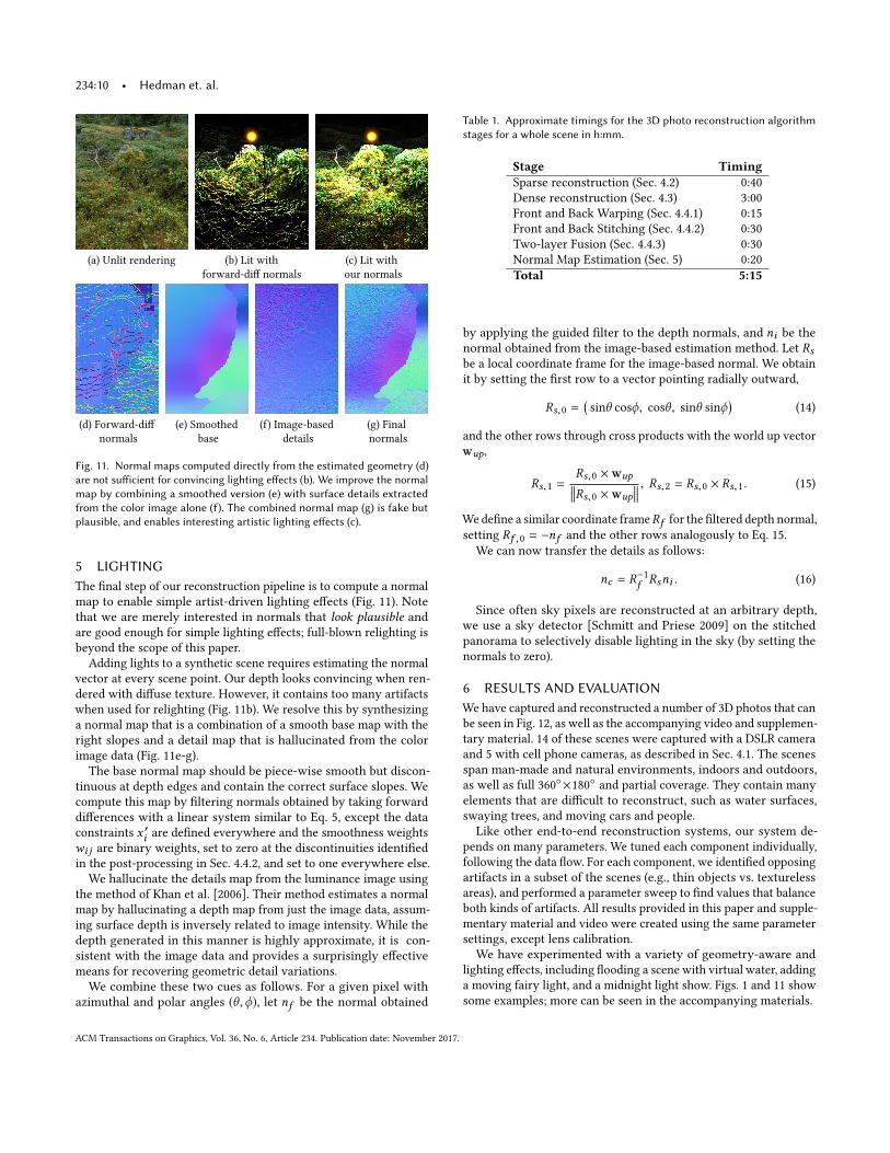
(a) Unlit rendering (b) Lit with
forward-diff normals
(c) Lit with
our normals
(d) Forward-diff
normals
(e) Smoothed
base
(f) Image-based
details
(g) Final
normals
Fig. 11. Normal maps computed directly from the estimated geometry (d)are not sufficient for convincing lighting effects (b). We improve the normalmap by combining a smoothed version (e) with surface details extractedfrom the color image alone (f). The combined normal map (g) is fake butplausible, and enables interesting artistic lighting effects (c).
5 LIGHTINGThe final step of our reconstruction pipeline is to compute a normal
map to enable simple artist-driven lighting effects (Fig. 11). Note
that we are merely interested in normals that look plausible andare good enough for simple lighting effects; full-blown relighting is
beyond the scope of this paper.
Adding lights to a synthetic scene requires estimating the normal
vector at every scene point. Our depth looks convincing when ren-
dered with diffuse texture. However, it contains too many artifacts
when used for relighting (Fig. 11b). We resolve this by synthesizing
a normal map that is a combination of a smooth base map with the
right slopes and a detail map that is hallucinated from the color
image data (Fig. 11e-g).
The base normal map should be piece-wise smooth but discon-
tinuous at depth edges and contain the correct surface slopes. We
compute this map by filtering normals obtained by taking forward
differences with a linear system similar to Eq. 5, except the data
constraints x ′i are defined everywhere and the smoothness weights
wi j are binary weights, set to zero at the discontinuities identified
in the post-processing in Sec. 4.4.2, and set to one everywhere else.
We hallucinate the details map from the luminance image using
the method of Khan et al. [2006]. Their method estimates a normal
map by hallucinating a depth map from just the image data, assum-
ing surface depth is inversely related to image intensity. While the
depth generated in this manner is highly approximate, it is con-
sistent with the image data and provides a surprisingly effective
means for recovering geometric detail variations.
We combine these two cues as follows. For a given pixel with
azimuthal and polar angles (θ ,ϕ), let nf be the normal obtained
Table 1. Approximate timings for the 3D photo reconstruction algorithmstages for a whole scene in h:mm.
Stage TimingSparse reconstruction (Sec. 4.2) 0:40
Dense reconstruction (Sec. 4.3) 3:00
Front and Back Warping (Sec. 4.4.1) 0:15
Front and Back Stitching (Sec. 4.4.2) 0:30
Two-layer Fusion (Sec. 4.4.3) 0:30
Normal Map Estimation (Sec. 5) 0:20
Total 5:15
by applying the guided filter to the depth normals, and ni be thenormal obtained from the image-based estimation method. Let Rsbe a local coordinate frame for the image-based normal. We obtain
it by setting the first row to a vector pointing radially outward,
Rs,0 =(sinθ cosϕ, cosθ , sinθ sinϕ
)(14)
and the other rows through cross products with the world up vector
wup,
Rs,1 =Rs,0 ×wup Rs,0 ×wup
, Rs,2 = Rs,0 × Rs,1. (15)
We define a similar coordinate frameRf for the filtered depth normal,
setting Rf ,0 = −nf and the other rows analogously to Eq. 15.
We can now transfer the details as follows:
nc = R−1f Rsni . (16)
Since often sky pixels are reconstructed at an arbitrary depth,
we use a sky detector [Schmitt and Priese 2009] on the stitched
panorama to selectively disable lighting in the sky (by setting the
normals to zero).
6 RESULTS AND EVALUATIONWe have captured and reconstructed a number of 3D photos that can
be seen in Fig. 12, as well as the accompanying video and supplemen-
tary material. 14 of these scenes were captured with a DSLR camera
and 5 with cell phone cameras, as described in Sec. 4.1. The scenes
span man-made and natural environments, indoors and outdoors,
as well as full 360◦×180◦ and partial coverage. They contain many
elements that are difficult to reconstruct, such as water surfaces,
swaying trees, and moving cars and people.
Like other end-to-end reconstruction systems, our system de-
pends on many parameters. We tuned each component individually,
following the data flow. For each component, we identified opposing
artifacts in a subset of the scenes (e.g., thin objects vs. textureless
areas), and performed a parameter sweep to find values that balance
both kinds of artifacts. All results provided in this paper and supple-
mentary material and video were created using the same parameter
settings, except lens calibration.
We have experimented with a variety of geometry-aware and
lighting effects, including flooding a scene with virtual water, adding
a moving fairy light, and a midnight light show. Figs. 1 and 11 show
some examples; more can be seen in the accompanying materials.
ACM Transactions on Graphics, Vol. 36, No. 6, Article 234. Publication date: November 2017.
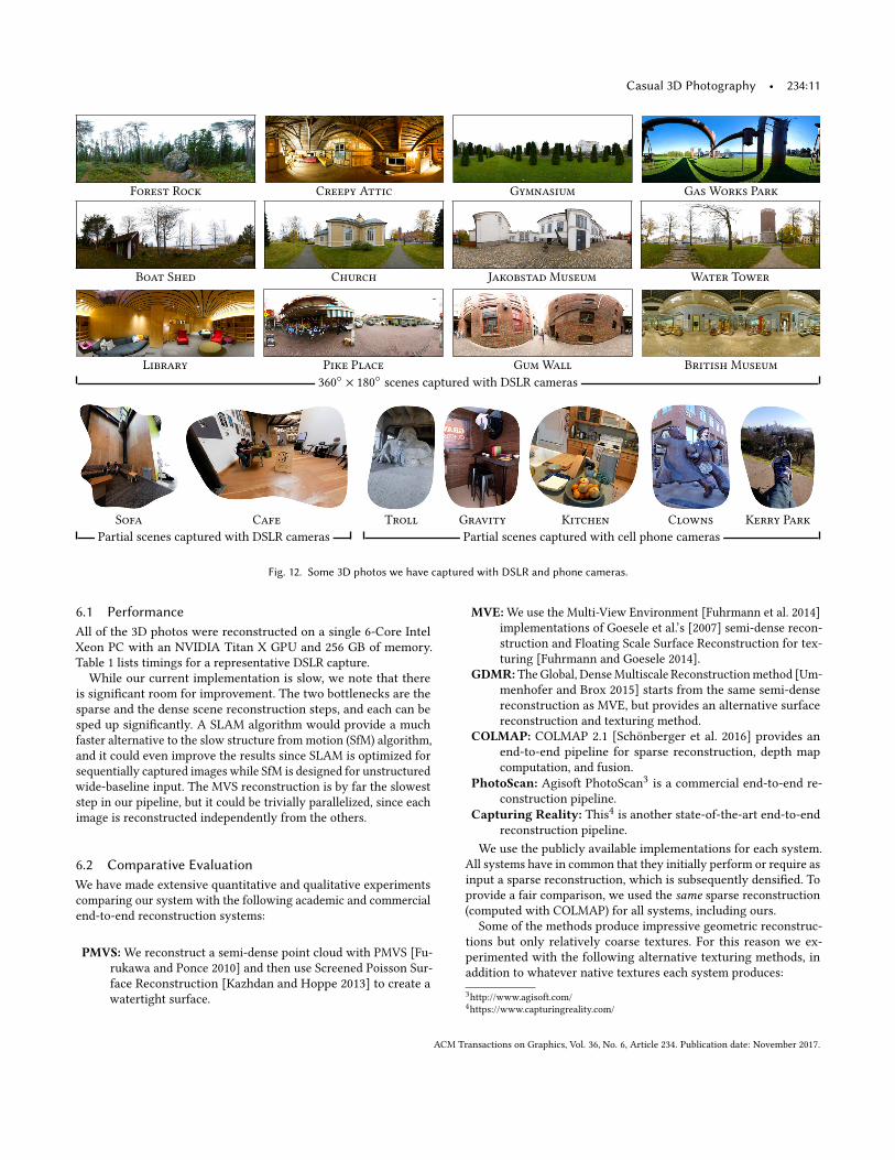
Casual 3D Photography • 234:11
Forest Rock Creepy Attic Gymnasium Gas Works Park
Boat Shed Church Jakobstad Museum Water Tower
Library Pike Place Gum Wall British Museum
360◦ × 180
◦scenes captured with DSLR cameras
Sofa Cafe
Partial scenes captured with DSLR cameras
Troll Gravity Kitchen Clowns Kerry Park
Partial scenes captured with cell phone cameras
Fig. 12. Some 3D photos we have captured with DSLR and phone cameras.
6.1 PerformanceAll of the 3D photos were reconstructed on a single 6-Core Intel
Xeon PC with an NVIDIA Titan X GPU and 256 GB of memory.
Table 1 lists timings for a representative DSLR capture.
While our current implementation is slow, we note that there
is significant room for improvement. The two bottlenecks are the
sparse and the dense scene reconstruction steps, and each can be
sped up significantly. A SLAM algorithm would provide a much
faster alternative to the slow structure from motion (SfM) algorithm,
and it could even improve the results since SLAM is optimized for
sequentially captured images while SfM is designed for unstructured
wide-baseline input. The MVS reconstruction is by far the slowest
step in our pipeline, but it could be trivially parallelized, since each
image is reconstructed independently from the others.
6.2 Comparative EvaluationWe have made extensive quantitative and qualitative experiments
comparing our system with the following academic and commercial
end-to-end reconstruction systems:
PMVS:We reconstruct a semi-dense point cloud with PMVS [Fu-
rukawa and Ponce 2010] and then use Screened Poisson Sur-
face Reconstruction [Kazhdan and Hoppe 2013] to create a
watertight surface.
MVE:We use the Multi-View Environment [Fuhrmann et al. 2014]
implementations of Goesele et al.’s [2007] semi-dense recon-
struction and Floating Scale Surface Reconstruction for tex-
turing [Fuhrmann and Goesele 2014].
GDMR:TheGlobal, DenseMultiscale Reconstructionmethod [Um-
menhofer and Brox 2015] starts from the same semi-dense
reconstruction as MVE, but provides an alternative surface
reconstruction and texturing method.
COLMAP: COLMAP 2.1 [Schönberger et al. 2016] provides an
end-to-end pipeline for sparse reconstruction, depth map
computation, and fusion.
PhotoScan: Agisoft PhotoScan3 is a commercial end-to-end re-
construction pipeline.
Capturing Reality: This4 is another state-of-the-art end-to-endreconstruction pipeline.
We use the publicly available implementations for each system.
All systems have in common that they initially perform or require as
input a sparse reconstruction, which is subsequently densified. To
provide a fair comparison, we used the same sparse reconstruction(computed with COLMAP) for all systems, including ours.
Some of the methods produce impressive geometric reconstruc-
tions but only relatively coarse textures. For this reason we ex-
perimented with the following alternative texturing methods, in
addition to whatever native textures each system produces:
3http://www.agisoft.com/
4https://www.capturingreality.com/
ACM Transactions on Graphics, Vol. 36, No. 6, Article 234. Publication date: November 2017.
234:12 • Hedman et. al.
0
0.02
0.04
0.06
0.08
0.1
0.12
SADError
Samples[%]
Native Textures TexRecon Textures [Waechter et al. 2014] Unstructured Lumigraph [Buehler et al. 2001]
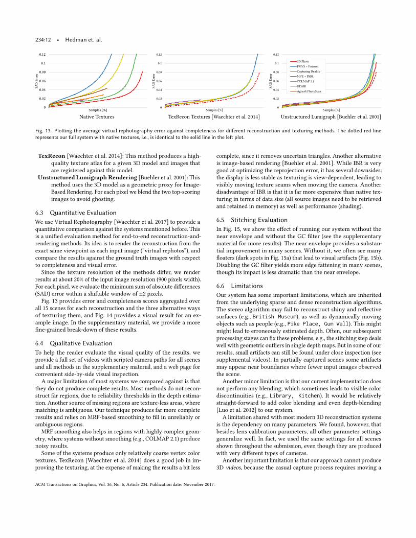
Fig. 13. Plotting the average virtual rephotography error against completeness for different reconstruction and texturing methods. The dotted red linerepresents our full system with native textures, i.e., is identical to the solid line in the left plot.
TexRecon [Waechter et al. 2014]: This method produces a high-
quality texture atlas for a given 3D model and images that
are registered against this model.
Unstructured Lumigraph Rendering [Buehler et al. 2001]: Thismethod uses the 3D model as a geometric proxy for Image-
Based Rendering. For each pixel we blend the two top-scoring
images to avoid ghosting.
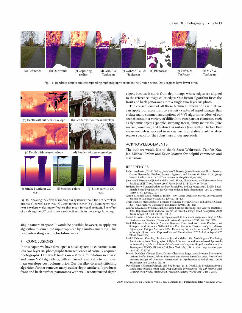
6.3 Quantitative EvaluationWe use Virtual Rephotography [Waechter et al. 2017] to provide a
quantitative comparison against the systems mentioned before. This
is a unified evaluation method for end-to-end reconstruction-and-
rendering methods. Its idea is to render the reconstruction from the
exact same viewpoint as each input image (“virtual rephotos”), and
compare the results against the ground truth images with respect
to completeness and visual error.
Since the texture resolution of the methods differ, we render
results at about 20% of the input image resolution (900 pixels width).
For each pixel, we evaluate the minimum sum of absolute differences
(SAD) error within a shiftable window of ±2 pixels.
Fig. 13 provides error and completeness scores aggregated over
all 15 scenes for each reconstruction and the three alternative ways
of texturing them, and Fig. 14 provides a visual result for an ex-
ample image. In the supplementary material, we provide a more
fine-grained break-down of these results.
6.4 Qualitative EvaluationTo help the reader evaluate the visual quality of the results, we
provide a full set of videos with scripted camera paths for all scenes
and all methods in the supplementary material, and a web page for
convenient side-by-side visual inspection.
A major limitation of most systems we compared against is that
they do not produce complete results. Most methods do not recon-
struct far regions, due to reliability thresholds in the depth estima-
tion. Another source of missing regions are texture-less areas, where
matching is ambiguous. Our technique produces far more complete
results and relies on MRF-based smoothing to fill in unreliably or
ambiguous regions.
MRF smoothing also helps in regions with highly complex geom-
etry, where systems without smoothing (e.g., COLMAP 2.1) produce
noisy results.
Some of the systems produce only relatively coarse vertex color
textures. TexRecon [Waechter et al. 2014] does a good job in im-
proving the texturing, at the expense of making the results a bit less
complete, since it removes uncertain triangles. Another alternative
is image-based rendering [Buehler et al. 2001]. While IBR is very
good at optimizing the reprojection error, it has several downsides:
the display is less stable as texturing is view-dependent, leading to
visibly moving texture seams when moving the camera. Another
disadvantage of IBR is that it is far more expensive than native tex-
turing in terms of data size (all source images need to be retrieved
and retained in memory) as well as performance (shading).
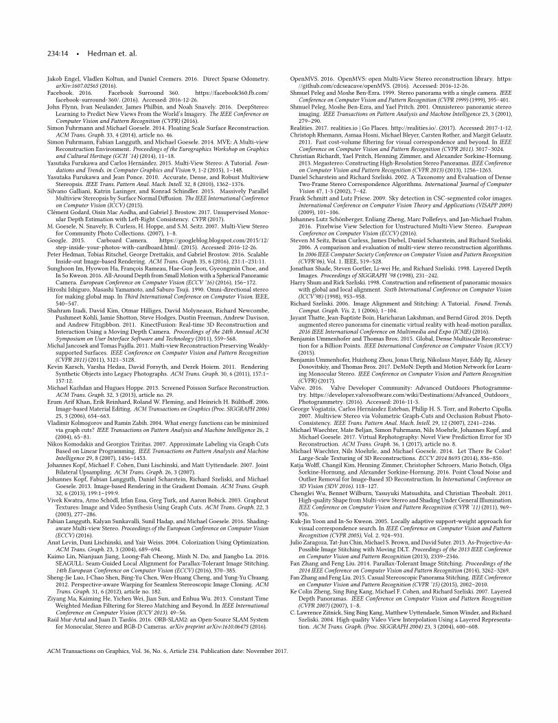
6.5 Stitching EvaluationIn Fig. 15, we show the effect of running our system without the
near envelope and without the GC filter (see the supplementary
material for more results). The near envelope provides a substan-
tial improvement in many scenes. Without it, we often see many
floaters (dark spots in Fig. 15a) that lead to visual artifacts (Fig. 15b).
Disabling the GC filter yields more edge fattening in many scenes,
though its impact is less dramatic than the near envelope.
6.6 LimitationsOur system has some important limitations, which are inherited
from the underlying sparse and dense reconstruction algorithms.
The stereo algorithm may fail to reconstruct shiny and reflective
surfaces (e.g., British Museum), as well as dynamically moving
objects such as people (e.g., Pike Place, Gum Wall). This might
might lead to erroneously estimated depth. Often, our subsequent
processing stages can fix these problems, e.g., the stitching step deals
well with geometric outliers in single depth maps. But in some of our
results, small artifacts can still be found under close inspection (see
supplemental videos). In partially captured scenes some artifacts
may appear near boundaries where fewer input images observed
the scene.
Another minor limitation is that our current implementation does
not perform any blending, which sometimes leads to visible color
discontinuities (e.g., Library, Kitchen). It would be relatively
straight-forward to add color blending and even depth-blending
[Luo et al. 2012] to our system.
A limitation shared with most modern 3D reconstruction systems
is the dependency on many parameters. We found, however, that
besides lens calibration parameters, all other parameter settings
generalize well. In fact, we used the same settings for all scenes
shown throughout the submission, even though they are produced
with very different types of cameras.
Another important limitation is that our approach cannot produce
3D videos, because the casual capture process requires moving a
ACM Transactions on Graphics, Vol. 36, No. 6, Article 234. Publication date: November 2017.
Casual 3D Photography • 234:13
(a) Reference (b) Our result (c) Capturing
reality
(d) GDMR &
TexRecon
(e) COLMAP 2.1 &
TexRecon
(f) Photoscan (g) PMVS &
TexRecon
(h) MVE &
TexRecon
Fig. 14. Rendered results and corresponding rephotography errors in the Church scene. Dark regions have lower error.
(a) Depth without near-envelope (b) Render without near envelope
(c) Depth with near-envelope (d) Render with near envelope
(e) Stitched without GC
cost
(f) Stitched colors (g) Stitched with GC
cost
Fig. 15. Showing the effect of running our system without the near envelopeprior (a-d), as well as without GC cost in the stitcher (e-g). Running withoutnear envelope yields many floaters that result in visual artifacts. The effectof disabling the GC cost is more subtle, it results in more edge fattening.
single camera in space. It would be possible, however, to apply our
algorithm to structured input captured by a multi-camera rig. This
is an interesting avenue for future work.
7 CONCLUSIONSIn this paper, we have developed a novel system to construct seam-
less two-layer 3D photographs from sequences of casually acquired
photographs. Our work builds on a strong foundation in sparse
and dense MVS algorithms, with enhanced results due to our novel
near envelope cost volume prior. Our parallax-tolerant stitching
algorithm further removes many outlier depth artifacts. It produces
front and back surface panoramas with well-reconstructed depth
edges, because it starts from depth maps whose edges are aligned
to the reference image color edges. Our fusion algorithm fuses the
front and back panoramas into a single two-layer 3D photo.
The consequence of all these technical innovations is that we
can apply our algorithm to casually captured input images that
violate many common assumptions of MVS algorithms. Most of our
scenes contain a variety of difficult to reconstruct elements, such
as dynamic objects (people, swaying trees), shiny materials (lake
surface, windows), and textureless surfaces (sky, walls). The fact that
we nevertheless succeed in reconstructing relatively artifact-free
scenes speaks for the robustness of our approach.
ACKNOWLEDGEMENTSThe authors would like to thank Scott Wehrwein, Tianfan Xue,
Jan-Michael Frahm and Kevin Matzen for helpful comments and
discussion.
REFERENCESRobert Anderson, David Gallup, Jonathan T. Barron, Janne Kontkanen, Noah Snavely,
Carlos Hernandez Esteban, Sameer Agarwal, and Steven M. Seitz. 2016. Jump:
Virtual Reality Video. ACM Transactions on Graphics 35, 6 (2016).Jonathan T. Barron and Jitendra Malik. 2015. Shape, Illumination, and Reflectance from
Shading. IEEE Trans. Pattern Anal. Mach. Intell. 37, 8 (2015), 1670–1687.Frederic Besse, Carsten Rother, Andrew Fitzgibbon, and Jan Kautz. 2014. PMBP: Patch-
Match Belief Propagation for Correspondence Field Estimation. Int. J. Comput.Vision 110, 1 (2014), 2–13.
Aaron F. Bobick and Stephen S. Intille. 1999. Large Occlusion Stereo. InternationalJournal of Computer Vision 33, 3 (1999), 181–200.
Chris Buehler, Michael Bosse, Leonard McMillan, Steven Gortler, and Michael Cohen.
2001. Unstructured Lumigraph Rendering. (2001), 425–432.
Gaurav Chaurasia, Sylvain Duchene, Olga Sorkine-Hornung, and George Drettakis.
2013. Depth Synthesis and Local Warps for Plausible Image-based Navigation. ACMTrans. Graph. 32, 3 (2013), 30:1–30:12.
Robert T. Collins. 1996. A space-sweep approach to true multi-image matching. In IEEEConference on Computer Vision and Pattern Recognition (CVPR 1996). 358–363.
Paul Debevec, Chris Tchou, Andrew Gardner, Tim Hawkins, Charis Poullis, Jessi
Stumpfel, Andrew Jones, Nathaniel Yun, Per Einarsson, Therese Lundgren, Marcos
Fajardo, and Philippe Martinez. 2004. Estimating Surface Reflectance Properties of
a Complex Scene under Captured Natural Illumination. ICT Technical Report ICTTR 06 2004 (2004).
Paul E. Debevec, Camillo J. Taylor, and Jitendra Malik. 1996. Modeling and Rendering
Architecture from Photographs: A Hybrid Geometry- and Image-based Approach.
In Proceedings of the 23rd Annual Conference on Computer Graphics and InteractiveTechniques (SIGGRAPH ’96). ACM, New York, NY, USA, 11–20. https://doi.org/10.
1145/237170.237191
Sylvain Duchêne, Clement Riant, Gaurav Chaurasia, Jorge Lopez-Moreno, Pierre-Yves
Laffont, Stefan Popov, Adrien Bousseau, and George Drettakis. 2015. Multi-View
Intrinsic Images of Outdoors Scenes with an Application to Relighting. ACMTransactions on Graphics (2015).
David Eigen, Christian Puhrsch, and Rob Fergus. 2014. Depth Map Prediction from a
Single Image Using a Multi-scale Deep Network. Proceedings of the 27th InternationalConference on Neural Information Processing Systems (NIPS) (2014), 2366–2374.
ACM Transactions on Graphics, Vol. 36, No. 6, Article 234. Publication date: November 2017.
234:14 • Hedman et. al.
Jakob Engel, Vladlen Koltun, and Daniel Cremers. 2016. Direct Sparse Odometry.
arXiv:1607.02565 (2016).Facebook. 2016. Facebook Surround 360. https://facebook360.fb.com/
facebook-surround-360/. (2016). Accessed: 2016-12-26.
John Flynn, Ivan Neulander, James Philbin, and Noah Snavely. 2016. DeepStereo:
Learning to Predict New Views From the World’s Imagery. The IEEE Conference onComputer Vision and Pattern Recognition (CVPR) (2016).
Simon Fuhrmann and Michael Goesele. 2014. Floating Scale Surface Reconstruction.
ACM Trans. Graph. 33, 4 (2014), article no. 46.Simon Fuhrmann, Fabian Langguth, and Michael Goesele. 2014. MVE: A Multi-view
Reconstruction Environment. Proceedings of the Eurographics Workshop on Graphicsand Cultural Heritage (GCH ’14) (2014), 11–18.
Yasutaka Furukawa and Carlos Hernández. 2015. Multi-View Stereo: A Tutorial. Foun-dations and Trends. in Computer Graphics and Vision 9, 1-2 (2015), 1–148.
Yasutaka Furukawa and Jean Ponce. 2010. Accurate, Dense, and Robust Multiview
Stereopsis. IEEE Trans. Pattern Anal. Mach. Intell. 32, 8 (2010), 1362–1376.Silvano Galliani, Katrin Lasinger, and Konrad Schindler. 2015. Massively Parallel
Multiview Stereopsis by Surface Normal Diffusion. The IEEE International Conferenceon Computer Vision (ICCV) (2015).
Clément Godard, Oisin Mac Aodha, and Gabriel J. Brostow. 2017. Unsupervised Monoc-
ular Depth Estimation with Left-Right Consistency. CVPR (2017).
M. Goesele, N. Snavely, B. Curless, H. Hoppe, and S.M. Seitz. 2007. Multi-View Stereo
for Community Photo Collections. (2007), 1–8.
Google. 2015. Carboard Camera. https://googleblog.blogspot.com/2015/12/
step-inside-your-photos-with-cardboard.html/. (2015). Accessed: 2016-12-26.
Peter Hedman, Tobias Ritschel, George Drettakis, and Gabriel Brostow. 2016. Scalable
Inside-out Image-based Rendering. ACM Trans. Graph. 35, 6 (2016), 231:1–231:11.Sunghoon Im, Hyowon Ha, François Rameau, Hae-Gon Jeon, Gyeongmin Choe, and
In So Kweon. 2016. All-Around Depth from Small Motion with a Spherical Panoramic
Camera. European Conference on Computer Vision (ECCV ’16) (2016), 156–172.Hiroshi Ishiguro, Masashi Yamamoto, and Saburo Tsuji. 1990. Omni-directional stereo
for making global map. In Third International Conference on Computer Vision. IEEE,540–547.
Shahram Izadi, David Kim, Otmar Hilliges, David Molyneaux, Richard Newcombe,
Pushmeet Kohli, Jamie Shotton, Steve Hodges, Dustin Freeman, Andrew Davison,
and Andrew Fitzgibbon. 2011. KinectFusion: Real-time 3D Reconstruction and
Interaction Using a Moving Depth Camera. Proceedings of the 24th Annual ACMSymposium on User Interface Software and Technology (2011), 559–568.
Michal Jancosek and Tomas Pajdla. 2011. Multi-view Reconstruction PreservingWeakly-
supported Surfaces. IEEE Conference on Computer Vision and Pattern Recognition(CVPR 2011) (2011), 3121–3128.
Kevin Karsch, Varsha Hedau, David Forsyth, and Derek Hoiem. 2011. Rendering
Synthetic Objects into Legacy Photographs. ACM Trans. Graph. 30, 6 (2011), 157:1–157:12.
Michael Kazhdan and Hugues Hoppe. 2013. Screened Poisson Surface Reconstruction.
ACM Trans. Graph. 32, 3 (2013), article no. 29.Erum Arif Khan, Erik Reinhard, Roland W. Fleming, and Heinrich H. Bülthoff. 2006.
Image-based Material Editing. ACM Transactions on Graphics (Proc. SIGGRAPH 2006)25, 3 (2006), 654–663.
Vladimir Kolmogorov and Ramin Zabih. 2004. What energy functions can be minimized
via graph cuts? IEEE Transactions on Pattern Analysis and Machine Intelligence 26, 2(2004), 65–81.
Nikos Komodakis and Georgios Tziritas. 2007. Approximate Labeling via Graph Cuts
Based on Linear Programming. IEEE Transactions on Pattern Analysis and MachineIntelligence 29, 8 (2007), 1436–1453.
Johannes Kopf, Michael F. Cohen, Dani Lischinski, and Matt Uyttendaele. 2007. Joint
Bilateral Upsampling. ACM Trans. Graph. 26, 3 (2007).Johannes Kopf, Fabian Langguth, Daniel Scharstein, Richard Szeliski, and Michael
Goesele. 2013. Image-based Rendering in the Gradient Domain. ACM Trans. Graph.32, 6 (2013), 199:1–199:9.
Vivek Kwatra, Arno Schödl, Irfan Essa, Greg Turk, and Aaron Bobick. 2003. Graphcut
Textures: Image and Video Synthesis Using Graph Cuts. ACM Trans. Graph. 22, 3(2003), 277–286.
Fabian Langguth, Kalyan Sunkavalli, Sunil Hadap, and Michael Goesele. 2016. Shading-
aware Multi-view Stereo. Proceedings of the European Conference on Computer Vision(ECCV) (2016).
Anat Levin, Dani Lischinski, and Yair Weiss. 2004. Colorization Using Optimization.
ACM Trans. Graph. 23, 3 (2004), 689–694.Kaimo Lin, Nianjuan Jiang, Loong-Fah Cheong, Minh N. Do, and Jiangbo Lu. 2016.
SEAGULL: Seam-Guided Local Alignment for Parallax-Tolerant Image Stitching.
14th European Conference on Computer Vision (ECCV) (2016), 370–385.Sheng-Jie Luo, I-Chao Shen, Bing-Yu Chen, Wen-Huang Cheng, and Yung-Yu Chuang.
2012. Perspective-aware Warping for Seamless Stereoscopic Image Cloning. ACMTrans. Graph. 31, 6 (2012), article no. 182.
Ziyang Ma, Kaiming He, Yichen Wei, Jian Sun, and Enhua Wu. 2013. Constant Time
Weighted Median Filtering for Stereo Matching and Beyond. In IEEE InternationalConference on Computer Vision (ICCV 2013). 49–56.
Raúl Mur-Artal and Juan D. Tardós. 2016. ORB-SLAM2: an Open-Source SLAM System
for Monocular, Stereo and RGB-D Cameras. arXiv preprint arXiv:1610.06475 (2016).
OpenMVS. 2016. OpenMVS: open Multi-View Stereo reconstruction library. https:
//github.com/cdcseacave/openMVS. (2016). Accessed: 2016-12-26.
Shmuel Peleg and Moshe Ben-Ezra. 1999. Stereo panorama with a single camera. IEEEConference on Computer Vision and Pattern Recognition (CVPR 1999) (1999), 395–401.
Shmuel Peleg, Moshe Ben-Ezra, and Yael Pritch. 2001. Omnistereo: panoramic stereo
imaging. IEEE Transactions on Pattern Analysis and Machine Intelligence 23, 3 (2001),279–290.
Realities. 2017. realities.io | Go Places. http://realities.io/. (2017). Accessed: 2017-1-12.
Christoph Rhemann, Asmaa Hosni, Michael Bleyer, Carsten Rother, and Margit Gelautz.
2011. Fast cost-volume filtering for visual correspondence and beyond. In IEEEConference on Computer Vision and Pattern Recognition (CVPR 2011). 3017–3024.
Christian Richardt, Yael Pritch, Henning Zimmer, and Alexander Sorkine-Hornung.
2013. Megastereo: Constructing High-Resolution Stereo Panoramas. IEEE Conferenceon Computer Vision and Pattern Recognition (CVPR 2013) (2013), 1256–1263.
Daniel Scharstein and Richard Szeliski. 2002. A Taxonomy and Evaluation of Dense
Two-Frame Stereo Correspondence Algorithms. International Journal of ComputerVision 47, 1-3 (2002), 7–42.
Frank Schmitt and Lutz Priese. 2009. Sky detection in CSC-segmented color images.
International Conference on Computer Vision Theory and Applications (VISAPP 2009)(2009), 101–106.
Johannes Lutz Schönberger, Enliang Zheng, Marc Pollefeys, and Jan-Michael Frahm.
2016. Pixelwise View Selection for Unstructured Multi-View Stereo. EuropeanConference on Computer Vision (ECCV) (2016).
Steven M Seitz, Brian Curless, James Diebel, Daniel Scharstein, and Richard Szeliski.
2006. A comparison and evaluation of multi-view stereo reconstruction algorithms.
In 2006 IEEE Computer Society Conference on Computer Vision and Pattern Recognition(CVPR’06), Vol. 1. IEEE, 519–528.
Jonathan Shade, Steven Gortler, Li-wei He, and Richard Szeliski. 1998. Layered Depth
Images. Proceedings of SIGGRAPH ’98 (1998), 231–242.Harry Shum and Rick Szeliski. 1998. Construction and refinement of panoramic mosaics
with global and local alignment. Sixth International Conference on Computer Vision(ICCV’98) (1998), 953–958.
Richard Szeliski. 2006. Image Alignment and Stitching: A Tutorial. Found. Trends.Comput. Graph. Vis. 2, 1 (2006), 1–104.
Jayant Thatte, Jean-Baptiste Boin, Haricharan Lakshman, and Bernd Girod. 2016. Depth
augmented stereo panorama for cinematic virtual reality with head-motion parallax.
2016 IEEE International Conference on Multimedia and Expo (ICME) (2016).Benjamin Ummenhofer and Thomas Brox. 2015. Global, Dense Multiscale Reconstruc-
tion for a Billion Points. IEEE International Conference on Computer Vision (ICCV)(2015).
Benjamin Ummenhofer, Huizhong Zhou, Jonas Uhrig, Nikolaus Mayer, Eddy Ilg, Alexey
Dosovitskiy, and Thomas Brox. 2017. DeMoN: Depth and Motion Network for Learn-
ing Monocular Stereo. IEEE Conference on Computer Vision and Pattern Recognition(CVPR) (2017).
Valve. 2016. Valve Developer Community: Advanced Outdoors Photogramme-
try. https://developer.valvesoftware.com/wiki/Destinations/Advanced_Outdoors_
Photogrammetry. (2016). Accessed: 2016-11-3.
George Vogiatzis, Carlos Hernández Esteban, Philip H. S. Torr, and Roberto Cipolla.
2007. Multiview Stereo via Volumetric Graph-Cuts and Occlusion Robust Photo-
Consistency. IEEE Trans. Pattern Anal. Mach. Intell. 29, 12 (2007), 2241–2246.Michael Waechter, Mate Beljan, Simon Fuhrmann, Nils Moehrle, Johannes Kopf, and
Michael Goesele. 2017. Virtual Rephotography: Novel View Prediction Error for 3D
Reconstruction. ACM Trans. Graph. 36, 1 (2017), article no. 8.Michael Waechter, Nils Moehrle, and Michael Goesele. 2014. Let There Be Color!
Large-Scale Texturing of 3D Reconstructions. ECCV 2014 8693 (2014), 836–850.Katja Wolff, Changil Kim, Henning Zimmer, Christopher Schroers, Mario Botsch, Olga
Sorkine-Hornung, and Alexander Sorkine-Hornung. 2016. Point Cloud Noise and
Outlier Removal for Image-Based 3D Reconstruction. In International Conference on3D Vision (3DV 2016). 118–127.
Chenglei Wu, Bennet Wilburn, Yasuyuki Matsushita, and Christian Theobalt. 2011.
High-quality Shape fromMulti-view Stereo and Shading Under General Illumination.
IEEE Conference on Computer Vision and Pattern Recognition (CVPR ’11) (2011), 969–976.
Kuk-Jin Yoon and In-So Kweon. 2005. Locally adaptive support-weight approach for
visual correspondence search. In IEEE Conference on Computer Vision and PatternRecognition (CVPR 2005), Vol. 2. 924–931.
Julio Zaragoza, Tat-Jun Chin, Michael S. Brown, andDavid Suter. 2013. As-Projective-As-
Possible Image Stitching with Moving DLT. Proceedings of the 2013 IEEE Conferenceon Computer Vision and Pattern Recognition (2013), 2339–2346.
Fan Zhang and Feng Liu. 2014. Parallax-Tolerant Image Stitching. Proceedings of the2014 IEEE Conference on Computer Vision and Pattern Recognition (2014), 3262–3269.
Fan Zhang and Feng Liu. 2015. Casual Stereoscopic Panorama Stitching. IEEE Conferenceon Computer Vision and Pattern Recognition (CVPR ’15) (2015), 2002–2010.
Ke Colin Zheng, Sing Bing Kang, Michael F. Cohen, and Richard Szeliski. 2007. Layered
Depth Panoramas. IEEE Conference on Computer Vision and Pattern Recognition(CVPR 2007) (2007), 1–8.
C. Lawrence Zitnick, Sing Bing Kang, Matthew Uyttendaele, SimonWinder, and Richard
Szeliski. 2004. High-quality Video View Interpolation Using a Layered Representa-
tion. ACM Trans. Graph. (Proc. SIGGRAPH 2004) 23, 3 (2004), 600–608.
ACM Transactions on Graphics, Vol. 36, No. 6, Article 234. Publication date: November 2017.
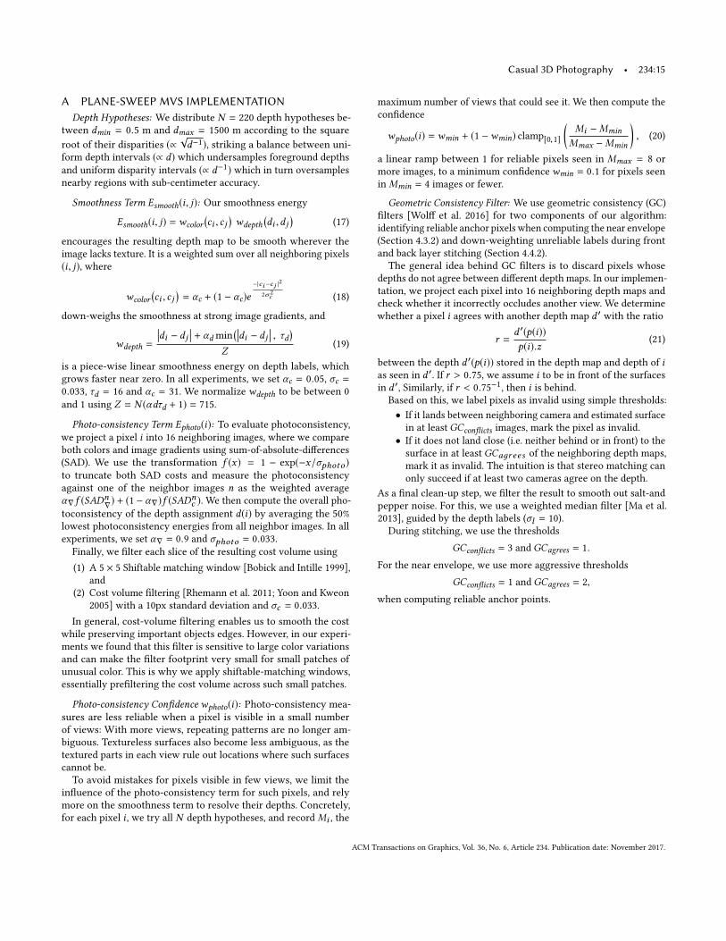
Casual 3D Photography • 234:15
A PLANE-SWEEP MVS IMPLEMENTATIONDepth Hypotheses: We distribute N = 220 depth hypotheses be-
tween dmin = 0.5 m and dmax = 1500 m according to the square
root of their disparities (∝√d−1), striking a balance between uni-
form depth intervals (∝ d) which undersamples foreground depths
and uniform disparity intervals (∝ d−1) which in turn oversamples
nearby regions with sub-centimeter accuracy.
Smoothness Term Esmooth(i, j): Our smoothness energy
Esmooth(i, j) = wcolor(ci , c j
)wdepth
(di ,dj
)(17)
encourages the resulting depth map to be smooth wherever the
image lacks texture. It is a weighted sum over all neighboring pixels
(i, j), where
wcolor(ci , c j
)= αc + (1 − αc)e
−|ci −cj |2
2σ 2
c (18)
down-weighs the smoothness at strong image gradients, and
wdepth =
��di − dj�� + αdmin
(��di − dj�� , τd)
Z(19)
is a piece-wise linear smoothness energy on depth labels, which
grows faster near zero. In all experiments, we set αc = 0.05, σc =0.033, τd = 16 and αc = 31. We normalize wdepth to be between 0
and 1 using Z = N (αdτd + 1) = 715.
Photo-consistency Term Ephoto(i): To evaluate photoconsistency,
we project a pixel i into 16 neighboring images, where we compare
both colors and image gradients using sum-of-absolute-differences
(SAD). We use the transformation f (x) = 1 − exp(−x/σphoto )to truncate both SAD costs and measure the photoconsistency
against one of the neighbor images n as the weighted average
α∇ f (SADn∇) + (1 − α∇)f (SAD
nc ). We then compute the overall pho-
toconsistency of the depth assignment d(i) by averaging the 50%
lowest photoconsistency energies from all neighbor images. In all
experiments, we set α∇ = 0.9 and σphoto = 0.033.Finally, we filter each slice of the resulting cost volume using
(1) A 5 × 5 Shiftable matching window [Bobick and Intille 1999],
and
(2) Cost volume filtering [Rhemann et al. 2011; Yoon and Kweon
2005] with a 10px standard deviation and σc = 0.033.
In general, cost-volume filtering enables us to smooth the cost
while preserving important objects edges. However, in our experi-
ments we found that this filter is sensitive to large color variations
and can make the filter footprint very small for small patches of
unusual color. This is why we apply shiftable-matching windows,
essentially prefiltering the cost volume across such small patches.
Photo-consistency Confidencewphoto(i): Photo-consistency mea-
sures are less reliable when a pixel is visible in a small number
of views: With more views, repeating patterns are no longer am-
biguous. Textureless surfaces also become less ambiguous, as the
textured parts in each view rule out locations where such surfaces
cannot be.
To avoid mistakes for pixels visible in few views, we limit the
influence of the photo-consistency term for such pixels, and rely
more on the smoothness term to resolve their depths. Concretely,
for each pixel i , we try all N depth hypotheses, and recordMi , the
maximum number of views that could see it. We then compute the
confidence
wphoto(i) = wmin + (1 −wmin) clamp[0,1]
(Mi −Mmin
Mmax −Mmin
), (20)
a linear ramp between 1 for reliable pixels seen in Mmax = 8 or
more images, to a minimum confidencewmin = 0.1 for pixels seeninMmin = 4 images or fewer.
Geometric Consistency Filter: We use geometric consistency (GC)
filters [Wolff et al. 2016] for two components of our algorithm:
identifying reliable anchor pixels when computing the near envelope
(Section 4.3.2) and down-weighting unreliable labels during front
and back layer stitching (Section 4.4.2).
The general idea behind GC filters is to discard pixels whose
depths do not agree between different depth maps. In our implemen-
tation, we project each pixel into 16 neighboring depth maps and
check whether it incorrectly occludes another view. We determine
whether a pixel i agrees with another depth map d ′ with the ratio
r =d ′(p(i))
p(i).z(21)
between the depth d ′(p(i)) stored in the depth map and depth of ias seen in d ′. If r > 0.75, we assume i to be in front of the surfaces
in d ′, Similarly, if r < 0.75−1, then i is behind.Based on this, we label pixels as invalid using simple thresholds:
• If it lands between neighboring camera and estimated surface
in at least GCconflicts images, mark the pixel as invalid.
• If it does not land close (i.e. neither behind or in front) to the
surface in at least GCaдr ees of the neighboring depth maps,
mark it as invalid. The intuition is that stereo matching can
only succeed if at least two cameras agree on the depth.
As a final clean-up step, we filter the result to smooth out salt-and
pepper noise. For this, we use a weighted median filter [Ma et al.
2013], guided by the depth labels (σl = 10).
During stitching, we use the thresholds
GCconflicts = 3 and GCagrees = 1.
For the near envelope, we use more aggressive thresholds
GCconflicts = 1 and GCagrees = 2,
when computing reliable anchor points.
ACM Transactions on Graphics, Vol. 36, No. 6, Article 234. Publication date: November 2017.
Top Related