


Languages
Pages
Legal


BUSH 632: Getting Beyond Fear and Loathing of Statistics
Lecture 1
Spring, 2007

Don’t Panic• Motivation: this course is about the
connection between theoretical claims and empirical data
• What we’ll cover (after a very brief review):– Part 1: bi-variate regression– Part 2: multiviariate regression– Part 3: logit analysis and factor analysis
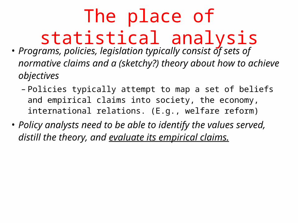
The place of statistical analysis• Programs, policies, legislation typically consist of sets of
normative claims and a (sketchy?) theory about how to achieve objectives– Policies typically attempt to map a set of beliefs and empirical claims
into society, the economy, international relations. (E.g., welfare reform)
• Policy analysts need to be able to identify the values served, distill the theory, and evaluate its empirical claims.

The place of statistical analysis• Ingredients of strong empirical research
–Theory claims for policy (and counter-claims)–Hypotheses measurement analysis–Findings Back to theory…–Implications for policy
•Characterizing data–Data Quality: Valid? Reliable? Relevant?
•Appropriate model design and execution–Are statistical models appropriate to test hypotheses?–Are models appropriately specified?–Do data conform to statistical assumptions?

How to survive this class• Use the webpage
– http://www.tamu.edu/classes/bush/hjsmith/courses/bush632.html
• Lectures and book: as close as possible• Readings: Read ‘em or weep.• Questions: Bring ‘em to class, office hours• Stata: Use it a lot
– In-class examples and exercises
– Download exercises and data in advance
– The place of exercises in Bush 632
• Nothing late; don’t miss class…
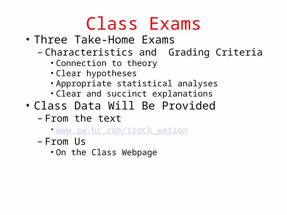
Class Exams• Three Take-Home Exams
– Characteristics and Grading Criteria• Connection to theory• Clear hypotheses• Appropriate statistical analyses• Clear and succinct explanations
• Class Data Will Be Provided– From the text
• www.aw-bc.com/stock_watson– From Us
• On the Class Webpage

A Brief Refresher on Functions and Sampling
• Statistical models involve relationships
– Relationships imply functions
• E.g.: Coffee consumption and productivity
• Functions are ubiquitous (or chaos prevails)
– Most general expression: Y f (X1, X2, … Xn, e)

Linear Functions
Y = 5 + X
0
2
4
6
8
10
12
-6 -4 -2 0 2 4 6
X
Y
X Y-5 0
-4 1
-3 2
-2 3
-1 4
0 5
1 6
2 7
3 8
4 9
5 10

Non-Linear Functions
Y= 3 - Xsqd
-25
-20
-15
-10
-5
0
5
-6 -4 -2 0 2 4 6
Y
X Y-5 -22
-4 -13
-3 -6
-2 -1
-1 2
0 3
1 2
2 -1
3 -6
4 -13
5 -22
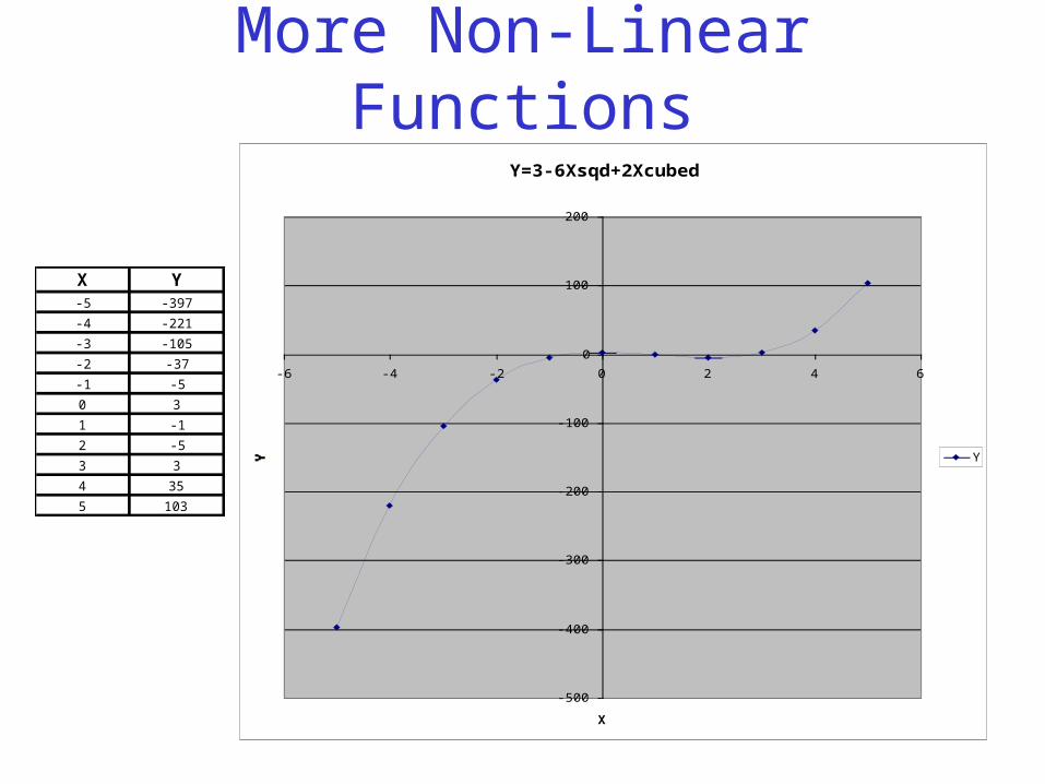
More Non-Linear FunctionsY=3-6Xsqd+2Xcubed
-500
-400
-300
-200
-100
0
100
200
-6 -4 -2 0 2 4 6
X
Y Y
X Y-5 -397
-4 -221
-3 -105
-2 -37
-1 -5
0 3
1 -1
2 -5
3 3
4 35
5 103

Functions in Policy
• Welfare and work incentives– Employment = f(welfare programs, …) Pretty complex
• Nuclear deterrence– Major power military conflict = f(nuclear capabilities, proliferation, …)
• Educational Attainment– Test Scores = f(class size, institutional incentives, …)
• Successful Program Implementation– Implementation = f(clarity, public support, complexity…)

Sampling is also ubiquitous• “Knowing” a person: we sample
• “Knowing” places: we sample
• Samples are necessary to identify functions– Samples must cover relevant variables,
contexts, etc.
• Strategies for sampling– Soup and temperature: stir it– Stratify sample: observations in appropriate
“cells”– Randomize

Statistics Refresher: Topics• Central tendency
– Expected value and means
• Dispersion– Population variance,
sample variance, standard deviations
• Measures of relations• Covariation
– covariance matrices
• Correlations• Sampling
distributions
• Characteristics of sampling distributions
• Class Data– 2005 National Security Survey
(phone and web)
– Stata application
• Means, Variance, Standard Deviations
• The Normal Distribution
• Medians and IQRs
• Box Plots and Symmetry Plots
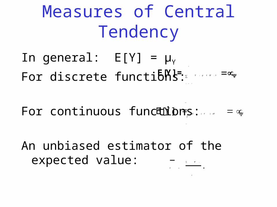
Measures of Central Tendency
In general: E[Y] = µY
For discrete functions:
For continuous functions:
An unbiased estimator of the expected value:
E[Y] = Y i
i = 1
I
∑ f ( Y i ) = µY
E[Y] = Yf ( Y ) dY
−∞
+∞
∫ = µY
Y =
∑ Y i
n
.
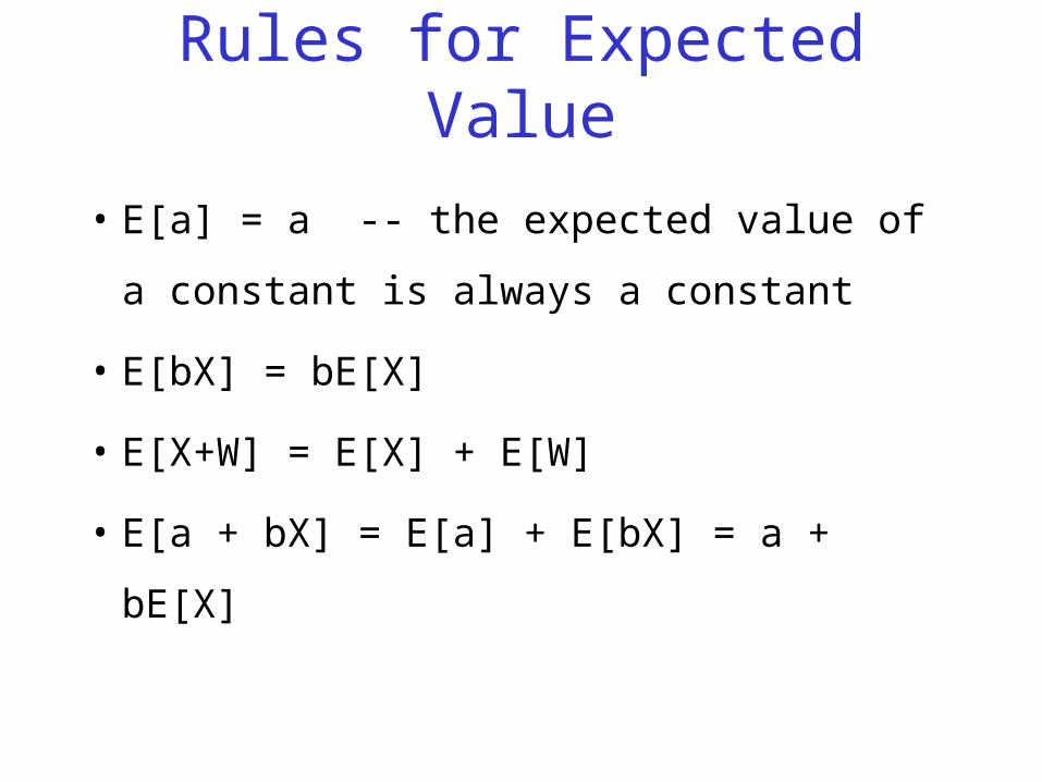
Rules for Expected Value
• E[a] = a -- the expected value of a constant
is always a constant
• E[bX] = bE[X]
• E[X+W] = E[X] + E[W]
• E[a + bX] = E[a] + E[bX] = a + bE[X]
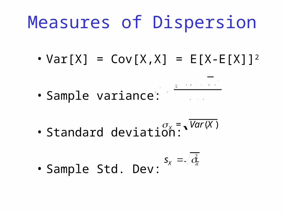
Measures of Dispersion
• Var[X] = Cov[X,X] = E[X-E[X]]2
• Sample variance:
• Standard deviation:
• Sample Std. Dev:
sX
2
=
( Xi
− X )
2
∑
n − 1
σ X = Var (X )
sX = sX2

Rules for Variance Manipulation
• Var[a] = 0
• Var[bX] = b2 Var[X]
• From which we can deduce:
Var[a+bX] = Var[a] + Var[bX] = b2 Var[X]
• Var[X + W]
= Var[X] + Var[W] + 2Cov[X,W]
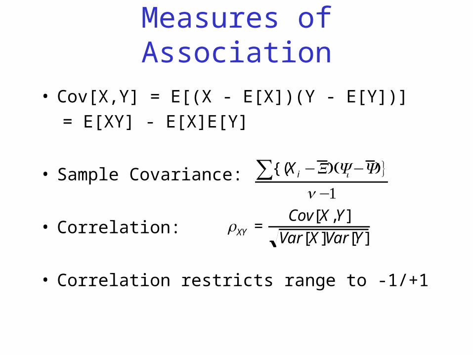
Measures of Association
• Cov[X,Y] = E[(X - E[X])(Y - E[Y])]
= E[XY] - E[X]E[Y]
• Sample Covariance:
• Correlation:
• Correlation restricts range to -1/+1
{(X i −X)(Yi −Y)}∑n−1
ρXY =Cov[X,Y]
Var [X]Var [Y]

Rules of Covariance Manipulation
• Cov[a,Y] = 0 (why?)
• Cov[bX,Y] = bCov[X,Y] (why?)
• Cov[X + W,Y] = Cov[X,Y] + Cov[W,Y]
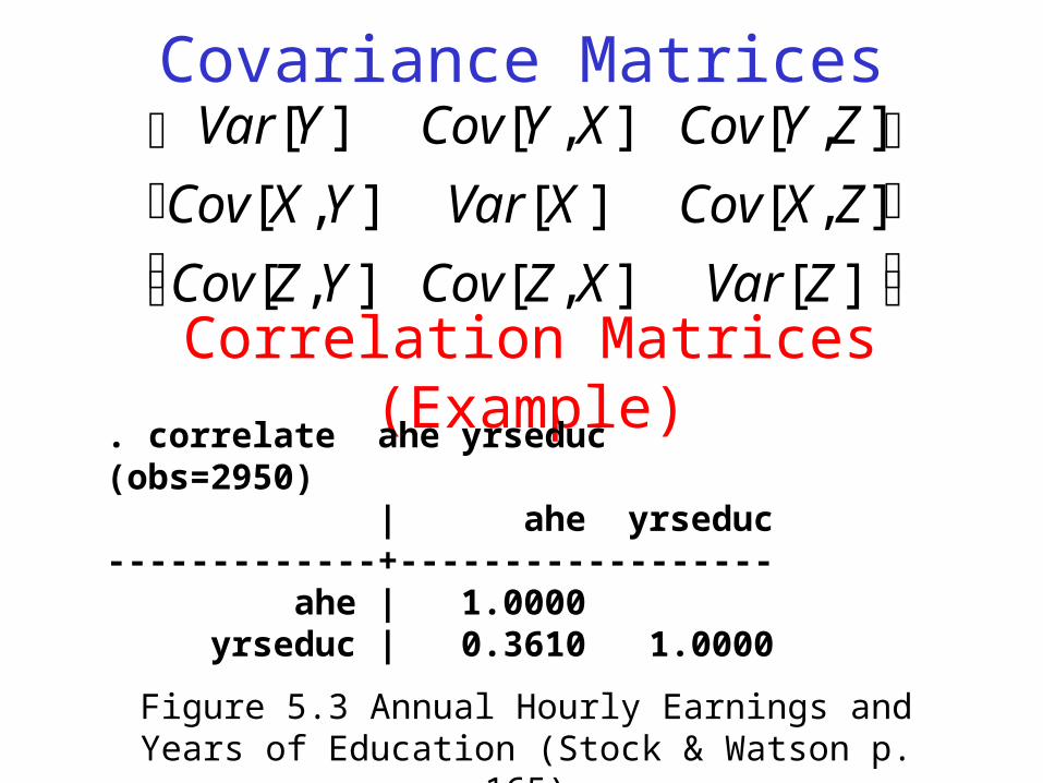
Var [Y ] Cov[Y , X] Cov[Y ,Z ]
Cov[X,Y ] Var [X ] Cov[X, Z]
Cov[Z,Y ] Cov[Z, X] Var [Z ]
⎡
⎣
⎢ ⎢
⎤
⎦
⎥ ⎥
Covariance Matrices
Correlation Matrices (Example). correlate ahe yrseduc(obs=2950) | ahe yrseduc-------------+------------------ ahe | 1.0000 yrseduc | 0.3610 1.0000
Figure 5.3 Annual Hourly Earnings and Years of Education (Stock & Watson p. 165)
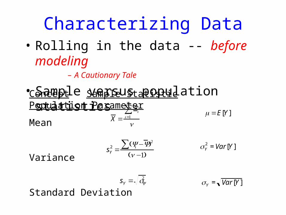
Characterizing Data• Rolling in the data -- before modeling
– A Cautionary Tale
• Sample versus population statisticsConcept Sample Statistic Population Parameter
Mean
Variance
Standard Deviation
X =Xi
i=1
n
∑n
μ =E[Y ]
sY2 =
(Yi∑ −Y)2
(n−1)σY
2 = Var [Y ]
sY = sY2
σY = Var [Y ]

Properties of Standard Normal (Gaussian) Distributions
• Can be dramatically different than sample frequencies (especially small ones) Stata
• Tails go to plus/minus infinity
• The density of the distribution is key:+/- 1.96 std.s covers 95% of the distribution
+/- 2.58 std.s covers 99% of the distribution
• Student’s t tables converge on Gaussian
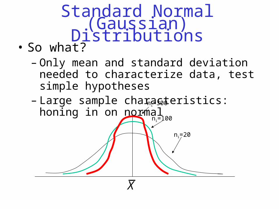
Standard Normal (Gaussian) Distributions
• So what?– Only mean and standard deviation needed to
characterize data, test simple hypotheses– Large sample characteristics: honing in on normal
ni=300
ni=100
ni=20
X
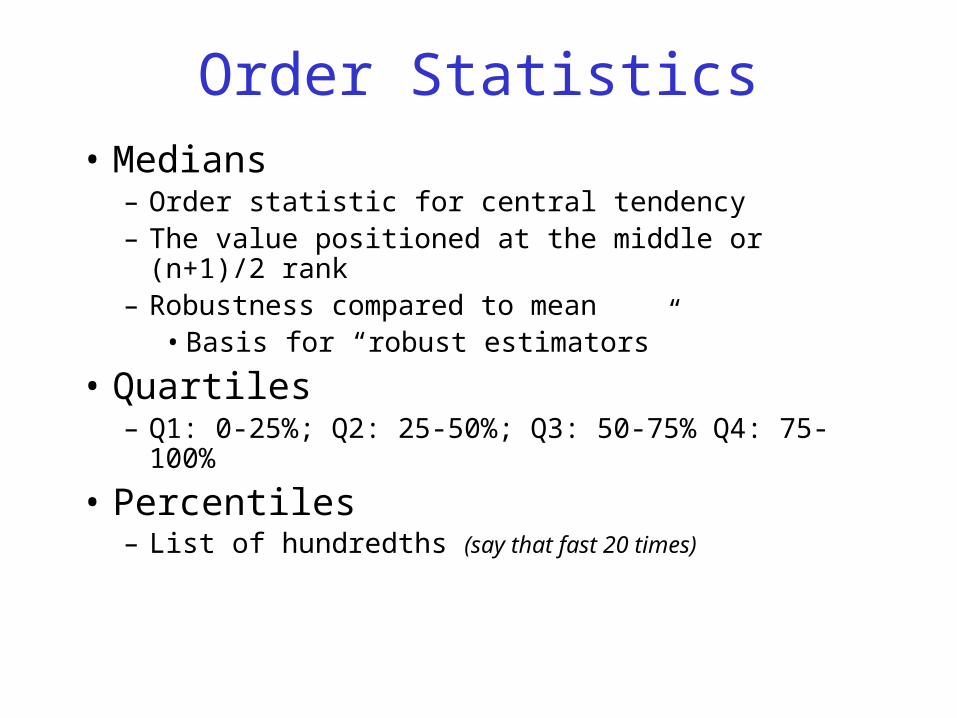
Order Statistics• Medians
– Order statistic for central tendency– The value positioned at the middle or (n+1)/2 rank– Robustness compared to mean
• Basis for “robust estimators”
• Quartiles– Q1: 0-25%; Q2: 25-50%; Q3: 50-75% Q4: 75-100%
• Percentiles– List of hundredths (say that fast 20 times)
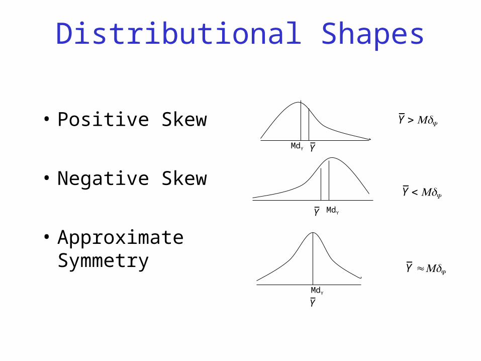
Distributional Shapes
• Positive Skew
• Negative Skew
• Approximate Symmetry
MdY
MdY
MdY
Y
Y
Y
Y >MdY
Y <MdY
Y ≈MdY
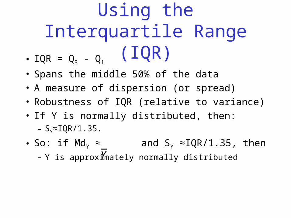
Using the Interquartile Range (IQR)
• IQR = Q3 - Q1
• Spans the middle 50% of the data• A measure of dispersion (or spread)• Robustness of IQR (relative to variance)• If Y is normally distributed, then:
– SY≈IQR/1.35.
• So: if MdY ≈ and SY ≈IQR/1.35, then– Y is approximately normally distributed
Y
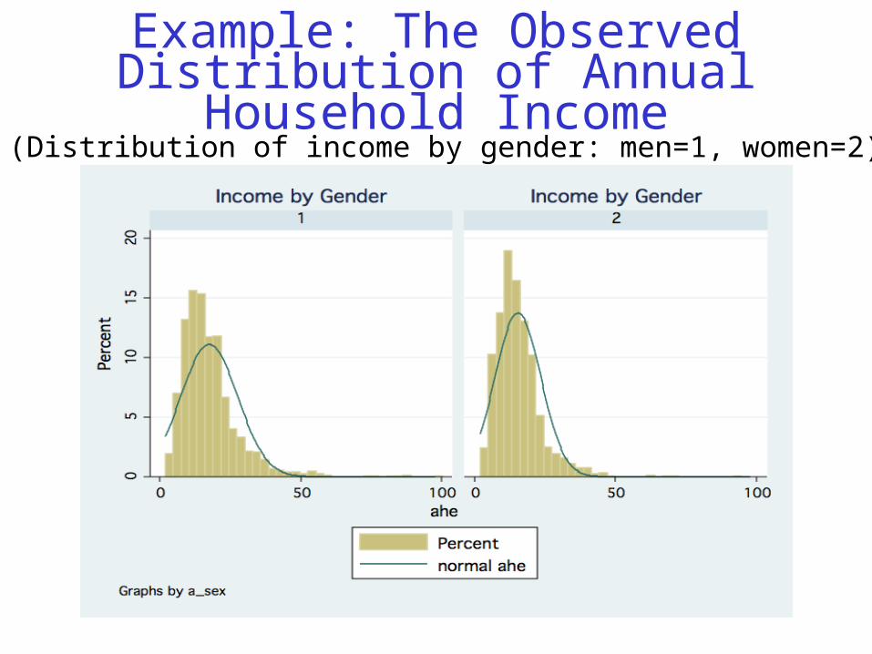
Example: The Observed Distribution of Annual Household Income
(Distribution of income by gender: men=1, women=2)
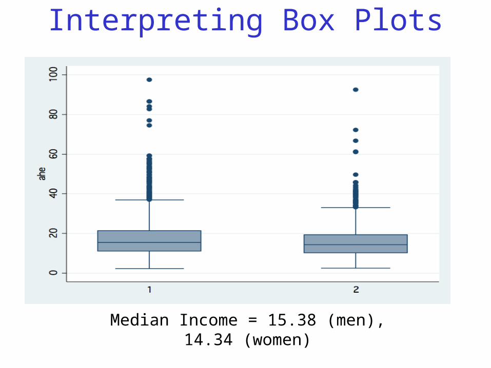
Interpreting Box Plots
Median Income = 15.38 (men), 14.34 (women)
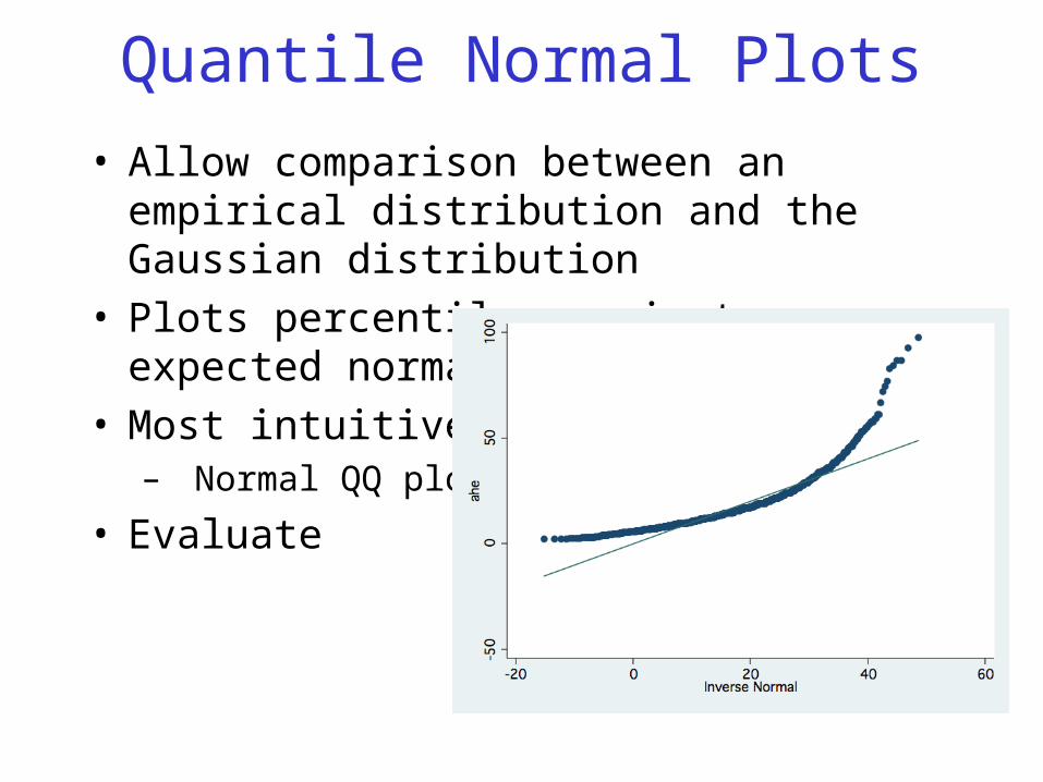
Quantile Normal Plots
• Allow comparison between an empirical distribution and the Gaussian distribution
• Plots percentiles against expected normal• Most intuitive:
– Normal QQ plots
• Evaluate

Data Exploration in Stata• Access The Guns dataset from the replication data on the
Stock and Watson Webpage
• Using Incarceration Rate: univariate analysis Stata
• Using Incarceration Rate : split by Shall Issue Laws
Stata
• Exercises:
– Graphing: Produce
• Histograms
• Box plots
• Q-Normal plots

For Next Week• Read Stock and Watson
– Chapter 4
• Homework Assignment on Webpage
Top Related