


Languages
Pages
Legal


BUFFETING RESPONSE PREDICTION BUFFETING RESPONSE PREDICTION FOR CABLEFOR CABLE--STAYED BRIDGESSTAYED BRIDGES
LE THAI HOALE THAI HOAKyoto UniversityKyoto University
CONTENTSCONTENTS
1. Introduction1. Introduction2. Literature review on buffeting response 2. Literature review on buffeting response
analysis for bridgesanalysis for bridges3. Basic formations of buffeting response3. Basic formations of buffeting response4. Analytical method for buffeting response 4. Analytical method for buffeting response
prediction in frequency domainprediction in frequency domain5. Numerical example and discussions5. Numerical example and discussions6. Conclusion6. Conclusion
1
INTRODUCTIONINTRODUCTION
2
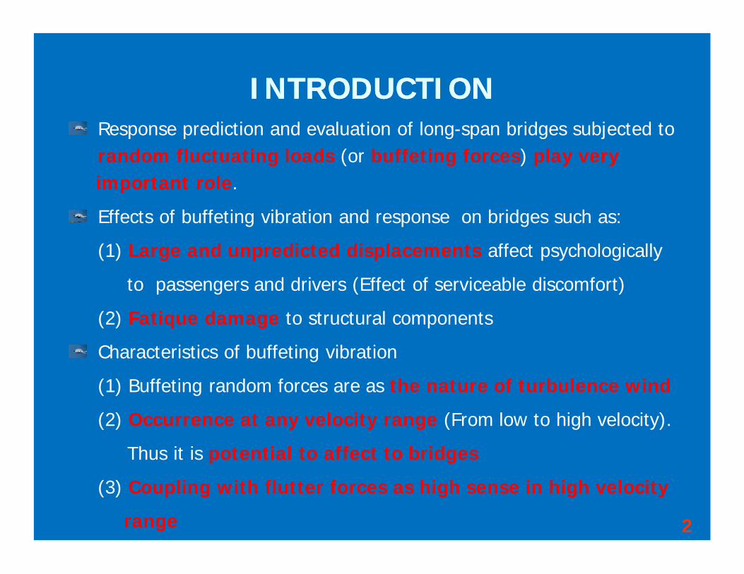
Response prediction and evaluation of long-span bridges subjected torandom fluctuating loads (or buffeting forces) play very important role.
Effects of buffeting vibration and response on bridges such as:
(1) Large and unpredicted displacements affect psychologically
to passengers and drivers (Effect of serviceable discomfort)
(2) Fatique damage to structural components
Characteristics of buffeting vibration
(1) Buffeting random forces are as the nature of turbulence wind
(2) Occurrence at any velocity range (From low to high velocity).
Thus it is potential to affect to bridges
(3) Coupling with flutter forces as high sense in high velocity
range
WINDWIND--INDUCED VIBRATIONS INDUCED VIBRATIONS
3
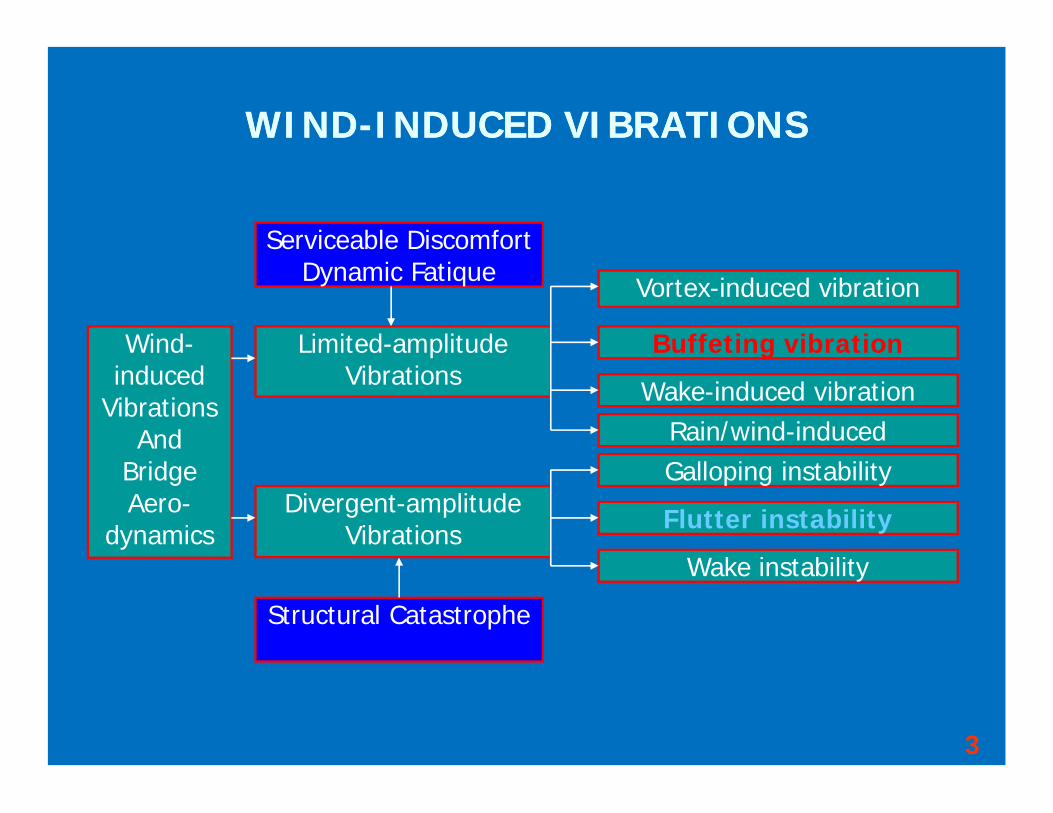
Wind-induced
VibrationsAnd
Bridge Aero-
dynamics
Limited-amplitude Vibrations
Divergent-amplitude Vibrations
Vortex-induced vibration
Buffeting vibration
Wake-induced vibrationRain/wind-inducedGalloping instability
Flutter instability
Wake instability
Serviceable DiscomfortDynamic Fatique
Structural Catastrophe

Limited-amplitude Response Divergent-amplitude Response
ResponseAmplitude
Flutter and GallopingInstabilities
Buffeting Response
‘Lock-in’ Response
Karman-inducedResponse
ResonancePeak Value
4
RESPONSE AMPLITUDE AND VELOCITYRESPONSE AMPLITUDE AND VELOCITY
Reduced Velocity
Random Forcesin Turbulence Wind
Vortex-induced Response
Forced Forces
Self-excited Forcesin Smooth or
Turbulence Wind
nBUU re
Self-excitedForces
Low and medium velocity range High velocity range
Note: Classification of low, medium and high velocity ranges is relative together
INTERACTION OF WINDINTERACTION OF WIND--INDUCED VIBRATIONSINDUCED VIBRATIONS
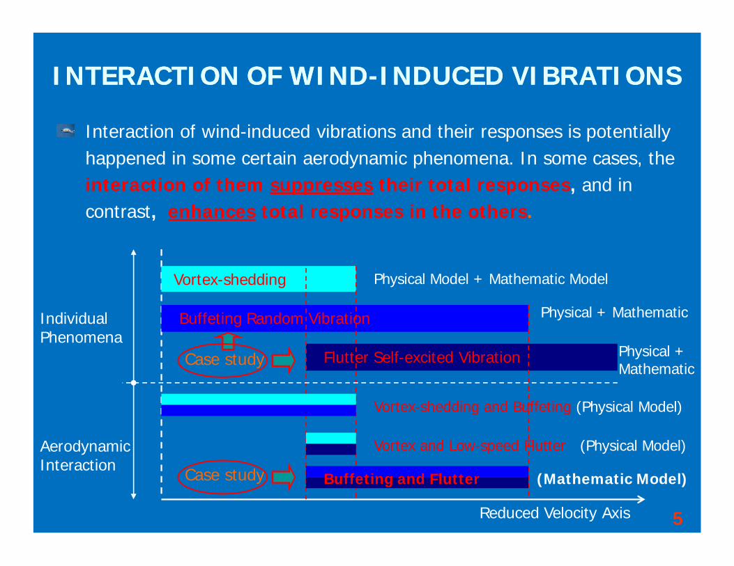
Interaction of wind-induced vibrations and their responses is potentially happened in some certain aerodynamic phenomena. In some cases, theinteraction of them suppresses their total responses, and incontrast, enhances total responses in the others.
5Reduced Velocity Axis
Vortex-shedding
Buffeting Random Vibration
Flutter Self-excited Vibration
AerodynamicInteraction
IndividualPhenomena
Vortex-shedding and Buffeting (Physical Model)
Vortex and Low-speed Flutter (Physical Model)
Buffeting and Flutter (Mathematic Model)
Physical Model + Mathematic Model
Physical + Mathematic
Physical +Mathematic
Case study
Case study
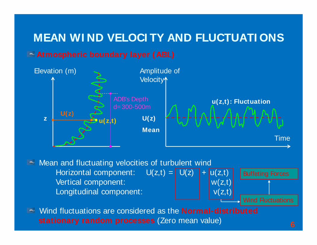
MEAN WIND VELOCITY AND FLUCTUATIONSMEAN WIND VELOCITY AND FLUCTUATIONS
Mean and fluctuating velocities of turbulent wind Horizontal component: U(z,t) = U(z) + u(z,t) Vertical component: w(z,t)Longitudinal component: v(z,t)
Wind fluctuations are considered as the Normal-distributed stationary random processes (Zero mean value)
Atmospheric boundary layer (ABL)
6
Elevation (m)
ADB’s Depth d=300-500m
U(z)u(z,t)
Amplitude of Velocity
Time
U(z)
Mean
u(z,t): Fluctuation
z
Wind Fluctuations
Buffeting Forces

WIND FORCES AND RESPONSEWIND FORCES AND RESPONSE
)()()( nFtFFtF SEBQStotal
Total wind forces acting on structures can be computed under
superposition principle of aerodynamic forces as follows
QSF : Quasi-steady aerodynamic forces (Static wind forces)
)(nFSE : Self-controlled aerodynamic forces (Flutter)
)(tFB : Unsteady (random) aerodynamic forces (Buffeting)
Aerodynamic behaviors of structures can be estimated under static
equilibrium equations and aerodynamic motion equations
QSFKX
)()( tFnFKXXCXM BSE
: Static Equilibrium
: Dynamic Equilibrium
Combination of self-controlled forces (Flutter) and unsteady fluctuating
forces (Buffeting) is favorable under high-velocity range7
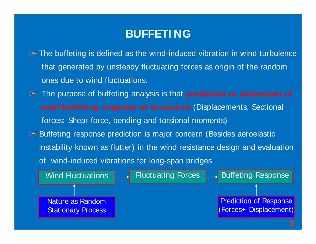
BUFFETING BUFFETING
The buffeting is defined as the wind-induced vibration in wind turbulence
that generated by unsteady fluctuating forces as origin of the random
ones due to wind fluctuations.
The purpose of buffeting analysis is that prediction or estimation of
total buffeting response of structures (Displacements, Sectional
forces: Shear force, bending and torsional moments)
Buffeting response prediction is major concern (Besides aeroelastic
instability known as flutter) in the wind resistance design and evaluation
of wind-induced vibrations for long-span bridges
8
Wind Fluctuations Fluctuating Forces Buffeting Response
Nature as Random Stationary Process
Prediction of Response (Forces+ Displacement)
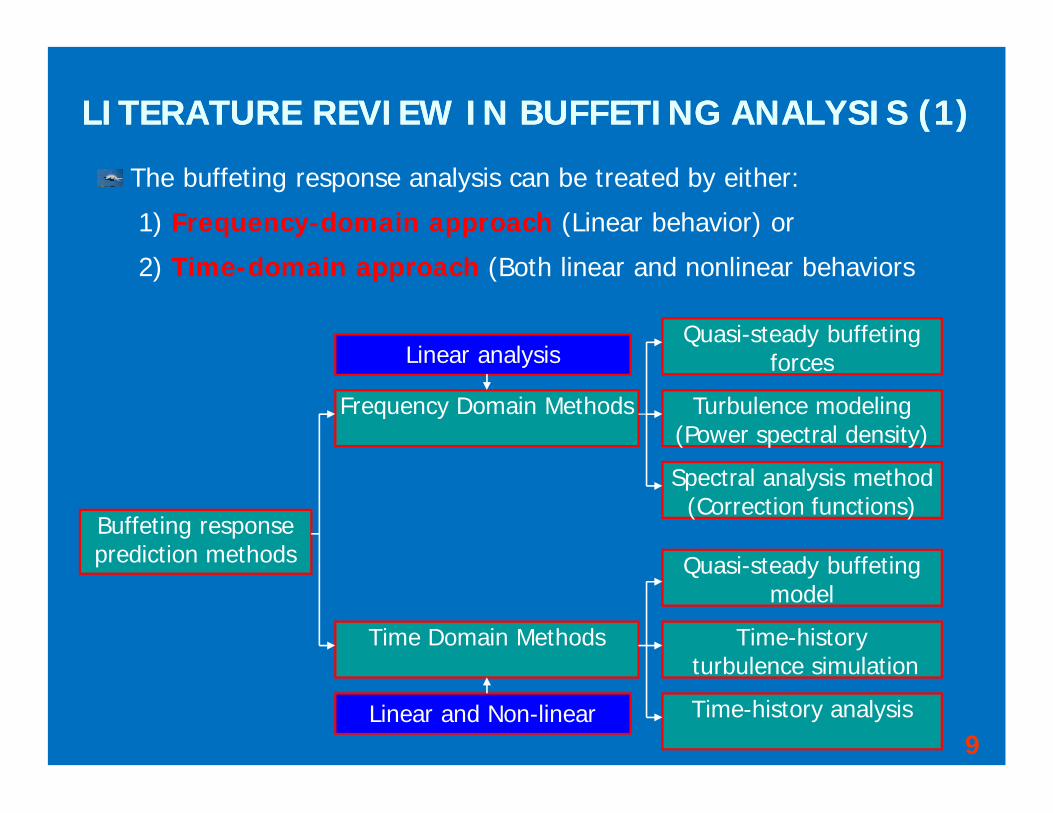
LITERATURE REVIEW IN BUFFETING ANALYSIS (1) LITERATURE REVIEW IN BUFFETING ANALYSIS (1)
The buffeting response analysis can be treated by either:
1) Frequency-domain approach (Linear behavior) or
2) Time-domain approach (Both linear and nonlinear behaviors
Buffeting response prediction methods
Frequency Domain Methods
Time Domain Methods
Quasi-steady buffeting forces
Turbulence modeling(Power spectral density)
Spectral analysis method(Correction functions)
Quasi-steady buffeting model
Time-historyturbulence simulation
Time-history analysis 9
Linear analysis
Linear and Non-linear
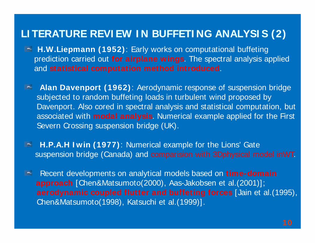
LITERATURE REVIEW IN BUFFETING ANALYSIS (2)LITERATURE REVIEW IN BUFFETING ANALYSIS (2)H.W.Liepmann (1952): Early works on computational buffeting
prediction carried out for airplane wings. The spectral analysis appliedand statistical computation method introduced.
Alan Davenport (1962): Aerodynamic response of suspension bridgesubjected to random buffeting loads in turbulent wind proposed by Davenport. Also cored in spectral analysis and statistical computation, butassociated with modal analysis. Numerical example applied for the FirstSevern Crossing suspension bridge (UK).
H.P.A.H Iwin (1977): Numerical example for the Lions’ Gate suspension bridge (Canada) and comparision with 3Dphysical model inWT.
Recent developments on analytical models based on time-domain approach [Chen&Matsumoto(2000), Aas-Jakobsen et al.(2001)];aerodynamic coupled flutter and buffeting forces [Jain et al.(1995),Chen&Matsumoto(1998), Katsuchi et al.(1999)].
10

EXISTING ASSUMPTIONS IN BUFFETING ANALYSIS EXISTING ASSUMPTIONS IN BUFFETING ANALYSIS
(1) Gaussian stationary processes of wind fluctuationsWind fluctuations treated as Gaussian stationary random processes
(2) Quasi-steady assumption Unsteady buffeting loads modeled as quasi-steady forces by some simple approximations: i) Relative velocity and ii) Unsteady force coefficients
(3) Strip assumption Unsteady buffeting forces on any strip are produced by only the windfluctuation acting on this strip that can be representative for whole structure
(4) Correction functions and transfer functionSome correction functions (Aerodynamic Admittance, Coherence, Joint Acceptance Function) and transfer function (Mechanical Admittance) added for transform of statistical computation and SISO
(5) Modal uncoupling: Multimodal superposition from generalized response
is validated 10
TIMETIME--FREQUENCY DOMAIN TRANFORMATION FREQUENCY DOMAIN TRANFORMATION AND POWER SPECTRUMAND POWER SPECTRUM
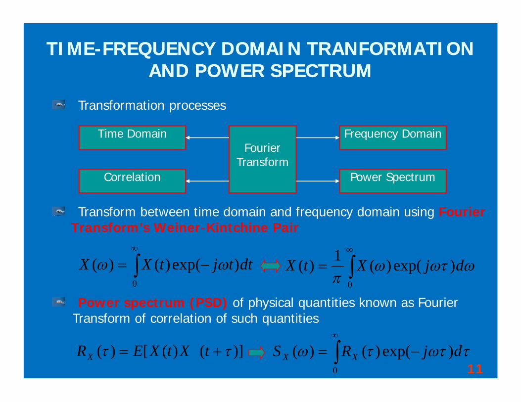
Transformation processes
Time Domain Frequency Domain
Correlation Power Spectrum
Fourier Transform
Transform between time domain and frequency domain using Fourier Transform’s Weiner-Kintchine Pair
0
)exp()()( dttjtXX
0
)exp()(1)(
djXtX
Power spectrum (PSD) of physical quantities known as FourierTransform of correlation of such quantities
0
)exp()()( djRS XX)]()([)( tXtXERX11
BASIC FORMATIONS OF BUFFETING BASIC FORMATIONS OF BUFFETING RESPONSE ANALYSIS RESPONSE ANALYSIS
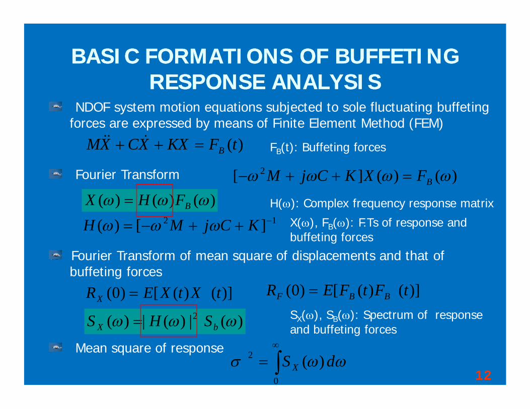
NDOF system motion equations subjected to sole fluctuating buffeting forces are expressed by means of Finite Element Method (FEM)
)(tFKXXCXM B
Fourier Transform )()(][ 2 BFXKCjM )()()( BFHX
12 ][)( KCjMH H(): Complex frequency response matrix
Fourier Transform of mean square of displacements and that of buffeting forces
FB(t): Buffeting forces
)]()([)0( tXtXERX
)(|)(|)( 2 bX SHS
X(), FB(): F.Ts of response and buffeting forces
)]()([)0( tFtFER BBF SX(), SB(): Spectrum of response and buffeting forces
Mean square of response
0
2 )( dS X12
MULTIMODE ANALYTICAL METHOD OF MULTIMODE ANALYTICAL METHOD OF BRIDGES IN FREQUENCY DOMAINBRIDGES IN FREQUENCY DOMAIN
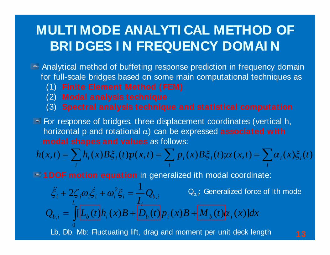
Analytical method of buffeting response prediction in frequency domain for full-scale bridges based on some main computational techniques as
(1) Finite Element Method (FEM)(2) Modal analysis technique(3) Spectral analysis technique and statistical computation
For response of bridges, three displacement coordinates (vertical h, horizontal p and rotational ) can be expressed associated with modal shapes and values as follows:
;)()(),( i
ii tBxhtxh ;)()(),( i
ii tBxptxp i
ii txtx )()(),(
1DOF motion equation in generalized ith modal coordinate:
ibi
iiiiii QI ,
2 12
L
ibibibib dxxtMBxptDBxhtLQ0
, )]()()()()()([
Qb,i: Generalized force of ith mode
Lb, Db, Mb: Fluctuating lift, drag and moment per unit deck length 13

RELATION SPECTRA OF RESPONSE AND FORCESRELATION SPECTRA OF RESPONSE AND FORCESAND BUFFETING FORCE MODELAND BUFFETING FORCE MODEL
])()(2[21)( '
02
UtwC
UtuCBUtL LLb
])()(2[21)( '
02
UtwC
UtuCBUtD DDb
Transform 1DOF motion equation in generalized ith modal coordinateinto spectrum form :
)(|)(|)( ,2
, nSnHnS kbkk 1
2
222
2
222 ]}4)1[({|)(|
kk
kkk n
nnnInH
k=h; p;
Fluctuating buffeting forces (Lift, Drag and Moment) per unit deck length can be determined as follows due to the Quasi-steady Assumption
])()(2[21)( '
022
UtwC
UtuCBUtM MMb
u(t), w(t): Horizontal and vertical fluctuations
Spectrum of Forces
14
Mechanical Admittance
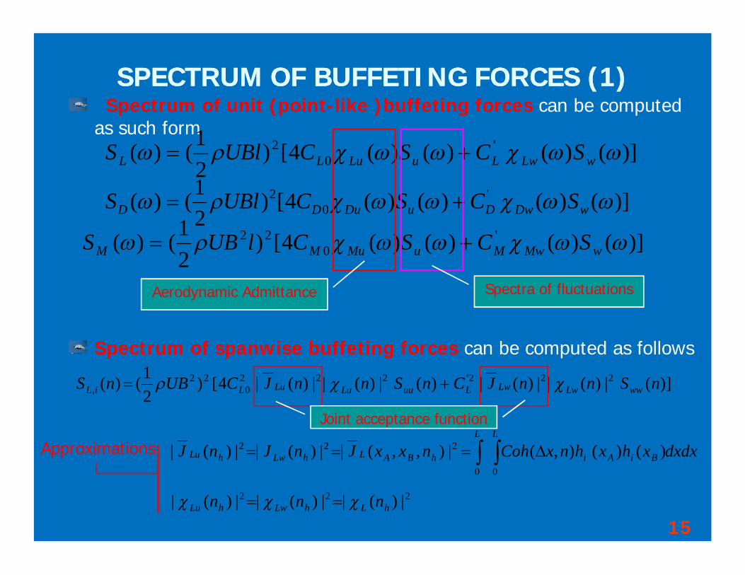
SPECTRUM OF BUFFETING FORCES (1)SPECTRUM OF BUFFETING FORCES (1)Spectrum of unit (point-like )buffeting forces can be computed
as such form)]()()()(4[)
21()( '
02 wLwLuLuLL SCSCUBlS
)]()()()(4[)21()( '
02 wDwDuDuDD SCSCUBlS
)]()()()(4[)21()( '
022 wMwMuMuMM SCSClUBS
Spectra of fluctuationsAerodynamic Admittance
Spectrum of spanwise buffeting forces can be computed as follows
)](|)(||)(|)(|)(||)(|4[)21()( 222'222
022
, nSnnJCnSnnJCUBnS wwLwLwLuuLuLuLiL
dxdxxhxhnxCohnxxJnJnJL
BiAi
L
hBALhLwhLu 00
222 )()(),(|),,(||)(||)(|
222 |)(||)(||)(| hLhLwhLu nnn
Joint acceptance function
Approximations
15

SPECTRUM OF BUFFETING FORCES (2)SPECTRUM OF BUFFETING FORCES (2)Spectrum of spanwise buffeting forces can be expressed
222
22
2
21
, |)(||)(|)]()(4[)( hLhLhwhuiL nnJnSULnS
ULnS
222
22
2
21
, |)(||)(|)]()(4[)( pDpDpwpuiD nnJnSUDnS
UDnS
222
22
2
21
, |)(||)(|)]()(4
[)( nnJnSUMnS
UMnS MMwuiM
20
21 2
1 BCUL L2'2
2 21 BCUL L
20
21 2
1 BCUD D 2'22 2
1 BCUD D
20
21 2
1 BCUM M2'2
2 21 BCUM D
16
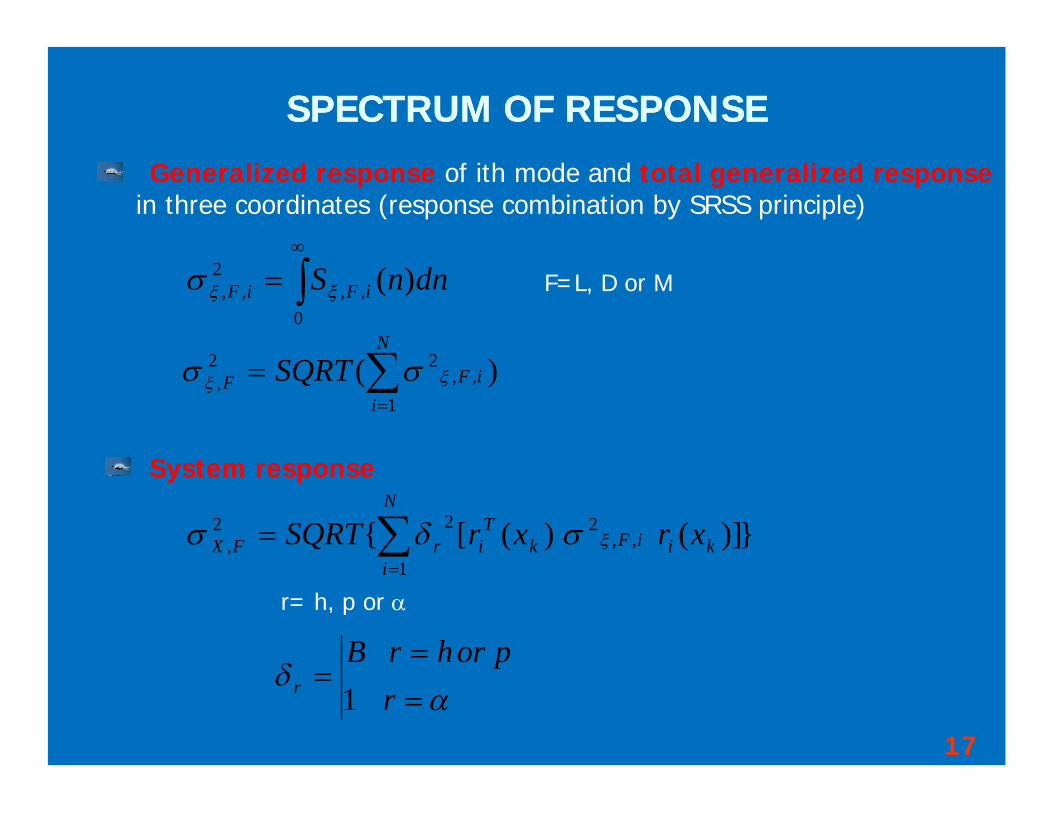
SPECTRUM OF RESPONSE SPECTRUM OF RESPONSE
Generalized response of ith mode and total generalized responsein three coordinates (response combination by SRSS principle)
0
,,2
,, )( dnnS iFiF F=L, D or M
System response
)(1
,,22
,
N
iiFF SQRT
})]()([{1
,,222
,
N
ikiiFk
TirFX xrxrSQRT
r
porhrBr 1
r= h, p or
17
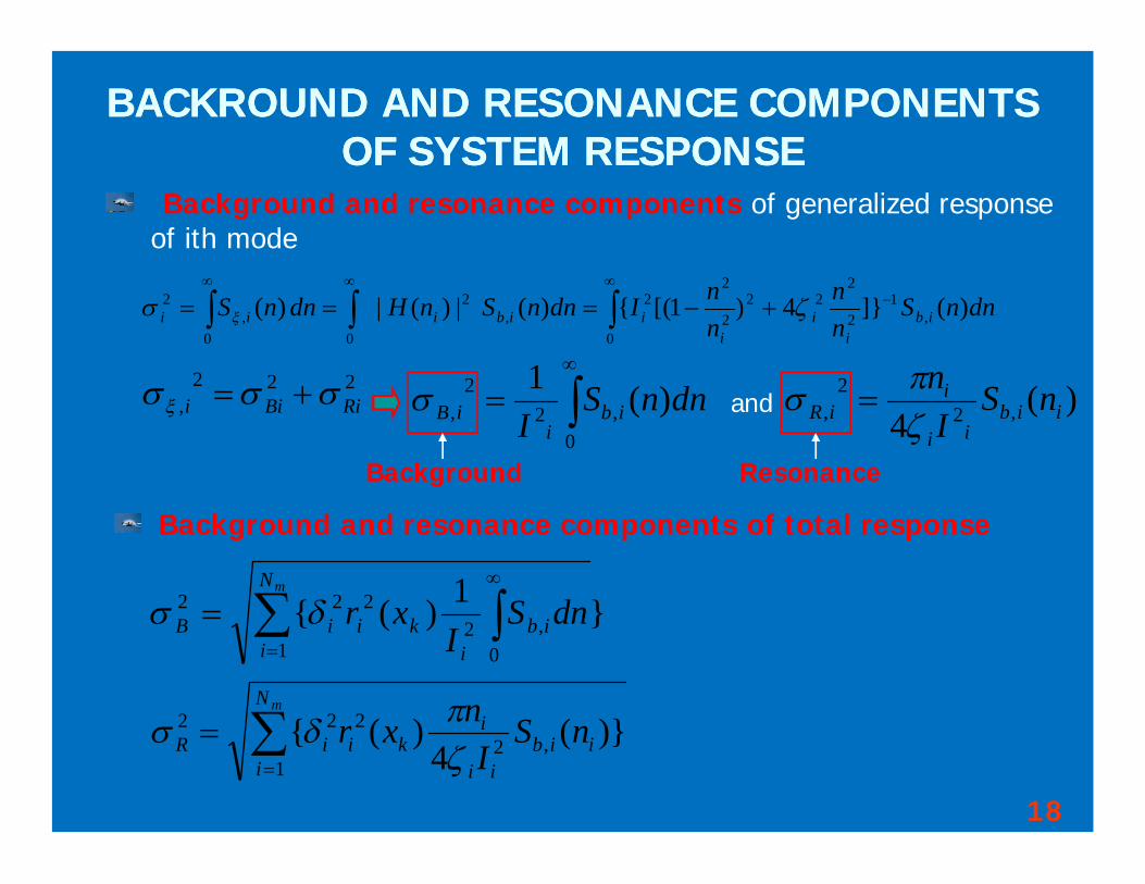
BACKROUND AND RESONANCE COMPONENTS BACKROUND AND RESONANCE COMPONENTS OF SYSTEM RESPONSEOF SYSTEM RESPONSE
Background and resonance components of generalized responseof ith mode
0
,1
2
222
2
22
,2
00,
2 )(]}4)1[({)(|)(|)( dnnSnn
nnIdnnSnHdnnS ib
ii
iiibiii
222, RiBii
0
,22
, )(1 dnnSI ib
iiB )(
4 ,22
, iibii
iiR nS
In
and
Background and resonance components of total response
}1)({1 0
,2222
mN
iib
ikiiB dnS
Ixr
Background Resonance
mN
iiib
ii
ikiiR nS
Inxr
1,2
222 )}(4
)({
18
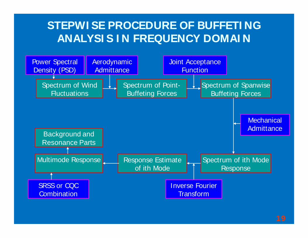
Spectrum of Wind Fluctuations
Spectrum of Point-Buffeting Forces
Spectrum of Spanwise Buffeting Forces
Spectrum of ith Mode Response
Response Estimateof ith Mode
Aerodynamic Admittance
Joint Acceptance Function
Mechanical Admittance
Power Spectral Density (PSD)
Multimode Response
Inverse Fourier Transform
STEPWISE PROCEDURE OF BUFFETING STEPWISE PROCEDURE OF BUFFETING ANALYSIS IN FREQUENCY DOMAINANALYSIS IN FREQUENCY DOMAIN
SRSS or CQCCombination
Background and Resonance Parts
19
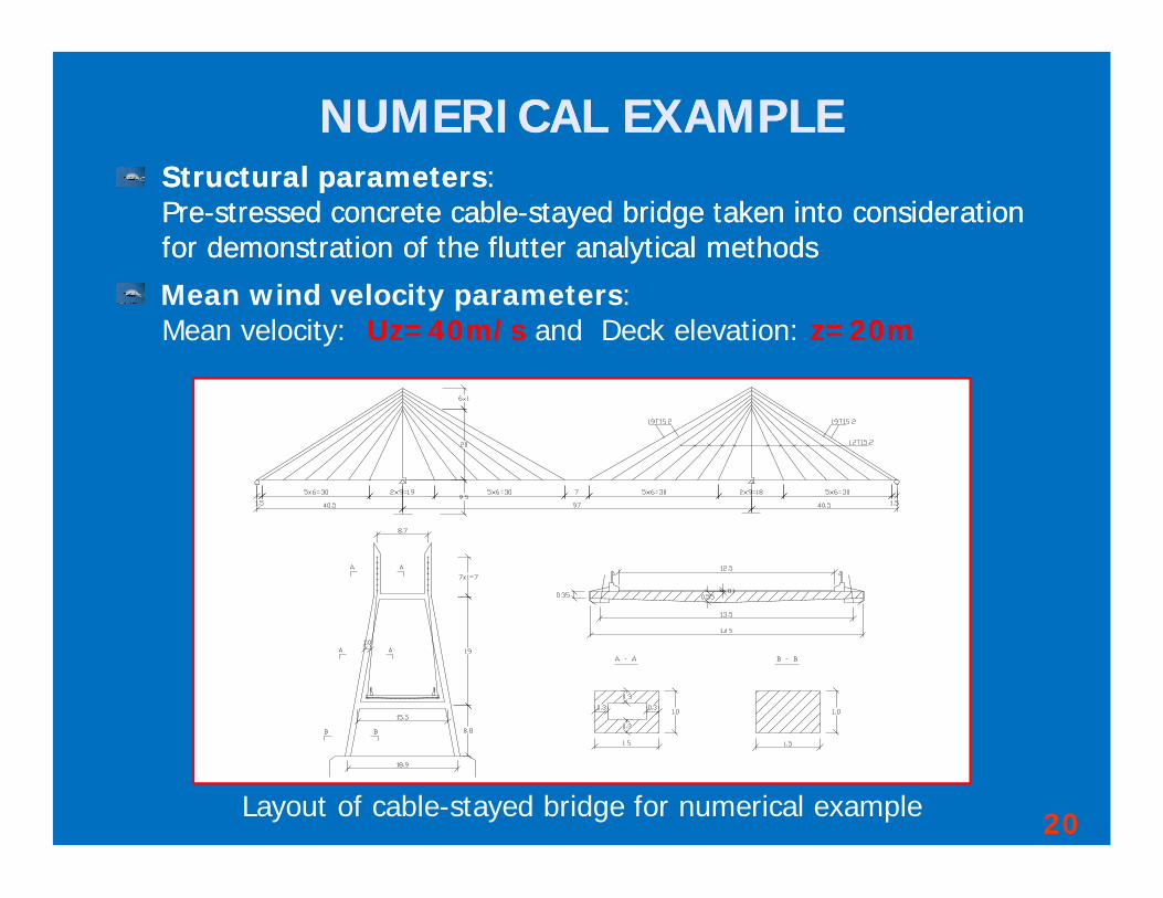
Structural parametersStructural parameters: : PPrere--stressed concrete cablestressed concrete cable--stayed bridge taken into considerationstayed bridge taken into considerationfor demonstration of the flutter analytical methodsfor demonstration of the flutter analytical methods
Layout of cable-stayed bridge for numerical example
NUMERICAL EXAMPLE NUMERICAL EXAMPLE
Mean wind velocity parameters:Mean velocity: Uz=40m/s and Deck elevation: z=20m
20
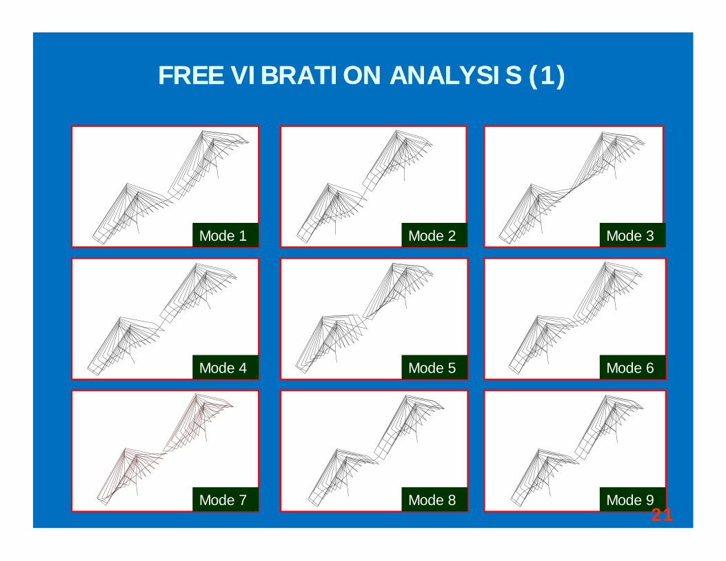
FREE VIBRATION ANALYSIS (1)FREE VIBRATION ANALYSIS (1)
Mode 1 Mode 2 Mode 3
Mode 4 Mode 5 Mode 6
Mode 7 Mode 8 Mode 921
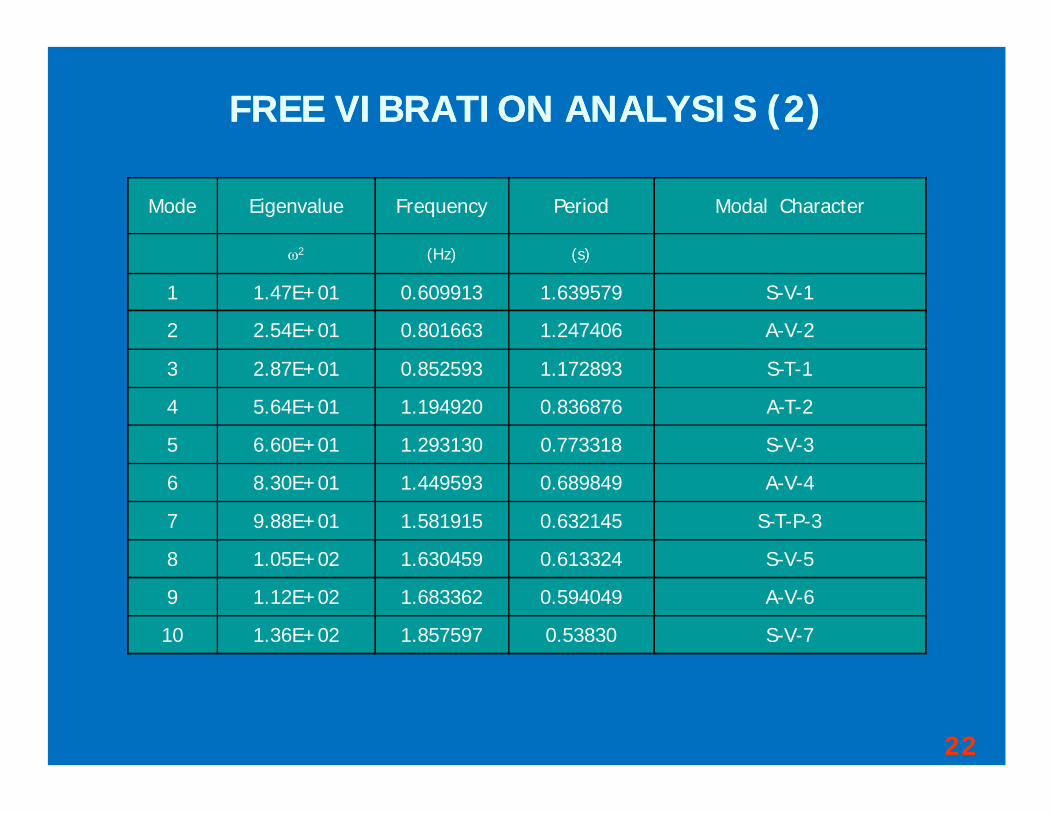
Mode Eigenvalue Frequency Period Modal Character
2 (Hz) (s)
1 1.47E+01 0.609913 1.639579 S-V-1
2 2.54E+01 0.801663 1.247406 A-V-2
3 2.87E+01 0.852593 1.172893 S-T-1
4 5.64E+01 1.194920 0.836876 A-T-2
5 6.60E+01 1.293130 0.773318 S-V-3
6 8.30E+01 1.449593 0.689849 A-V-4
7 9.88E+01 1.581915 0.632145 S-T-P-3
8 1.05E+02 1.630459 0.613324 S-V-5
9 1.12E+02 1.683362 0.594049 A-V-6
10 1.36E+02 1.857597 0.53830 S-V-7
FREE VIBRATION ANALYSIS (2)FREE VIBRATION ANALYSIS (2)
22

MODAL SUM COEFFICIENTS MODAL SUM COEFFICIENTS
Mode Frequency Modal Modal integral sums Grmsn
shape (Hz) Character Ghihi Gpipi Gii
1 0.609913 S-V-1 5.20E-01 7.50E-11 0.00E+00
2 0.801663 A-V-2 4.95E-01 7.43E-09 1.35E-09
3 0.852593 S-T-1 3.79E-09 5.23E-05 1.14E-02
4 1.194920 A-T-2 1.78E-07 1.82E-05 1.07E-02
5 1.293130 S-V-3 5.07E-01 1.36E-07 23.62E-09
6 1.449593 A-V-4 4.99E-01 2.10E-09 9.42E-09
7 1.581915 S-T-P-3 2.67E-07 1.10E-03 1.10E-02
8 1.630459 S-V-5 5.03E-01 1.43E-07 1.27E-08
9 1.683362 A-V-6 1.64E-06 1.77E-04 1.09E-02
10 1.857597 S-V-7 4.16E-06 2.78E-03 1.11E-02
N
knksmkrkrmsn LG
1,, )()(
r, s: Modal index; m, n: Combination indexr, s=h, p or : Heaving, lateral or rotationalm, n=i or j
: rth modal value at node k mkr )( , 23
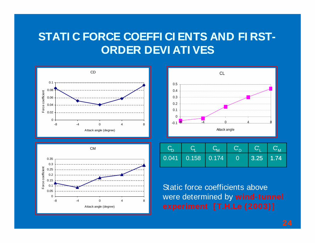
STATIC FORCE COEFFICIENTS AND FIRSTSTATIC FORCE COEFFICIENTS AND FIRST--ORDER DEVIATIVESORDER DEVIATIVES
CD
0
0.02
0.04
0.06
0.08
0.1
-8 -4 0 4 8
Attack angle (degree)
Forc
e co
effic
ient
CL
-0.1
0
0.1
0.2
0.3
0.4
0.5
-8 -4 0 4 8
Attack angle
CM
0
0.05
0.1
0.15
0.2
0.25
0.3
0.35
-8 -4 0 4 8
Attack angle (degree)
Forc
e co
effic
ient
CD CL CM C’D C’L C’M0.041 0.158 0.174 0 3.253.25 1.741.74
Static force coefficients above were determined by wind-tunnel experiment [T.H.Le (2003)]
24
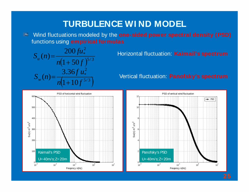
TURBULENCE WIND MODELTURBULENCE WIND MODEL
10-3
10-2
10-1
100
101
0
100
200
300
400
500
600PSD of horizontal wind fluctuation
Freqency n(Hz)
Su(
n) m
2 .s/s
2
Kaimal's spectrumU= 40m/sZ= 20mu*= 2.5m/s
Wind fluctuations modeled by the one-sided power spectral density (PSD)functions using empirical formulas
3/5
2*
501200)(
fnfunSu
3/5
2*
10136.3)(
fnufnSw
Horizontal fluctuation: Kaimail’s spectrum
Vertical fluctuation: Panofsky’s spectrum
10-3
10-2
10-1
100
101
0
2
4
6
8
10
12PSD of vertical wind fluctuation
Freqency n(Hz)
Sw
(n) m
2 .s/s
2
PSD
Kaimal's spectrumU= 40m/sZ= 20mu*= 2.5m/s
Kaimail’s PSD
U=40m/s;Z=20m
Panofsky’s PSD
U=40m/s;Z=20m
25

AERODYNAMIC ADMITTANCEAERODYNAMIC ADMITTANCE
Approximated by well-known Liepmann’s function (1952)
UBn
ni
i 22
21
1)(
ni: Modal frequency
10-2 10-1 100 1010
0.1
0.2
0.3
0.4
0.5
0.6
0.7
0.8
0.9
Frequency Log(n)
Aer
odyn
amic
adm
ittan
ce
B=14.5m; U=40m/s
26

COHERENCE FUNCTIONCOHERENCE FUNCTIONProposed by Davenport (1962) with assumption that coherence of buffeting forces exhibits equal to that of ongoing velocity
)exp(),(U
xcnxnCoh i
iu
C: Decay coefficient (8c16)
x: Spanwise separation
10-2 10-1 100 1010
0.1
0.2
0.3
0.4
0.5
0.6
0.7
0.8
0.9
1
Frequency Log(n)
Coh
eren
ce
y=0.1m
y=0.3
y=0.5
y=1
y=5
y=10
y=30
c=10; x=0.1-30m
x=6m
27

JOINT ACCEPTANCE FUNCTIONJOINT ACCEPTANCE FUNCTION
N
knksmkrkrmsn LG
1,, )()(
Joint acceptance function can be computed by following formulas
dxdxxrxrU
xcnnxxJ
L
BiAih
L
hBAF
00
2 )()()exp(|),,(|
iihhh
hL GxU
xcnnxJ ))(exp(|),(| 2
Discretization
ii ppp
pD GxU
xcnnxJ ))(exp(|),(| 2
iiGx
UxcnnxJ M
))(exp(|),(| 2
i: The number of modeF=L, D or Mr=h, p or
: Modal sum coefficients
mkr )( , : Modal value
Lk: Spanwise separation
28
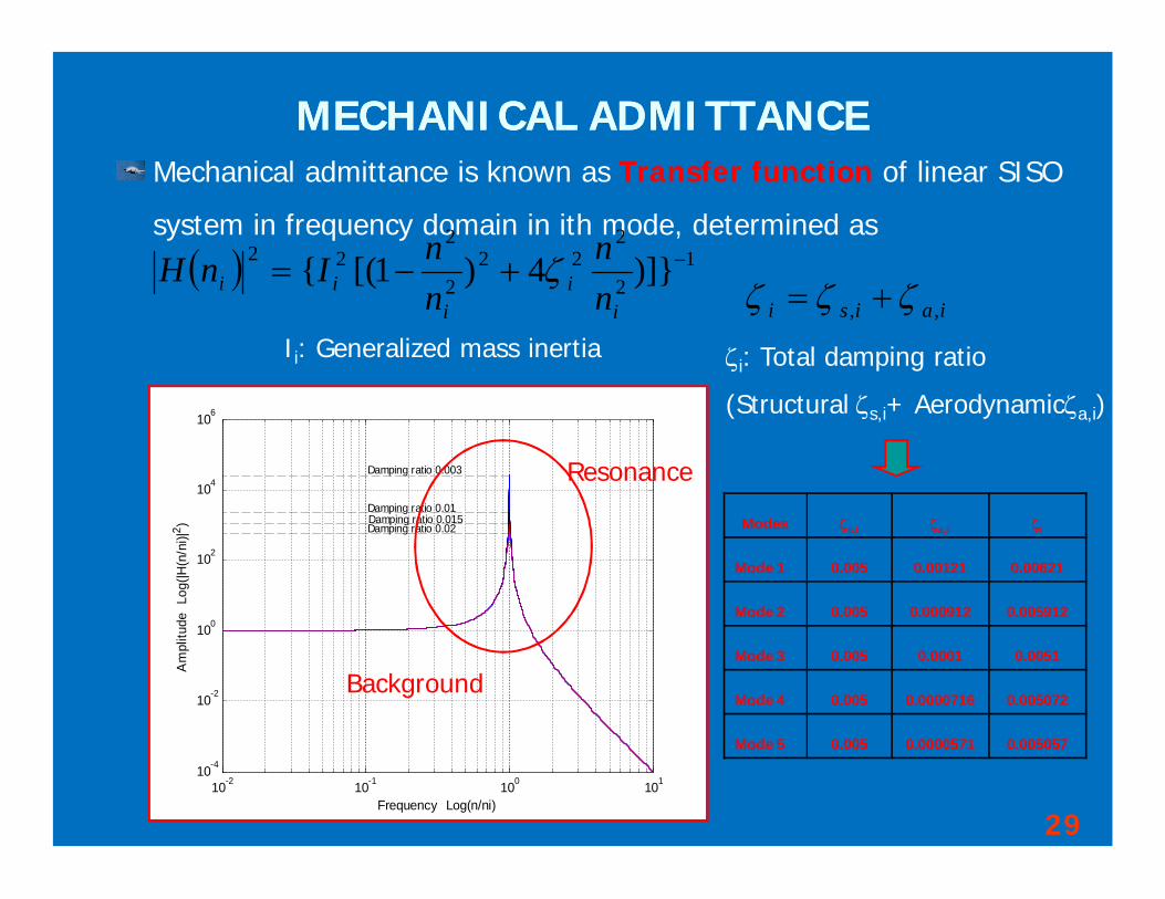
MECHANICAL ADMITTANCEMECHANICAL ADMITTANCE
10-2 10-1 100 10110-4
10-2
100
102
104
106
Frequency Log(n/ni)
Am
plitu
de L
og(|H
(n/n
i)|2 )
Damping ratio 0.003
Damping ratio 0.01 Damping ratio 0.015 Damping ratio 0.02
Mechanical admittance is known as Transfer function of linear SISO
system in frequency domain in ith mode, determined as
12
222
2
222 )]}4)1[({
ii
iii n
nnnInH
Ii: Generalized mass inertia iaisi ,,
i: Total damping ratio
(Structural s,i+ Aerodynamica,i)
29
Modes s,i a,i i
Mode 1 0.005 0.00121 0.00621
Mode 2 0.005 0.000912 0.005912
Mode 3 0.005 0.0001 0.0051
Mode 4 0.005 0.0000716 0.005072
Mode 5 0.005 0.0000571 0.005057
Resonance
Background
30
00.10.20.30.40.50.60.70.8
10 20 30 40 50 60
Mean wind velocity U(m/s)
RM
S of
Rot
atio
n(D
egre
e)
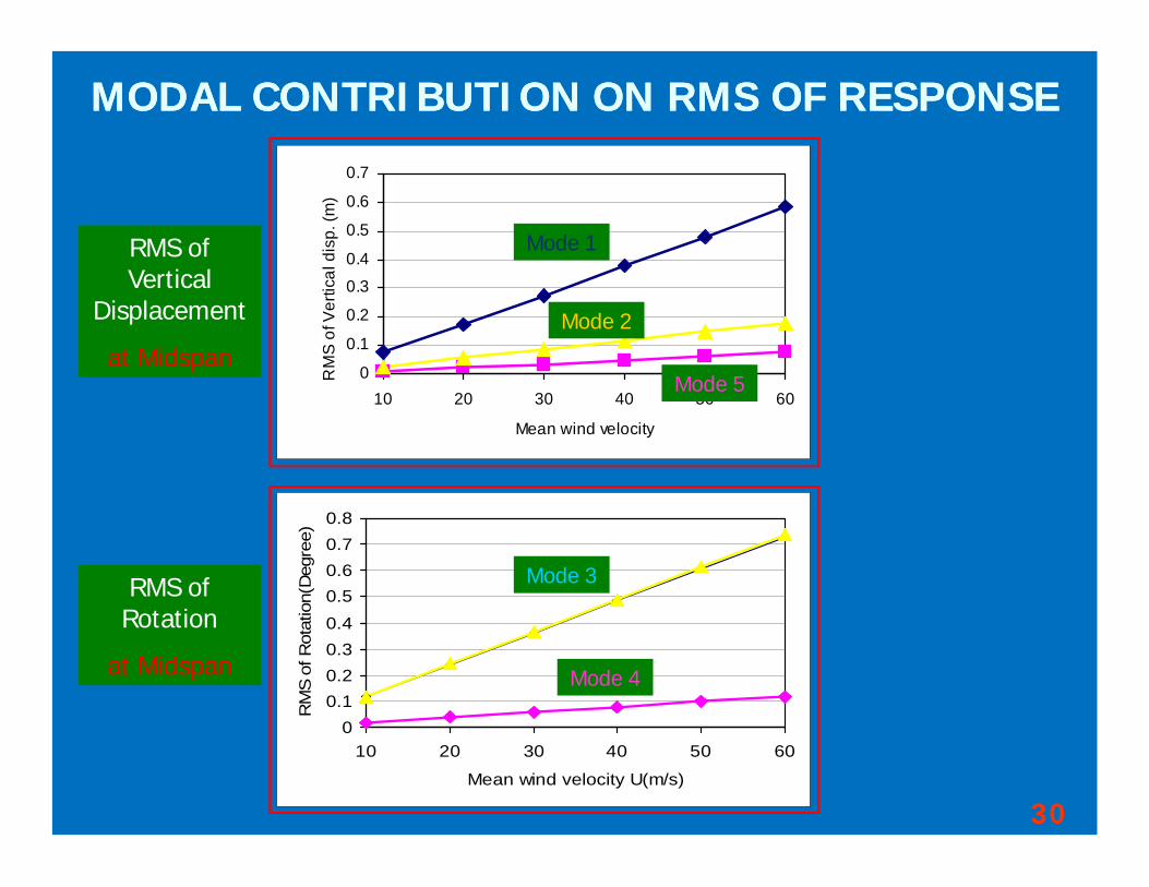
RMS of Rotation
at Midspan
MODAL CONTRIBUTION ON RMS OF RESPONSE MODAL CONTRIBUTION ON RMS OF RESPONSE
0
0.1
0.2
0.3
0.4
0.5
0.6
0.7
10 20 30 40 50 60
Mean wind velocity
RM
S of
Ver
tical
dis
p. (m
)
RMS of Vertical
Displacement
at Midspan
Mode 3
Mode 4
Mode 1
Mode 2
Mode 5

31
RMS OF TOTAL RESPONSE (5 MODES COMBINED)RMS OF TOTAL RESPONSE (5 MODES COMBINED)
RMS of total response (m)
00.10.20.30.40.50.60.7
10 20 30 40 50 60
Mean wind velocity U(m/s)
RMS of Total response (Degree)
0
0.2
0.4
0.6
0.8
10 20 30 40 50 60
Mean wind velocity U(m/s)
RMS of Vertical
Displacement
at Midspan
RMS of Rotation
at Midspan
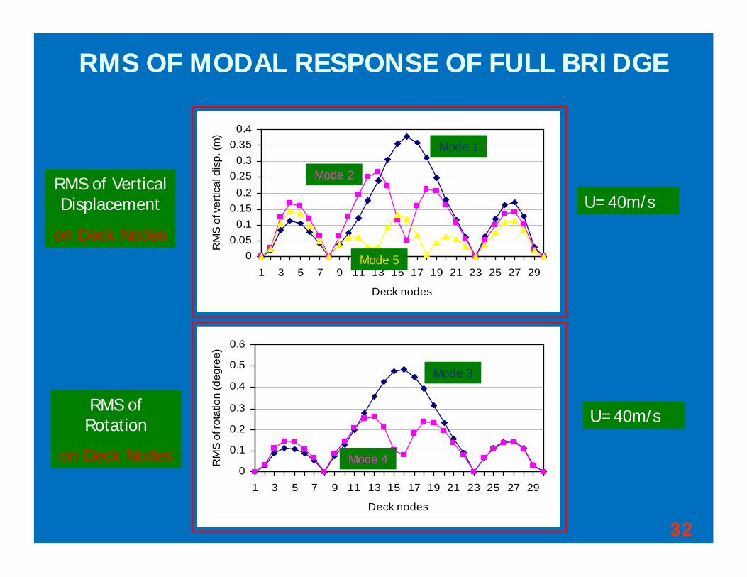
RMS OF MODAL RESPONSE OF FULL BRIDGERMS OF MODAL RESPONSE OF FULL BRIDGE
0
0.1
0.2
0.3
0.4
0.5
0.6
1 3 5 7 9 11 13 15 17 19 21 23 25 27 29
Deck nodes
RM
S of
rota
tion
(deg
ree)
00.05
0.10.15
0.20.25
0.30.35
0.4
1 3 5 7 9 11 13 15 17 19 21 23 25 27 29
Deck nodes
RM
S o
f ver
tical
dis
p. (m
)
RMS of Vertical Displacement
on Deck Nodes
RMS of Rotation
on Deck Nodes
Mode 1
Mode 2
Mode 5
Mode 3
Mode 4
32
U=40m/s
U=40m/s

33
CONCLUSIONCONCLUSION
Some further studies on buffeting vibration and response prediction
will be focused on
(1) Contribution of background and resonance components
to total structural response
(2) Buffeting analysis method in time domain
(Main research point)

THANKS VERY MUCH FOR YOUR ATTENTIONTHANKS VERY MUCH FOR YOUR ATTENTION
Top Related