


Languages
Pages
Legal


waterVaR and waterBeta are trademarks of Water Risk Analytics, all rights reserved; © Water Risk Analytics- used with permission. Patent-pending
Bridging Physical and Financial Business Water Risk: waterVaR and waterBeta Metrics for Equity and Portfolio Risk Assessment
Peter Adriaens1,2,3, Kristine Sun4, and Ran Gao2
1Ross School of Business, 2Civil and Environmental Engineering, and 3School for Natural Resources and Environment; 4Mathematics, The University of Michigan
Peter Adriaens Zell-Lurie Institute for Entrepreneurial Studies Ross School of Business 710 Tappan St, Ann Arbor MI 48109 Kristine Sun Department of Mathematics – Financial and Actuarial Program 2074 East Hall 530 Church Street Ann Arbor, MI 48109-1043 Ran Gao Department of Civil and Environmental Engineering 1351 Beal Ave, Ann Arbor, MI 48109 Corresponding author: [email protected]
2
Abstract The impact of water as a constrained resource for business operations is becoming part of the investor
discourse on equity water risk. A key challenge is the absence of metrics that relate physical risk to
financial risk, either at the company or at the portfolio level, resulting in the lack of asset risk pricing.
Our research tests the hypothesis that water risk impacts revenue and the cost of doing business and, by
inference stock volatility, unless the company manages its risk appropriately. We related stock volatility
metrics and water risk exposures of four electric utilities during a two-year period (2007-2008) that
captured multiple drought events, commodity (coal) price fluctuations, and systemic risk in the financial
markets. Using waterBeta and waterVaR metrics, the impact of water risk on stock volatility (VaR) was
highly dependent on the value chain position of the firm, the capital efficiency of water, and stock
elasticity. The waterVaR values were calculated to range from $5M for the Southern Company to $167M
for AES, accounting for 1-18% of VaR. This range was very similar to the risk management expenditures
by the companies during the summer months ($20-95M). Portfolio VaR and waterVaR analytics
indicated a strong correlation between minimum VaR portfolio performance and lower waterVaR values,
showing that financial risk metrics for water can improve decisions for asset allocation to reduce water
risk exposure in portfolios, including stranded assets.
Keywords: risk management, portfolio volatility, value-at-risk
I. Introduction
The impact of corporate and investor exposures to physical, regulatory and reputational risks from water
has been debated for the last five years, from both a supply-side and demand-side perspective. Indeed,
both academics and policymakers discuss how water planners will need to adopt a variety of adaptation
practices, designed to better conserve our water supplies, improve water recycling, and develop
alternative strategies for water management to meet the needs of growing communities, sensitive

3
ecosystems, farmers, ranchers, energy producers, and manufacturers. The focus on local government
practices for water planning has led to a one-sided argument on supply-side economics and water pricing,
while ignoring demand-side opportunity cost, market risk impacts resulting from volatility in equity
pricing, and the use of market signals to inform investment in (financial) risk management strategies
(Larson et al., 2012).
Water scarcity, water quality, and thermal events are imposing financial risks to water-intensive
companies and agricultural operations, and thus water constraints become liabilities unless they are
properly managed and valued. Business organizations, NGOs, and the financial services industry have
taken note of these risks as they impact economic development, job creation, and shareholder value.
From food and beverage industries to manufacturing and oil & gas production, industry sector
performance is dependent on freshwater access. The materiality of this risk is substantial. For example, a
recent report on the value at risk (VaR0.5) from stranded assets due to resource constraints (including
water) estimated a potential increase from $6.7 trn. to $11.2 trn. (Caldecott et al., 2013). Stranded assets
are environmentally unsustainable assets impacted by unanticipated or premature write-offs, downward
revaluations or are converted to liabilities, as the result to exposure to environment-related risks.
Understanding the financial materiality of water risks facing watershed users cannot be
understood from current industrial ecology frameworks or from water transfer econometrics alone.
Rather, corporate approaches to water sustainability require an understanding of how financial risk
management works, and of how risk mitigation strategies are valued by the market (public firms) or by
private equity investors (private companies).
With the exception of recent academic research, and white papers from non-governmental (e.g.
Ceres, Water Disclosure Project) and accounting organizations (e.g. Deloitte, PWC), corporate water risk
assessment is still largely under the radar for equity analysts, even if it has risen to the level of the Chief
Financial Officer in the corporate organization. Yet, given the material risk of water to revenue, stock
prices, and asset valuation, the corporate and investor focus on water strategies is increasingly germane to
4
the sustainability discussion. A number of tools have been developed by the financial services industry
and non-governmental organizations to take into account water risk to businesses.
For example, the World Wildlife Fund (WWF) and DEG (a German bank) have partnered to
develop a ‘water risk filter’, based on a suite of basin- and company-related indicators that embed outputs
from hydrological modeling. Company-related risk indicators include how much withdrawn freshwater is
discharged with a certain type of pollution, the company’s exposure to regulatory changes, and its
contingency planning around supply disruptions, price increases and more stringent regulations. Basin-
related risk indicators include total annual renewable freshwater resources per capita and questions
regarding enforcement of water-related regulations in the river basin in which the company is operating
(WWF, 2011). The World Resources Institute (WRI), in partnership with industrial partners and academic
advisors, has developed a navigable water risk map (Aqueduct), focused on comprehensive metrics for
measuring geographic business water risks. The Aqueduct project consists of a global database and
interactive tool that enable companies to quantify and map water risks at a local scale, worldwide.
II. Corporate Water Risk Management
1. Risk management approaches.
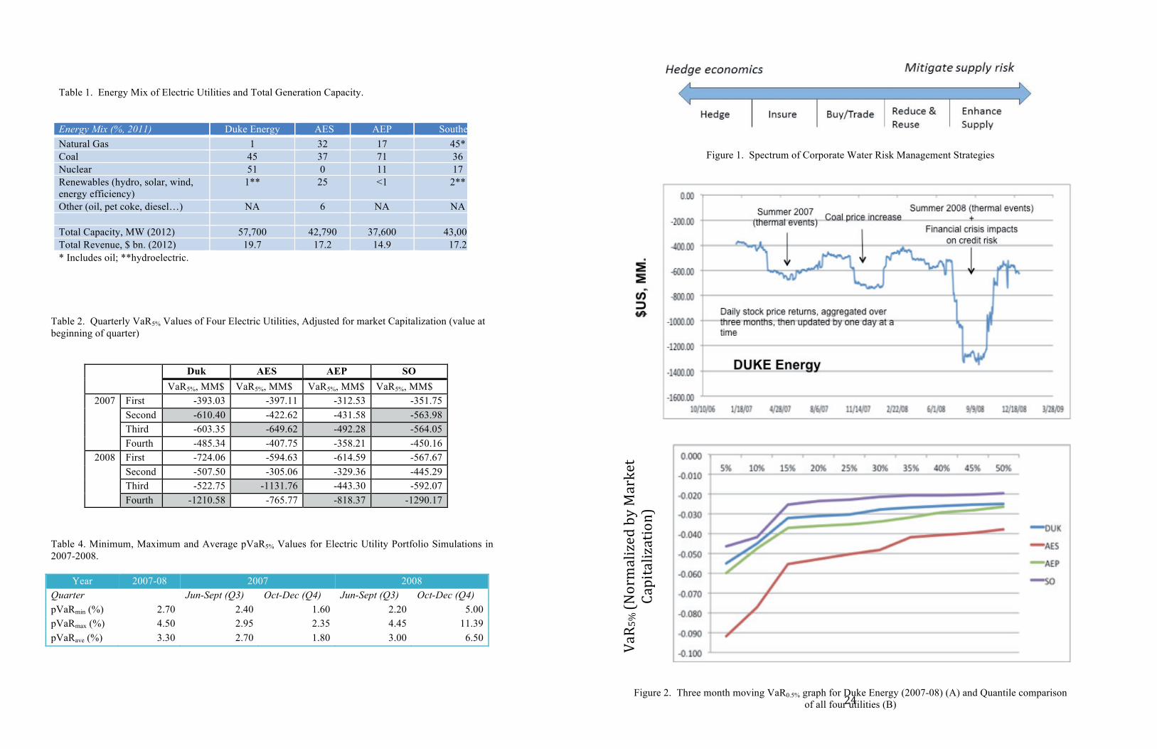
Corporations avail themselves of several tools to offset water risk exposure, including hedging strategies,
real options, derivatives or insurance contracts, water trades, and infrastructure investment (Larson et al.,
2012). Investments for water efficiency and reuse technologies, water supply enhancements (pipelines,
desalinization plants, etc), and investments in real assets, are treated as long-term capital asset
expenditures. Hedging strategies, risk transfer tools (insurance), and water trades tend to be short-term
risk management tools that are more flexible.
Figure 1 about here

5
Depending on the industry sector under consideration (e.g. energy, mining, food and beverage,
etc..), differences tend to exist in the mix of risk management approaches used by corporations. For
example, electric utilities facing de-rating events (production of less than nameplate capacity power) have
the option to lock in pricing on the open market or increase production at secondary plants. The
reduction of water use through investment in cooling towers, or investment in make-up power through
alternative energy production (e.g. wind or solar energy) represent major infrastructure investments that,
while accomplishing the goal of reduced water use, can negatively impact operational costs and profits,
and thus impact stock volatility. The rationale is that unless the investment can be passed on to the
consumer, major investments in water risk management by companies operating in a regulated sector (e.g.
electric utilities, water utilities) will be deferred unless rate structures are renegotiated. Apparel firms
have been focusing on water efficiency processes in their operations, while food and beverage combine
infrastructure investment with agricultural commodities hedging. Agricultural companies avail
themselves of insurance, hedging positions, and investments in irrigation efficiency infrastructure.
2. Financial Risk Pricing of Water: Water Value-at-Risk (waterVaR).
With corporate water risks manifesting themselves both at the watershed and corporate governance level,
investment decision-making has to be informed by a valuation of the opportunity cost of the impacted
industry [e.g. Barth et al., 1997; Blacconiere and Northcut, 1997; McKinsey, 2009]. From a corporate
perspective, the economic value of the risk management options is typically evaluated using net present
value, discounted cash flow, or real options analysis to compare investments on a return-basis [e.g.
Clarkson et al., 2004]. The term “real options” is commonly used in the context of strategic corporate
planning when faced with decision-making under uncertainty [Heal, 2005]. The uncertainties associated
with water risks, allocation policies, and water pricing present a challenge for investment decisions by the
relevant industries (e.g. oil & gas, utilities, mining, beverage and apparel, e.g. [Bauer and Hann, 2010]).
Hence, the decision of the firm to, for example, buy insurance vs. invest in water supply infrastructure, is
one of capital efficiency in the face of uncertain future cash flows.
6
In the financial markets, risk ‘pricing’ of assets has long been an aspiration for equity analysts
and portfolio managers to capture sensitivities of asset value to systematic (market) risk and residual
(company-specific or idiosyncratic) risk. Water risk exposures, and the strategies employed to offset the
risk impacts to business operations, are considered a systematic risk, while company-specific impacts
represent idiosyncratic risks. The underlying premise is that there is a relationship between the risk driver
and the return-on-equity (ROE) or return-on-assets (ROA). Similarly, the voluntary water risk
disclosures under Sarbanes-Oxley are only ‘material’ if the water risk (and risk mitigation strategies can
be tied to returns (and thus revenue targets or asset valuation). To date, specific risk-pricing strategies
pertaining to water scarcity, climate change, or environmental, social and governance (ESG) risks have
not been attempted. Rather, investors use simplifying assumptions such as the market risk measurement β
(beta), a dimensionless ratio that captures deviations of a firm’s performance from the market
performance in a given industry. The impact of ESG performance can then be integrated as a weighting
factor influencing the β value.
The challenge with using a simplifying ‘beta’ is that this metric exhibits tenuous predictive
capacity to securities returns. In other words, they need to be informed by robust understanding of
underlying risk data. An approach that is widely used in the financial services industry is the value-at-risk
(VaR) model [Jorion, 2007; Rockefeller and Uryasev, 2002]. At the conceptual level, the VaR model is a
probabilistic metric that takes into account the likelihood of an event occurring that will impact the value
of a given portfolio of companies (say, exposure to water risks such as drought, temperature, quality, etc)
[Innovest, 2002; Webby et al., 2007]. The probabilistic element of VaR is that it quantifies the losses of a
stock or portfolio performance at various levels of confidence (e.g. 0.1%, 1%, 5%). For example,
suppose a $1 MM. portfolio of stocks of companies is potentially exposed to water risk, and the
probability of risk is normally distributed with an intra-day standard deviation of 100 base points (bp) on
the stock value. For any normally distributed random variable, there is a 5 percent chance that an
observation will be less than 1.645 standard deviations below the mean. Or, using the properties of the
normal distribution, the 5 percent chance that the value will decline by more than 1.645 × 100 bp =
7
1.645%. Based on the $1 MM. equity portfolio in the example, this represents a minimum daily loss of
$16,450 (0.01645 × $1 MM.), which will be exceeded only 5 percent of the time. Thus, the equity VaR5%
on a $1 MM. portfolio is $16,450.
The ability to value water risk using financial metrics used in capital markets presumes that water
risk has a material impact on (and thus is related to) revenue, production cost, and financial ROA or ROE.
The ROA conveys what a company can do with what it has, i.e. how many dollars of earnings they derive
from each dollar of assets they control. The ROE, on the other hand, shows how well a company uses
investment funds to generate earnings growth and is shareholder-oriented. To demonstrate material
impact, information is required on: (i) the impact of water quality and quantity on the company’s
operations; (ii) what the company does to mitigate this risk (hedge, insure, water banking, infrastructure
investment); and (iii) whether the risk management strategy reduces financial risk (operational or as the
result of asset valuation shifts) to the firm.
The probabilistic understanding of these relationships provides the theoretical backbone for the
development of a financial water-based VaR metric. This VaR derivative, the waterVaR™, quantifies the
water-based liability as part of this volatility. The premise is that this represents a market signal for water
risk valuation (pricing) of companies and portfolios.
The focus of this paper is to demonstrate the application of waterVaR™ and waterBeta™ risk
metrics for four electric utilities in the Southeastern US, and to start developing portfolio-based risk
metrics for a simulated investment portfolio that holds these companies.
III. Methods
1. Companies.
The project focused on four electric utilities with operations predominantly in the South-Eastern and Mid-
Western US. The companies, Duke Energy, AES, American Electric Power (AEP), and the Southern
Company, were chosen based on water risk disclosures and availability of water intensity data through the
8
CDP database (CDP Water Disclosure program, London, UK), or imputed values from SEC disclosures
and sustainability reports. Whereas Duke Energy and AEP are companies with regional operations, AES
is a global corporation with operations in 27 countries, predominantly in the US and Latin America, and
the Southern Company is structured as a holding company with assets across several regions. Each
company’s generation mix and total capacity are shown in Table 1.
The data indicate that AES is the only electric utility among the four companies that does not
have nuclear energy in its mix, and has a predominant proportion of renewable energy in its portfolio
(predominantly hydro). Southern Company has the highest proportion of natural gas in its mix, and Duke
Energy has the highest proportion of nuclear energy.
Table 1 about here
2. Value at Risk (VaR) Calculations.
The VaR5% metrics are industry- and company- specific as they reflect how capital markets view and
reward risk management strategies. Two VaR metrics were calculated: (i) the three month moving
VaR5%, computed over a 90-day period, but adjusted on a daily basis over the two year time horizon
studied in this report (2007-08); (ii) the VaR5% calculated based on quarterly reporting periods. Inclusion
of the longer time horizon allows for uncovering VaR trends as a function of seasonal impacts and to
uncover systemic risk impacts. Briefly, daily stock returns were downloaded from Bloomberg terminals
to calculate daily returns. These were then plotted on a quarterly basis, and over two years. The current
paper focuses on the 2007-2009 period because of the availability of risk management strategy data, and
the coverage of two major drought events. Both market capitalization-adjusted and absolute VaR metrics
are reported. The calculated VaRs of the different companies can be compared by plotting the VaR5%
quantiles as a cumulative distribution function (cdf). This allows for groupings of companies in
accordance with their VaR behavior: the flatter the cdf the less volatile the stock. Three month moving

9
VaR5% data help with focusing on the specific time periods during which ‘drought events’ may have an
impact on stock performance.
The quarterly VaR5% calculations focused on the time periods selected based on the two-year
VaR where the company was most volatile, and when specific weather, temperature or drought events
were known to occur. The objective was to capture the financial reporting quarter with the largest VaR
values (VaR5%,max) during these periods (systemic + idiosyncratic or company-specific risk) and correct
them for systemic risk impacting this industry sector, based on average VaR data for the remaining three
reporting quarters (VaR5%,ave). Hence,
ΔVaR5% = VaR5%,max – VaR5%,ave (1)
3. Revenue Sensitivity to Water (waterBeta™) Calculations.
The rationale for structuring a waterBeta is to allow for inter-sector and cross-sector comparisons of
company revenue sensitivity when compared to a benchmark (e.g. companies operating on a specific
watershed or basin, companies with similar industry classification codes, or the market as a whole). This
metric is defined as a dimensionless sensitivity ratio. WaterBeta™ values are thus an indicator of
sensitivity of revenue to water availability, and the ratio is based on a water exposure metric termed
‘capital efficiency of water’ (CEw; water withdrawal/revenue). Similar key water risk metrics of a
company are currently in use: water intensity (WI, water use/unit produced), and financial intensity (FI,
revenue/water use). Financial intensity can be either based on water withdrawals or water use in process.
The CEw defined here is the inverse of financial intensity, and is specific to water withdrawals as a proxy
of overall water availability. The denominator of CEw calculations is specific to revenue generation from
energy production (to avoid inclusion of different lines of business unrelated to energy generation).
The CEw of the benchmark is based on the reference chosen. In the case of this paper, the
reference is the aggregate value of all four companies in the portfolio.
10
waterBeta™ = CEw (company)/CEw (benchmark) (2)
The interpretation of the waterBeta™ is that a company can be less financially sensitive, similarly
sensitive or more sensitive than the benchmark average. To correct for the relative share price movement
of a given stock relative to the broader market in response to risk exposures, the waterBeta™ is corrected
for the reported company Beta. The boundary condition is that the waterBeta values can't be greater than
unity because in that case the waterVaR™ would exceed the overall equity VaR of that quarter, which is
impossible. The waterVaR™, defined as the opportunity cost from water risk exposures that may impact
equity and portfolio volatility, is then calculated as a product of the waterBeta™ and the VaR differential
(based on quarterly stock price volatility).
waterVaR5% = waterBeta x [VaR5%,max-VaR5%,ave] (3)
To validate the magnitude of waterVaR values, company-specific information is required on the
investment in water risk management strategies, because they are a proxy for the company’s opportunity
cost due to water risk. Often, information at this level of specificity is not publicly disclosed in corporate
financial disclosures, or is even not known, and thus has to be inferred. An example will be provided on
an electric utility’s investment in hedging strategies (open market positions and cost to increase
production at a secondary plant) to offset water risks during the summer months. It should be noted that
even though water risks and regional opportunity costs from water have been calculated or estimated (e.g.
Hoekstra and Mekonnen, 2011; MSCI, 2013; Rice, 2010), the relationship of water risk exposures to
financial risk volatility (‘risk pricing’) in the market has to date not been attempted.
4. Portfolio Simulations.
11
To assess the effect constituent companies have on the volatility of a hypothetical portfolio of these four
stocks (DUKE, AES, AEP, SO), 100 simulated allocations were conducted to estimate minimum,
maximum, and average portfolio VaR5% values. To estimate portfolio VaR values, a covariance matrix is
constructed using independent stock price returns for the four utility companies during the period under
consideration (e.g. 2007 or 2008). The variance of a portfolio's return is a function of the variance of the
component assets (the four utilities stock returns) as well as the covariance between each of them.
Covariance is a measure of the degree to which returns on two assets move in tandem. A positive
covariance means that asset returns move together. A negative covariance means returns move inversely.
It should be noted that proper portfolio designs minimize covariance between the stocks to spread the
risk. In this study, the objective was not to structure an investable portfolio, but rather to evaluate how
individual company risk volatility impacts a grouping of these stocks.
Portfolio variance, the covariance or correlation coefficient for the stocks in the portfolio, was
calculated in excel for each allocation (= allocation of stocks * covariance matrix in a portfolio *
allocation of stocks). Portfolio returns were assumed normally distributed, and the
maximum/minimum/average portfolioVaR (pVaR) was calculated for all 100 simulations over 2 years, on
a quarterly basis. The pVaR5%,min is represents a portfolio allocation with lowest possible VaR volatility,
while, conversely, the pVaR5%,max is based on a stock allocation with highest portfolio volatility. By
bracketing the extreme values, it is possible to discern which stock influences the volatility most (least).
The portfolio waterVaR was calculated based on the company allocations that led to the pVaR5%,max and
pVaR5%, min, multiplied by their waterBeta™ values.
IV. Results
The water risk impact results are presented in the context of financial risk of the utilities in the market.
Hence, the stock volatility trends will be presented first to understand the magnitude of long term and
quarterly losses, and how these losses correspond to key events. The impact of stock volatility on
portfolio variance and VaR5% will be discussed from the perspective of identifying which companies have
12
a stabilizing or destabilizing effect on the volatility, and how this impacts stock allocations. The
connection to the physical world of water is accomplished by way of understanding the sensitivities of
revenue to water disruptions, and their impact on potential opportunity costs as reflected in waterVaR™
losses.
1. Electric Utility Stock Volatility Trends
The three-month VaR5% was plotted for each company over the 2007-2008 timeframe to identify periods
of significant volatility (loss) events. This is exemplified for Duke Energy (Figure 2, A), where the plot
shows that these events coincide with summer months when drought and thermal events influence energy
output. In addition, significant contributions to the losses were influenced by fuel (coal) price increases,
affecting the cost of generation. This is not surprising given the dependency of these utilities on coal,
being 37-71% of their energy mix. Similar plots and trends were apparent for the other three utilities
(data not shown), with differences in the depth of the troughs in the data.
Given that equity VaR volatility encompasses the security’s market pricing in response to
financial performance, commodity price fluctuations, and externalities such as ESG issues, it is very
challenging to tease out the specific contributions of each factor. However, the seasonality of extreme
losses may be indicative of the contribution of weather and other environmental (water-related) events.
Indeed, data from voluntary CDP disclosures (for Duke, AEP and Southern) and Global Reporting
Initiative (GRI) reports, as well as a review of mandatory SEC disclosures (Adrio, 2012), lend credence to
the impact water is starting to have these companies. For example, as will be shown later, the capital
efficiency of water (CEw), which measures the sensitivity of revenue to water withdrawals, has been
increasing since 2008 in the case of The Southern Company and AES, and fluctuating in the case of Duke
and AEP. This occurring even as total water withdrawals are decreasing as the result of investments in
water efficiency (e.g. cooling towers) and energy mix diversification, which comes at a cost to the
company. Since these costs can’t be easily recaptured in regulated markets (unless a change in ratepayer
restructuring is approved), the markets perceive this investment as an increase in the cost of doing
13
business, resulting in a (temporary) down-valuation of the stock. In addition, NGOs have filed water risk
management disclosure information from electric utilities in the South-Eastern US on behalf of
shareholders, indicating that the impact of water on share price is perceived to be significant, and needs to
be addressed.
Cumulative distribution functions (cdf) of the 3-month moving VaR5% values allow for a
comparison of the volatility losses among the four stocks (Figure 2, B). The figure, which plots percent
occurrence of the loss against the magnitude of the loss, shows that, even if the VaR plots may indicate
similar behavior in financial risk, the distribution of these losses is quite different. It should be noted that,
to compare VaR losses for different companies, it is important to normalize the loss by market
capitalization. Following this normalization, the Southern Company’s financial performance is least
volatile during this two-year period, followed by Duke, AEP and AES. The relative response of stock
returns and 5% extreme losses in a period encompassing multiple drought periods is significant in the
assessment of quarterly VAR evaluations, and the impact of revenue sensitivity to water.
Figure 2 about here
Quarterly (90 day) VaR5% losses were calculated for the eight financial reporting periods
(quarters) and for all four companies (Table 2). The objective was to isolate the impact of weather and
temperature events on VaR5% losses, by employing statistical metrics such as skewness and kurtosis on
distribution of the 90-day returns. Operational VaR losses from weather or environmental events tend to
exhibit the following characteristics: they are short-term, have high kurtosis (‘sharp peaks’), and long tails
in the distribution. Applying these criteria to the VaR distributions, the summer of 2007 noted VaRmax
values in the 2nd and 3rd quarter, corresponding to the March-June timeframe of the first dip in the 3-
month VaR5% (Figure 2, A). Similarly, in 2008, the VaR5%,max was predominant in the 4th quarter (except
for AES), corresponding to an August-late November dip in the 3-month VaR5% returns (Figure 2, A).
14
Table 2 about here
For demonstration purposes in this paper, the focus of the water risk impacts on stock returns and
VaR was on the third quarter of 2007 and the fourth quarter of 2008 where drought events were known to
occur (and impact volatility). As stated earlier, even though there was correspondence between the
VaR5%, max and the extreme losses during drought and thermal event periods, there are many factors that
influence the volatility of securities. Hence, an attempt was made to isolate idiosyncratic (company- or
event-specific) volatility from systemic (broader market trends that impact stocks) volatility. This was
accomplished by averaging the VaR5% of all quarters, and subtracting this from the VaR5%,max with left
skewed distributions. These values will be discussed as part of the waterVaR™ section.
2. Electric Utility waterBeta™ and waterVaR™ trends
Electric utilities, like many other public companies have started to disclose their water risk exposures and
water risk management strategies via forums such as CDPs Water Disclosure Project and SEC filings.
When compared on a water intensity (water use v. production) and financial intensity (revenue generated
v. total water use) basis, Figure 3 indicates that Duke Energy has the highest dependency on water for its
electrical output, nearly an order of magnitude higher than the Southern Company. Since water intensity
includes water use, and not just withdrawals, Duke’s energy mix driven by nuclear and coal is largely
responsible for it differentiation from the other utilities. AEP is the most water-efficient company in
terms of revenue generation (financial intensity), though all electric utilities are within a 20% range,
indicating similar dependency on water to generate revenue. The waterBeta™ (unitless), which describes
the ratio of the company CEw to the sector CEw, and thus indicates the influence of water constraints on
revenue relative to the sector (Figure 4), shows that AES is most sensitive (highest waterBeta) and the
Southern Company least sensitive (lowest waterBeta) to water risk exposure. The Beta and waterBeta
move generally in the same direction, and trend similarly. However, AEPs waterBeta is higher than its
15
Beta, indicating exacerbated price sensitivity due to water risk exposures. On the other hand, the impact
of water risk exposure on AES effects less stock price elasticity than that of overall market risk exposures.
Figure 3 about here
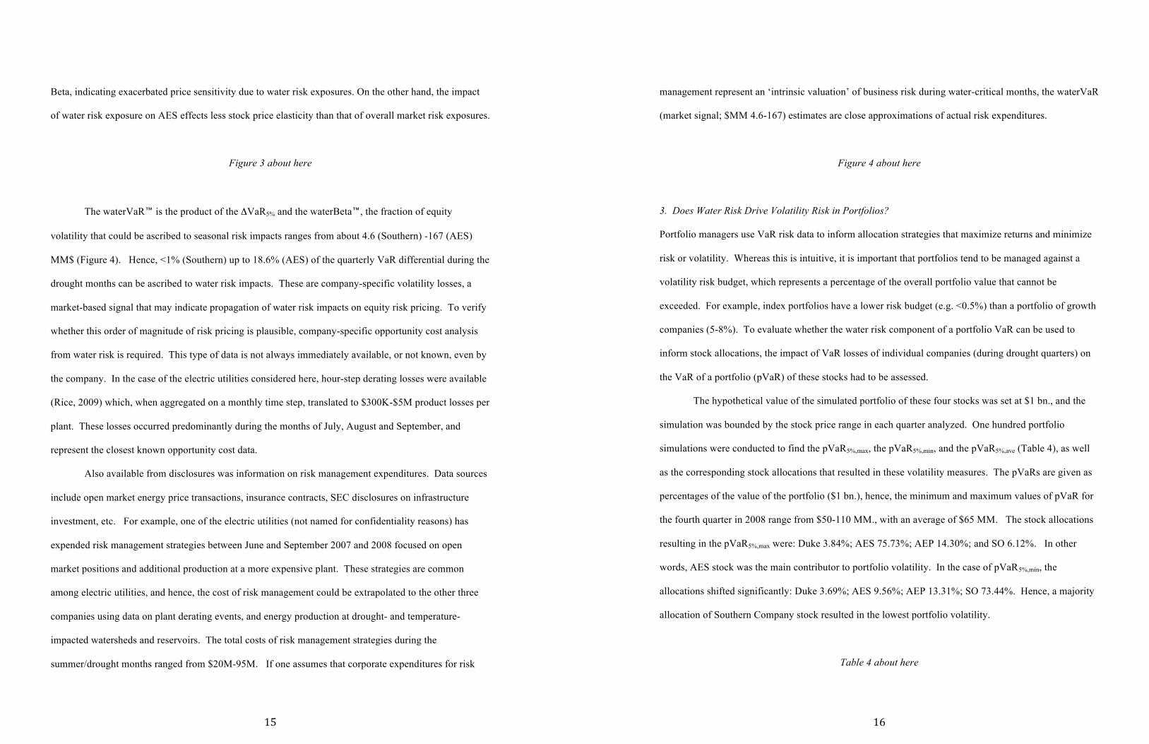
The waterVaR™ is the product of the ΔVaR5% and the waterBeta™, the fraction of equity
volatility that could be ascribed to seasonal risk impacts ranges from about 4.6 (Southern) -167 (AES)
MM$ (Figure 4). Hence, <1% (Southern) up to 18.6% (AES) of the quarterly VaR differential during the
drought months can be ascribed to water risk impacts. These are company-specific volatility losses, a
market-based signal that may indicate propagation of water risk impacts on equity risk pricing. To verify
whether this order of magnitude of risk pricing is plausible, company-specific opportunity cost analysis
from water risk is required. This type of data is not always immediately available, or not known, even by
the company. In the case of the electric utilities considered here, hour-step derating losses were available
(Rice, 2009) which, when aggregated on a monthly time step, translated to $300K-$5M product losses per
plant. These losses occurred predominantly during the months of July, August and September, and
represent the closest known opportunity cost data.
Also available from disclosures was information on risk management expenditures. Data sources
include open market energy price transactions, insurance contracts, SEC disclosures on infrastructure
investment, etc. For example, one of the electric utilities (not named for confidentiality reasons) has
expended risk management strategies between June and September 2007 and 2008 focused on open
market positions and additional production at a more expensive plant. These strategies are common
among electric utilities, and hence, the cost of risk management could be extrapolated to the other three
companies using data on plant derating events, and energy production at drought- and temperature-
impacted watersheds and reservoirs. The total costs of risk management strategies during the
summer/drought months ranged from $20M-95M. If one assumes that corporate expenditures for risk
16
management represent an ‘intrinsic valuation’ of business risk during water-critical months, the waterVaR
(market signal; $MM 4.6-167) estimates are close approximations of actual risk expenditures.
Figure 4 about here
3. Does Water Risk Drive Volatility Risk in Portfolios?
Portfolio managers use VaR risk data to inform allocation strategies that maximize returns and minimize
risk or volatility. Whereas this is intuitive, it is important that portfolios tend to be managed against a
volatility risk budget, which represents a percentage of the overall portfolio value that cannot be
exceeded. For example, index portfolios have a lower risk budget (e.g. <0.5%) than a portfolio of growth
companies (5-8%). To evaluate whether the water risk component of a portfolio VaR can be used to
inform stock allocations, the impact of VaR losses of individual companies (during drought quarters) on
the VaR of a portfolio (pVaR) of these stocks had to be assessed.
The hypothetical value of the simulated portfolio of these four stocks was set at $1 bn., and the
simulation was bounded by the stock price range in each quarter analyzed. One hundred portfolio
simulations were conducted to find the pVaR5%,max, the pVaR5%,min, and the pVaR5%,ave (Table 4), as well
as the corresponding stock allocations that resulted in these volatility measures. The pVaRs are given as
percentages of the value of the portfolio ($1 bn.), hence, the minimum and maximum values of pVaR for
the fourth quarter in 2008 range from $50-110 MM., with an average of $65 MM. The stock allocations
resulting in the pVaR5%,max were: Duke 3.84%; AES 75.73%; AEP 14.30%; and SO 6.12%. In other
words, AES stock was the main contributor to portfolio volatility. In the case of pVaR5%,min, the
allocations shifted significantly: Duke 3.69%; AES 9.56%; AEP 13.31%; SO 73.44%. Hence, a majority
allocation of Southern Company stock resulted in the lowest portfolio volatility.
Table 4 about here
17
The portfolio-based waterVaR™ is the constituent waterVaR™ based on the stock allocations that
are responsible for either the minimum or maximum volatility in the portfolio. The calculated portfolio
waterVaR for the minimum and maximum pVaR5% allocations was calculated to range from $25-130
MM., a similar range as the actual risk management expenditures by the companies. A comparison of
portfolio waterVaR values to the portfolio VaRmax or VaRmin values is challenging, given that the portfolio
VaR scales as a function of the assumed value of the portfolio. When the calculated portfolio waterVaR
is compared to a $1bn portfolio value, the values represent 2.5-13% of the portfolio value.
Since portfolio waterVaR values are weighted based on stock allocations and individual
waterBeta values, and not derived from deltaVaR values during drought/thermal event-impacted seasonal
events, it is more appropriate to estimate the portfolio waterVaR percent of pVaR based on data fro the
individual companies. It was previously calculated that the waterVaR of individual companies explained
22.6 -36.5 % of the deltaVaR difference between the VaRmax quarter and the average systemic VaR.
Compared to the total 4th quarter VaR in 2008 (Table 2), the waterVaR represents 8.5% (Duke), 8.9%
(Southern), 8.0% (AEP), and 5.1% (AES). Using 5-9% as a benchmark for waterVaR contributions to
VaR, financial water risk impacts constitute an appreciable volatility risk driver in this simulated
portfolio, given that the estimated value of water risk volatility losses during summer are $25-130MM.
Can these market signals be used to inform portfolio asset allocations? Risk-based asset
allocations are feasible if there is a relationship between risk pricing and the underlying risk of the asset.
Closer analysis of the portfolio results indicates that the pVaR and portfolio waterVaR are correlated: the
high pVaR allocation exhibits $130MM. in risk, while the low pVaR allocation results in $25MM.
waterVaR. Indeed, the majority stock in a pVaRmin portfolio is the Southern Company, which also has the
lowest waterBeta and waterVaR. Similarly, the majority stock in the VaRmax portfolio is AES, which was
calculated to have the highest waterBeta and waterVaR. Hence, a increased allocation of Southern or an
decreased allocation of AES, aimed at reducing the water intensity of a portfolio, would also result in
lowering the VaR of the portfolio.
18
V. Conclusions
This paper asked the question whether portfolio allocation decisions can serve as a market signal for
corporate water sustainability. The premise is that business water risk has a measurable and material
impact on equity and portfolio volatility. To prove this hypothesis, the research defined and employed
two measures that leverage public corporate disclosure data: waterBeta and waterVaR. The application
of these tools to electric utilities in the SouthEast indicates that financial volatility of individual
companies and of simulated portfolios tracks risk management expenditures. The work further indicates
that financial water risk represents a significant fraction of the total VaR during drought periods or
thermal events. Given that equity analysts consider 3% of VaR a potential trigger for closer scrutiny, all
but Southern’s waterVaR are material. Given the caveat of this limited sample of companies, asset
allocation decisions based on waterVaR should be carefully interpreted. Southern Company (low
waterVaR) also has a dampening effect on portfolio risk volatility, whereas AES (high waterVaR)
exacerbates pVaR risks. It should be noted that the use of VaR analytics alone is insufficient, because
companies, investors and banks use different time horizons to assess financial risk (e.g. Osborn, 2013).
Larger samples of companies and cross-industry sector applications will help to strengthen the case for
waterBeta and waterVaR approaches to inducing investments in business water risk strategies.
Acknowledgements. PA thanks support from LimnoTech and Water Risk Analytics for this work.
Collaborations with MSCI (NY) and extensive industry discussions with the financial services industry
contributed to contextualizing this work.
VI. References
Barth, M. E., McNichols, M. F., Wilson, P., 1997. Factors influencing firms` disclosures about
environmental liabilities. Review of Accounting Studies 2, 35-64.
Bauer, R. and D. Hann. 2010. Corporate Environmental Management and Credit Risk. SSRN:
http://ssrn.com/abstract=1660470 or http://dx.doi.org/10.2139/ssrn.1660470.

19
Blacconiere, W. G., Northcut, W. D., 1997. Environmental information and market reactions to
environmental legislation. Journal of Accounting. Auditing & Finance 14,149-178.
Adrio, B. 2012. Clearing the Waters: A Review of Corporate Water Risk Disclosure in SEC Filings.
Ceres Report, Creative Commons, San Francisco, CA.
Caldecott, B., N. Howarth, and P. McSharry. 2013. Stranded Assets in Agriculture: Protecting Value
from Environment-Related Risks. White Paper, The Stranded Assets Program at the University of
Oxford’s Smith School of Enterprise and the Environment.
Clarkson, P., Li, Y., and G. Richardson. 2004. The market valuation of environmental capital
expenditures by pulp and paper companies. The Accounting Review 79, 329-353.
Heal, G. 2005. Corporate Social Responsibility: An Economic and Financial Framework, Geneva Papers
30, 387-409.
Hoekstra, A.Y. and Mekonnen, M.M. 2011. Global water scarcity: monthly blue water footprint
compared to blue water availability for the world’s major river basins. Value of Water Research Report
Series No. 53. UNESCO, The Hague, The Netherlands.
Innovest Strategic Value Advisors, Inc. 2002. Value at Risk: Climate Change and the Future of
Governance. The Ceres Group, Boston, MA.
Jorion, P. 2007. Value at Risk: The New Benchmark for Managing Financial Risk. 3rd Edition. 531 pp.
McGraw-Hill, New York, NY.
Larson, W., P. Freedman, and P. Adriaens. 2012. Mitigating Corporate Water Risk: Financial Market
Tools and Supply Management Strategies. Water Alternatives 5(3): 582-602.
McKinsey & Company. 2009. Charting Our Water Future: Economic frameworks to inform decision-
making. 2030 Water Resources Group.
(http://www.mckinsey.com/clientservice/water/charting_our_water_future.aspx)
MSCI 2013. ESG Issue Report: Executive Summary: Water Upstream and Downstream Impacts from a
Well Running Dry. MSCI Inc, NY, NY.
Osborn, T. 2013. Forgetting Lehman. Risk.net/Risk Magazine October 2013, pp. 28-30.
20
Rice, J. 2010. Water Resource Risk and Technology Investment under Uncertainty: A real options
approach to the valuation of water conservation technology at a thermoelectric power plant. M.S.
Thesis, Erb Institute for Global Sustainable Enterprise, The University of Michigan.
Rockefeller, R.T. and S. Uryasev. 2002. Conditional value-at-risk for general loss distributions, Journal of
Banking & Finance 26, 1443-1471.
Webby, R.B., Anderson, P.T., Boland, J., Hewlett, P.G., Metcalfe, A.V. and J. Piantadosi. 2007. The
Mekong—applications of value at risk (VaR) and conditional value at risk (CVaR) simulation to the
benefits, costs and consequences of water resources development in a large river basin. Ecological
Modeling 201 (1): 89-96.
World Wildlife Fund, 2011. Assessing Water Risk: A Practical Approach for Financial Institutions. A
WWF-DEG Report, Washington, DC.
21
Table 1. Energy Mix of Electric Utilities and Total Generation Capacity.
Energy Mix (%, 2011) Duke Energy AES AEP Southern Natural Gas 1 32 17 45* Coal 45 37 71 36 Nuclear 51 0 11 17 Renewables (hydro, solar, wind, energy efficiency)
1** 25 <1 2**
Other (oil, pet coke, diesel…) NA 6 NA NA Total Capacity, MW (2012) 57,700 42,790 37,600 43,000 Total Revenue, $ bn. (2012) 19.7 17.2 14.9 17.2 * Includes oil; **hydroelectric.
22
Table 2. Quarterly VaR5% Values of Four Electric Utilities, Adjusted for market Capitalization (value at beginning of quarter)
Duk AES AEP SO VaR5%, MM$ VaR5%, MM$ VaR5%, MM$ VaR5%, MM$
2007 First -393.03 -397.11 -312.53 -351.75 Second -610.40 -422.62 -431.58 -563.98 Third -603.35 -649.62 -492.28 -564.05 Fourth -485.34 -407.75 -358.21 -450.16
2008 First -724.06 -594.63 -614.59 -567.67 Second -507.50 -305.06 -329.36 -445.29 Third -522.75 -1131.76 -443.30 -592.07 Fourth -1210.58 -765.77 -818.37 -1290.17
23
Table 4. Minimum, Maximum and Average pVaR5% Values for Electric Utility Portfolio Simulations in 2007-2008.
Year 2007-08 2007 2008 Quarter Jun-Sept (Q3) Oct-Dec (Q4) Jun-Sept (Q3) Oct-Dec (Q4) pVaRmin (%) 2.70 2.40 1.60 2.20 5.00 pVaRmax (%) 4.50 2.95 2.35 4.45 11.39 pVaRave (%) 3.30 2.70 1.80 3.00 6.50
24
Figure 1. Spectrum of Corporate Water Risk Management Strategies
25
Figure 2. Three month moving VaR0.5% graph for Duke Energy (2007-08) (A) and Quantile comparison of all four utilities (B)
VaR 5
% (N
ormalized by Market
Capitalization)

26
Figure 3. Water Intensity and Financial Intensity of the Four Electric Utilities
27
Figure 4. waterBeta and waterVaR values for four electric utilities
Beta/waterBeta
0.06/0.07 0.01/0.01 0.24/0.35 1.06/0.51
Top Related