


Languages
Pages
Legal


BREACH FORMATION: Laboratory and Numerical Modelling of Breach Formation
Mohamed Hassan, HR Wallingford UK
Mark Morris, HR Wallingford UK Greg Hanson, USDA-ARS US
Karim Lakhal, Engineering School of Science and Technology of Lyon France
Abstract
Our ability to predict the flow and rate of development of a breach through a flood embankment or dam to date has been limited. Lack of data and understanding of the breach processes are probably the main reasons for this. A program of field and laboratory experiments has been undertaken under the IMPACT project to improve the understanding of the breach processes. In conjunction with this, a programme of numerical modelling comparison and development has been conducted using the data from field and laboratory experiment undertaken under the project. This paper presents details of the undertaken laboratory experiments and numerical modelling. Details of the field experiments are given in a companion paper.
Introduction
An important part of the IMPACT1project is the undertaking of field, laboratory and numerical modelling of breach formation through embankments. Objectives for this modelling work are to: • Establish a better understanding of the
embankment breaching process • Provide data for numerical model
validation, calibration and testing, and hence improve modelling tools performance
• Provide information / data to assess the scaling effect between field and laboratory experiments
• Identify best approach /approaches to simulate breach formation through embankments
• Assess and quantify the level of uncertainty of the current breach modelling techniques
Figure 1 shows the interaction between the three modelling approaches undertaken under the IMPACT project. In this paper, details of the laboratory modelling, the breach test
1 For details on the IMPACT project visit www.impact-project.net
Figure 1: Interaction between modelling approaches

runs, and part of the numerical modelling are given. In another two companion papers2 details of the field modelling and breach uncertainty runs are given.
Laboratory Modelling
A total of 22 laboratory experiments have been undertaken at HR Wallingford in the UK.
The overall objective of these tests was to better understand the breach processes in embankments failed by overtopping or piping and identify the important parameters that influence these processes. These tests were divided into 3 series. Table 1 shows the details of each series of tests. The focus, in this paper, is on the analysis of series #1 and #2.
Table 1: Laboratory tests description
Laboratory Test Description Laboratory Test Objective
Series # 1 (9 tests)
This series of tests was based around the homogeneous non-cohesive field test at scale of 1:10. Each embankment was built from non-cohesive material, however, more than one grading of sediment were used along with different embankment geometry, breach location and time before failure (seepage effect).
To better understand breach formation processes and to identify the effect of a variety of parameters on these processes in homogeneous non-cohesive embankments failed by overtopping
Series # 2 (8 tests)
This series of tests was based around the homogeneous cohesive field test at scale of 1:10. Each embankment was built from cohesive material, however, two different grading of sediment were used along with different embankment geometry, compaction effort and moisture content.
To better understand breach formation processes and to identify the effect of a variety of parameters on these processes in homogeneous cohesive embankments failed by overtopping
Assess initiation of the piping mechanism and dimensions for the homogeneous field test
Provide information about the pipe formation to assist in development of the field test failure mechanism
Series # 3 (5 tests)
Material brought from a UK flood embankment. Samples were 1m (W) x 1m (L) x 0.8m (D)
Monitor piping initiation and development
Series #1 - breach processes
The following processes were observed during the breach formation for this series of tests:
1. Water erodes the downstream slope and the slope becomes milder. Head cutting was not observed in this series of tests
2. The crest of the embankment retreats and erodes downward 3. Once the breach is fully developed (i.e. material is nearly eroded to the base), the material
below the water level is eroded. This undermines the slopes and leads to block failure 4. The above processes continue until there is not enough water to erode more material 5. Upstream slope erosion was also observed leading to a curved ‘bell mouth’ entrance to the
breach. This ‘bell mouth’ weir controlled flow through the breach. Slumping was also 2 See special workshop #1: “International Progress in Dam Breach Evaluation”
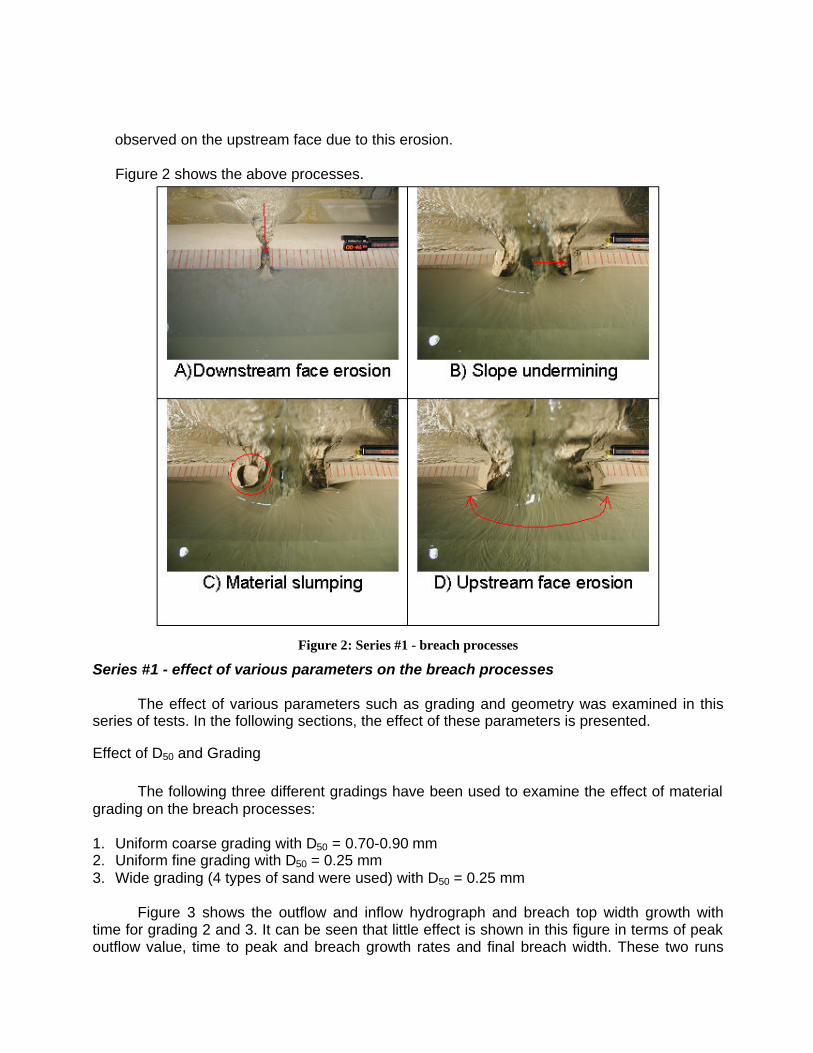
observed on the upstream face due to this erosion.
Figure 2 shows the above processes.
Figure 2: Series #1 - breach processes
Series #1 - effect of various parameters on the breach processes The effect of various parameters such as grading and geometry was examined in this
series of tests. In the following sections, the effect of these parameters is presented.
Effect of D50 and Grading The following three different gradings have been used to examine the effect of material
grading on the breach processes: 1. Uniform coarse grading with D50 = 0.70-0.90 mm 2. Uniform fine grading with D50 = 0.25 mm 3. Wide grading (4 types of sand were used) with D50 = 0.25 mm
Figure 3 shows the outflow and inflow hydrograph and breach top width growth with
time for grading 2 and 3. It can be seen that little effect is shown in this figure in terms of peak outflow value, time to peak and breach growth rates and final breach width. These two runs
show that the effect of grading is insignificant at this laboratory scale.
-0.1
0
0.1
0.2
0.3
0.4
0.5
0.6
0.7
0.8
0.9
2700 2800 2900 3000 3100 3200 3300 3400 3500
Time (sec)
Dis
char
ge
(m3 /s
)
-0.5
0
0.5
1
1.5
2
2.5
3
3.5
4
4.5
Wid
th (
m)
Outflow Wide Grading
Inflow Wide Grading
Outflow Uniform FineGrading
Inflow Uniform Fine Grading
Breach Top Width UniformFine Grading
Breach Top Width WideGrading
Figure 33: Grading variation results
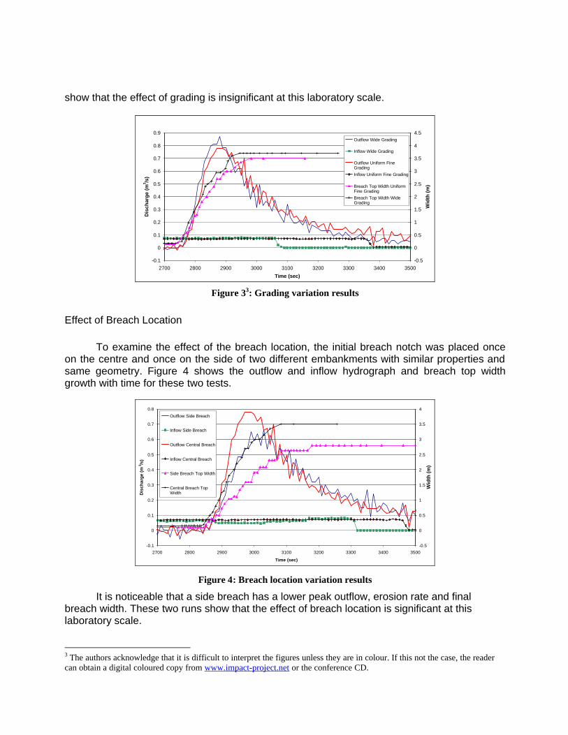
Effect of Breach Location To examine the effect of the breach location, the initial breach notch was placed once
on the centre and once on the side of two different embankments with similar properties and same geometry. Figure 4 shows the outflow and inflow hydrograph and breach top width growth with time for these two tests.
-0.1
0
0.1
0.2
0.3
0.4
0.5
0.6
0.7
0.8
2700 2800 2900 3000 3100 3200 3300 3400 3500
Time (sec)
Dis
char
ge
(m3 /s
)
-0.5
0
0.5
1
1.5
2
2.5
3
3.5
4
Wid
th (
m)
Outflow Side Breach
Inflow Side Breach
Outflow Central Breach
Inflow Central Breach
Side Breach Top Width
Central Breach TopWidth
Figure 4: Breach location variation results
It is noticeable that a side breach has a lower peak outflow, erosion rate and final breach width. These two runs show that the effect of breach location is significant at this laboratory scale.
3 The authors acknowledge that it is difficult to interpret the figures unless they are in colour. If this not the case, the reader can obtain a digital coloured copy from www.impact-project.net or the conference CD.
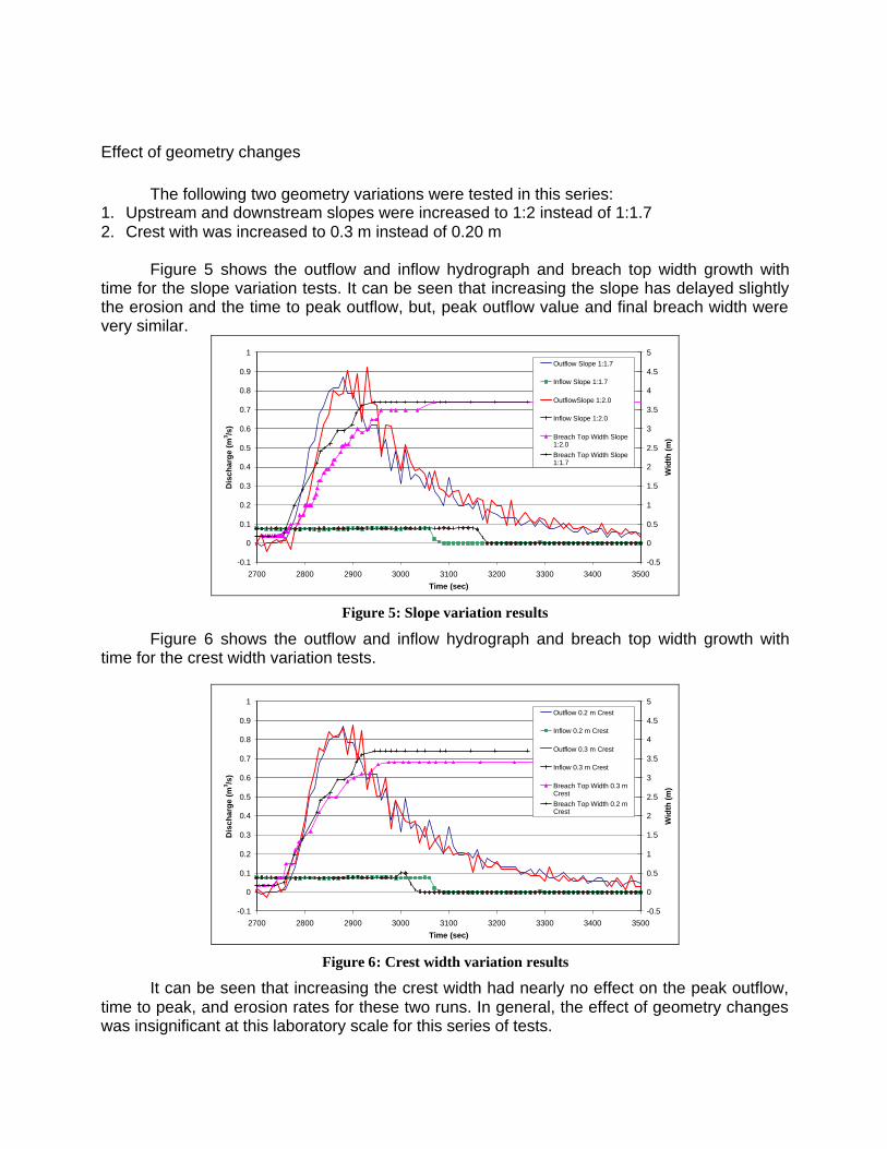
Effect of geometry changes The following two geometry variations were tested in this series:
1. Upstream and downstream slopes were increased to 1:2 instead of 1:1.7 2. Crest with was increased to 0.3 m instead of 0.20 m
Figure 5 shows the outflow and inflow hydrograph and breach top width growth with time for the slope variation tests. It can be seen that increasing the slope has delayed slightly the erosion and the time to peak outflow, but, peak outflow value and final breach width were very similar.
-0.1
0
0.1
0.2
0.3
0.4
0.5
0.6
0.7
0.8
0.9
1
2700 2800 2900 3000 3100 3200 3300 3400 3500
Time (sec)
Dis
char
ge
(m3 /s
)
-0.5
0
0.5
1
1.5
2
2.5
3
3.5
4
4.5
5
Wid
th (
m)
Outflow Slope 1:1.7
Inflow Slope 1:1.7
OutflowSlope 1:2.0
Inflow Slope 1:2.0
Breach Top Width Slope1:2.0
Breach Top Width Slope1:1.7
Figure 5: Slope variation results
Figure 6 shows the outflow and inflow hydrograph and breach top width growth with time for the crest width variation tests.
-0.1
0
0.1
0.2
0.3
0.4
0.5
0.6
0.7
0.8
0.9
1
2700 2800 2900 3000 3100 3200 3300 3400 3500
Time (sec)
Dis
char
ge
(m3 /s
)
-0.5
0
0.5
1
1.5
2
2.5
3
3.5
4
4.5
5
Wid
th (
m)
Outflow 0.2 m Crest
Inflow 0.2 m Crest
Outflow 0.3 m Crest
Inflow 0.3 m Crest
Breach Top Width 0.3 mCrest
Breach Top Width 0.2 mCrest
Figure 6: Crest width variation results
It can be seen that increasing the crest width had nearly no effect on the peak outflow, time to peak, and erosion rates for these two runs. In general, the effect of geometry changes was insignificant at this laboratory scale for this series of tests.
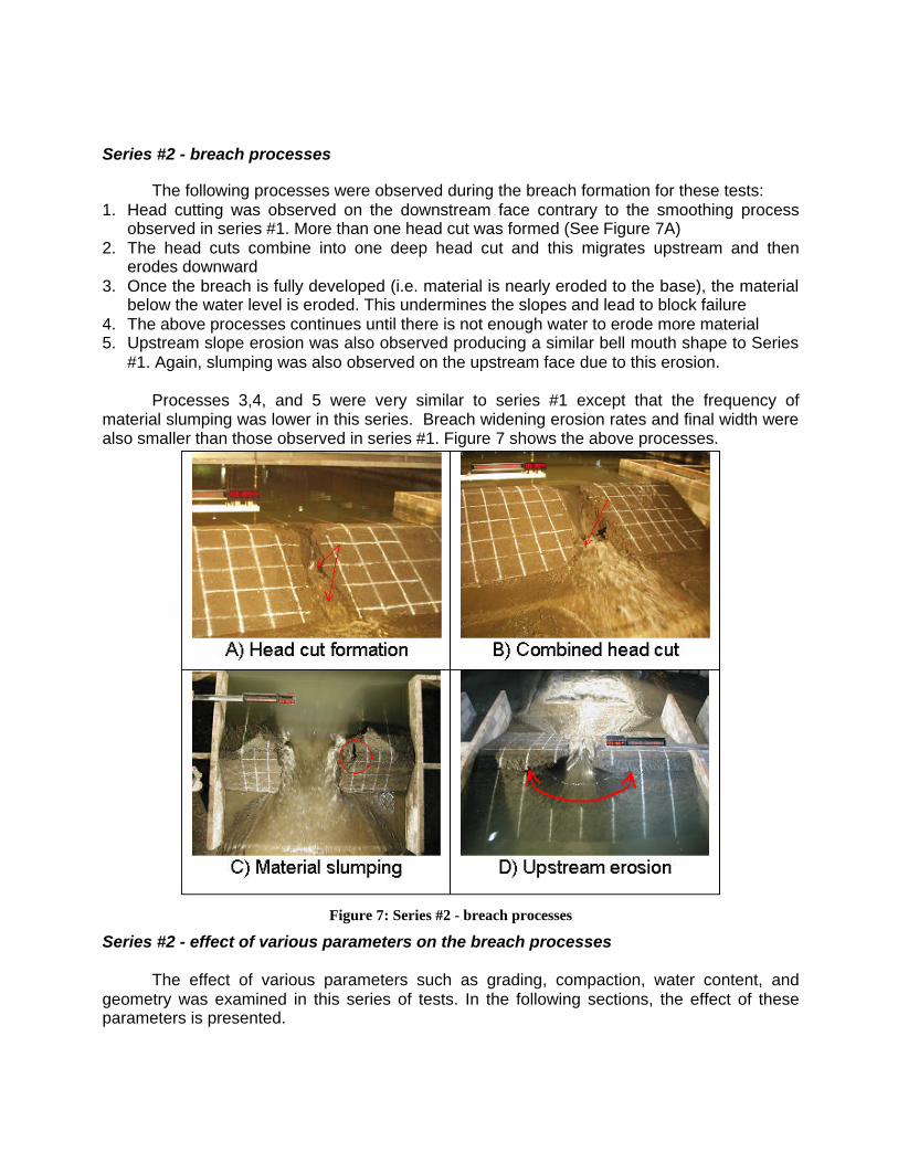
Series #2 - breach processes
The following processes were observed during the breach formation for these tests: 1. Head cutting was observed on the downstream face contrary to the smoothing process
observed in series #1. More than one head cut was formed (See Figure 7A) 2. The head cuts combine into one deep head cut and this migrates upstream and then
erodes downward 3. Once the breach is fully developed (i.e. material is nearly eroded to the base), the material
below the water level is eroded. This undermines the slopes and lead to block failure 4. The above processes continues until there is not enough water to erode more material 5. Upstream slope erosion was also observed producing a similar bell mouth shape to Series
#1. Again, slumping was also observed on the upstream face due to this erosion.
Processes 3,4, and 5 were very similar to series #1 except that the frequency of material slumping was lower in this series. Breach widening erosion rates and final width were also smaller than those observed in series #1. Figure 7 shows the above processes.
Figure 7: Series #2 - breach processes
Series #2 - effect of various parameters on the breach processes The effect of various parameters such as grading, compaction, water content, and
geometry was examined in this series of tests. In the following sections, the effect of these parameters is presented.
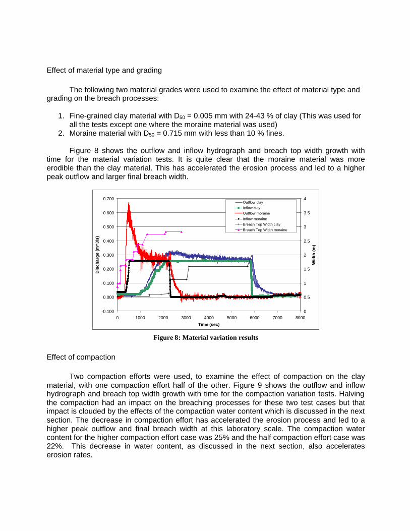
Effect of material type and grading The following two material grades were used to examine the effect of material type and
grading on the breach processes: 1. Fine-grained clay material with D50 = 0.005 mm with 24-43 % of clay (This was used for
all the tests except one where the moraine material was used) 2. Moraine material with D50 = 0.715 mm with less than 10 % fines.
Figure 8 shows the outflow and inflow hydrograph and breach top width growth with time for the material variation tests. It is quite clear that the moraine material was more erodible than the clay material. This has accelerated the erosion process and led to a higher peak outflow and larger final breach width.
-0.100
0.000
0.100
0.200
0.300
0.400
0.500
0.600
0.700
0 1000 2000 3000 4000 5000 6000 7000 8000
Time (sec)
Dis
char
ge
(m^3
/s)
0
0.5
1
1.5
2
2.5
3
3.5
4
Wid
th (
m)
Outflow clay
Inflow clay
Outflow moraine
Inflow moraine
Breach Top Width clay
Breach Top Width moraine
Figure 8: Material variation results
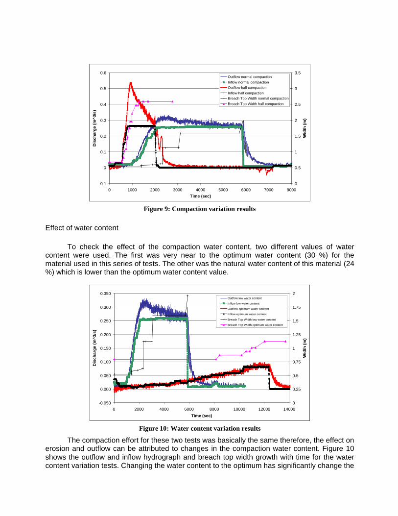
Effect of compaction Two compaction efforts were used, to examine the effect of compaction on the clay
material, with one compaction effort half of the other. Figure 9 shows the outflow and inflow hydrograph and breach top width growth with time for the compaction variation tests. Halving the compaction had an impact on the breaching processes for these two test cases but that impact is clouded by the effects of the compaction water content which is discussed in the next section. The decrease in compaction effort has accelerated the erosion process and led to a higher peak outflow and final breach width at this laboratory scale. The compaction water content for the higher compaction effort case was 25% and the half compaction effort case was 22%. This decrease in water content, as discussed in the next section, also accelerates erosion rates.
-0.1
0
0.1
0.2
0.3
0.4
0.5
0.6
0 1000 2000 3000 4000 5000 6000 7000 8000
Time (sec)
Dis
char
ge
(m^3
/s)
0
0.5
1
1.5
2
2.5
3
3.5
Wid
th (
m)
Outflow normal compaction
Inflow normal compaction
Outflow half compaction
Inflow half compaction
Breach Top Width normal compaction
Breach Top Width half compaction
Figure 9: Compaction variation results
Effect of water content To check the effect of the compaction water content, two different values of water
content were used. The first was very near to the optimum water content (30 %) for the material used in this series of tests. The other was the natural water content of this material (24 %) which is lower than the optimum water content value.
-0.050
0.000
0.050
0.100
0.150
0.200
0.250
0.300
0.350
0 2000 4000 6000 8000 10000 12000 14000
Time (sec)
Dis
char
ge
(m^3
/s)
0
0.25
0.5
0.75
1
1.25
1.5
1.75
2
Wid
th (
m)
Outflow low water content
Inflow low water content
Outflow optimum water content
Inflow optimum water content
Breach Top Width low water content
Breach Top Width optimum water content
Figure 10: Water content variation results
The compaction effort for these two tests was basically the same therefore, the effect on erosion and outflow can be attributed to changes in the compaction water content. Figure 10 shows the outflow and inflow hydrograph and breach top width growth with time for the water content variation tests. Changing the water content to the optimum has significantly change the
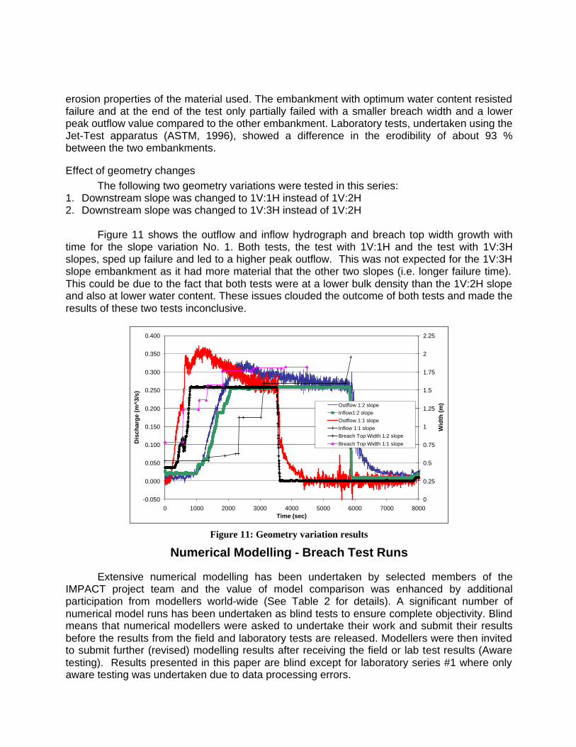
erosion properties of the material used. The embankment with optimum water content resisted failure and at the end of the test only partially failed with a smaller breach width and a lower peak outflow value compared to the other embankment. Laboratory tests, undertaken using the Jet-Test apparatus (ASTM, 1996), showed a difference in the erodibility of about 93 % between the two embankments.
Effect of geometry changes The following two geometry variations were tested in this series:
1. Downstream slope was changed to 1V:1H instead of 1V:2H 2. Downstream slope was changed to 1V:3H instead of 1V:2H
Figure 11 shows the outflow and inflow hydrograph and breach top width growth with time for the slope variation No. 1. Both tests, the test with 1V:1H and the test with 1V:3H slopes, sped up failure and led to a higher peak outflow. This was not expected for the 1V:3H slope embankment as it had more material that the other two slopes (i.e. longer failure time). This could be due to the fact that both tests were at a lower bulk density than the 1V:2H slope and also at lower water content. These issues clouded the outcome of both tests and made the results of these two tests inconclusive.
-0.050
0.000
0.050
0.100
0.150
0.200
0.250
0.300
0.350
0.400
0 1000 2000 3000 4000 5000 6000 7000 8000Time (sec)
Dis
char
ge
(m^3
/s)
0
0.25
0.5
0.75
1
1.25
1.5
1.75
2
2.25
Wid
th (
m)Outflow 1:2 slope
Inflow1:2 slope
Outflow 1:1 slope
Inflow 1:1 slope
Breach Top Width 1:2 slope
Breach Top Width 1:1 slope
Figure 11: Geometry variation results
Numerical Modelling - Breach Test Runs
Extensive numerical modelling has been undertaken by selected members of the IMPACT project team and the value of model comparison was enhanced by additional participation from modellers world-wide (See Table 2 for details). A significant number of numerical model runs has been undertaken as blind tests to ensure complete objectivity. Blind means that numerical modellers were asked to undertake their work and submit their results before the results from the field and laboratory tests are released. Modellers were then invited to submit further (revised) modelling results after receiving the field or lab test results (Aware testing). Results presented in this paper are blind except for laboratory series #1 where only aware testing was undertaken due to data processing errors.
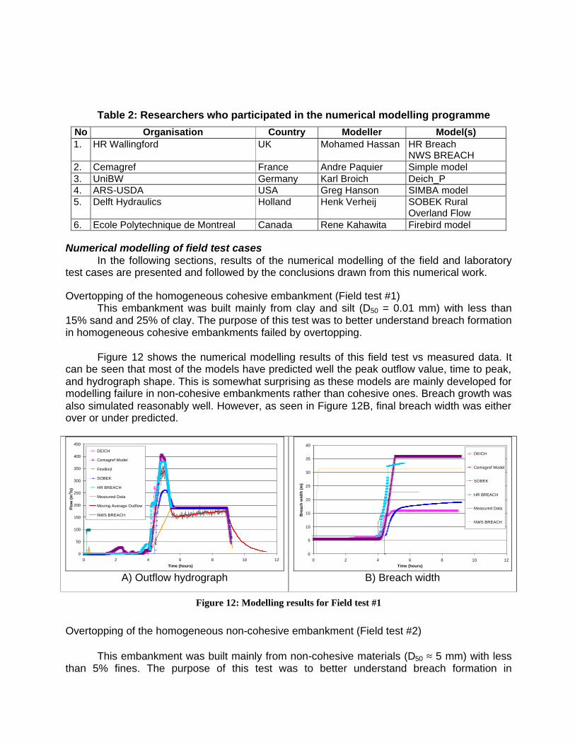
Table 2: Researchers who participated in the numerical modelling programme
No Organisation Country Modeller Model(s) 1. HR Wallingford UK Mohamed Hassan HR Breach
NWS BREACH 2. Cemagref France Andre Paquier Simple model 3. UniBW Germany Karl Broich Deich_P 4. ARS-USDA USA Greg Hanson SIMBA model 5. Delft Hydraulics Holland Henk Verheij SOBEK Rural
Overland Flow 6. Ecole Polytechnique de Montreal Canada Rene Kahawita Firebird model
Numerical modelling of field test cases
In the following sections, results of the numerical modelling of the field and laboratory test cases are presented and followed by the conclusions drawn from this numerical work. Overtopping of the homogeneous cohesive embankment (Field test #1)
This embankment was built mainly from clay and silt (D50 = 0.01 mm) with less than 15% sand and 25% of clay. The purpose of this test was to better understand breach formation in homogeneous cohesive embankments failed by overtopping.
Figure 12 shows the numerical modelling results of this field test vs measured data. It
can be seen that most of the models have predicted well the peak outflow value, time to peak, and hydrograph shape. This is somewhat surprising as these models are mainly developed for modelling failure in non-cohesive embankments rather than cohesive ones. Breach growth was also simulated reasonably well. However, as seen in Figure 12B, final breach width was either over or under predicted.
0
50
100
150
200
250
300
350
400
450
0 2 4 6 8 10 12
Time (hours)
Flo
w (
m3 /s
)
DEICH
Cemagref Model
FireBird
SOBEK
HR BREACH
Measured Data
Moving Average Outflow
NWS BREACH
A) Outflow hydrograph
0
5
10
15
20
25
30
35
40
0 2 4 6 8 10 12Time (hours)
Bre
ach
wid
th (
m)
DEICH
Cemagref Model
SOBEK
HR BREACH
Measured Data
NWS BREACH
B) Breach width
Figure 12: Modelling results for Field test #1
Overtopping of the homogeneous non-cohesive embankment (Field test #2)
This embankment was built mainly from non-cohesive materials (D50 ≈ 5 mm) with less
than 5% fines. The purpose of this test was to better understand breach formation in
homogeneous non-cohesive embankments failed by overtopping.
0
20
40
60
80
100
120
140
0 1000 2000 3000 4000 5000 6000 7000 8000 9000 10000
Time (s)
Ou
tflo
w (
m3/
s)
DEICH
CemagrefModelSOBEK
MeasuredDataHR BREACH
NWSBREACH
A) Outflow hydrograph
0
2
4
6
8
10
12
14
16
0 1000 2000 3000 4000 5000 6000 7000 8000 9000 10000
Time (s)
Ou
tflo
w (
m3/
s)
DEICH Cemagref Model SOBEK HR BREACH NWS BREACH
B) Breach width
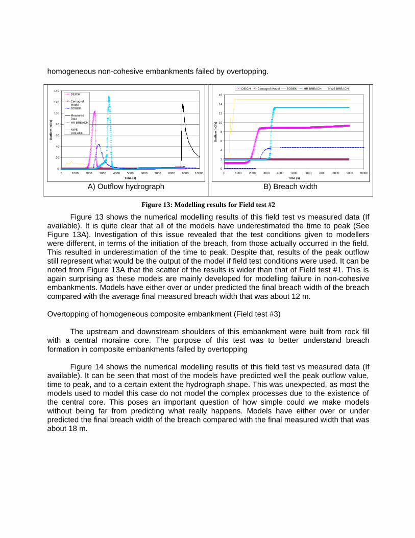
Figure 13: Modelling results for Field test #2
Figure 13 shows the numerical modelling results of this field test vs measured data (If available). It is quite clear that all of the models have underestimated the time to peak (See Figure 13A). Investigation of this issue revealed that the test conditions given to modellers were different, in terms of the initiation of the breach, from those actually occurred in the field. This resulted in underestimation of the time to peak. Despite that, results of the peak outflow still represent what would be the output of the model if field test conditions were used. It can be noted from Figure 13A that the scatter of the results is wider than that of Field test #1. This is again surprising as these models are mainly developed for modelling failure in non-cohesive embankments. Models have either over or under predicted the final breach width of the breach compared with the average final measured breach width that was about 12 m. Overtopping of homogeneous composite embankment (Field test #3)
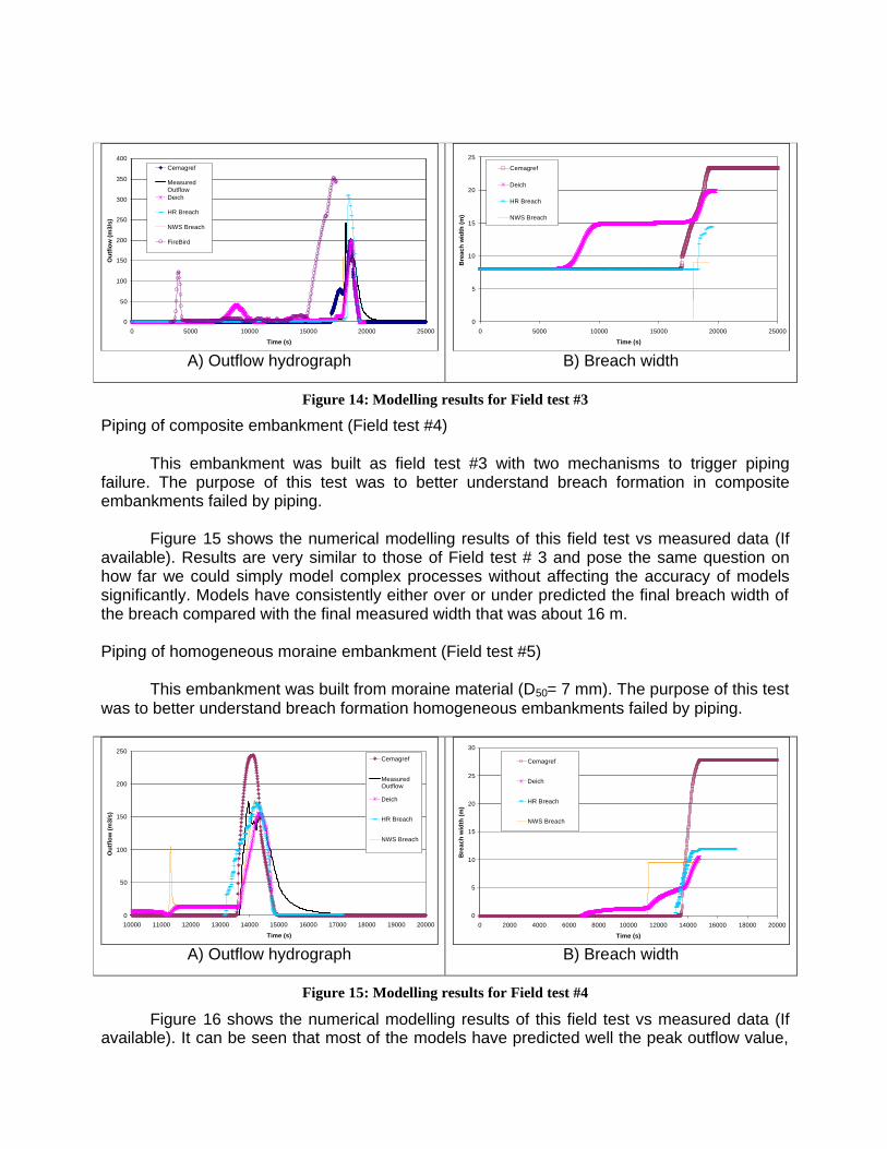
The upstream and downstream shoulders of this embankment were built from rock fill with a central moraine core. The purpose of this test was to better understand breach formation in composite embankments failed by overtopping
Figure 14 shows the numerical modelling results of this field test vs measured data (If available). It can be seen that most of the models have predicted well the peak outflow value, time to peak, and to a certain extent the hydrograph shape. This was unexpected, as most the models used to model this case do not model the complex processes due to the existence of the central core. This poses an important question of how simple could we make models without being far from predicting what really happens. Models have either over or under predicted the final breach width of the breach compared with the final measured width that was about 18 m.
0
50
100
150
200
250
300
350
400
0 5000 10000 15000 20000 25000
Time (s)
Ou
tflo
w (
m3/
s)
Cemagref
MeasuredOutflowDeich
HR Breach
NWS Breach
FireBird
A) Outflow hydrograph
0
5
10
15
20
25
0 5000 10000 15000 20000 25000
Time (s)
Bre
ach
wid
th (
m)
Cemagref
Deich
HR Breach
NWS Breach
B) Breach width
Figure 14: Modelling results for Field test #3
Piping of composite embankment (Field test #4)
This embankment was built as field test #3 with two mechanisms to trigger piping failure. The purpose of this test was to better understand breach formation in composite embankments failed by piping.
Figure 15 shows the numerical modelling results of this field test vs measured data (If available). Results are very similar to those of Field test # 3 and pose the same question on how far we could simply model complex processes without affecting the accuracy of models significantly. Models have consistently either over or under predicted the final breach width of the breach compared with the final measured width that was about 16 m.
Piping of homogeneous moraine embankment (Field test #5)
This embankment was built from moraine material (D50= 7 mm). The purpose of this test was to better understand breach formation homogeneous embankments failed by piping.
0
50
100
150
200
250
10000 11000 12000 13000 14000 15000 16000 17000 18000 19000 20000
Time (s)
Ou
tflo
w (
m3/
s)
Cemagref
MeasuredOutflow
Deich
HR Breach
NWS Breach
A) Outflow hydrograph
0
5
10
15
20
25
30
0 2000 4000 6000 8000 10000 12000 14000 16000 18000 20000
Time (s)
Bre
ach
wid
th (
m)
Cemagref
Deich
HR Breach
NWS Breach
B) Breach width
Figure 15: Modelling results for Field test #4
Figure 16 shows the numerical modelling results of this field test vs measured data (If available). It can be seen that most of the models have predicted well the peak outflow value,
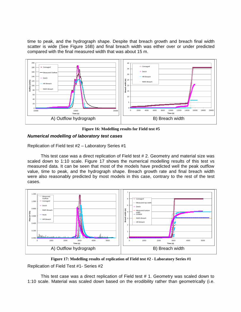
time to peak, and the hydrograph shape. Despite that breach growth and breach final width scatter is wide (See Figure 16B) and final breach width was either over or under predicted compared with the final measured width that was about 15 m.
0
20
40
60
80
100
120
140
160
180
200
10000 15000 20000
Time (s)
Ou
tflo
w (
m3/
s)
Cemagref
Measured Outflow
Deich
HR Breach
NWS Breach
A) Outflow hydrograph
0
5
10
15
20
25
30
35
40
0 2000 4000 6000 8000 10000 12000 14000 16000 18000 20000
Time (s)
Bre
ach
wid
th (
m)
Cemagref
Deich
HR Breach
NWS Breach
B) Breach width
Figure 16: Modelling results for Field test #5
Numerical modelling of laboratory test cases Replication of Field test #2 – Laboratory Series #1
This test case was a direct replication of Field test # 2. Geometry and material size was
scaled down to 1:10 scale. Figure 17 shows the numerical modelling results of this test vs measured data. It can be seen that most of the models have predicted well the peak outflow value, time to peak, and the hydrograph shape. Breach growth rate and final breach width were also reasonably predicted by most models in this case, contrary to the rest of the test cases.
0.000
0.200
0.400
0.600
0.800
1.000
1.200
0 1000 2000 3000 4000 5000
Time (s)
Flo
w (
m^3
/s)
MeasuredOutflow
Cemagref
Deich
NWS Breach
Henk
HR Breach
A) Outflow hydrograph
0
1
2
3
4
5
6
7
0 1000 2000 3000 4000 5000
Time (s)
Bre
ach
wid
th (
m)
Cemagref
Measured top width
Deich
Measured bottomwidthSOBEK
NWS Breach
HR Breach
B) Breach width
Figure 17: Modelling results of replication of Field test #2 - Laboratory Series #1
Replication of Field Test #1- Series #2
This test case was a direct replication of Field test # 1. Geometry was scaled down to 1:10 scale. Material was scaled down based on the erodibility rather than geometrically (i.e.
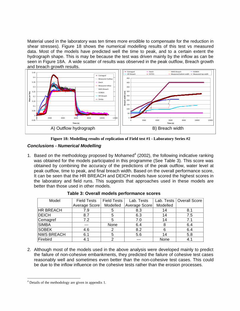
Material used in the laboratory was ten times more erodible to compensate for the reduction in shear stresses). Figure 18 shows the numerical modelling results of this test vs measured data. Most of the models have predicted well the time to peak, and to a certain extent the hydrograph shape. This is may be because the test was driven mainly by the inflow as can be seen in Figure 18A. A wide scatter of results was observed in the peak outflow, Breach growth and breach growth results.
-0.05
0
0.05
0.1
0.15
0.2
0.25
0.3
0.35
0.4
0.45
0 2000 4000 6000 8000 10000 12000
Time (s)
Flo
w (
m^3
/s)
Cemagref
Measured Outflow
Deich
Measured Inflow
NWS Breach
SOBEK
HR Breach
Simba
A) Outflow hydrograph
0
50
100
150
200
250
300
350
400
450
0 2000 4000 6000 8000 10000 12000
Time (s)B
reac
h w
idth
(cm
)
Cemagref Deich NWS Breach SOBEKHR Breach SITES Measured bottom width Measured top width
B) Breach width
Figure 18: Modelling results of replication of Field test #1 - Laboratory Series #2
Conclusions - Numerical Modelling 1. Based on the methodology proposed by Mohamed4 (2002), the following indicative ranking
was obtained for the models participated in this programme (See Table 3). This score was obtained by combining the accuracy of the predictions of the peak outflow, water level at peak outflow, time to peak, and final breach width. Based on the overall performance score, It can be seen that the HR BREACH and DEICH models have scored the highest scores in the laboratory and field runs. This suggests that approaches used in these models are better than those used in other models.
Table 3: Overall models performance scores
Model Field Tests Average Score
Field Tests Modelled
Lab. Tests Average Score
Lab. Tests Modelled
Overall Score
HR BREACH 7.9 5 8.3 14 8.1 DEICH 8.7 5 6.3 14 7.5 Cemagref 7.2 5 7.0 14 7.1 SIMBA --- None 6.4 8 6.4 SOBEK 4.6 2 8.2 6 6.4 NWS BREACH 6.1 5 5.6 14 5.8 Firebird 4.1 2 --- None 4.1
2. Although most of the models used in the above analysis were developed mainly to predict
the failure of non-cohesive embankments, they predicted the failure of cohesive test cases reasonably well and sometimes even better than the non-cohesive test cases. This could be due to the inflow influence on the cohesive tests rather than the erosion processes.
4 Details of the methodology are given in appendix 1.

3. All models, for field and laboratory tests, have either overestimated or underestimated the breach width. This might be because most of these models were not calibrated or verified with breach growth data or this is the effect of using sediment transport equations not suitable or valid for breach test conditions.
4. The test conditions of Field Test # 2 delayed the failure of the dam by about 4 times the
time predicted by most of the models. This highlights the importance of including site specific properties when modelling the failure of embankments.
References
1. ASTM (1996). Designation: D5852-95 Standard Test Method for Erodibility Determination
of Soil in the Field or in the Laboratory by the Jet Index Method. Annual Book of ASTM (American Society for Testing and Materials) Standards, Section 4 Construction, Volume 04.09 Soil and Rock.
2. Mohamed, M. (2002). Embankment Breach Formation and Modelling Methods. PhD. Thesis, The Open University.
Appendix 1: Numerical modelling scoring system Model performance is judged by a category and score. Based on the difference in percentage between the measured and predicted values, the following categories are suggested: 1. Very Good Performance. 2. Good Performance 3. Reasonable Performance 4. Satisfactory Performance 5. Unsatisfactory Performance 6. Inadequate Performance
These categories overlap as shown in Figure 20. The score is a number represents the model performance and it is computed based on these categories. If the difference between the measured and the predicted data is more than ±50 %, the model performance is considered unacceptable and the score is assumed to be zero. Parameters can also be weighted according to their importance. The overall performance of the models can be calculated according to the following formula (Other terms can also be added to the above formula to take into consideration other parameters such as breach dimensions, growth rate, etc..):
......
......**
++
++=
sTsQ
sTTsQQ
s CC
CSCST (1)
where: Ts : Overall score of the model performance. SQ : Outflow of the model score. ST : Time to peak score CsQ : Outflow weighting factor. CsT : Time to peak weighting factor.
Acknowledgements The Authors wish to thank IMPACT project partners particularly André Paquier, Karl Broich, and Kjetil Vaskinn for their valuable help and the European Commission for funding this project. The Authors are also grateful for the Association of State Dam Safety Officials and the
Figure 19: Model performance criteria
0
25
50
75
100
± 10% ± 20% ± 30% ± 40%
V. Good Good
Satisfactory Unsatisfactory
Reasonable
Key:
± 50%
Inadequate
10 9 8 7 6 5Score
% Diff.
% S
core

Egyptian Ministry of Water Resources and Irrigation for their valuable support.
Top Related