


Languages
Pages
Legal

Bistability, Spatial Interaction, andthe Distribution of Tropical Forests
and Savannas
Arie Staal,1* Stefan C. Dekker,2 Chi Xu,3 and Egbert H. van Nes1
1Aquatic Ecology and Water Quality Management Group, Department of Environmental Sciences, Wageningen University, P.O.Box 47, 6700 AA Wageningen, The Netherlands; 2Department of Environmental Sciences, Copernicus Institute for Sustainable
Development, Utrecht University, P.O. Box 80115, 3508 TC Utrecht, The Netherlands; 3School of Life Sciences, Nanjing University,
163 Xianlin Road, Nanjing 210023, China
ABSTRACT
Recent work has indicated that tropical forest and
savanna can be alternative stable states under a
range of climatic conditions. However, dynamical
systems theory suggests that in case of strong spa-
tial interactions between patches of forest and sa-
vanna, a boundary between both states is only
possible at conditions in which forest and savanna
are equally stable, called the ‘Maxwell point.’ Fre-
quency distributions of MODIS tree-cover data at
250 m resolution were used to estimate such
Maxwell points with respect to the amount and
seasonality of rainfall in both South America and
Africa. We tested on a 0.5� scale whether there is a
larger probability of local coexistence of forests and
savannas near the estimated Maxwell points.
Maxwell points for South America and Africa were
estimated at 1760 and 1580 mm mean annual
precipitation and at Markham’s Seasonality Index
values of 50 and 24 %. Although the probability of
local coexistence was indeed highest around these
Maxwell points, local coexistence was not limited
to the Maxwell points. We conclude that critical
transitions between forest and savanna may occur
when climatic changes exceed a critical value.
However, we also conclude that spatial interactions
between patches of forest and savanna may reduce
the hysteresis that can be observed in isolated
patches, causing more predictable forest-savanna
boundaries than continental-scale analyses of tree
cover indicate. This effect could be less pronounced
in Africa than in South America, where the forest-
savanna boundary is substantially affected by
rainfall seasonality.
Key words: catastrophe theory; climate change;
critical transition; ecotone; wildfire; Maxwell point;
reaction–diffusion system; regime shift; remote
sensing; tipping point.
INTRODUCTION
The idea that the distribution of Earth’s biomes is
governed by ‘climate envelopes’ has a long history
(Von Humboldt and Bonpland 1807; Schimper
1903). According to this view, climate has a
deterministic effect on vegetation types, implying
that the locations of stable biome boundaries are
predictable. Correspondingly, the distributions of
the biomes on Earth, such as tropical forests and
savannas, are expected to shift gradually with
Received 27 May 2015; accepted 24 March 2016;
published online 30 June 2016
Electronic supplementary material: The online version of this article
(doi:10.1007/s10021-016-0011-1) contains supplementary material,
which is available to authorized users.
Author contributions A.S., S.C.D., and E.H.v.N. conceived and de-
signed the study. A.S. performed the research. A.S. and C.X. analyzed
data. A.S. wrote the paper with contributions from all authors.
*Corresponding author; e-mail: [email protected]
Ecosystems (2016) 19: 1080–1091DOI: 10.1007/s10021-016-0011-1
� 2016 The Author(s). This article is published with open access at Springerlink.com
1080
gradual climate change. In recent years, however,
evidence has been growing that the effect of cli-
mate on tropical forests and savannas is non-linear
(Reyer and others 2015). Notably, studies based on
satellite data of tree cover showed that under a
range of mean annual precipitation (MAP) high
frequencies of both savanna (�20 %) and forest
tree-cover levels (�80 %) can be found, whereas
intermediate values are rare (Hirota and others
2011; Staver and others 2011b). This bimodality of
tree cover in both satellite data and field data under
given environmental conditions indicates that for-
est and savanna may represent separate basins of
attraction, which is simply referred to as alternative
stable states (Scheffer and Carpenter 2003; Hirota
and others 2011). An important mechanism that
could explain such bistability is a feedback between
grass and fire (Staver and others 2011b; Murphy
and Bowman 2012; Dantas and others 2016). In
savannas, grasses act as fuel for fires (Bond 2008).
Savanna trees are adapted to fires by allocating
many resources to developing thick barks (Keeley
and others 2011). However, this resource allocation
implies investing less resources in leaf area than
forest tree species do (Silva and others 2013). Be-
cause the open canopy in savannas allows fires to
occur and the closed canopy in forests suppresses
fire, both states are self-stabilizing (Murphy and
Bowman 2012). Drought, however, may destabi-
lize a forest by allowing it to burn. Burned forests
can be invaded by grasses that facilitate recurrent
fires (Brando and others 2014), which may trigger
a transition to savanna. The reverse transition oc-
curs if a fire-free interval exceeds a threshold,
determined by available resources, above which
forest-tree species can form a closed canopy (Hoff-
mann and others 2012). The theory of alternative
stable states (Scheffer and others 2001) predicts
that bistable systems can undergo a transition from
one state to the other if environmental conditions
(such as MAP) reach a so-called ‘tipping point.’
After a transition has occurred, the system may not
easily recover to the original state even if the
change in conditions is reversed, a phenomenon
called hysteresis. Hysteresis implies that there is a
range of conditions at which either state can be
present and large stochastic disturbances could
cause transitions between the states (the bistability
range). Therefore, in a bistable forest-savanna sys-
tem, boundaries are difficult to predict based on
external conditions (Moncrieff and others 2016).
Hence, bistability of forest and savanna on the one
hand, and the climatic-deterministic explanation of
forest-savanna distributions on the other, seem to
represent two fundamentally incompatible views.
Experiments to test hysteresis are challenging,
especially on landscape-scale systems such as for-
ests and savannas (Bowman and others 2015). So
far, experiments on alternative stable states are
either conducted in laboratory microcosms (for
example, Dai and others 2013) or on isolated
ecosystems (Carpenter and others 2011). More-
over, theoretical studies of alternative stable states
often use simple models that assume well-mixed
systems without explicit consideration of spatial
components (Scheffer 2009). However, the
behavior of such models can change considerably
when local spatial interactions are taken into ac-
count (Wilson and others 1996; Bel and others
2012; Van de Leemput and others 2015; Villa
Martın and others 2015). Spatial interactions are
usually modeled in reaction–diffusion equations
where the relevant state variables (such as bio-
mass) have local dynamics (‘reaction’) and ex-
change between neighboring patches (‘diffusion’).
In the case of forest and savanna, this biomass ex-
change between neighboring cells would capture,
in a simple manner, mechanisms by which forest
patches increase tree cover in neighboring savanna
patches (for example, by means of seed dispersal)
and by which savanna patches decrease tree cover
in neighboring forest patches (for example, by
means of fire spread). If patches of forest and sa-
vanna spatially interact in such a way, then
boundaries between alternative stable states may
become unstable, meaning that the two states
cannot coexist on a local scale. This impossibility of
local coexistence of alternative stable states is a
generic result in partial differential equations,
regardless of the specific mechanisms that cause
bistability (Murray 2002; Van de Leemput and
others 2015). However, whether destabilization of
local coexistence occurs depends on how strong
these mechanisms are relative to spatial interac-
tions. With an increase in spatial interaction
strength, the range of environmental conditions at
which local coexistence of alternative states is
possible becomes smaller (Van de Leemput and
others 2015). In cases with very strong spatial
interactions, it becomes inevitable that at given
conditions the most stable alternative state will
eventually dominate. This is because even if the
landscape is occupied by the least stable state, a
local invasion by the most stable state is sufficient
to trigger a domino effect of a spatial transition to
that state (Pomeau 1986; Wilson and others 1996).
This implies that in a gradient of environmental
conditions, the boundary between the alternative
stable states is highly predictable as it occurs at the
conditions where both states are equally
Bistability, Spatial Interaction, and the Distribution of Tropical Forests and Savannas 1081

stable (Wilson and others 1996; Van de Leemput
and others 2015). It also implies that there is no
hysteresis in response to changing environmental
conditions as transitions between alternative states
always occur when the conditions of equal stability
are crossed (Figure 1). Environmental conditions of
equal stability are referred to as the Maxwell point
(after Maxwell 1875). In cases where spatial
interactions are so strong that hysteresis is elimi-
nated, the system is said to follow the ‘Maxwell
convention.’ With increasing spatial interaction
strength, hysteresis becomes more narrow. If spa-
tial interactions are negligible, the system is said to
follow the ‘delay convention’ (Gilmore 1981; Fort
2013). In such cases the patches can be in either
state independently of the state of neighboring cells
and the patches can be in either state over a range
of conditions. Moreover, hysteresis will make the
conditions at which boundaries between alterna-
tive stable states are found unpredictable.
Which of the two conventions applies to forest-
savanna dynamics is unclear. Forest-savanna
dynamics can be characterized as patch dynamics
(Goetze and others 2006; Dantas and others 2013)
acting on the scale of several hundreds of meters
(Favier and others 2012). When patches do not
interact, the delay convention would apply, which
means that we may expect a roughly equal distri-
bution of local coexistence of patches of forest and
savanna along a range of environmental condi-
tions, corresponding to the bistability range (see
Appendix S1 for a modeling example). If, however,
there are significant interactions between patches,
the range where the two states can coexist locally
would become smaller than the bistability range for
isolated patches. The narrowing of the range of
conditions with local coexistence depends on the
spatial interaction strength, with the ultimate pos-
sibility that there will be only one point where a
stable boundary between both states is possible. In
this ultimate case the Maxwell convention would
apply, which means that we would find a distinctly
peaked distribution of local coexistence of patches
of forest and savanna around the Maxwell point.
In this study, we aimed to identify climatic
Maxwell points and test whether forests and
savannas in South America and Africa tend to
coexist at these conditions. If they tend to coexist
around a Maxwell point, then this would indicate
that shifts between forests and savannas in both
directions can be expected to occur when climatic
changes cross a Maxwell point, implying the ab-
sence of hysteresis. If forests and savannas tend to
coexist roughly equally throughout the bistability
range, then this would be consistent with the
classical tipping point model (the delay convention
Fig. 1. The theoretical effect of spatial interactions on critical transitions in a bistable system. a Without spatial interac-
tions between patches in an ecosystem, the patches undergo critical transitions between stable states (indicated by solid
lines; unstable equilibria are indicated with the dashed line) when conditions cross tipping points (vertical arrows). Thus, the
system displays hysteresis and therefore follows the ‘delay convention.’ b An increase in spatial interactions narrows the
range of conditions at which patches can be in alternative stable states. At other conditions the least stable state (indicated
by dotted lines) is not resilient against perturbations. Although the patches undergo critical transitions at different envi-
ronmental conditions than without spatial interactions between them, the system still displays hysteresis. c With strong
spatial interactions between patches, the least stable state is not resilient against perturbations: the invasion of at least one
patch of the most stable state results in dominance of that state in the landscape. Transitions in both directions occur at the
Maxwell point (double arrow). Thus, the system does not display hysteresis and therefore follows the ‘Maxwell conven-
tion.’ For this example, we used the model from Noy-Meir (1975), but the qualitative result is independent of the
bistable model used. Note that our simplified illustration ignores the effects of stochasticity, which allows for back-and-
forth transitions to occur in between the tipping points
1082 A. Staal and others
as in, for example, Van Nes and others 2014; Staal
and others 2015). In that case, shifts from forests to
savannas and vice versa can be expected at differ-
ent climatic conditions, implying hysteresis even in
spatially interacting landscapes. Because our study
differentiates between these two extremes, it im-
proves our understanding of the effect of climate
on forest-savanna boundaries and the catastrophic
behavior of forest-savanna shifts in response to
climate change.
METHODS
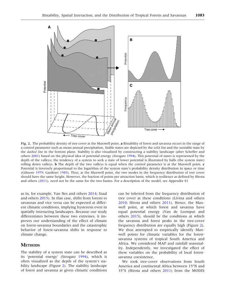
The stability of a system state can be described as
its ‘potential energy’ (Strogatz 1994), which is
often visualized as the depth of the system’s sta-
bility landscape (Figure 2). The stability landscape
of forest and savanna at given climatic conditions
can be inferred from the frequency distribution of
tree cover at these conditions (Livina and others
2010; Hirota and others 2011). Hence, the Max-
well point, at which forest and savanna have
equal potential energy (Van de Leemput and
others 2015), should be the conditions at which
the savanna and forest peaks in the tree-cover
frequency distribution are equally high (Figure 2).
We thus attempted to empirically identify Max-
well points for climatic variables for the forest-
savanna systems of tropical South America and
Africa. We considered MAP and rainfall seasonal-
ity. Independently, we investigated the effect of
these variables on the probability of local forest-
savanna coexistence.
We took tree-cover observations from South
America and continental Africa between 15�N and
35�S (Hirota and others 2011) from the MODIS
Fig. 2. The probability density of tree cover at the Maxwell point. a Bistability of forest and savanna occurs in the range of
a control parameter such as mean annual precipitation. Stable states are depicted by the solid line and the unstable state by
the dashed line in the bottom plane. Stability is also visualized by constructing a stability landscape (after Scheffer and
others 2001) based on the physical idea of potential energy (Strogatz 1994). This potential of states is represented by the
depth of the valleys; the tendency of a system to seek a state of lower potential is illustrated by balls (the system state)
rolling down valleys. b The depth of the two valleys is equal when the control parameter is at the Maxwell point. c
Potential is inversely proportional to the logarithm of the system state’s probability density distribution in space or time
(Gilmore 1979; Gardiner 1985). Thus, at the Maxwell point, the two modes in the frequency distribution of tree cover
should have the same height. However, the fraction of points per attraction basin, which is resilience as defined by Hirota
and others (2011), need not be the same for the two basins. For a description of the model, see Appendix S1
Bistability, Spatial Interaction, and the Distribution of Tropical Forests and Savannas 1083

Vegetation Continuous Field (VCF) Collection 5
dataset from 2009 at 250 m resolution (DiMiceli
and others 2011). We excluded human-used areas,
open water, and bare ground using the 2009 ESA
Globcover dataset (values 11–30 and ‡190) at
300 m resolution. However, this is an imperfect
exclusion of all human influence such as defor-
estation. We also excluded mountain regions
(‡1500 m elevation) using the Shuttle Radar
Topography Mission (SRTM) elevation data at
1 km resolution assembled by Hijmans and others
(2005). The resulting continental datasets consisted
each of more than 100 million observations. Pre-
cipitation data were taken from the Climate Re-
search Unit monthly dataset at 0.5� resolution
(Mitchell and Jones 2005). Seasonality of rainfall
was measured as Markham’s Seasonality Index
(MSI; Markham 1970):
MSI¼100
ffiffiffiffiffiffiffiffiffiffiffiffiffiffiffiffiffiffiffiffiffiffiffiffiffiffiffiffiffiffiffiffiffiffiffiffiffiffiffiffiffiffiffiffiffiffiffiffiffiffiffiffiffiffiffiffiffiffiffiffiffiffiffiffiffiffiffiffiffiffiffiffiffiffiffiffiffiffiffiffiffiffiffiffi
P
mPm sin m2p12
� �2h i
þP
mPm cos m2p12
� �2h i
r
P
mPm
MSI considers each monthly precipitation Pm value
to be a vector, where its direction is determined by
the time of year (in month number m) and its
length by the amount of rainfall. For each year,
monthly vectors are summed; the summed vector
is standardized by dividing by total rainfall over
the year. This generates an index that is inde-
pendent of MAP and ranges from 0 to 100 %,
where 0 implies an equal distribution of rainfall
over the months and 100 % implies that all rain-
fall occurs in a single month. Climatic variables
were calculated for the period 1961–2002. All
variables were resampled to a consistent spatial
resolution of 250 m.
For each continent, we investigated whether the
250 m tree-cover data indicate bistability of forest
and savanna within ranges of MAP (500–
2500 mm) and MSI (10–70 %). We inferred the
climatic ranges of bistability by analyzing the tree-
cover probability densities using potential analysis
(Livina and others 2010), which can be used to
construct stability landscapes (Figure 2). We ap-
plied this potential analysis to 1 & of the tree-cover
data points from each continent (Hirota and others
2011). We smoothed the densities of tree cover
with the MATLAB kernel smoothing function
ksdensity (with a bandwidth according to Silver-
man’s rule of thumb; Silverman 1986). We inferred
stable and unstable states of tree cover (minima
and maxima in the potentials) for moving windows
of the climatic variables (20 mm increments for
MAP and 1 % increments for MSI), where we ap-
plied Gaussian weights to the climatic variables
(standard deviation was 5 % of the entire range of
the climatic variable) (Hirota and others 2011). As
the MODIS VCF product used here is not without
bias (Hanan and others 2014, 2015), it precludes
detailed interpretations for specific tree-cover val-
ues. However, it has recently been validated that
observed forest-savanna bimodalities are no artifact
of the dataset (Staver and Hansen 2015), implying
that the bias is smaller than the signal. The ob-
served bimodalities have also been shown to be
consistent with independent Landsat data (Xu and
others 2015), providing sufficient support for the
use of the dataset for our purpose.
To estimate Maxwell points of forest and sa-
vanna, we randomly took from each continent a
sample of 1000 tree-cover data points for classes of
MAP (500–2500 mm; bin size 100 mm with
20 mm increments) and MSI (10–70 %; bin size
6 % with 1 % increments). We determined for
each sample whether the distribution was bimodal
by fitting both a uni- and bimodal distribution
using latent class analysis with the MATLAB
function gmdistribution. We adopted a conserva-
tive approach in determining whether the distri-
bution was bimodal by considering three criteria:
the bimodal distribution should have both (1) a
lower Akaike information criterion and (2) a lower
Bayesian information criterion than the unimodal
distribution, and (3) there should be a significant
(a = 0.05) deviation from a unimodal distribution
according to Hartigan’s dip test (Hartigan and
Hartigan 1985). Furthermore, because we were
interested in forest-savanna bimodality, we only
considered bimodal distributions of which the
modes were separated by a tree-cover value of
0.50, which is the approximate boundary between
both basins of attraction. We calculated for each
bimodal distribution the ratio of the height of the
forest mode over that of the savanna mode (the
bimodal ratio; Zhang and others 2003). Heights
were determined after smoothing each distribution,
again using the MATLAB function ksdensity. The
climatic value at which the two peaks are on
average equally high (that is, the mean bimodal
ratio crosses 1) was used as estimator of the Max-
well point (Figure 2). To generate confidence
intervals for the Maxwell point, we did the sam-
pling and analysis 1000 times; we only report bi-
modal ratios when bimodality was found in at least
10 % of the samples.
At a Maxwell point, there may be stable local
coexistence of both states independent of the
strength of spatial interactions (Figure S1; Van de
Leemput and others 2015). We determined for
1084 A. Staal and others
each continent and for each climatic variable if
there was a relation with the probability that sa-
vanna and forest coexist locally. We determined
local forest-savanna coexistence by testing if a grid
cell at 0.5� resolution (about 50 km) contained a
bimodal distribution of tree-cover data points at a
scale of 250 m. From each 0.5� cell, we took a
random sample of 1000 out of approximately
25,000 tree-cover data points. For each sample, we
determined whether the distribution was bimodal,
following the same procedure as for the analyses on
tree cover sampled on a continental scale. How-
ever, we excluded 0.5� grid cells that were either at
least 50 % occupied by human-used areas, water
and bare ground, or located above 1500 m eleva-
tion. The proportion of grid cells at certain climatic
conditions that was significantly bimodal we call
the probability of local coexistence at these condi-
tions. To test whether the probability of local
coexistence varied within the bistability range (as
inferred with potential analysis), we binned the
grid cells (bin sizes 100 mm for MAP and 3 % for
MSI) and performed v2 tests for independence. If a
significant effect (a = 0.05) of the climatic variable
on local forest-savanna coexistence was found, we
performed post hoc pairwise v2 tests between the
bin with highest probability of local forest-savanna
bimodality and the other bins. We thus estimated
the 95 % confidence interval for the conditions at
which the probability in local bimodality peaks
(also see Appendix S2). To map the distribution of
forest, savanna and bimodal areas, we used the dip
test to determine whether the mode in each uni-
modal cell was significantly (a = 0.05) in the sa-
vanna range (mode <50 % tree cover),
significantly in the forest range (mode ‡50 % tree
cover) or significantly in neither.
RESULTS
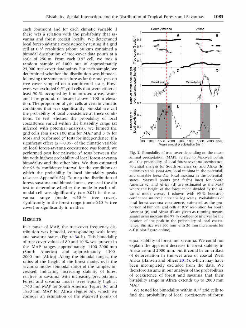
In a range of MAP, the tree-cover frequency dis-
tribution was bimodal, corresponding with forest
and savanna states (Figure 3a–b). This bimodality
of tree-cover values of 80 and 10 % was present in
the MAP ranges approximately 1100–2000 mm
(South America) and approximately 1300–
2000 mm (Africa). Along the bimodal ranges, the
ratios of the height of the forest modes over the
savanna modes (bimodal ratio) of the samples in-
creased, indicating increasing stability of forest
relative to savanna with increasing precipitation.
Forest and savanna modes were equally high at
1760 mm MAP for South America (Figure 3c) and
1580 mm MAP for Africa (Figure 3d), which we
consider an estimation of the Maxwell points of
equal stability of forest and savanna. We could not
explain the apparent decrease in forest stability in
Africa around 2000 mm, but it could be an artifact
of deforestation in the wet area of coastal West
Africa (Hansen and others 2013), which may have
been incompletely excluded from the data. We
therefore assume in our analysis of the probabilities
of coexistence of forest and savanna that their
bistability range in Africa extends up to 2000 mm
MAP.
We tested for bimodality within 0.5� grid cells to
find the probability of local coexistence of forest
Fig. 3. Bimodality of tree cover depending on the mean
annual precipitation (MAP), related to Maxwell points
and the probability of local forest-savanna coexistence.
Potential analysis for South America (a) and Africa (b)
indicates stable (solid dots, local minima in the potential)
and unstable (open dots, local maxima in the potential)
states. Maxwell points (red dashed lines) for South
America (c) and Africa (d) are estimated as the MAP
where the height of the forest mode divided by the sa-
vanna mode crosses 1 (shown with 95 % bootstrap
confidence interval; note the log scale). Probabilities of
local forest-savanna coexistence, estimated as the pro-
portion of bimodal grid cells at 0.5� resolution for South
America (e) and Africa (f) are given as running means.
Shaded areas indicate the 95 % confidence interval for the
location of the peak in the probability of local coexis-
tence. Bin size was 100 mm with 20 mm increments for
c–f (Color figure online)
Bistability, Spatial Interaction, and the Distribution of Tropical Forests and Savannas 1085

and savanna. For South America (Figure 3e), there
was a significant peak in the probability of local
coexistence between 1300 and 2000 mm MAP
(Appendix S2). This range contained the estimated
Maxwell point at 1760 mm MAP. For Africa (Fig-
ure 3f), the probability of local coexistence also
peaked significantly between 1500 and 2000 mm
MAP (Appendix S2). This range contained the
estimated Maxwell point at 1580 mm MAP.
Also in a range of Markham’s Seasonality Indices
(MSI, seasonality in precipitation), the tree-cover
frequency distribution sampled per continent was
bimodal (Figure 4a–b). This bimodality was present
in the MSI ranges 12–55 % (South America) and
12–35 % (Africa). Along the bimodal ranges, the
height of the forest mode over the savanna mode of
the samples decreased, indicating decreasing sta-
bility of forest relative to savanna with increasing
rainfall seasonality. These bimodal ratios crossed 1
at MSI = 50 % for South America (Figure 4c) and
at MSI = 24 % for Africa (Figure 4d), which we
considered estimations of Maxwell points of equal
stability of forest and savanna.
For South America (Figure 4e), there was a sig-
nificant peak in the probability of local coexistence
between MSI = 46–55 % (Appendix S2). This
range contained the estimated Maxwell point at
MSI = 50 %. For Africa (Figure 4f), the probability
of local coexistence did not peak significantly
within the inferred bistability range (Appendix S2).
Local coexistence of forest and savanna was
mostly found at boundaries of the Amazon and
Congo rainforests (Figure 5). We show the MAP
and MSI at these locations in Figure S3 and provide
Google Earth files of our results as Appendix S6.
DISCUSSION
Our results confirm that tropical forests and
savannas are bistable over a broad range of climatic
conditions (Hirota and others 2011; Staver and
others 2011b; Murphy and Bowman 2012). We
also found local coexistence of patches of forest and
savanna over a range of climatic conditions. How-
ever, the probability of local coexistence was not
always evenly distributed along the range of cli-
matic conditions at which we inferred bistability.
This effect can be interpreted in the light of
dynamical systems theory (Appendix S1; Van de
Leemput and others 2015), stating that spatial
interactions between patches narrow down the
range of conditions with stable coexistence of the
two states. Eventually, the most stable state would
dominate if we assume that local invasions of for-
ests and savannas are always possible and the sys-
tem is not dominated by stochasticity. Spatial
interactions between patches could thus eliminate
(part of) the hysteresis. If this is the case, we would
expect a significant decline of the probability of
forest-savanna coexistence further away from a
Maxwell point, even within the range of conditions
at which both states are stable when they are in
isolation. This effect becomes more pronounced
with increasing spatial interaction strength (Fig-
ure S2).
Within the range of MAP at which we inferred
bistability of forest and savanna, we observed a
Fig. 4. Bimodality of tree cover depending on rainfall
seasonality, related to Maxwell points and the probability
of local forest-savanna coexistence. Potential analysis for
South America (a) and Africa (b) indicates stable (solid
dots, local minima in the potential) and unstable (open
dots, local maxima in the potential) points. Maxwell
points (red dashed lines) for South America (c) and Africa
(d) are measured as the Markham’s Seasonality Index
(MSI) where the height of the forest mode divided by the
savanna mode crosses 1 (shown with 95 % bootstrap
confidence interval; note the log scale). Probabilities of
local forest-savanna coexistence, estimated as the pro-
portion of bimodal grid cells at 0.5� resolution for South
America (e) and Africa (f) are given as running means.
The shaded area in e indicates the 95 % confidence
interval for the location of the peak (there was no sig-
nificant effect in f). Bin size was 6 % with 1 % incre-
ments for c–f (Color figure online)
1086 A. Staal and others
significant effect of MAP on the probability of local
forest-savanna coexistence for both South America
and Africa. In the case of rainfall seasonality
(MSI), we observed a significant effect on local
coexistence only for South America. The climatic
conditions at which the probability of local coex-
istence peaked coincided with the conditions
where the forest and savanna modes in the tree-
cover frequency distribution were equally high.
Based on dynamical systems theory (Gilmore
1979; Gardiner 1985; Livina and others 2010), we
reason that such conditions correspond to the
Maxwell point, where two alternative states are
equally stable (Van de Leemput and others 2015;
Villa Martın and others 2015). We used a simple
model to illustrate the well-known principle
(Murray 2002) that if spatial interactions between
patches of two alternative stable states are very
strong relative to the states’ local self-stabilizing
mechanisms (that is, the Maxwell convention
applies to the system), then local coexistence of
the states under constant conditions is only
stable at the Maxwell point. However, in our
empirical results, the confidence intervals for the
peaks in the probability of local coexistence were
consistently wider than those for the Maxwell
points. Thus, the probability of local forest-sa-
vanna coexistence peaked at a wider range of
conditions than merely those at which the two
states were estimated to be equally stable.
There can be several explanations for the finding
that coexistence occurs at a wider range of condi-
tions than the Maxwell point (Appendix S5).
Firstly, it is possible that spatial interactions be-
tween patches are often too weak to establish the
most stable state; secondly, climatic conditions of
equal stability may differ between locations due to
other environmental factors; thirdly, fine-scale
spatial heterogeneity increases the occurrence of
coexistence; and fourthly, tree cover is often not in
equilibrium, due to either natural or human dis-
turbances.
The first explanation for the wider range of
conditions at which coexistence occurs implies
that we cannot fully confirm that the Maxwell
convention applies to tropical forests and savan-
nas. The results therefore do not refute that
transitions between the two states may occur at
tipping points.
The second explanation relates to the fact that
the Maxwell points that we determined represent
the average value for many locations. In reality,
stability of forest and savanna depends on other
environmental factors than only precipitation.
Therefore, variation in other relevant factors (such
as soil type) would also cause variation in the
Maxwell point for a certain climatic variable (such
as MAP). This variation in the environment would
also inflate our estimates of hysteresis and may
potentially give a false impression of alternative
stable states (and its prediction of sudden ecological
change) (Van Nes and others 2014).
The third explanation relates to local spatial
heterogeneity, which also expands the range of
climatic conditions at which local coexistence could
be found (Appendix S1; Favier and others 2004,
2012; Van Nes and Scheffer 2005). Examples of
such heterogeneity include local differences in
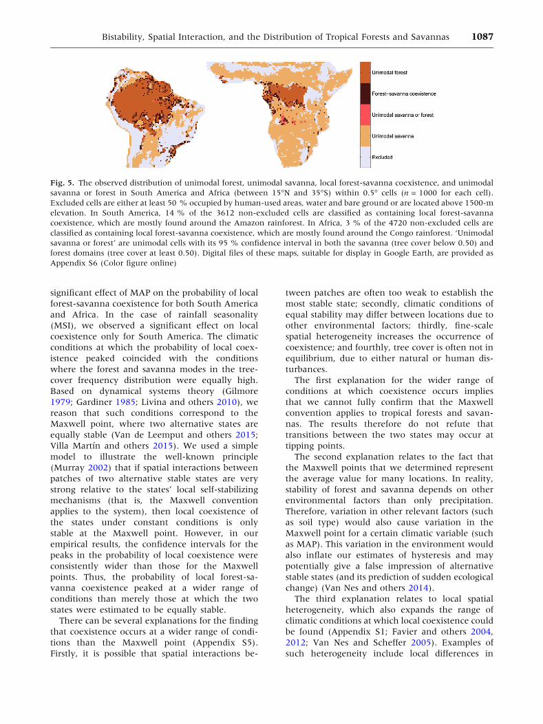
Fig. 5. The observed distribution of unimodal forest, unimodal savanna, local forest-savanna coexistence, and unimodal
savanna or forest in South America and Africa (between 15�N and 35�S) within 0.5� cells (n = 1000 for each cell).
Excluded cells are either at least 50 % occupied by human-used areas, water and bare ground or are located above 1500-m
elevation. In South America, 14 % of the 3612 non-excluded cells are classified as containing local forest-savanna
coexistence, which are mostly found around the Amazon rainforest. In Africa, 3 % of the 4720 non-excluded cells are
classified as containing local forest-savanna coexistence, which are mostly found around the Congo rainforest. ‘Unimodal
savanna or forest’ are unimodal cells with its 95 % confidence interval in both the savanna (tree cover below 0.50) and
forest domains (tree cover at least 0.50). Digital files of these maps, suitable for display in Google Earth, are provided as
Appendix S6 (Color figure online)
Bistability, Spatial Interaction, and the Distribution of Tropical Forests and Savannas 1087
water availability, differential responses of species
to water stress and differences in soil properties
(Levine and others 2016). Examples include gallery
forests, which occur in savanna landscapes where
local water availability is high. Environmental
variability on a scale in the order of the tree-cover
data (250 m) could thus deterministically cause
local bimodality of tree cover. However, there is
also evidence that local heterogeneity in soils may
be enhanced by the vegetation itself and therefore
be not only cause, but also effect of vegetation
patchiness. It has, for instance, been shown that
expansion of forest trees over savannas and grass-
lands increases soil fertility (Silva and others 2008;
Silva and Anand 2011; Paiva and others 2015).
More fertile soils in turn favor the development of a
closed canopy, which suppresses fire (Hoffmann
and others 2012). Thus, a positive feedback be-
tween forest trees and soil fertility may reinforce
forest-savanna bistability (Hoffmann and others
2012; Silva and others 2013; Staal and Flores 2015)
and therefore enhance coexistence in the absence
of predetermined environmental heterogeneity.
The fourth explanation is that the distribution of
forests and savannas is often not in equilibrium,
because these systems are dynamic and always
subject to disturbances. These disturbances can not
only be anthropogenic (such as deforestation,
which has been imperfectly excluded from the
data) but also natural. The latter is indicated, for
instance, by the large variability in tree cover ob-
served both in the field and from satellites (Fig-
ure S4; Sankaran and others 2005; Hirota and
others 2011; Ratajczak and Nippert 2012; Van Nes
and others 2012). Stochasticity may occasionally
push the system away from the most stable state
and can thus be expected to expand the range of
climatic conditions at which forest-savanna coex-
istence is found. The closer conditions are to the
Maxwell point, the longer it takes for a system to
move to its equilibrium (Scheffer and others 2015b;
Van de Leemput and others 2015). Thus, even
when forest and savanna can be alternative
stable states, part of the forest-savanna coexistence
we observe may be transient ecosystem configu-
rations. Note, however, that these effects of tem-
poral as well as spatial variability in conditions do
not affect whether or not the probability of coex-
istence differs within inferred bistability ranges.
In South America, the effects of MAP and MSI on
the probability of local forest-savanna coexistence
within the inferred bistability ranges were both
strongly significant, whereas in Africa only MAP
had an effect and it was weakly significant. The
weak correspondence between climate and forest-
savanna coexistence in Africa could relate to any of
the four explanations listed above. However, we
conjecture that in Africa there are weak spatial
interactions between forest and savanna patches
relative to the local self-stabilizing mechanisms of
these patches (Appendix S1). Specifically, the
growth of grasses is faster and responds more
strongly to MAP in Africa than in South America
(Lehmann and others 2014). Indeed, fire frequen-
cies are higher in Africa than in South America
(Lehmann and others 2011). We therefore
hypothesize that the grass-fire feedback is faster in
African savannas than in South American ones,
which could explain why we found that forest-sa-
vanna boundaries more strongly follow the Max-
well point in South America. There, the estimated
Maxwell point for MSI coincided very well with the
independently observed peak in the probability of
local forest-savanna coexistence. This peak was also
more narrow and pronounced for MSI than for
MAP, which suggests that rainfall seasonality more
strongly affects the South American forest-savanna
distribution than average rainfall does. By contrast,
our results suggest that average rainfall more
strongly affects the African forest-savanna distri-
bution than rainfall seasonality does. This contrast
resonates with the yet unanswered question why
savannas in South America can persist under wet-
ter conditions than in Africa (Lehmann and others
2014). Part of the explanation can be that African
forests are better adapted to dry conditions than
South American ones. Indeed, analyses of satellite
radar data, which can indicate canopy mortality,
showed that African forests are resilient against
occasional drought (Asefi-Najafabady and Saatchi
2013), whereas Amazon forests have higher
drought sensitivity (Saatchi and others 2013).
Most cases of local forest-savanna coexistence
that we observed occurred at the boundaries of the
Amazon and Congo rainforests, whereas it was
relatively rare at other locations. This is consistent
with the modeling result that local coexistence of
forests and savannas is not always stable, even in
the inferred bistability range. However, it is possible
that our conservative approach in detecting statis-
tically significant bimodality on the basis of 0.5�grid cells has contributed to its scarcity. Further-
more, many 0.5� cells in the Brazilian savanna
(‘cerrado’) were excluded from the analysis due to
human impacts, which may have caused an
underestimation of the occurrence of local forest-
savanna coexistence in this region. On the other
hand, we may have included human impacted
areas at the boundaries of the rainforests and thus
overestimated the coexistence at these boundaries.
1088 A. Staal and others
Local forest-savanna coexistence was about twice
as probable in South America as in Africa. This may
have been caused by a difference in the size of the
continents’ major rainforest, as the circumference
of the Amazon relative to the area of South
America is about twice as large as the circumfer-
ence of the Congo forest relative to the area of
Africa.
We have presented a novel way of identifying
the relative stability of forests and savannas,
building upon modeling results (Appendix S1; Van
de Leemput and others 2015; Villa Martın and
others 2015). The climatic conditions of average
equal stability, at which a boundary between
alternative stable states in theory stabilizes, can be
detected from peak heights in bimodal frequency
distributions of tree cover sampled on a continental
scale. This differs from the definition of resilience
by Hirota and others (2011). According to that
definition, resilience of a state is the probability
that an observation of tree cover falls in the state’s
basin of attraction, where the cut-off between sa-
vanna and forest was set at 60 % tree cover. Our
approach does not require the definition of a cut-
off between basins of attraction for inferring sta-
bility.
In summary, our results support previous stud-
ies that have suggested that tropical forests and
savannas can be alternative stable states, thereby
opposing climate determinism in the distribution
of these biomes (for example, Hirota and others
2011; Staver and others 2011a; Staver and others
2011b; Favier and others 2012; Murphy and
Bowman 2012; Staal and Flores 2015). Thus, our
results indicate that changes in precipitation re-
gimes could cause spatial shifts of the boundaries
between forests and savannas when tipping points
are crossed. However, both theoretical and
empirical results of our study also indicate that
forests and savannas may have less hysteresis than
suggested by previous studies, which did not ac-
count for spatial interactions between patches of
the two alternative stable states. An implication of
our results is then that invasion of a low tree-
cover state into a forest, facilitated for instance by
logging, could cause the spread of a savanna-like
landscape into the forest. Thus, understanding and
preventing forest-savanna transitions requires the
consideration of different scales, as changes in
climate and in tree cover could together cross
critical points (Staal and others 2015) after which
undesirable biome shifts become inevitable (Sch-
effer and others 2015a).
ACKNOWLEDGEMENTS
We thank Bernardo M. Flores, two anonymous
reviewers, Niall P. Hanan and Brandon T. Bes-
telmeyer for useful comments on the manuscript.
AS is grateful to Johan Cruijff for his ‘‘momentos
dados.’’ AS is supported by a PhD scholarship
‘‘Complex dynamics in human-environment sys-
tems’’ from SENSE Research School. CX is sup-
ported by the National Natural Science Foundation
of China (41271197). EHvN is supported by an ERC
advanced grant awarded to Marten Scheffer. This
work was carried out under the program of the
Netherlands Earth System Science Center (NESSC).
OPEN ACCESS
This article is distributed under the terms of the
Creative Commons Attribution 4.0 International
License (http://creativecommons.org/licenses/by/
4.0/), which permits unrestricted use, distribution,
and reproduction in any medium, provided you
give appropriate credit to the original author(s) and
the source, provide a link to the Creative Commons
license, and indicate if changes were made.
REFERENCES
Asefi-Najafabady S, Saatchi S. 2013. Response of African humid
tropical forests to recent rainfall anomalies. Philos Trans R Soc
B 368:20120306.
Bel G, Hagberg A, Meron E. 2012. Gradual regime shifts in
spatially extended ecosystems. Theor Ecol 5:591–604.
Bond WJ. 2008. What limits trees in C4 grasslands and savan-
nas? Ann Rev Ecol Evol Syst 39:641–59.
Bowman DMJS, Perry GLW, Marston JB. 2015. Feedbacks and
landscape-level vegetation dynamics. Trends Ecol Evol
30:255–60.
Brando PM, Balch JK, Nepstad DC, Morton DC, Putz FE, Coe
MT, Silverio D, Macedo MN, Davidson EA, Nobrega CC,
Alencar A, Soares-Filho BS. 2014. Abrupt increases in Ama-
zonian tree mortality due to drought–fire interactions. Proc
Natl Acad Sci 111:6347–52.
Carpenter SR, Cole JJ, Pace ML, Batt R, Brock W, Cline T, Coloso
J, Hodgson JR, Kitchell JF, Seekell DA. 2011. Early warnings
of regime shifts: a whole-ecosystem experiment. Science
332:1079–82.
Dai L, Korolev KS, Gore J. 2013. Slower recovery in space before
collapse of connected populations. Nature 496:355–8.
Dantas VL, Batalha MA, Pausas JG. 2013. Fire drives functional
thresholds on the savanna-forest transition. Ecology 94:2454–
63.
Dantas VL, Hirota M, Oliveira RS, Pausas JG. 2016. Disturbance
maintains alternative biome states. Ecol Lett 19:12–19.
DiMiceli CM, Carroll ML, Sohlberg RA, Huang C, Hansen MC,
Townshend JRG. 2011. Annual global automated MODIS
Bistability, Spatial Interaction, and the Distribution of Tropical Forests and Savannas 1089
vegetation continuous fields (MOD44B) at 250 m spatial reso-
lution for data years beginning day 65, 2000–2010, collection 5
percent tree cover. College Park, MD: University of Maryland.
Favier C, Aleman J, Bremond L, Dubois MA, Freycon V, Yan-
gakola JM. 2012. Abrupt shifts in African savanna tree cover
along a climatic gradient. Glob Ecol Biogeogr 21:787–97.
Favier C, Chave J, Fabing A, Schwartz D, Dubois MA. 2004.
Modelling forest–savanna mosaic dynamics in man-influ-
enced environments: effects of fire, climate and soil hetero-
geneity. Ecol Modell 171:85–102.
Fort H. 2013. Statistical mechanics ideas and techniques applied
to selected problems in ecology. Entropy 15:5237–76.
Gardiner C. 1985. Stochastic methods. Berlin: Springer.
Gilmore R. 1979. Catastrophe time scales and conventions. Phys
Rev A 20:2510–15.
Gilmore R. 1981. Catastrophe theory for scientists and engi-
neers. New York: Wiley.
Goetze D, Horsch B, Porembski S. 2006. Dynamics of forest-
savanna mosaics in north-eastern Ivory Coast from 1954 to
2002. J Biogeogr 33:653–64.
Hanan NP, Tredennick AT, Prihodko L, Bucini G, Dohn J. 2014.
Analysis of stable states in global savannas: is the CART
pulling the horse? Glob Ecol Biogeogr 23:259–63.
Hanan NP, Tredennick AT, Prihodko L, Bucini G, Dohn J. 2015.
Analysis of stable states in global savannas—a response to
Staver and Hansen. Glob Ecol Biogeogr 24:988–9.
Hansen MC, Potapov PV, Moore R, Hancher M, Turubanova SA,
Tyukavina A, Thau D, Stehman SV, Goetz SJ, Loveland TR.
2013. High-resolution global maps of 21st-century forest
cover change. Science 342:850–3.
Hartigan JA, Hartigan PM. 1985. The dip test of unimodality.
Ann Stat 13:70–84.
Hijmans RJ, Cameron SE, Parra JL, Jones PG, Jarvis A. 2005.
Very high resolution interpolated climate surfaces for global
land areas. Int J Climatol 25:1965–78.
Hirota M, Holmgren M, van Nes EH, Scheffer M. 2011. Global
resilience of tropical forest and savanna to critical transitions.
Science 334:232–5.
Hoffmann WA, Geiger EL, Gotsch SG, Rossatto DR, Silva LCR,
Lau OL, Haridasan M, Franco AC. 2012. Ecological thresholds
at the savanna-forest boundary: how plant traits, resources
and fire govern the distribution of tropical biomes. Ecol Lett
15:759–68.
Keeley JE, Pausas JG, Rundel PW, Bond WJ, Bradstock RA.
2011. Fire as an evolutionary pressure shaping plant traits.
Trends Plant Sci 16:406–11.
Lehmann CER, Anderson TM, Sankaran M, Higgins SI, Archi-
bald S, Hoffmann WA, Hanan NP, Williams RJ, Fensham RJ,
Felfili J, Hutley LB, Ratnam J, San Jose J, Montes R, Franklin
D, Russell-Smith J, Ryan CM, Durigan G, Hiernaux P, Haidar
R, Bowman DMJS, Bond WJ. 2014. Savanna vegetation-fire-
climate relationships differ among continents. Science
343:548–52.
Lehmann CER, Archibald SA, Hoffmann WA, Bond WJ. 2011.
Deciphering the distribution of the savanna biome. New
Phytol 191:197–209.
Levine NM, Zhang K, Longo M, Baccini A, Phillips OL, Lewis SL,
Alvarez-Davila E, Segalin de Andrade AC, Brienen RJW, Er-
win TL, Feldpausch TR, Monteagudo Mendoza AL, Nunez
Vargaz P, Prieto A, Silva-Espejo JE, Malhi Y, Moorcroft PR.
2016. Ecosystem heterogeneity determines the ecological re-
silience of the Amazon to climate change. Proc Natl Acad Sci
113:793–7.
Livina VN, Kwasniok F, Lenton TM. 2010. Potential analysis
reveals changing number of climate states during the last 60
kyr. Clim Past 6:77–82.
Markham CG. 1970. Seasonality of precipitation in the United
States. Ann Assoc Am Geogr 60:593–7.
Maxwell JC. 1875. On the dynamical evidence of the molecular
constitution of bodies. Nature 11:357–9.
Mitchell TD, Jones PD. 2005. An improved method of con-
structing a database of monthly climate observations and
associated high-resolution grids. Int J Climatol 25:693–712.
Moncrieff GR, Bond WJ, Higgins SI. 2016. Revising the biome
concept for understanding and predicting global change im-
pacts. J Biogeogr 43:863–873.
Murphy BP, Bowman DMJS. 2012. What controls the distribu-
tion of tropical forest and savanna? Ecol Lett 15:748–58.
Murray JD. 2002. Mathematical biology: I. An introduction. 3rd
edn. Berlin: Springer.
Noy-Meir I. 1975. Stability of grazing systems: an application of
predator-prey graphs. J Ecol 63:459–81.
Paiva AO, Silva LCR, Haridasan M. 2015. Productivity-efficiency
tradeoffs in tropical gallery forest-savanna transitions: linking
plant and soil processes through litter input and composition.
Plant Ecol 216:775–87.
Pomeau Y. 1986. Front motion, metastability and subcritical
bifurcations in hydrodynamics. Physica D 23:3–11.
Ratajczak Z, Nippert JB. 2012. Comment on ‘‘Global resilience of
tropical forest and savanna to critical transitions’’. Science
336: 541-c.
Reyer CPO, Brouwers N, Rammig A, Brook BW, Epila J, Grant
RF, Holmgren M, Langerwisch F, Leuzinger S, Lucht W,
Medlyn B, Pfeifer M, Steinkamp J, Vanderwel MC, Verbeeck
H, Villela DM. 2015. Forest resilience and tipping points at
different spatio-temporal scales: approaches and challenges. J
Ecol 103:5–15.
Saatchi S, Asefi-Najafabady S, Malhi Y, Aragao LE, Anderson
LO, Myneni RB, Nemani R. 2013. Persistent effects of a severe
drought on Amazonian forest canopy. Proc Natl Acad Sci
110:565–70.
Sankaran M, Hanan NP, Scholes RJ, Ratnam J, Augustine DJ,
Cade BS, Gignoux J, Higgins SI, Le Roux X, Ludwig F, Ardo J,
Banyikwa F, Bronn A, Bucini G, Caylor KK, Coughenour MB,
Diouf A, Ekaya W, Feral CJ, February EC, Frost PGH, Hier-
naux P, Hrabar H, Metzger KL, Prins HHT, Ringrose S, Sea W,
Tews J, Worden J, Zambatis N. 2005. Determinants of woody
cover in African savannas. Nature 438:846–9.
Scheffer M. 2009. Critical transitions in nature and society.
Princeton: Princeton University Press.
Scheffer M, Barrett S, Carpenter SR, Folke C, Green AJ, Holmgren
M, Hughes TP, Kosten S, van de Leemput IA, Nepstad DC, van
Nes EH, Peeters ETHM, Walker B. 2015a. Creating a safe oper-
ating space for iconic ecosystems. Science 347:1317–19.
Scheffer M, Carpenter SR, Dakos V, van Nes E. 2015b. Generic
indicators of ecological resilience: inferring the chance of a
critical transition. Ann Rev Ecol Evol Syst 46:145–67.
Scheffer M, Carpenter S, Foley JA, Folke C, Walker B. 2001.
Catastrophic shifts in ecosystems. Nature 413:591–6.
Scheffer M, Carpenter SR. 2003. Catastrophic regime shifts in
ecosystems: linking theory to observation. Trends Ecol Evol
18:648–56.
1090 A. Staal and others
Schimper AFW. 1903. Plant-geography upon a physiological
basis. Oxford: Clarendon Press.
Silva LCR, Anand M. 2011. Mechanisms of Araucaria (Atlantic)
forest expansion into southern Brazilian grasslands. Ecosys-
tems 14:1354–71.
Silva LCR, Hoffmann WA, Rossatto DR, Haridasan M, Franco
AC, Horwath WR. 2013. Can savannas become forests? A
coupled analysis of nutrient stocks and fire thresholds in
central Brazil. Plant Soil 373:829–42.
Silva LCR, Sternberg L, Haridasan M, Hoffmann WA, Miralles-
Wilhelm F, Franco AC. 2008. Expansion of gallery forests into
central Brazilian savannas. Glob Change Biol 14:2108–18.
Silverman BW. 1986. Density estimation for statistics and data
analysis. Boca Raton: CRC Press.
Staal A, Dekker SC, Hirota M, van Nes EH. 2015. Synergistic
effects of drought and deforestation on the resilience of the
south-eastern Amazon rainforest. Ecol Complex 22:65–75.
Staal A, Flores BM. 2015. Sharp ecotones spark sharp ideas:
comment on ‘‘Structural, physiognomic and above-ground
biomass variation in savanna-forest transition zones on three
continents—how different are co-occurring savanna and for-
est formations?’’ by Veenendaal and others (2015). Biogeo-
sciences 12:5563–6.
Staver AC, Archibald S, Levin S. 2011a. Tree cover in sub-Sa-
haran Africa: rainfall and fire constrain forest and savanna as
alternative stable states. Ecology 92:1063–72.
Staver AC, Archibald S, Levin SA. 2011b. The global extent and
determinants of savanna and forest as alternative biome
states. Science 334:230–2.
Staver AC, Hansen MC. 2015. Analysis of stable states in global
savannas: is the CART pulling the horse?–a comment. Glob
Ecol Biogeogr 24:985–7.
Strogatz SH. 1994. Nonlinear dynamics and chaos: with appli-
cations to physics, biology and chemistry. New York: Perseus
Publishing.
Van de Leemput IA, van Nes EH, Scheffer M. 2015. Resilience of
alternative states in spatially extended ecosystems. PloS One
10:e0116859.
Van Nes EH, Hirota M, Holmgren M, Scheffer M. 2014. Tipping
points in tropical tree cover: linking theory to data. Glob
Change Biol 20:1016–21.
Van Nes EH, Holmgren M, Hirota M, Scheffer M. 2012. Response
to comment on ‘‘Global resilience of tropical forest and sa-
vanna to critical transitions’’. Science 336: 541-d.
Van Nes EH, Scheffer M. 2005. Implications of spatial hetero-
geneity for catastrophic regime shifts in ecosystems. Ecology
86:1797–807.
Villa Martın P, Bonachela JA, Levin SA, Munoz MA. 2015.
Eluding catastrophic shifts. Proc the Natl Acad Sci 112:E1828–
36.
Von Humboldt A, Bonpland A. 1807. Essay on the geography of
plants: 2009 reissue. Chicago: University of Chicago Press.
Wilson WG, Nisbet RM, Ross AH, Robles C, Desharnais RA.
1996. Abrupt population changes along smooth environ-
mental gradients. Bull Math Biol 58:907–22.
Xu C, Holmgren M, van Nes EH, Hirota M, Chapin FS III, Sch-
effer M. 2015. A changing number of alternative states in the
boreal biome: reproducibility risks of replacing remote sensing
products. PloS One 10:e0143014.
Zhang C, Mapes BE, Soden BJ. 2003. Bimodality in tropical
water vapour. Q J R Meteorol Soc 129:2847–66.
Bistability, Spatial Interaction, and the Distribution of Tropical Forests and Savannas 1091
Top Related