1

Biased Normalized Cuts

Subhransu Maji and Jithndra MalikUniversity of California, Berkeley

IEEE Conference on Computer Vision and Pattern Recognition (IEEE CVPR 2011)

Poster

Nisheeth K. VishnoiMiscrosoft Research India, Bangalore

2

Outline• Review of ‘Normalized Cuts’

• Introduction to ‘Biased Normalized Cuts’

• Biased Graph Partitioning

• Algorithm

• Qualitative Evaluation

3

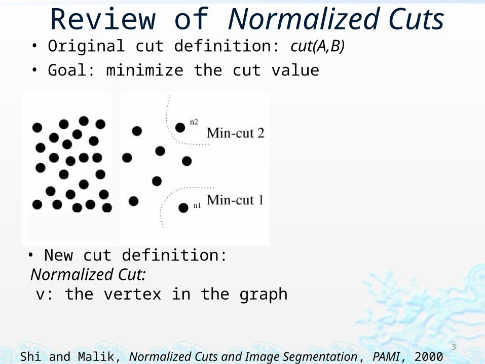
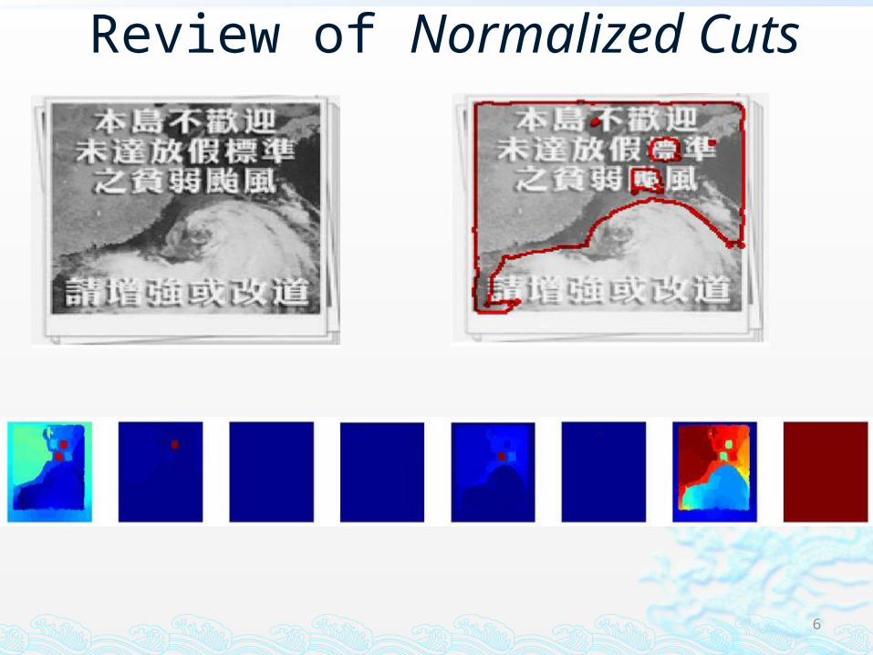
Review of Normalized Cuts

• New cut definition: Normalized Cut: v: the vertex in the graph

Shi and Malik, Normalized Cuts and Image Segmentation, PAMI, 2000

• Goal: minimize the cut value

• Original cut definition: cut(A,B)

4

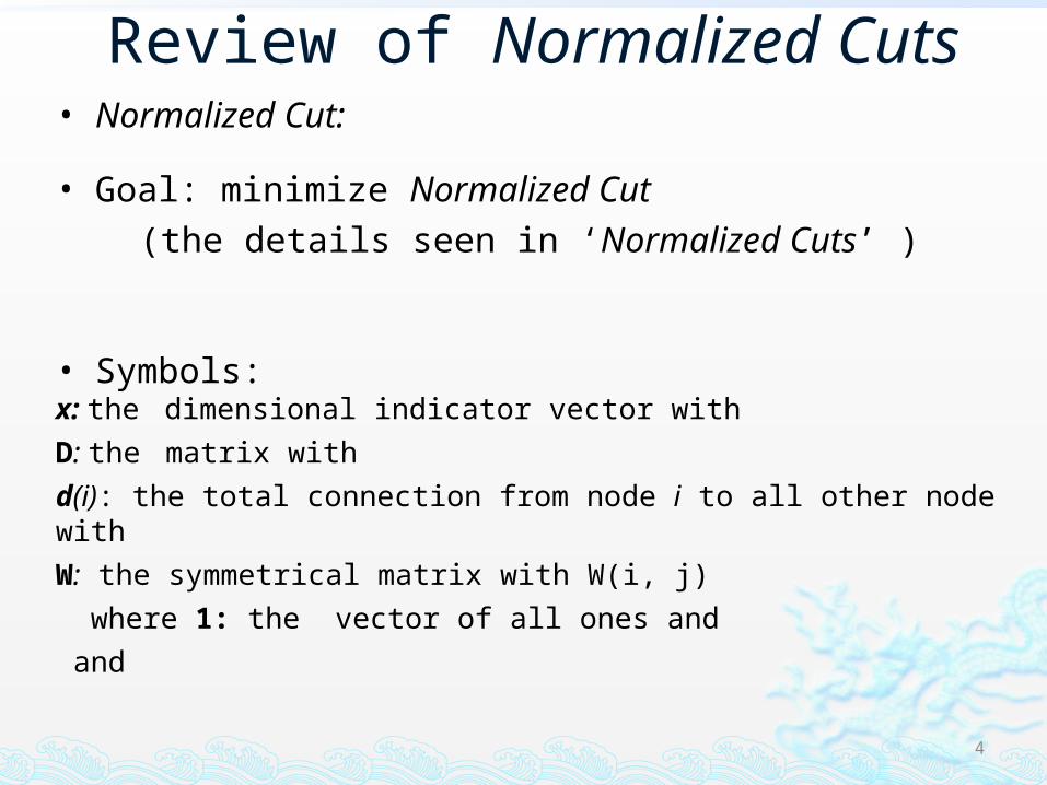
Review of Normalized Cuts• Normalized Cut:

• Goal: minimize Normalized Cut

(the details seen in ‘Normalized Cuts’ )

• Symbols:x: the dimensional indicator vector with

D: the matrix with

d(i): the total connection from node i to all other node with

W: the symmetrical matrix with W(i, j)

where 1: the vector of all ones and

and

5

Review of Normalized Cuts

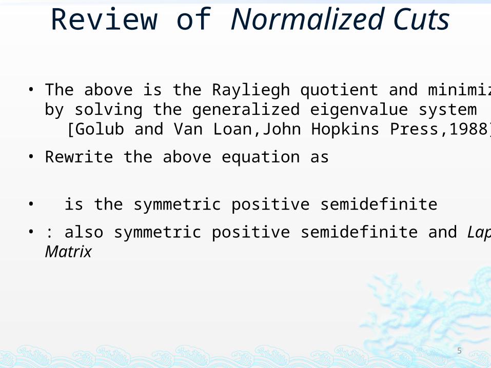
• The above is the Rayliegh quotient and minimize it by solving the generalized eigenvalue system

[Golub and Van Loan,John Hopkins Press,1988]

• Rewrite the above equation as

• is the symmetric positive semidefinite

• : also symmetric positive semidefinite and Laplacian Matrix

6

Review of Normalized Cuts

7

Introduction to ‘Biased Normalized Cuts’

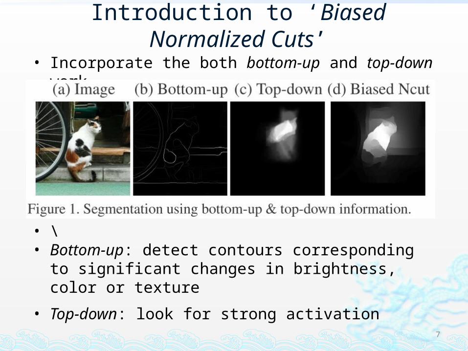
• Incorporate the both bottom-up and top-down work

• \• Bottom-up: detect contours corresponding to significant

changes in brightness, color or texture

• Top-down: look for strong activation　

8

Introduction to ‘Biased Normalized Cuts’

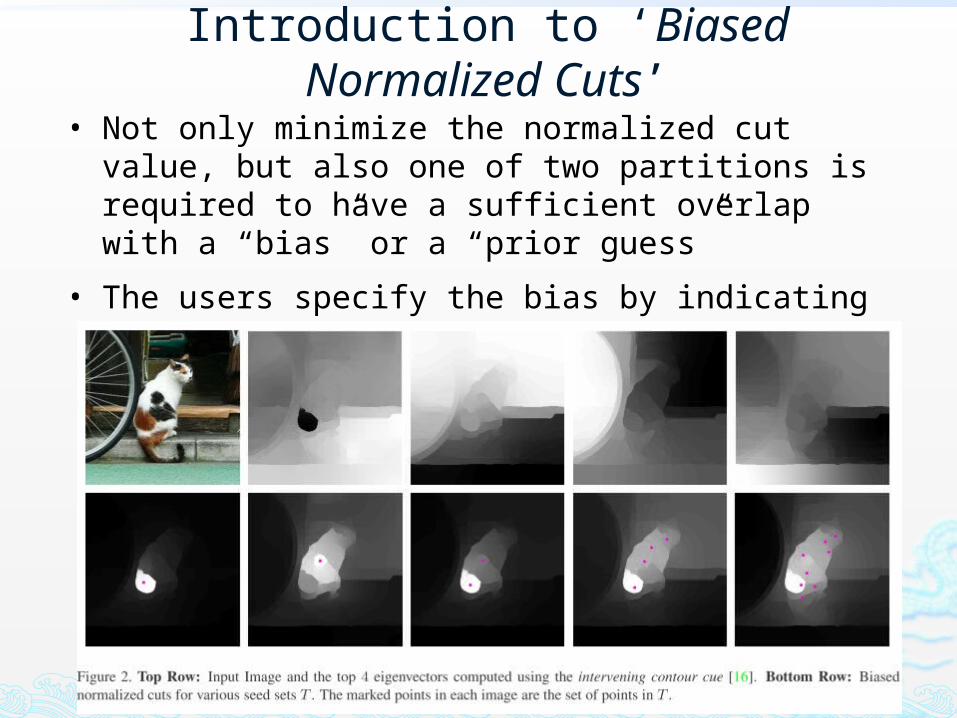
• Not only minimize the normalized cut value, but also one of two partitions is required to have a sufficient overlap with a “bias” or a “prior guess”

• The users specify the bias by indicating various point set T with a seed-vector

9

Introduction to ‘Biased Normalized Cuts’

• Two advantages:1. Solutions which are sufficiently “correlated” with priors which

allows us to use noisy top-down information

2. Given the spectral solution of the unconstrained problem, the solution of the constrained one can be computed in small additional time, which allows to run the algorithm in an interactive mode

10

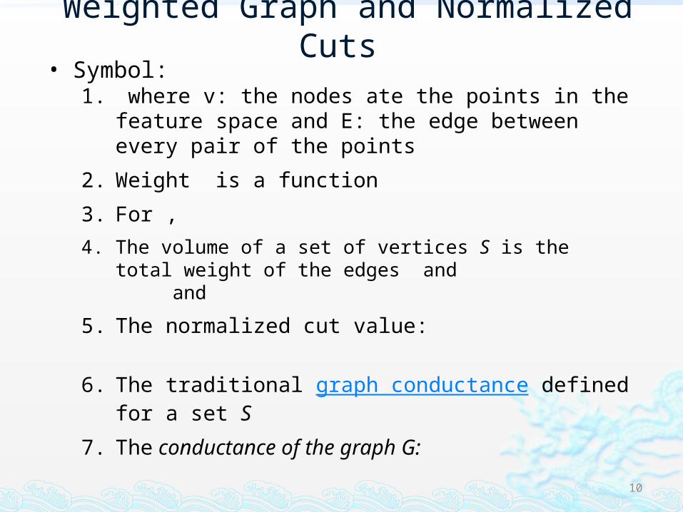
Weighted Graph and Normalized Cuts • Symbol:

1. where v: the nodes ate the points in the feature space and E: the edge between every pair of the points

2. Weight is a function

3. For ,

4. The volume of a set of vertices S is the total weight of the edges and and

5. The normalized cut value:

6. The traditional graph conductance defined for a set S

7. The conductance of the graph G:

11

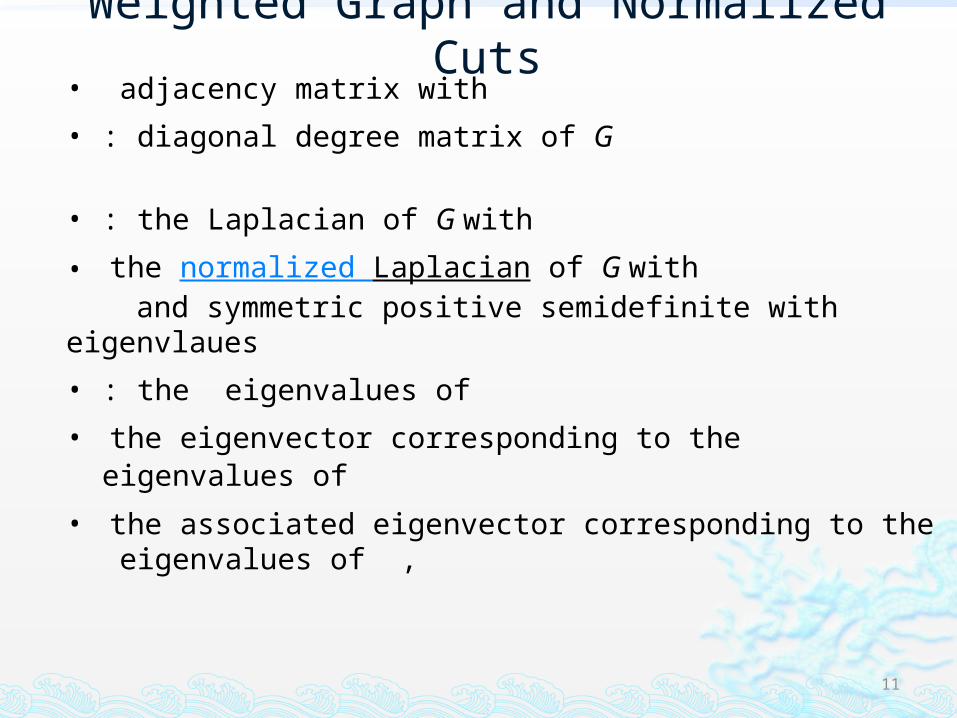
Weighted Graph and Normalized Cuts• adjacency matrix with

• : diagonal degree matrix of G

• : the Laplacian of G with

• the normalized Laplacian of G with and symmetric positive semidefinite with eigenvlaues

• : the eigenvalues of

• the eigenvector corresponding to the eigenvalues of

• the associated eigenvector corresponding to the eigenvalues of ,

12

The Spectral Relaxation to Computing Normalized Cuts

• Approximate the solution by minimizing subject to

•

•

13

Biased Normalized Cuts

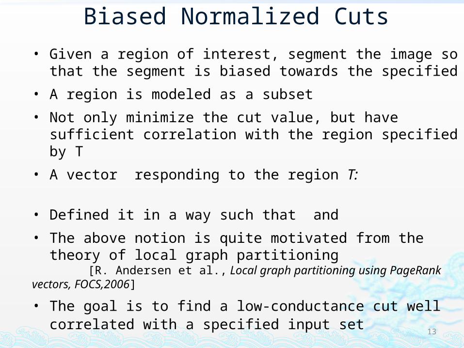
• Given a region of interest, segment the image so that the segment is biased towards the specified

• A region is modeled as a subset

• Not only minimize the cut value, but have sufficient correlation with the region specified by T

• A vector responding to the region T:

• Defined it in a way such that and

• The above notion is quite motivated from the theory of local graph partitioning

[R. Andersen et al., Local graph partitioning using PageRank vectors, FOCS,2006]

• The goal is to find a low-conductance cut well correlated with a specified input set

14

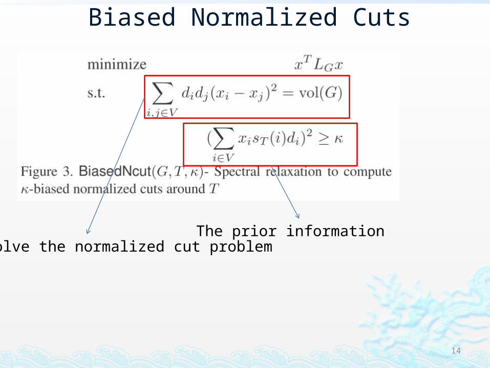
Biased Normalized Cuts

Solve the normalized cut problemThe prior information

15

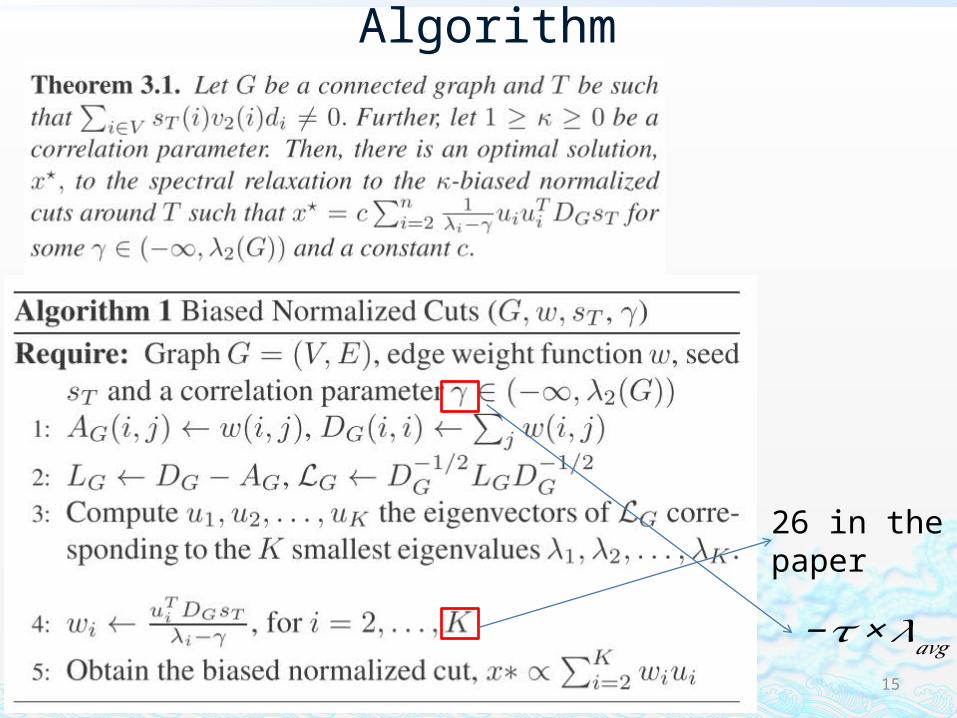
Algorithm

26 in the paper

−𝜏× 𝜆𝑎𝑣𝑔

16

Qualitative Evaluation

• Use the PASCAL VOC 2010 dataset

• Weight matrix: use the intervening contour cue [M. Maire et al., Using contours to detect and localize junctions in natural images, CVPR, 2008]

17

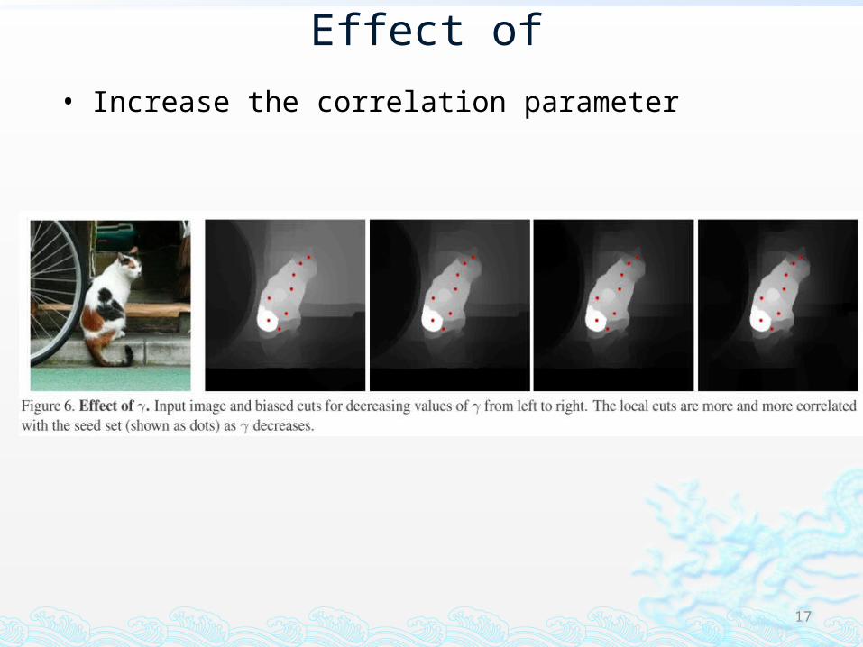
Effect of

• Increase the correlation parameter

18

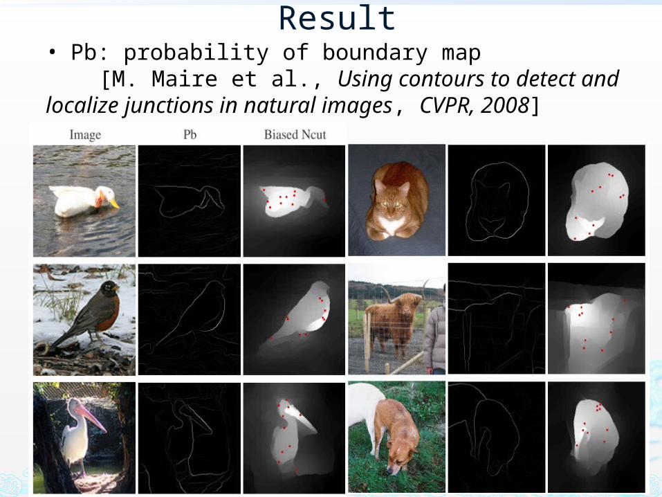
Result• Pb: probability of boundary map [M. Maire et al., Using contours to detect and localize junctions in natural images, CVPR, 2008]

19

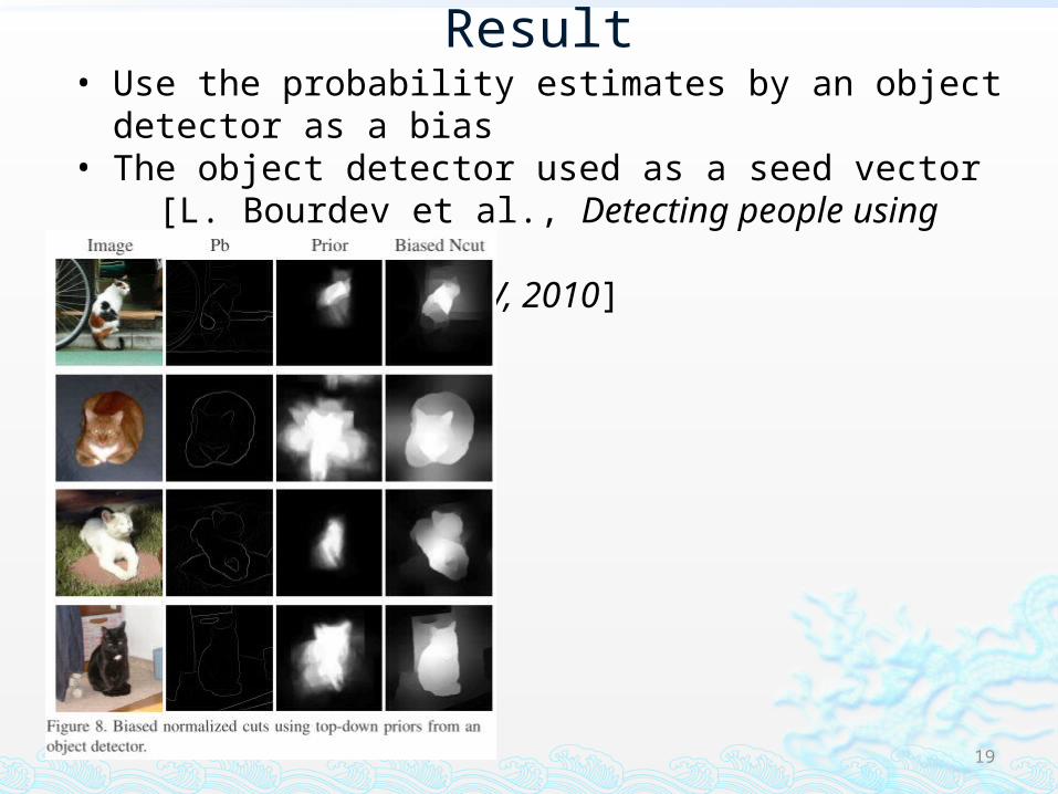
Result• Use the probability estimates by an object detector as a bias • The object detector used as a seed vector [L. Bourdev et al., Detecting people using mutually consistent poselet activations, ECCV, 2010]