


Languages
Pages
Legal


Bayesian Models for Radio Bayesian Models for Radio Telemetry Habitat DataTelemetry Habitat Data
Megan C. Dailey*Megan C. Dailey*Alix I. GitelmanAlix I. GitelmanFred L. RamseyFred L. RamseySteve StarcevichSteve Starcevich
* * Department of Statistics, Colorado State UniversityDepartment of Statistics, Colorado State UniversityDepartment of Statistics, Oregon State UniversityDepartment of Statistics, Oregon State University
Oregon Department of Fish and WildlifeOregon Department of Fish and Wildlife
†
‡
†
†
‡

Affiliations and fundingAffiliations and funding
FUNDING/DISCLAIMERThe work reported here was developed under the STAR Research Assistance Agreement CR-829095
awarded by the U.S. Environmental Protection Agency (EPA) to Colorado State University. This poster
has not been formally reviewed by EPA. The views expressed here are solely those of the authors and
STARMAP, the Program they represent. EPA does not endorse any products or commercial services
mentioned in this presentation.
CR-829095

Westslope Cutthroat TroutWestslope Cutthroat Trout Year long radio-telemetry study (Year long radio-telemetry study (Steve Starcevich)Steve Starcevich)
• 2 headwater streams of the John Day River in eastern 2 headwater streams of the John Day River in eastern OregonOregon
• 26 trout were tracked ~ weekly from stream side26 trout were tracked ~ weekly from stream side Roberts CreekRoberts Creek F = 17F = 17 Rail CreekRail Creek F = 9F = 9
• Winter, Spring, Summer (2000-2001)Winter, Spring, Summer (2000-2001) S=3S=3

Habitat associationHabitat association Habitat inventory of entire creek once per seasonHabitat inventory of entire creek once per season
• Channel unit typeChannel unit type• Structural association of poolsStructural association of pools• Total area of each habitat typeTotal area of each habitat type
For this analysis: For this analysis: • H = 3 habitat classesH = 3 habitat classes
1.1. In-stream-large-wood pool (ILW)In-stream-large-wood pool (ILW)
2.2. Other pool (OP)Other pool (OP)
3.3. Fast water (FW)Fast water (FW)
• Habitat availability = total area of habitat in creekHabitat availability = total area of habitat in creek

Goals of habitat analysisGoals of habitat analysis IncorporateIncorporate
– multiple seasonsmultiple seasons– multiple streamsmultiple streams– Other covariatesOther covariates
Investigate “Use vs. Availability”Investigate “Use vs. Availability”

Radio telemetry dataRadio telemetry data Sequences of observed habitat useSequences of observed habitat use
SUMMERWINTER SPRING
FISH 2
FISH 1
Habitat 1 Habitat 3Habitat 2 missing
2,2,1,3,3,3,3,3,1,1,3,3,1,1,3,3,3,0winter,2 sfX
2,2,3,3,3,3,1,3,3,1,3,3,3,3,3,3,3,3winter,1 sfX
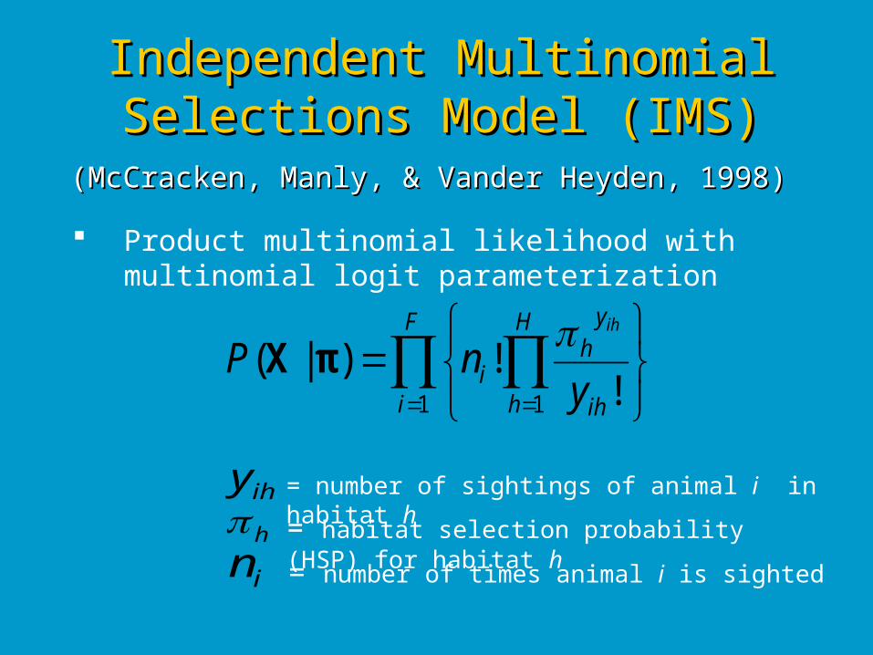
Independent Multinomial Selections Independent Multinomial Selections Model (IMS)Model (IMS)
(McCracken, Manly, & Vander Heyden, 1998)(McCracken, Manly, & Vander Heyden, 1998)
Product multinomial likelihood with multinomial logit parameterization
F
i
H
h ih
yh
i ynP
ih
1 1 !!)|(
πX
= number of sightings of animal i in habitat hihy
h = habitat selection probability (HSP) for habitat h
= number of times animal i is sightedin
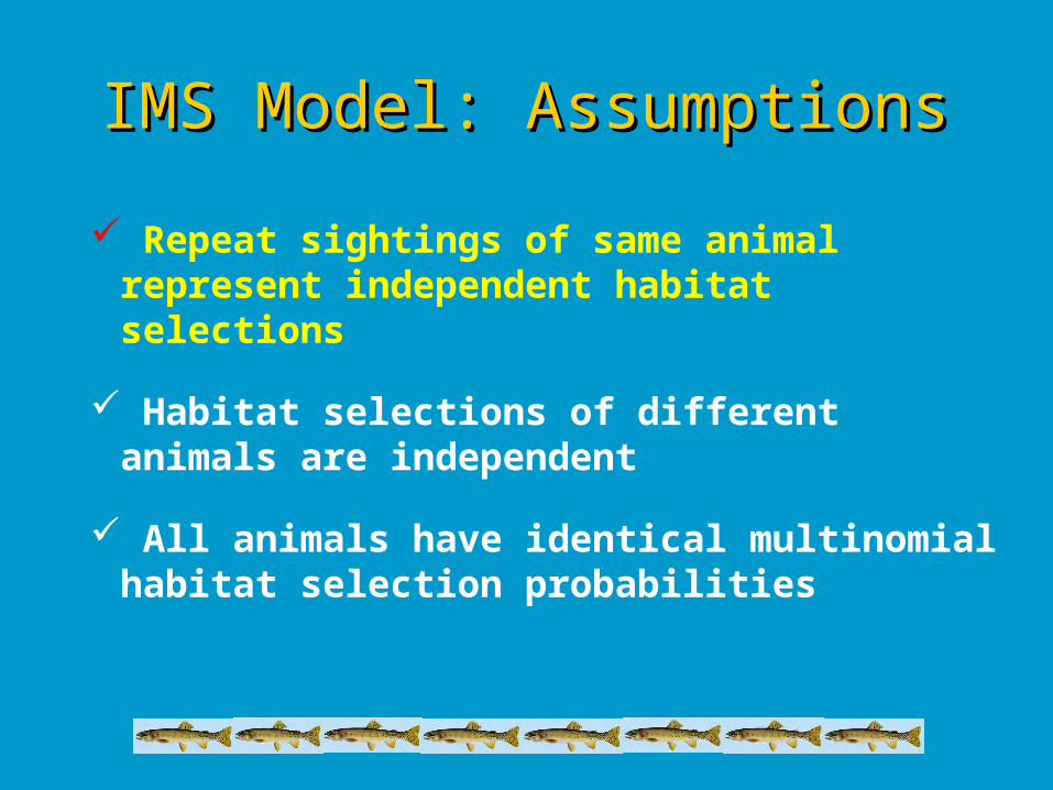
IMS Model: AssumptionsIMS Model: Assumptions
Repeat sightings of same animal represent independent habitat selections
Habitat selections of different animals are independent
All animals have identical multinomial habitat selection probabilities

Evidence of persistenceEvidence of persistence
Examples of individual habitat use data
Sighting
Ha
bita
t ty
pe
0 10 20 30
WINTER SPRING SUMMER
ILW
OP
FW

Persists and movesPersists and moves0
50
10
01
50
20
02
50
Roberts Creek
Winter Spring Summer
PersistsMoves
05
01
00
15
02
00
25
0
Rail Creek
Winter Spring Summer
PersistsMoves

Persistence ModelPersistence Model
(Ramsey & Usner, 2003)(Ramsey & Usner, 2003)
One parameter extension of the IMS model to One parameter extension of the IMS model to relax assumption of independent sightingsrelax assumption of independent sightings
H-state Markov chain H-state Markov chain (H = # of habitat types)(H = # of habitat types)
Persistence parameter :Persistence parameter :
11 : equivalent to the IMS model
: greater chance of staying (“persisting”)

Persistence likelihoodPersistence likelihood
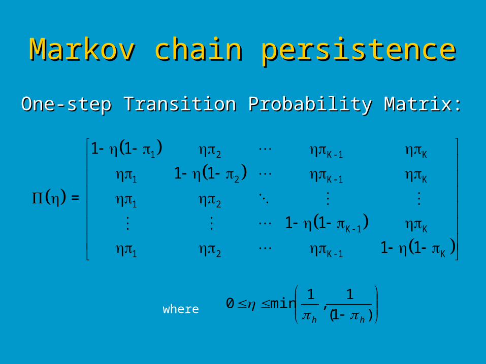
One-step transition probabilities:One-step transition probabilities:
LikelihoodLikelihood
hpr h)habitat tomove(
)1(1h)habitat in stay ( hpr
F
i
H
h
vh
vh
f
h
ihhihhihP1 1
)))1((1()(),|( * πX
= number of moves from habitat h* to habitat h ;
*ihhv
ihf = indicator for initial sighting habitat= number of stays in habitat h ;ihhv

Bayesian extensions
I.I. Reformulation of the original non-seasonal Reformulation of the original non-seasonal persistence model into Bayesian framework:persistence model into Bayesian framework:
II.II. Non-seasonal persistence / Seasonal HSPs:Non-seasonal persistence / Seasonal HSPs:
III.III. Seasonal persistence / Non-seasonal HSPs:Seasonal persistence / Non-seasonal HSPs:
IV.IV. Seasonal persistence / Seasonal HSPs:Seasonal persistence / Seasonal HSPs:
),( sh
),( shs
),( hs
),( h

II. Non-seasonal persistence/Seasonal HSPsII. Non-seasonal persistence/Seasonal HSPs
LikelihoodLikelihood
),( sh
F
i
S
s
H
h
vsh
vsh
vf
sh
ihhihhnsihhihP1 1 1
)))1((1(),|( **, πX
sh
shsh
sh
= habitat selection probability for habitat h in season ssh = overall persistence parameter

Multinomial logit Multinomial logit parameterizationparameterization
Habitat Selection Probability (HSP):Habitat Selection Probability (HSP):
Multinomial logit parameterization:Multinomial logit parameterization:
sh
shsh
shhTR
shsh
)Aratln(ln)logit(
TR
sh
Area
AreaArat
s = 1, …, S h = 1, …, H i = 1, …, F
T = reference seasonR = reference habitat
0 sRThR
sh
sh

IIIIII.. Seasonal persistence / Non-seasonal HSPsSeasonal persistence / Non-seasonal HSPs
F
i
S
s
H
h
vhs
vhs
f
h
ishhishhishP1 1 1
)))1((1()(),|( * ηπX
h h
hh
LikelihoodLikelihood
),( hs
ishf = indicator for initial sighting habitat h in season s
= number of stays in habitat h in season sishhv= number of moves from habitat h* to habitat h in season s*ishhv
IV. Seasonal persistence / Seasonal HSPsIV. Seasonal persistence / Seasonal HSPs),( shs
F
i
S
s
H
h
vshs
vshs
f
sh
ishhishhishP1 1 1
)))1((1()(),|( * ηπX
sh sh
shsh
LikelihoodLikelihood
Priors for all modelsPriors for all models
h ~ diffuse normal
sh ~ diffuse normal
),0( I
),0( Is
ss
ss

ROBERTS Persistence Parameter (eta): 95% Posterior Intervals
persistence parameter
0.0 0.2 0.4 0.6 0.8 1.0
Non-seasonal persistence / Seasonal HSP model
( )
Seasonal persistence / Non-seasonal HSP model
( )WINTER
( )SPRING
( )SUMMER
Seasonal persistence / Seasonal HSP model
( )WINTER
( )SPRING
( )SUMMER
Estimated persistence parameters:Estimated persistence parameters:Roberts CreekRoberts Creek
s
ss
s
),( sh
),( shs
),( hs

RAIL Persistence Parameter (eta): 95% Posterior Intervals
persistence parameter
0.0 0.2 0.4 0.6 0.8 1.0
Non-seasonal persistence / Seasonal HSP model
( )
Seasonal persistence / Non-seasonal HSP model
( )WINTER
( )SPRING
( )SUMMER
Seasonal persistence / Seasonal HSP model
( )WINTER
( )SPRING
( )SUMMER
Estimated persistence parameters:Estimated persistence parameters:Rail CreekRail Creek
s
ss
s
),( sh
),( shs
),( hs
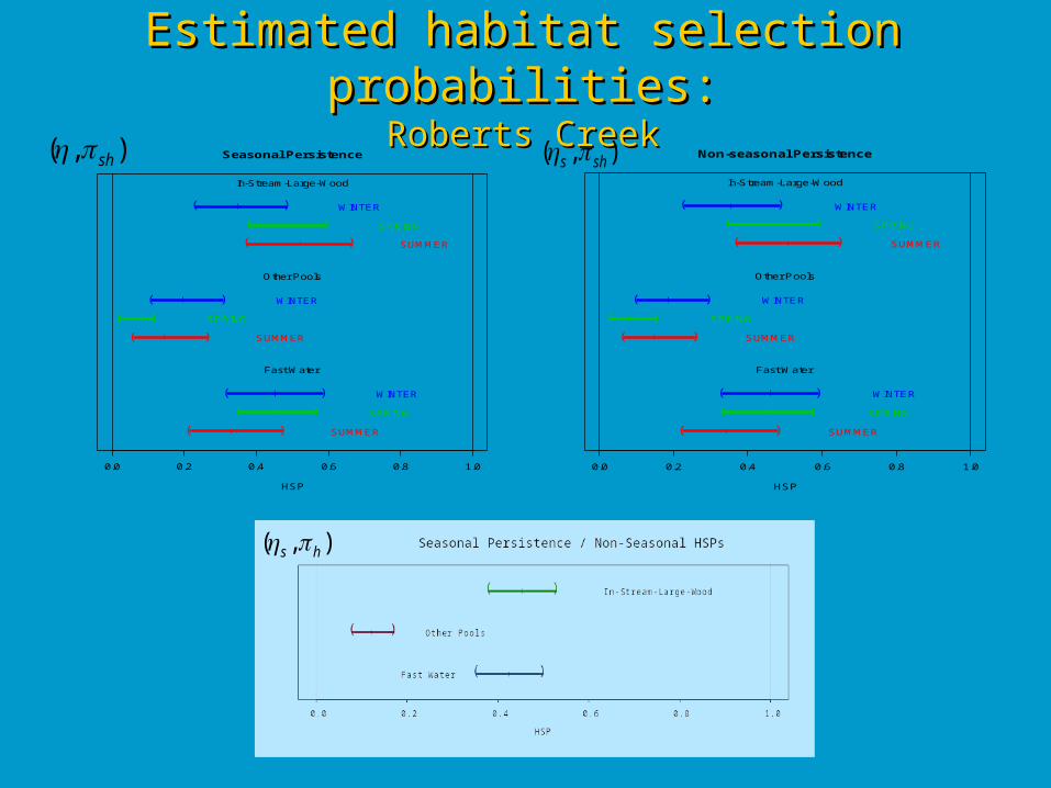
Estimated habitat selection probabilities:Estimated habitat selection probabilities:Roberts CreekRoberts Creek
0.0 0.2 0.4 0.6 0.8 1.0
Non-seasonal Persistence
HSP
In-Stream-Large-Wood
( ) WINTER
( ) SPRING
( ) SUMMER
Other Pools
( ) WINTER
( ) SPRING
( ) SUMMER
Fast Water
( ) WINTER
( ) SPRING
( ) SUMMER
0.0 0.2 0.4 0.6 0.8 1.0
Seasonal Persistence
HSP
In-Stream-Large-Wood
( ) WINTER
( ) SPRING
( ) SUMMER
Other Pools
( ) WINTER
( ) SPRING
( ) SUMMER
Fast Water
( ) WINTER
( ) SPRING
( ) SUMMER
),( shs
),( hs
),( sh

Non-seasonal Persistence
SPR/AR
0 10 20 30 40 50
In-Stream-Large-Wood
( ) WINTER
( ) SPRING
( ) SUMMER
Other Pools
( ) WINTER
( ) SPRING
( ) SUMMER
Fast Water
WINTER
SPRING
SUMMER
Seasonal Persistence
SPR/AR
0 10 20 30 40 50
In-Stream-Large-Wood
( ) WINTER
( ) SPRING
( ) SUMMER
Other Pools
( ) WINTER
( ) SPRING
( ) SUMMER
Fast Water
WINTER
SPRING
SUMMER
Selection Probability Ratio/Area Ratio:Selection Probability Ratio/Area Ratio:Rail CreekRail Creek
s
ss
s
),( sh ),( shs

BIC comparisonBIC comparison
MODELMODEL PersistencePersistence HSPHSP BIC RobertsBIC Roberts BIC RailBIC Rail
II NS NS 742.6 482.2482.2
IIII NS seasonal 751.2 479.4479.4
IIIIII seasonal NS 711.6 ** 467.8 **467.8 **
IVIV seasonal seasonal 717.0 469.2469.2
),( sh ),( shs ),( hs
BIC = -2*log(likelihood) + p*log(n)
),( h
ConclusionsConclusions Relaxes assumption of independent sightingsRelaxes assumption of independent sightings
Biological meaningfulness of the persistence parameterBiological meaningfulness of the persistence parameter
Provides a single model for the estimation of seasonal Provides a single model for the estimation of seasonal persistence parameters and other estimates of interest persistence parameters and other estimates of interest (HSP, (SPR/Arat)), along with their respective uncertainty (HSP, (SPR/Arat)), along with their respective uncertainty intervalsintervals
Allows for seasonal comparisons and the incorporation of Allows for seasonal comparisons and the incorporation of multiple study areas (streams)multiple study areas (streams)
Allows for use of other covariates by changing the Allows for use of other covariates by changing the parameterization of the multinomial logitparameterization of the multinomial logit

THANK YOUTHANK YOUs
sh
sh
sh
sh
sh
shs
s
s
s
s
s s
s
s
ss s

V.V. Multiple stream persistence Multiple stream persistence
C
c
F
i
S
s
H
h
vcshcs
vcshcs
f
csh
icshhicshhicshP1 1 1 1
)))1((1()(),|( * ηπX
LikelihoodLikelihood
icshf = indicator for initial sighting in habitat h in season s in stream c
= number of stays in habitat h in season s in stream cicshhv
= number of moves from habitat h* to habitat h in season s in stream c
*icshhv
),( cshcs

Evidence of persistenceEvidence of persistenceRoberts CreekRoberts Creek
05
01
00
15
02
00
Number of persists and moves per season
Winter Spring Summer
PersistsMoves
Winter Spring Summer
0.0
0.2
0.4
0.6
0.8
1.0
Percent persists of total sightings
Markov chain persistenceMarkov chain persistence
One-step Transition Probability Matrix:One-step Transition Probability Matrix:
1 2 K 1 K
1 2 K 1 K
1 2
K 1 K
1 2 K 1 K
1 1
1 1
=
1 1
1 1
)1(
1,
1min0
hh where

Persistence examplePersistence example
= 1 1 2 3
1 0.2 0.3 0.5
2 0.2 0.3 0.5
3 0.2 0.3 0.5
= 0.5 1 2 3
1 0.60 0.15 .25
2 0.10 0.65 .25
3 0.10 0.15 0.75
= 1 -> IMS= 1 -> IMS < 1 -> greater chance of remaining in previous habitat< 1 -> greater chance of remaining in previous habitat

Estimate of Use vs. availabilityEstimate of Use vs. availability Selection Probability Ratio (SPR)Selection Probability Ratio (SPR)
SPR/(Area Ratio) for Use vs. AvailabilitySPR/(Area Ratio) for Use vs. Availability
shhTR
sh SPR
Arat)ln()ln(ln
Arat
SPR
)exp( shhArat
SPR
)exp(Arat shhTR
shSPR
Arat
SPRArat
SPR
Arat
SPR

Persistence vs. IMSPersistence vs. IMS
Persistence vs. IMS: SPR/AreaRatio Wald's 95% CIs
SPR/AR
0 5 10 15 20
( ) Winter RIFFLE-PERS( ) Winter RIFFLE-IMS
( ) Winter GLIDE-PERS( )
Winter GLIDE-IMS( ) Winter SCOUR-PERS
( )Winter SCOUR-IMS
() Spring RIFFLE-PERS() Spring RIFFLE-IMS
( ) Spring GLIDE-PERS( ) Spring GLIDE-IMS
( ) Spring SCOUR-PERS( ) Spring GLIDE-IMS

Estimated persistence parametersEstimated persistence parameters
0.0 0.2 0.4 0.6 0.8 1.0
ROBERTS Persistence Parameter (eta): 95% Posterior Intervals
Eta
Hierarchical seasonal model
( )WINTER
( )SPRING
( )SUMMER
( )OVERALL Persistence
Non-seasonal persistence, seasonal HSPs model
( ) persistence parameter

stuffstuff
BIC = -2*mean(llik[1001:10000]) - p*log(17)
model IV. p = 7 in basemodelROB and
model III. p = 5 in seaspersonlyROB

PriorsPriors
Multinomial logit parameters:Multinomial logit parameters:
Non-seasonal persistence:Non-seasonal persistence:
Seasonal persistence:Seasonal persistence:
Hierarchical seasonal persistence:Hierarchical seasonal persistence:
h ~ diffuse normal
sh ~ diffuse normal
s )1,0(Unif~
)1,0(Unif~
s ~ Beta(a,b) a,b ),0(Unif~
Top Related