
Languages
Pages
Legal


Automated Tracking of Whiskers in Videos of Head FixedRodentsNathan G. Clack*, Daniel H. O’Connor, Daniel Huber, Leopoldo Petreanu, Andrew Hires, Simon Peron,
Karel Svoboda, Eugene W. Myers
Janelia Farm Research Campus, Howard Hughes Medical Institute, Ashburn, Virginia, United States of America
Abstract
We have developed software for fully automated tracking of vibrissae (whiskers) in high-speed videos (.500 Hz) of head-fixed, behaving rodents trimmed to a single row of whiskers. Performance was assessed against a manually curated datasetconsisting of 1.32 million video frames comprising 4.5 million whisker traces. The current implementation detects whiskerswith a recall of 99.998% and identifies individual whiskers with 99.997% accuracy. The average processing rate for theseimages was 8 Mpx/s/cpu (2.6 GHz Intel Core2, 2 GB RAM). This translates to 35 processed frames per second for a640 px6352 px video of 4 whiskers. The speed and accuracy achieved enables quantitative behavioral studies where theanalysis of millions of video frames is required. We used the software to analyze the evolving whisking strategies as micelearned a whisker-based detection task over the course of 6 days (8148 trials, 25 million frames) and measure the forces atthe sensory follicle that most underlie haptic perception.
Citation: Clack NG, O’Connor DH, Huber D, Petreanu L, Hires A, et al. (2012) Automated Tracking of Whiskers in Videos of Head Fixed Rodents. PLoS ComputBiol 8(7): e1002591. doi:10.1371/journal.pcbi.1002591
Editor: Andreas Prlic, University of California, San Diego, United States of America
Received January 23, 2012; Accepted May 12, 2012; Published July 5, 2012
Copyright: � 2012 Clack et al. This is an open-access article distributed under the terms of the Creative Commons Attribution License, which permitsunrestricted use, distribution, and reproduction in any medium, provided the original author and source are credited.
Funding: The Howard Hughes Medical Institute funded this work (www.hhmi.org). The funders had no role in study design, data collection and analysis, decisionto publish, or preparation of the manuscript.
Competing Interests: The authors have declared that no competing interests exist.
* E-mail: [email protected]
‘‘This is a PLoS Computational Biology Software article.’’
Introduction
Rats and mice move their large whiskers (vibrissae), typically in
a rhythmic pattern, to locate object features [1,2], or to identify
textures and objects [3,4]. Whisker movements in turn are
influenced by touch [1,5]. The whisker system is a powerful
model for studying the principles underlying sensorimotor
integration and active somatosensation [6]. Critical to any
mechanistic study at the level of neurons is the quantitative
analysis of behavior. Whisker movements have been measured in a
variety of ways. Electromyograms, recorded from the facial
muscles, correlate with whisker movements [7]. This invasive
method does not report whisker position and shape per se and is
complimentary to whisker tracking. Imaging individual labeled
whiskers, for example by gluing a high-contrast particle on the
whisker [8], provides the position of the marked whisker, but does
not reveal whisker shape. In addition, the particle will change the
whisker mass and stiffness and thereby perturb whisker dynamics.
Monitoring a single point along the whisker using linescan imaging
[9], or a linear light sheet [10], can provide high-speed
information about whisker position, but only at a single line of
intersection.
High-speed (.500 Hz) videography is a non-invasive method
for measuring whisker movements and forces acting on whiskers
and yields nearly complete information about whiskers during
behavior [1,11–15]. The position of the whisker base with respect
to the face reveals the motor programs underlying behavior. The
deformation of whisker shape by touch can be used to extract the
forces felt by the mouse sensory follicles [16,17]. However, high-
speed videography brings its own technical challenges. The large
number of images required makes manual analysis impossible for
more than a few seconds of video. Comprehensive studies require
fully automated analysis. In addition, extraction of motions and
touch forces demands accurate measurement of whisker shape,
often with sub-pixel precision, and identification of rapidly moving
whiskers across time. Finally, the large volume of video data
potentially places severe demands even on advanced computa-
tional infrastructures, making efficient algorithms necessary.
Tracking whiskers is challenging. Whiskers can move at high
speeds [12] and in complex patterns [1,18]. Adjacent whiskers can
have distinct trajectories. Moreover, whiskers are thin hairs (e.g.
mouse whiskers taper to a thickness of a few micrometers) and thus
provide only limited contrast in imaging experiments.
To address these challenges, we have developed software for
tracking a single row of whiskers in a fully automated fashion.
Over a manually curated database of 400 video sequences of head
fixed mice (1.326106 cumulative images, 4.56106 traced whiskers,
8 mice), whiskers were correctly detected and identified with an
accuracy of 99.997% (1 error per 36104 traced whiskers). In other
whisker tracking systems, models constraining possible motions
and whisker shapes have been used to aid tracking. In contrast, our
approach uses statistics gleaned from the video itself to estimate
the most likely identity of each traced object that maintains the
expected order of whiskers along the face. As a result, the shapes of
highly strained whiskers (curvature.0.25/mm) can be traced with
sub-pixel accuracy, and tracking is faithful despite occasional fast
motion (deflections .10,000 degrees/s).
PLoS Computational Biology | www.ploscompbiol.org 1 July 2012 | Volume 8 | Issue 7 | e1002591
Our method consists of two steps performed in succession:
tracing and linking. Tracing produces a set of piecewise linear
curves that represent whisker-like objects for each individual image
in a video. Each image is analyzed independently. The linking
algorithm is then applied to determine the identity of each traced
curve. The trajectory of a whisker is described by collecting curves
with the same identity throughout the video. Importantly, once a
faithful tracing is completed, the original voluminous image data
set is no longer required for downstream processing.
Once tracing is complete, a small set of features is tabulated for
each curve. Based on these features, a heuristic is used to make an
initial guess as to the identity of curves in a set of images where it
works well. These initial identifications are then used to get a
statistical description of the shapes and motions of whiskers. These
statistics are then used to compute a final optimal labeling for each
traced curve subject to the constraint that whiskers are ordered
along the face.
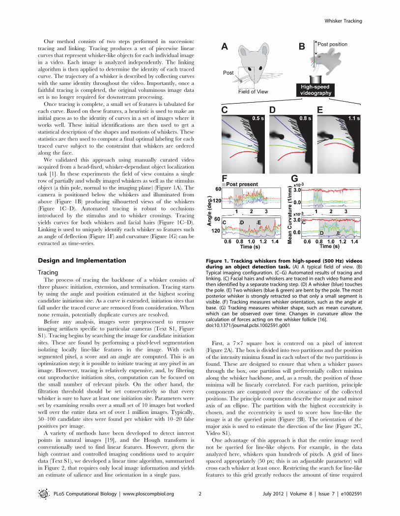
We validated this approach using manually curated video
acquired from a head-fixed, whisker-dependant object localization
task [1]. In these experiments the field of view contains a single
row of partially and wholly imaged whiskers as well as the stimulus
object (a thin pole, normal to the imaging plane) (Figure 1A). The
camera is positioned below the whiskers and illuminated from
above (Figure 1B) producing silhouetted views of the whiskers
(Figure 1C–D). Automated tracing is robust to occlusions
introduced by the stimulus and to whisker crossings. Tracing
yields curves for both whiskers and facial hairs (Figure 1C–D).
Linking is used to uniquely identify each whisker so features such
as angle of deflection (Figure 1F) and curvature (Figure 1G) can be
extracted as time-series.
Design and Implementation
TracingThe process of tracing the backbone of a whisker consists of
three phases: initiation, extension, and termination. Tracing starts
by using the angle and position estimated at the highest scoring
candidate initiation site. As a curve is extended, initiation sites that
fall under the traced curve are removed from consideration. When
none remain, potentially duplicate curves are resolved.
Before any analysis, images were preprocessed to remove
imaging artifacts specific to particular cameras (Text S1, Figure
S1). Tracing begins by searching the image for candidate initiation
sites. These are found by performing a pixel-level segmentation
isolating locally line-like features in the image. With each
segmented pixel, a score and an angle are computed. This is an
optimization step; it is possible to initiate tracing at any pixel in an
image. However, tracing is relatively expensive, and, by filtering
out unproductive initiation sites, computation can be focused on
the small number of relevant pixels. On the other hand, the
filtration threshold should be set conservatively so that every
whisker is sure to have at least one initiation site. Parameters were
set by examining results over a small set of 10 images but worked
well over the entire data set of over 1 million images. Typically,
50–100 candidate sites were found per whisker with 10–20 false
positives per image.
A variety of methods have been developed to detect interest
points in natural images [19], and the Hough transform is
conventionally used to find linear features. However, given the
high contrast and controlled imaging conditions used to acquire
data (Text S1), we developed a linear time algorithm, summarized
in Figure 2, that requires only local image information and yields
an estimate of salience and line orientation in a single pass.
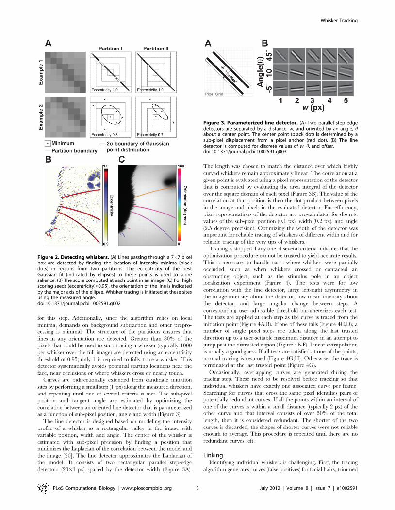
First, a 767 square box is centered on a pixel of interest
(Figure 2A). The box is divided into two partitions and the position
of the intensity minima found in each subset of the two partitions is
found. These are designed to ensure that when a whisker passes
through the box, one partition will preferentially collect minima
along the whisker backbone, and, as a result, the position of those
minima will be linearly correlated. For each partition, principle
components are computed over the covariance of the collected
positions. The principle components describe the major and minor
axis of an ellipse. The partition with the highest eccentricity is
chosen, and the eccentricity is used to score how line-like the
image is at the queried point (Figure 2B). The orientation of the
major axis is used to estimate the direction of the line (Figure 2C,
Video S1).
One advantage of this approach is that the entire image need
not be queried for line-like objects. For example, in the data
analyzed here, whiskers span hundreds of pixels. A grid of lines
spaced appropriately (50 px; this is an adjustable parameter) will
cross each whisker at least once. Restricting the search for line-like
features to this grid greatly reduces the amount of time required
Figure 1. Tracking whiskers from high-speed (500 Hz) videosduring an object detection task. (A) A typical field of view. (B)Typical imaging configuration. (C–G) Automated results of tracing andlinking. (C) Facial hairs and whiskers are traced in each video frame andthen identified by a separate tracking step. (D) A whisker (blue) touchesthe pole. (E) Two whiskers (blue & green) are bent by the pole. The mostposterior whisker is strongly retracted so that only a small segment isvisible. (F) Tracking measures whisker orientation, such as the angle atbase. (G) Tracking measures whisker shape, such as mean curvature,which can be observed over time. Changes in curvature allow thecalculation of forces acting on the whisker follicle [16].doi:10.1371/journal.pcbi.1002591.g001
Whisker Tracking
PLoS Computational Biology | www.ploscompbiol.org 2 July 2012 | Volume 8 | Issue 7 | e1002591
for this step. Additionally, since the algorithm relies on local
minima, demands on background subtraction and other prepro-
cessing is minimal. The structure of the partitions ensures that
lines in any orientation are detected. Greater than 80% of the
pixels that could be used to start tracing a whisker (typically 1000
per whisker over the full image) are detected using an eccentricity
threshold of 0.95; only 1 is required to fully trace a whisker. This
detector systematically avoids potential starting locations near the
face, near occlusions or where whiskers cross or nearly touch.
Curves are bidirectionally extended from candidate initiation
sites by performing a small step (1 px) along the measured direction,
and repeating until one of several criteria is met. The sub-pixel
position and tangent angle are estimated by optimizing the
correlation between an oriented line detector that is parameterized
as a function of sub-pixel position, angle and width (Figure 3).
The line detector is designed based on modeling the intensity
profile of a whisker as a rectangular valley in the image with
variable position, width and angle. The center of the whisker is
estimated with sub-pixel precision by finding a position that
minimizes the Laplacian of the correlation between the model and
the image [20]. The line detector approximates the Laplacian of
the model. It consists of two rectangular parallel step-edge
detectors (2061 px) spaced by the detector width (Figure 3A).
The length was chosen to match the distance over which highly
curved whiskers remain approximately linear. The correlation at a
given point is evaluated using a pixel representation of the detector
that is computed by evaluating the area integral of the detector
over the square domain of each pixel (Figure 3B). The value of the
correlation at that position is then the dot product between pixels
in the image and pixels in the evaluated detector. For efficiency,
pixel representations of the detector are pre-tabulated for discrete
values of the sub-pixel position (0.1 px), width (0.2 px), and angle
(2.5 degree precision). Optimizing the width of the detector was
important for reliable tracing of whiskers of different width and for
reliable tracing of the very tips of whiskers.
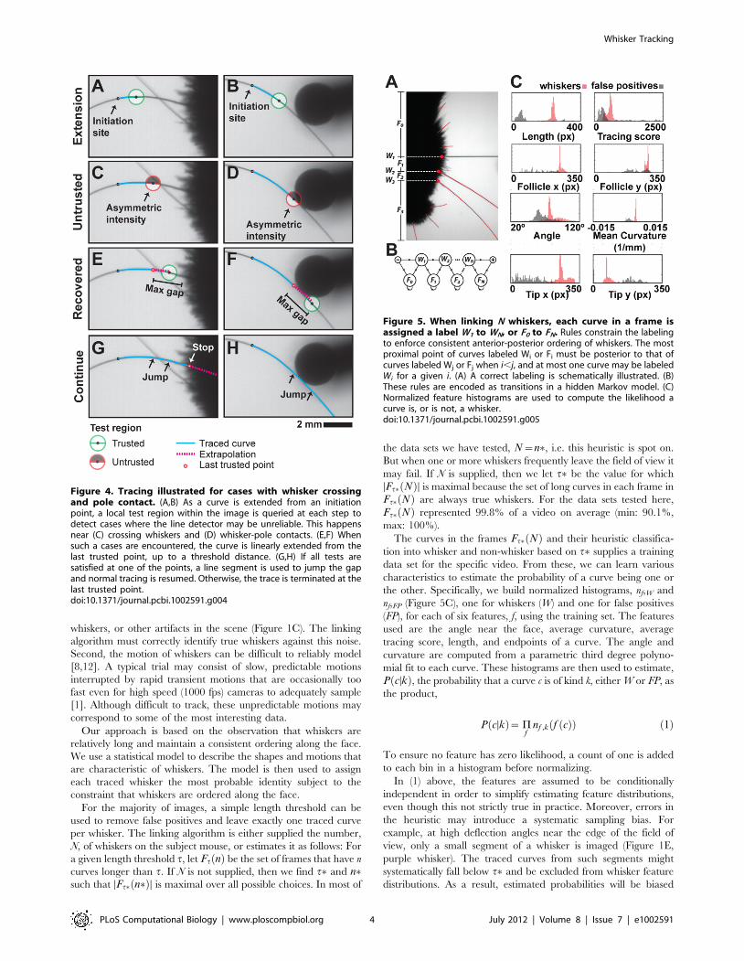
Tracing is stopped if any one of several criteria indicates that the
optimization procedure cannot be trusted to yield accurate results.
This is necessary to handle cases where whiskers were partially
occluded, such as when whiskers crossed or contacted an
obstructing object, such as the stimulus pole in an object
localization experiment (Figure 4). The tests were for low
correlation with the line detector, large left-right asymmetry in
the image intensity about the detector, low mean intensity about
the detector, and large angular change between steps. A
corresponding user-adjustable threshold parameterizes each test.
The tests are applied at each step as the curve is traced from the
initiation point (Figure 4A,B). If one of these fails (Figure 4C,D), a
number of single pixel steps are taken along the last trusted
direction up to a user-settable maximum distance in an attempt to
jump past the distrusted region (Figure 4E,F). Linear extrapolation
is usually a good guess. If all tests are satisfied at one of the points,
normal tracing is resumed (Figure 4G,H). Otherwise, the trace is
terminated at the last trusted point (Figure 4G).
Occasionally, overlapping curves are generated during the
tracing step. These need to be resolved before tracking so that
individual whiskers have exactly one associated curve per frame.
Searching for curves that cross the same pixel identifies pairs of
potentially redundant curves. If all the points within an interval of
one of the curves is within a small distance (typically 2 px) of the
other curve and that interval consists of over 50% of the total
length, then it is considered redundant. The shorter of the two
curves is discarded; the shapes of shorter curves were not reliable
enough to average. This procedure is repeated until there are no
redundant curves left.
LinkingIdentifying individual whiskers is challenging. First, the tracing
algorithm generates curves (false positives) for facial hairs, trimmed
Figure 2. Detecting whiskers. (A) Lines passing through a 767 pixelbox are detected by finding the location of intensity minima (blackdots) in regions from two partitions. The eccentricity of the bestGaussian fit (indicated by ellipses) to these points is used to scoresalience. (B) The score computed at each point in an image. (C) For highscoring seeds (eccentricity.0.95), the orientation of the line is indicatedby the major axis of the ellipse. Whisker tracing is initiated at these sitesusing the measured angle.doi:10.1371/journal.pcbi.1002591.g002
Figure 3. Parameterized line detector. (A) Two parallel step edgedetectors are separated by a distance, w, and oriented by an angle, habout a center point. The center point (black dot) is determined by asub-pixel displacement from a pixel anchor (red dot). (B) The linedetector is computed for discrete values of w, h, and offset.doi:10.1371/journal.pcbi.1002591.g003
Whisker Tracking
PLoS Computational Biology | www.ploscompbiol.org 3 July 2012 | Volume 8 | Issue 7 | e1002591
whiskers, or other artifacts in the scene (Figure 1C). The linking
algorithm must correctly identify true whiskers against this noise.
Second, the motion of whiskers can be difficult to reliably model
[8,12]. A typical trial may consist of slow, predictable motions
interrupted by rapid transient motions that are occasionally too
fast even for high speed (1000 fps) cameras to adequately sample
[1]. Although difficult to track, these unpredictable motions may
correspond to some of the most interesting data.
Our approach is based on the observation that whiskers are
relatively long and maintain a consistent ordering along the face.
We use a statistical model to describe the shapes and motions that
are characteristic of whiskers. The model is then used to assign
each traced whisker the most probable identity subject to the
constraint that whiskers are ordered along the face.
For the majority of images, a simple length threshold can be
used to remove false positives and leave exactly one traced curve
per whisker. The linking algorithm is either supplied the number,
N, of whiskers on the subject mouse, or estimates it as follows: For
a given length threshold t, let Ft nð Þ be the set of frames that have n
curves longer than t. If N is not supplied, then we find t� and n�such that DFt� n�ð ÞD is maximal over all possible choices. In most of
the data sets we have tested, N~n�, i.e. this heuristic is spot on.
But when one or more whiskers frequently leave the field of view it
may fail. If N is supplied, then we let t� be the value for which
DFt� Nð ÞD is maximal because the set of long curves in each frame in
Ft� Nð Þ are always true whiskers. For the data sets tested here,
Ft� Nð Þ represented 99.8% of a video on average (min: 90.1%,
max: 100%).
The curves in the frames Ft� Nð Þ and their heuristic classifica-
tion into whisker and non-whisker based on t� supplies a training
data set for the specific video. From these, we can learn various
characteristics to estimate the probability of a curve being one or
the other. Specifically, we build normalized histograms, nf,W and
nf,FP (Figure 5C), one for whiskers (W) and one for false positives
(FP), for each of six features, f, using the training set. The features
used are the angle near the face, average curvature, average
tracing score, length, and endpoints of a curve. The angle and
curvature are computed from a parametric third degree polyno-
mial fit to each curve. These histograms are then used to estimate,
P cDkð Þ, the probability that a curve c is of kind k, either W or FP, as
the product,
P cDkð Þ~Pf
nf ,k f cð Þð Þ ð1Þ
To ensure no feature has zero likelihood, a count of one is added
to each bin in a histogram before normalizing.
In (1) above, the features are assumed to be conditionally
independent in order to simplify estimating feature distributions,
even though this not strictly true in practice. Moreover, errors in
the heuristic may introduce a systematic sampling bias. For
example, at high deflection angles near the edge of the field of
view, only a small segment of a whisker is imaged (Figure 1E,
purple whisker). The traced curves from such segments might
systematically fall below t� and be excluded from whisker feature
distributions. As a result, estimated probabilities will be biased
Figure 4. Tracing illustrated for cases with whisker crossingand pole contact. (A,B) As a curve is extended from an initiationpoint, a local test region within the image is queried at each step todetect cases where the line detector may be unreliable. This happensnear (C) crossing whiskers and (D) whisker-pole contacts. (E,F) Whensuch a cases are encountered, the curve is linearly extended from thelast trusted point, up to a threshold distance. (G,H) If all tests aresatisfied at one of the points, a line segment is used to jump the gapand normal tracing is resumed. Otherwise, the trace is terminated at thelast trusted point.doi:10.1371/journal.pcbi.1002591.g004
Figure 5. When linking N whiskers, each curve in a frame isassigned a label W1 to WN, or F0 to FN. Rules constrain the labelingto enforce consistent anterior-posterior ordering of whiskers. The mostproximal point of curves labeled Wi or Fi must be posterior to that ofcurves labeled Wj or Fj when i,j, and at most one curve may be labeledWi for a given i. (A) A correct labeling is schematically illustrated. (B)These rules are encoded as transitions in a hidden Markov model. (C)Normalized feature histograms are used to compute the likelihood acurve is, or is not, a whisker.doi:10.1371/journal.pcbi.1002591.g005
Whisker Tracking
PLoS Computational Biology | www.ploscompbiol.org 4 July 2012 | Volume 8 | Issue 7 | e1002591

towards longer whiskers at milder deflection angles. Despite these
caveats, the use of these feature distributions leads to a highly
accurate result.
Appearance alone is not sufficient to uniquely identify
individual whiskers in some cases. To address this, we designed
a naive Bayes’ classifier to determine the most probable identity of
each traced curve subject to ordering constraints. The traced
curves are ordered into a sequence, C, according to their time and
relative anterior-posterior position. Identifying a curve, c, involves
assigning a particular label, l, from the following set of 2N+1 labels.
There is a label for each whisker, W1 to WN, and labels, F0 to FN,
where Fi identifies all false positives between whisker Wi and Wi+1
(Figure 5A). The kind of a label, K(l), is W if l is a whisker label,
and FP if l is a false positive label. A curve labeled Wi or Fi must be
posterior to curves labeled Wj or Fj for all i,j. For a given i, only
one curve per frame may be labeled Wi, but several curves may be
labeled Fi.
Applying Bayes’ theorem, the most probable sequence of labels,
L̂L, is given by
L̂L~ arg maxL
P Lð ÞP CDLð Þ ð2Þ
where P Lð Þ is the a priori probability of a labeling sequence, and
P CDLð Þ is the likelihood that the curves in C are generated from
the sequence of items labeled by L. By design, certain labeling
sequences are ruled out a priori. Conceptually drawing a directed
edge between one identity and the possible identities of the next
curve yields a directed graph (Figure 5B). For a video with T
frames,
P Lð Þ~ PT
t~1P lt
1
� �PNt
i~2P lt
i Dlti{1
� � !ð3Þ
where N t is the number of curves traced in frame t, and lti is the
label of the i’th curve found in frame t. Values for P lt1
� �and
P lti Dl
ti{1
� �are estimated by computing the frequency of observed
label pairs that occur in the a training set, Ft� Nð Þ. This describes a
hidden Markov model for labeling curves in a single video frame.
The optimal labeling can be computed efficiently with well-known
dynamic programming techniques [21].
The likelihood, P CDLð Þ, is computed under the simplifying
assumption that the likelihood of a single curve depends only on
the curves in the previous or following frame. Using this and
applying Bayes’ theorem,
P CDLð Þ! PT
t~1P
c[CtP cDK lcð Þð ÞP cDCt+1,Lt+1,lc
� �ð4Þ
where lc is the label L assigns to the curve c, C t is the (possibly
empty) set of curves found in frame t, and Lt are the labels
assigned to the curves in Ct. The first component, P cDK lcð Þð Þ, is
the likelihood that c is an object of the kind denoted by label l
which we estimate with formula (1).
The second component of (4), P cDCt+1,Lt+1,l� �
, is interpreted
as the likelihood that a curve is part of the same trajectory as
corresponding curves in the previous (or following) frame. Similar
to the approach used in equation (1) for estimating P cDkð Þ, we
need normalized histograms nDf ,W and nDf ,FP of the changes of
whiskers and false positives between successive frames for each
feature f over a ‘‘training’’ data set in which the corresponding
curves in successive frames is known. While we could use the
implied assignment over Ft� Nð Þ, we first estimate a hopefully
better assignment by restricting the model in (4) to use shape
features alone. That is, P cDCt+1,Lt+1,l� �
is treated as a constant
and thus the assignment to labels in a frame can be computed
independently of other frames. We then use this preliminary
labeling over the frames of Ft� Nð Þ as the training set over which to
build nDf ,W and nDf ,FP.
Given these change histograms, one can estimate the corre-
spondence likelihood according to the formula,
P c Ct+1,Lt+1,l��� �
~
Pf
nDf ,K(l) f cð Þ{f bð Þð Þ K(l)~W and Ab[Ct+1 s:t: lb~l
maxb[Ct{1
Pf
nDf ,K(l) f cð Þ{f bð Þð Þ otherwise
8><>:
ð5Þ
Note that when evaluating this likelihood, a unique corresponding
curve is not always present in the previous (or following) frame.
There may be zero or many false positive curves in the previous
frame with the same label. Similarly a whisker may be missing
because it exited the field of view.
Directly solving for the most probable labeling (2) is complicated
by the fact that the likelihood of a labeling in one frame depends
on the labeling in neighboring frames. Our approach is to initially
score each frame by computing P L̂LtDCt� �
~P L̂Lt� �
P CtDL̂Lt� �
,
where L̂L is obtained using shape features alone. In decreasing
order of this score, we ‘visit’ the next best frame, say t, and update
the label assignment for each of the two adjacent frames that
maximizes the full version of (4), provided the adjacent frame has
not already been visited. The new assignment replaces the current
assignment and the frame’s visitation order is updated according
to the score of this new assignment (under the full model of (4)). In
this way, we let the most confident frames influence their
neighbors in a transitive fashion until every frame has been
visited. This was critical for achieving high accuracy. Previous
whisker tracking algorithms have relied on propagating the
identity of a whisker frame-wise from the beginning of the video
to the end, and as a result, an error in one frame is propagated
throughout the rest of the video [11–13].
Results/Discussion
Average processing time was 8 Mpx/s/cpu (35 fps for 6406352
pixel video) measured on a 2.6 GHz Intel Core2 Duo Macbook
Pro with 2 GB of RAM, and was dominated by the CPU time
required to trace curves; linking time was 0.5 ms per frame. This is
faster than published speeds of similar whisker analysis packages
(typically, 1–5 fps.) [11,13,15]. However, performance can be
difficult to compare as implementations may improve over time.
For example, our software is equally fast as the current version of
the only other publically available whisker tracker[13]. More
importantly, our software can readily be run on inexpensive cluster
nodes to process videos in parallel. This is not the case for whisker
trackers that require supervision [13] or that depend on software
with expensive licensing requirements (such as Matlab) [11–15].
Tracing was accurate to within 0.2 px as estimated by analyzing
39 hand-traced whiskers. Individual hand-tracings had an
accuracy of 0.2360.2 pixels when compared against consensus
curves. Mouse whiskers (row C) were automatically traced in
images with resolutions from 5 mm/px to 320 mm/px using default
settings and in noisy, low-contrast images (Text S1). For the best
results, it is important to minimize motion blur and uniformly
illuminate the scene, although illumination inhomogeneities can
Whisker Tracking
PLoS Computational Biology | www.ploscompbiol.org 5 July 2012 | Volume 8 | Issue 7 | e1002591

be partially corrected with background subtraction. In contrast
with methods that use Kalman filtering [13], traced curves are not
biased by whisker dynamics. Additionally, tracing is faithful even
when curves are not well approximated by low order polynomials,
in contrast to published tracing methods [13–15]. Whiskers could
be detected and traced in videos of freely behaving rats (Video S2)
and mice (Video S3) with all whiskers intact.
Linking accuracy was measured against a hand-annotated set of
videos selected by choosing 100 random trials from behavioral
sessions of 4 mice (1.32 million frames) [1,17]. The curated videos
captured a range of behavior including protracted bouts (.1 s) of
whisking (Video S4), multiple whiskers simultaneously contacting
an object (a thin metal pole) (Video S4), and extremely fast motion
(.10,000u/second) (Video S5). Of the 4.5 million traced whiskers,
130 were incorrectly identified or not detected, less than one
mistake per behavioral trial on average. Linking is robust to
whiskers that occasionally leave the field of view (Video S6), and
works well even at relatively low frame rates (100 fps; see Text S1).
Lesser image quality will ultimately degrade results.
There are two principle sources of error in the linking. First,
covariance between different features is ignored. For example,
when the field of view is small, whiskers at high deflection angles
might not be fully contained within the image. Any curve tracing
one of these whiskers would appear shorter than the full whisker
length. Under these conditions there is a strong correlation
between angle and whisker length. The current model penalizes
the shorter length because it is rarely observed; accounting for the
covariance should eliminate this problem. Second, the estimated
feature distributions are affected by systematic biases introduced
from the heuristic used to initially guess whisker identity. A
heuristic relying on a length threshold, like the one used here, may
systematically reject these short curves at high deflection angle.
This will result in a bias against strongly deflected whiskers.
Fundamentally, our linking method is applicable only to single
rows of whiskers. The whiskers in videos imaging multiple rows of
whiskers will be traced, but, because whisker images no longer
maintain a strict anterior-posterior ordering, the linking will likely
fail. Although this software was validated with images of one side
of the mouse’s whiskers, we have successfully tracked whiskers in
images containing both whisker fields (Video S7). Also, the
whiskers of freely moving rats and mice can be traced (Videos
S2,S3). This suggests that it will be possible to use this software for
two-dimensional tracking of single rows of whiskers in freely
moving animals by incorporating head tracking [2,11,15], though
we have not explicitly tested this.
We analyzed data acquired during learning of an object
detection task (see Text S1) [17]. We tracked whiskers from four
mice during the first 6 days of training (8148 trials, 3122 frames
each). This allowed us to observe the changes in whisking
behavior that emerge during learning of the task. We looked
specifically at correct rejection trials (2485 trials), which were not
perturbed by contact between object and whisker, to analyze the
distribution of whisking patterns during learning. We character-
ized whisking by computing normalized histograms of whisker
angle (1u resolution) over time (100 ms bins) for a single
representative whisker (C1). The angle and position of other
whiskers were strongly correlated throughout (r2.0.95) in these
trials. Two patterns emerged. After learning, two mice (JF25607
and JF25609) showed changes in whisking amplitude and mean
angular position when the stimulus was present (Figure 6A). The
other two mice (JF27332 and JF26706) did not show nearly as
much stereotypy and appeared to rely on lower amplitude
whisking (Figure 6B). All mice held their whiskers in a non-resting
anterior position during most of the trial [1]. For JF25607 and
JF25609, reduction in task error rate was correlated with an
increase in mean deflection angle during stimulus presentation
(r2 = 0.97,0.84 respectively) (Figure 6C). This correlation was
smaller for the other two mice, which also learned the task but
appeared to rely on a different whisking strategy.
The forces at the base of the whisker constitute the information
available to an animal for somatosensory perception. These forces
are proportional to changes in whisker curvature [16]. The
instantaneous moment acting at a point on the whisker is
proportional to the curvature change at that point. In contrast
to whisker tracing software that represents whiskers as line
segments[14,15] or non-parametric cubic polynomials[13], the
curves produced by our tracing algorithm provide a high-
resolution representation of whisker shape, allowing measurement
of varying curvature along the length of the whisker.
Figure 6. Changes in whisker behavior as mice successfullylearn the object detection task. (A–B) Normalized histograms ofwhisker angle (1u resolution, whisker C1, log scale, 0u lies on the lateralaxis) were computed over 100 ms time bins during the first 6 trainingsessions over correct rejection trials. Each histogram shows data from21–150 trials. (A) Some mice, such as JF25607, increase the frequency oflarge deflections during stimulus presentation (trial counts: 99, 150, 135,109, 102, and 90 respectively). (B) Others, such as JF27332, do not (trialcounts: 21, 96, 90, 109, 107 and 86 respectively). (C) During stimuluspresentation, an increase in mean deflection angle was correlated witha decrease in the false alarm (FA) rate, a measure of behavioralperformance, for two mice (JF25609, JF25607). Two mice did not exhibitthis correlation (R2: 0.14, 0.61, 0.97, 0.84 for JF27332, JF26706, JF25609,and JF25607 respectively).doi:10.1371/journal.pcbi.1002591.g006
Whisker Tracking
PLoS Computational Biology | www.ploscompbiol.org 6 July 2012 | Volume 8 | Issue 7 | e1002591
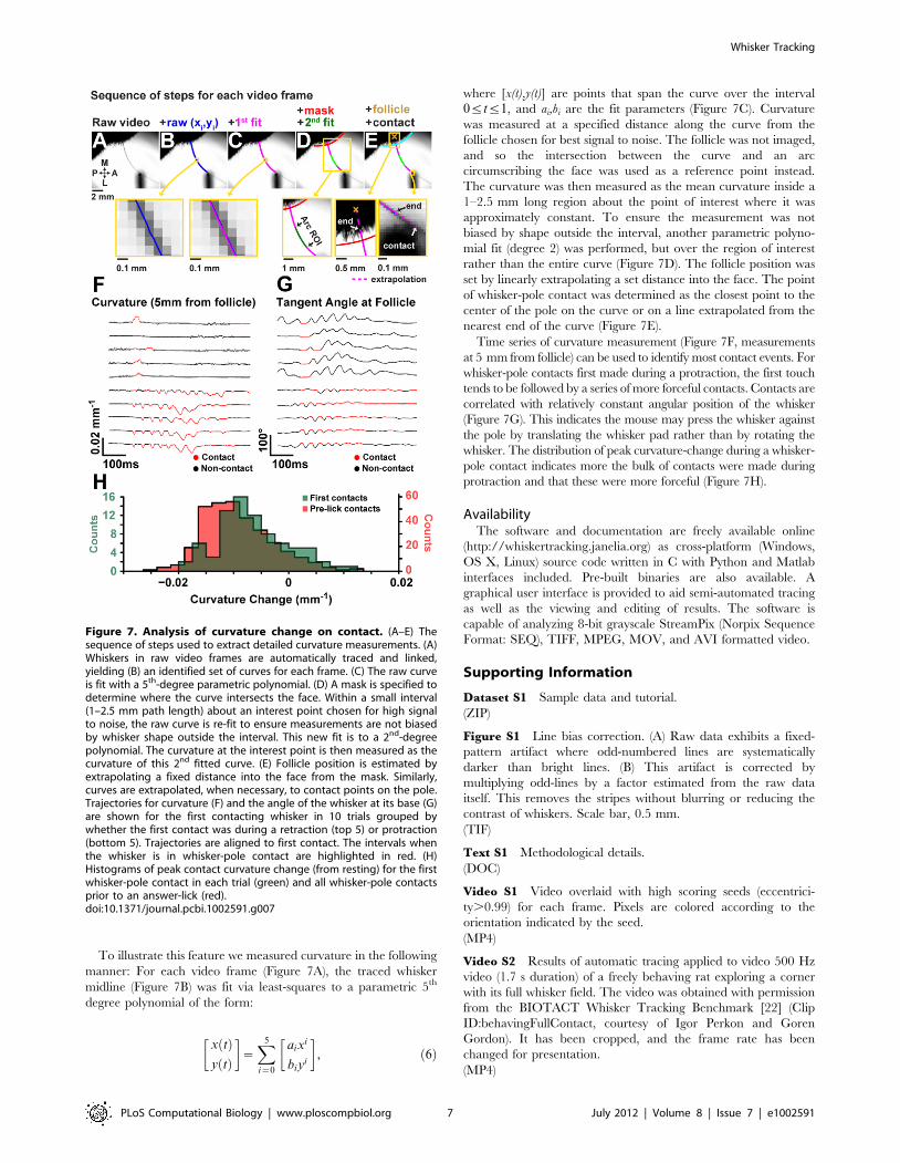
To illustrate this feature we measured curvature in the following
manner: For each video frame (Figure 7A), the traced whisker
midline (Figure 7B) was fit via least-squares to a parametric 5th
degree polynomial of the form:
x tð Þy tð Þ
� �~X5
i~0
aixi
biyi
� �, ð6Þ
where [x(t),y(t)] are points that span the curve over the interval
0ƒtƒ1, and ai,bi are the fit parameters (Figure 7C). Curvature
was measured at a specified distance along the curve from the
follicle chosen for best signal to noise. The follicle was not imaged,
and so the intersection between the curve and an arc
circumscribing the face was used as a reference point instead.
The curvature was then measured as the mean curvature inside a
1–2.5 mm long region about the point of interest where it was
approximately constant. To ensure the measurement was not
biased by shape outside the interval, another parametric polyno-
mial fit (degree 2) was performed, but over the region of interest
rather than the entire curve (Figure 7D). The follicle position was
set by linearly extrapolating a set distance into the face. The point
of whisker-pole contact was determined as the closest point to the
center of the pole on the curve or on a line extrapolated from the
nearest end of the curve (Figure 7E).
Time series of curvature measurement (Figure 7F, measurements
at 5 mm from follicle) can be used to identify most contact events. For
whisker-pole contacts first made during a protraction, the first touch
tends to be followed by a series of more forceful contacts. Contacts are
correlated with relatively constant angular position of the whisker
(Figure 7G). This indicates the mouse may press the whisker against
the pole by translating the whisker pad rather than by rotating the
whisker. The distribution of peak curvature-change during a whisker-
pole contact indicates more the bulk of contacts were made during
protraction and that these were more forceful (Figure 7H).
AvailabilityThe software and documentation are freely available online
(http://whiskertracking.janelia.org) as cross-platform (Windows,
OS X, Linux) source code written in C with Python and Matlab
interfaces included. Pre-built binaries are also available. A
graphical user interface is provided to aid semi-automated tracing
as well as the viewing and editing of results. The software is
capable of analyzing 8-bit grayscale StreamPix (Norpix Sequence
Format: SEQ), TIFF, MPEG, MOV, and AVI formatted video.
Supporting Information
Dataset S1 Sample data and tutorial.
(ZIP)
Figure S1 Line bias correction. (A) Raw data exhibits a fixed-
pattern artifact where odd-numbered lines are systematically
darker than bright lines. (B) This artifact is corrected by
multiplying odd-lines by a factor estimated from the raw data
itself. This removes the stripes without blurring or reducing the
contrast of whiskers. Scale bar, 0.5 mm.
(TIF)
Text S1 Methodological details.
(DOC)
Video S1 Video overlaid with high scoring seeds (eccentrici-
ty.0.99) for each frame. Pixels are colored according to the
orientation indicated by the seed.
(MP4)
Video S2 Results of automatic tracing applied to video 500 Hz
video (1.7 s duration) of a freely behaving rat exploring a corner
with its full whisker field. The video was obtained with permission
from the BIOTACT Whisker Tracking Benchmark [22] (Clip
ID:behavingFullContact, courtesy of Igor Perkon and Goren
Gordon). It has been cropped, and the frame rate has been
changed for presentation.
(MP4)
Figure 7. Analysis of curvature change on contact. (A–E) Thesequence of steps used to extract detailed curvature measurements. (A)Whiskers in raw video frames are automatically traced and linked,yielding (B) an identified set of curves for each frame. (C) The raw curveis fit with a 5th-degree parametric polynomial. (D) A mask is specified todetermine where the curve intersects the face. Within a small interval(1–2.5 mm path length) about an interest point chosen for high signalto noise, the raw curve is re-fit to ensure measurements are not biasedby whisker shape outside the interval. This new fit is to a 2nd-degreepolynomial. The curvature at the interest point is then measured as thecurvature of this 2nd fitted curve. (E) Follicle position is estimated byextrapolating a fixed distance into the face from the mask. Similarly,curves are extrapolated, when necessary, to contact points on the pole.Trajectories for curvature (F) and the angle of the whisker at its base (G)are shown for the first contacting whisker in 10 trials grouped bywhether the first contact was during a retraction (top 5) or protraction(bottom 5). Trajectories are aligned to first contact. The intervals whenthe whisker is in whisker-pole contact are highlighted in red. (H)Histograms of peak contact curvature change (from resting) for the firstwhisker-pole contact in each trial (green) and all whisker-pole contactsprior to an answer-lick (red).doi:10.1371/journal.pcbi.1002591.g007
Whisker Tracking
PLoS Computational Biology | www.ploscompbiol.org 7 July 2012 | Volume 8 | Issue 7 | e1002591

Video S3 Results of automatic tracing applied to a video
acquired at 100 Hz video (8 s duration) of a freely behaving mouse
with its full whisker field. Background subtraction was performed
before tracing to reduce the effects of non-uniform illumination.
Because no image of the scene without the animal present was
available, the background was estimated for each pixel as the
maximum intensity observed at that point throughout the video.
The video was obtained with permission from the BIOTACT
Whisker Tracking Benchmark [22] (Clip ID: behavingMouse100,
courtesy of Ehud Fonio and Ehud Ahissar). It has been cropped,
and the frame rate has been changed for presentation.
(MP4)
Video S4 Results from a full trial. The results of automated
tracing and linking applied to a video (500 Hz, 9.2 s duration) of a
head fixed mouse trimmed to a single row of 4 whiskers interacting
with a pole. Curves that were classified as whiskers are colored
according to their identity, and otherwise they are not shown.
Multiple whiskers simultaneously interact with the pole at 1.2–
1.4 sec into the trial. Protracted bouts of whisking can be observed
throughout the video.
(MP4)
Video S5 Tracing and linking is robust to rapid changes in
whisker angle. The results of automated tracing and linking
applied to a video (500 Hz, 150 ms) of a head fixed mouse
trimmed to a single row of 3 whiskers interacting with a pole.
Curves that were classified as whiskers are colored according to
their identity, and otherwise they are not shown. One whisker (red)
has been trimmed so it cannot contact the pole. The green whisker
presses against the pole, and quickly flicks past it as it is removed
from the field. This is the fastest angular motion (16u/ms) observed
in the data set used to measure tracking accuracy.
(MP4)
Video S6 Linking is robust to whiskers that leave the field of
view. The results of automated tracing and linking applied to a
video (500 Hz, 190 ms) of a head fixed mouse trimmed to a single
row of 3 whiskers interacting with a pole. Curves that were
classified as whiskers are colored according to their identity, and
otherwise they are not shown. Two whiskers (green and blue) are
frequently occluded by the lick-port (black bar, lower right), but
they are properly identified before and after such events.
(MP4)
Video S7 Tracing and linking of whiskers bilaterally. The results
of automated tracing and linking applied to a video (500 Hz, 1 s
duration) of a bilateral view to a head fixed mouse trimmed to a
single row of whiskers (2 on each side).
(MP4)
Author Contributions
Conceived and designed the experiments: NGC DHO KS EWM.
Performed the experiments: NGC DHO DH LP. Analyzed the data:
NGC DHO DH LP AH SP KS. Contributed reagents/materials/analysis
tools: NGC DHO DH LP. Wrote the paper: NGC KS EWM.
References
1. O’Connor DH, Clack NG, Huber D, Komiyama T, Myers EW, et al. (2010)Vibrissa-based object localization in head-fixed mice. J Neurosci 30: 1947–1967.
2. Knutsen PM (2006) Haptic Object Localization in the Vibrissal System:
Behavior and Performance. J Neurosci 26: 8451–8464.3. Carvell GE, Simons DJ (1990) Biometric analyses of vibrissal tactile
discrimination in the rat. J Neurosci 10: 2638–2648.4. Heimendahl von M, Itskov PM, Arabzadeh E, Diamond ME (2007) Neuronal
activity in rat barrel cortex underlying texture discrimination. Plos Biol 5: e305.
5. Mitchinson B, Martin CJ, Grant RA, Prescott TJ (2007) Feedback control inactive sensing: rat exploratory whisking is modulated by environmental contact.
Proc Biol Sci 274: 1035–1041.6. Diamond ME, Heimendahl von M, Knutsen PM, Kleinfeld D, Ahissar E (2008)
‘Where’ and ‘‘what’’ in the whisker sensorimotor system. Nat Rev Neurosci 9:
601–612.7. Hill DN, Bermejo R, Zeigler HP, Kleinfeld D (2008) Biomechanics of the
vibrissa motor plant in rat: rhythmic whisking consists of triphasic neuromus-cular activity. J Neurosci 28: 3438–3455.
8. Venkatraman S, Elkabany K, Long JD, Yao Y, Carmena JM (2009) A system forneural recording and closed-loop intracortical microstimulation in awake
rodents. IEEE Trans Biomed Eng 56: 15–22.
9. Jadhav SP, Wolfe J, Feldman DE (2009) Sparse temporal coding of elementarytactile features during active whisker sensation. Nat Neurosci 12: 792–2328.
10. Harvey MA, Bermejo R, Zeigler HP (2001) Discriminative whisking in the head-fixed rat: optoelectronic monitoring during tactile detection and discrimination
tasks. Somatosens Mot Res 18: 211–222.
11. Voigts J, Sakmann B, Celikel T (2008) Unsupervised whisker tracking inunrestrained behaving animals. J Neurophys 100: 504–515.
12. Ritt JT, Andermann ML, Moore CI (2008) Embodied information processing:Vibrissa mechanics and texture features shape micromotions in actively sensing
rats. Neuron 57: 599–613.
13. Knutsen PM, Derdikman D, Ahissar E (2005) Tracking whisker and head
movements in unrestrained behaving rodents. J Neurophys 93: 2294–2301.
14. Gyory G, Rankov V, Gordon G, Perkon I, Mitchinson B, et al. (2010) An
Algorithm for Automatic Tracking of Rat Whiskers. Proc Int Workshop on
Visual observation and Analysis of Animal and Insect Behavior (VAIB), Istanbul,
in conjunction with ICPR 2010: 1–4.
15. Perkon I, Kosir A, Itskov PM, Tasic J, Diamond ME (2011) Unsupervised
quantification of whisking and head movement in freely moving rodents.
J Neurophys 105: 1950–1962.
16. Birdwell JA, Solomon JH, Thajchayapong M, Taylor MA, Cheely M, et al.
(2007) Biomechanical models for radial distance determination by the rat
vibrissal system. J Neurophys 98: 2439–2455.
17. Huber D, Gutnisky DA, Peron S, O’Connor DH, Wiegert JS, et al. (2012)
Multiple dynamic representations in the motor cortex during sensorimotor
learning. Nature 484: 473–8.
18. Mehta SB, Whitmer D, Figueroa R, Williams BA, Kleinfeld D (2007) Active
spatial perception in the vibrissa scanning sensorimotor system. Plos Biol 5: e15.
19. Mikolajczyk K, Schmid C (2005) Performance evaluation of local descriptors.
IEEE Trans Pattern Anal Mach Intell 27: 1615–1630.
20. Torre V, Poggio TA (1986) On Edge Detection. IEEE Trans Pattern Anal Mach
Intell PAMI-8: 147–163.
21. Rabiner LR (1989) A tutorial on hidden Markov models and selected
applications in speech recognition. Proceedings of the IEEE. Vol. 77. pp.
257–286.
22. Gordon G, Mitcheson B, Grant RA, Diamond M, Prescot T, et al. (2012) The
BIOTACT Whisker Tracking Benchmark. Available:https://mushika.shef.ac.
uk/benchmark.
Whisker Tracking
PLoS Computational Biology | www.ploscompbiol.org 8 July 2012 | Volume 8 | Issue 7 | e1002591
Top Related