Asset Volatility

Maria Correia

London Business School

mcorreia@london.edu

Johnny Kang

AQR Capital Management LLC

johnny.kang@aqr.com

Scott Richardson

London Business School

srichardson@london.edu

February 13, 2014

Abstract

Asset volatility is a primitive variable in structural models of credit spreads. We

evaluate alternative measures of asset volatility using information from (i) historical

security returns (both equity and credit), (ii) implied volatilities extracted from equity

options, and (iii) financial statements. For a large sample of US firms, we find that

combining information from all three sources improves the explanatory power of

corporate bankruptcy models and cross-sectional variation in credit spreads. Market

based (accounting) measures of asset volatility appear to reflect systematic

(idiosyncratic) sources of volatility and combining both sources of information

generates a superior measure of total asset volatility that is relevant for understanding

credit spreads.

JEL classification: G12; G14; M41

Key words: credit spreads, volatility, bankruptcy, default.

We are grateful to Arne Staal and Philippe Vannerem at Barclays Capital for providing us access to the

Barclays Capital bond dataset. We also thank Cliff Asness, Max Bruche, John Campbell, John Hand,

Jens Hilscher, Ronen Israel, Anya Kleymenova, Sonia Konstantinidi, Caroline Pflueger, Tjomme

Rusticus and seminar participants at Cass Business School, London Business School, and University of

Porto for helpful discussion and comments. Richardson has an ongoing consulting relationship with

AQR Capital, which invests in, among other strategies, securities studied in this paper. The views and

opinions expressed herein are those of the authors and do not necessarily reflect the views of AQR

Capital Management, LLC (“AQR”) its affiliates, or its employees. This information does not

constitute an offer or solicitation of an offer, or any advice or recommendation, by AQR, to purchase

any securities or other financial instruments, and may not be construed as such.

1

1. Introduction

Our objective is to compare and contrast alternative measures of asset

volatility in their ability to explain security prices. A seminal paper by Merton (1974)

developed structural models as a benchmark to describe credit spreads. In these

models asset volatility is arguably the most important primitive variable for

determining distance to default and, consequently, spreads. In credit markets it is

total (i.e., both systematic and idiosyncratic) asset volatility that is relevant for

security prices (Campbell and Taksler, 2003). Thus, credit markets are a natural

setting to evaluate the relative importance of measures of asset volatility for security

pricing.

We examine three primary sources of information to measure asset volatility.

First, we extract information from secondary equity and credit markets to measure

equity volatility, debt volatility and their correlations. We derive several measures of

historical asset volatility ranging from simplistic deleveraging of historical equity

volatility to a complete measure that uses historical return volatilities and historical

return correlations (see e.g., Schaefer and Strebulaev, 2008). Second, we extract

information from equity option markets. Specifically, we use the implied volatility

for at the money put and call options. Third, we extract information from firm

financial statements about the volatility of firm’s unlevered profitability.

We find that combining information about asset volatility from market based

(historical and forward looking) and accounting based (historical) information

improves estimates of corporate bankruptcy.

Using a large sample of firms with liquid corporate bond data, we find that a

one standard deviation change in our market (accounting) based component measures

of asset volatility translates to an increase of 5.5 (2.5) percent in the conditional

2

probability of bankruptcy. We further find that market based and accounting based

estimates of asset volatility improve explanatory power of cross-sectional credit

spread regression models. Importantly, we show that regressing credit spreads onto a

constrained non-linear function of asset volatility and leverage – the credit spread

implied by the Merton model – performs significantly better than regressing onto

these variables linearly and independently. In constrained regression analysis where

we incorporate component measures of asset volatility into theoretically justified

implied spreads, we find that all component measures of asset volatility are relevant.

Specifically, historical market, forward looking market, and historical accounting

component measures of asset volatility account for 24.4%, 23.9%, and 19.0% of the

cross-sectional variation in credit spreads respectively. We also find some evidence

that the relative importance of accounting based measures of asset volatility is greatest

for high yield corporate bonds relative to investment grade bonds.

Measures of fundamental volatility have recently been examined in the context

of equity option markets (see e.g., Goodman, Neamtiu and Zhang, 2012 and Sridharan,

2012). A limitation of these analyses is that fundamental measures of volatility are

related to short dated (less than 90 day) straddle returns. Financial statements are

released at a quarterly frequency which makes them a slow moving source of

information about volatility. The credit instruments we examine (corporate bonds and

CDS) have considerably longer duration, thus making credit spreads a more natural

setting to examine the relative importance of market and accounting based component

measures of asset volatility.

Prior studies have documented an association between idiosyncratic equity

(Campbell and Taksler, 2003) and bond (Gemmil and Keswani, 2011) volatility and

credit spreads at an aggregate and issuer level. Taking these findings into account and

3

to help better understand the relative importance of market based and accounting

based component measures of asset volatility we explore the mapping of these

respective measures to systematic and idiosyncratic volatility. We find that average

within industry pairwise correlations of market measures of returns (both equity and

credit market returns) are significantly larger than within industry pairwise

correlations of changes in seasonally adjusted accounting rates of return. This

suggests that market based measures of asset volatility are more likely to reflect

systematic sources of volatility. To further explore this possibility, we form factor

mimicking portfolios based on market and accounting based measures of asset

volatility. We find that the market based asset volatility factor mimicking portfolio

has a significantly higher beta with respect to aggregate asset returns. Together this

evidence suggests that combining measures of asset volatility from market based and

accounting based measures yields a superior measure of asset volatility due to a

combination of systematic and idiosyncratic measures of asset volatility. This finding

is consistent with the two different sources of firm-level return volatility identified by

(Vuolteenaho 2002), cash flow news, which are largely firm-specific, and expected

return news, with a stronger systematic component. As discussed earlier, in the

context of credit derivatives total asset volatility is the relevant measure, and not just

systematic volatility.

The rest of the paper is structured as follows. Section 2 describes our sample

selection and research design. Section 3 presents our empirical analysis and

robustness tests, and section 4 concludes.

4

2. Sample and research design

2.1 Secondary credit market data

Our analysis is based on a comprehensive panel of US corporate bond data,

which includes all the constituents of (i) Barclays U.S. Corporate Investment Grade

Index, and (ii) Barclays U.S. High Yield Index. The data includes monthly returns and

bond characteristics from September 1988 to February 2013. We exclude financial

firms, with SIC codes between 6000 and 6999. Table 1, Panel A shows the industry

composition of the resulting sample, using Barclays Capital’s industry definitions.

Approximately 35% of the sample firms are consumer products firms. Capital Goods

firms and Basic Industry make up for another 20% of the sample.

2.2 Representative bond

Given that corporate issuers often issue multiple bonds and that our analysis is

directed at measuring asset volatility of the issuer, we need to select a representative

bond for each issuer. To do this, we follow the criteria in Haesen, Houweling and

VanZundert (2012). We repeat this exercise every month for our sample period. The

criteria used for identifying the representative bond are selected so as to create a

sample of liquid and cross-sectionally comparable bonds. Specifically, we select

representative bonds on the basis of (i) seniority, (ii) maturity, (iii) age, and (iv) size.

First, we filter bonds on the basis of seniority. Because most companies issue

the majority of their bonds as senior debt, we select only bonds corresponding to the

largest rating of the issuer. To do this we first compute the amount of bonds

outstanding for each rating category for a given issuer. We then keep only those

bonds that belong to the rating category which contains the largest fraction of debt

outstanding. This category of bonds tends to have the same rating as the issuer.

5

Second, we then filter bonds on the basis of maturity. If the issuer has bonds with time

to maturity between 5 and 15 years, we remove all other bonds for that issuer from the

sample. If not, we keep retain all bonds in the sample. Third, we then filter bonds on

the basis of time since issuance. If the issuer has any bonds that are at most two years

old, we remove all other bonds for that issuer. If not, we keep all bonds from that

issuer in the sample. Finally, we filter on the basis of size. Of the remaining bonds,

we pick the one with the largest amount outstanding.

Our resulting sample includes 121,612 unique bond-month observations,

corresponding to 6,084 bonds issued by 1,547 unique firms. Sample bonds have an

average option adjusted spread (OAS) of 3.33% over the sample period, and an

average option adjusted duration (OAD) of 5.16 years (Table 1, Panel B).

2.3 Measures of asset volatility

2.3.1 Historical market data

We calculate historical equity volatility using the annualized standard

deviation of CRSP realized daily stock returns over the past 252 days, ��.

We use market leverage to de-lever historical equity volatility and obtain our

first measure of asset volatility:

������� = �� ��� (1)

where E is the market value of the firm’s equity and X is the book value of short term

debt plus half of the book value of long term debt (e.g., Bharath and Shumway, 2008).

Our second estimate of historical asset volatility, �� , combines historical

credit and equity market data:

��=�� �� + (1 − �) �� + 2��,����� (2)

6

where � = ��� is the fraction of asset value attributable to equity, �� is the standard

deviation of total monthly bond returns from Barcap and ��,� is an estimate of the

historical correlation between equity and bond returns. We compute the correlation

between equity and bond returns for each bond in the representative sample over a 12

month period. Note that while our selection of a representative bond can change each

month for a given issuer, our correlation and volatility measures hold a given bond

fixed when looking back in time.

To mitigate noise in our estimate of historical correlations, we shrink our

estimate of correlation to the average correlation for a given level of credit risk (see

e.g., Lok and Richardson, 2011). Specifically, we compute ��,� for each issuer as the

average correlation for all firms in the same decile of option adjusted credit spread.

In untabulated robustness tests, we also examine a Merton distance to default

model estimate of asset volatility, following Bharath and Shumway (2008). This

volatility is computed by simultaneously solving the Black-Scholes-Merton system of

equations, using a numerical algorithm with historical volatility as a starting point.

Table 1, Panel B presents descriptive statistics for the variables used to

deleverage volatility. Sample firms have an average market leverage of approximately

27% (1-0.7324) and exhibit an average correlation between equity and debt returns

��,� of 0.2284. We winsorize �� , �������, and �� at the 1st and 99

th percentile values

of their respective distribution.

The Appendix defines these variables, as well as other variables used in the

paper, in more detail.

2.3.2 Forward looking market data

7

We obtain implied Black-Scholes volatility estimates for at-the-money 91-day

call options from the OptionMetrics Ivy DB standardized database.1 We average the

implied volatility for a 91-day put and call option. Based on this implied equity

volatility, �� , we compute two asset volatility estimates, �������� and ���� , using the

approaches in (1) and (2), respectively. We winsorize �������� and ���� at their

respective 1st and 99

th percentile values. Option implied volatility has been shown to

have incremental power with respect to historical volatility in explaining time-series

and cross-sectional variation in credit spreads (Cremers et al., 2008; Cao et al., 2010).

2.3.3 Fundamental data

We use two approaches to compute measures of fundamental volatility. Both

approaches are designed to measure volatility of unlevered profitability, RNOA. First,

we use the quantile regression approach described in Konstantinidi and Pope (2012)

and Chang, Monahan and Ouazad (2013). Second, we use a simple approach based

on historical volatility of seasonally adjusted RNOA.

2.3.3.1 Quantile regression approach

This approach consists of using quantile regressions to estimate the quantiles

and conditional moments of the RNOA distribution. Following Konstantinidi and

Pope (2012) and Chang, Monahan and Ouazad (2013), we exclude financial firms

with SIC codes 6000 to 6999. We estimate coefficients for each percentile using an

expanding window approach starting in 1963. In particular, for each year t, we

estimate the following regression, using quarterly data from 1963 to t:

1 The standardized implied volatilities are calculated by OptionMetrics using linear interpolation from

their Volatility Surface file.

8

������� �!�",#$ ∙& = '(,#� + '),#� �!�",#*) + ' ,#� +!,,",#*) + '-,#� �+!,,",#*) × �!�",#*)& + '/,#� �00",#*) + '1,#� 2�34 ",#*) + '5,#� 2�3!��",#*) (3)

This model is similar to the model in Chang et al. (2013) and Hou, Van Dijk, and

Zhang (2012), with the exception that we forecast return on net operating assets

(RNOA) instead of return on equity (ROE) and therefore do not include Leverage as

an explanatory variable and scale all variables by the average balance of net operating

assets (NOA) rather than by the average balance of equity. RNOA is operating income

(‘OIADPQ’) scaled by the average balance of NOA. NOA is defined as the sum of

common equity, preferred stock, long term debt, debt in current liabilities and

minority interests minus cash and short term investments

(‘CEQQ’+’PSTKQ’+’DLTTQ’+DLCQ’+’MIBQ’-‘CHEQ’). LOSS is an indicator

variable equal to 1 if RNOA is negative and 0 otherwise. ACC are the accruals

reported by the firm (∆’ACTQ’-∆‘CHEQ’-(∆’LCTQ’-∆’DLCQ’-∆‘TXPQ’)-‘DPQ’).

PAYOUT is the dividends paid by the firm (‘DVPSX_F’). PAYER is an indicator

variable equal to 1 if the firm distributed dividends, i.e. PAYOUT>0, 0 otherwise. We

compute these variables at the end of each quarter, using the most recent four quarters

of data.

In unreported analyses, we find the expected relations between our included

explanatory variables and future profitability. Specifically, the median quantile

regression generates the following results: (i) ')1( is 0.94 consistent with mean

reversion in accounting rates of return (e.g., Penman, 1991, and Fama and French,

2000), (ii) ' 1( is -0.01 consistent with loss makers having lower levels of future

profitability (e.g., Hou, Van Dijk, and Zhang, 2012), (iii) '-1( is -0.14 consistent with

faster mean reversion in profitability for loss making firms (e.g., Beaver, Correia and

McNichols, 2012), (iv) '/1( is -0.02 consistent with the well documented negative

9

relation between accruals and future firm performance (e.g., Sloan, 1996, and

Richardson, Sloan, Soliman and Tuna, 2006), (v) '11( is 0.02 consistent with dividend

paying firms having higher levels of future profitability (e.g., Hou, Van Dijk, and

Zhang, 2012), and (vi) '51( is 0.26 also consistent with firms with higher dividend

payout having higher levels of profitability (e.g., Hou, Van Dijk, and Zhang, 2012).

We combine the values of the independent variables in year t with the vector

of coefficients, Ɓ#�='(,#� , … , '5,#� to obtain out-of-sample estimates of the percentiles

for the year t+1. In particular, we obtain a vector of coefficient estimates,Ɓ#�8 , for each

percentile and sample quarter. Based on this vector, we estimate the expected value of

each of the 100 percentiles as 4(9#�)|;#)< = Ɓ#�8;# . For purposes of estimation of the vector of coefficient estimates, we delete

extreme observations of dependent and independent variables. In particular, we delete

all observations with $ �!�",#$>2, $ �!�",#*)$>2, $�00",#*)$>2, $2�3!��",#*)$>1,

$2�3!��",#*)$<0.

We focus on two measures of conditional volatility for each firm, and year t.

The standard deviation of the distribution of quantile estimates,

�= = ,>?�4(9#�)|;#)< &, q=1,…, 100, and the difference between the predicted value

of the 95th

percentile and the predicted value of the 5th

percentile, 29525 =4(95#�)|;#)< −4(5#�)|;#)< .

2.3.3.2 Naïve approach

For each quarter we compute RNOA as operating income (‘OIADPQ’) to

average NOA during the quarter. We estimate the volatility of RNOA, �=�����, as the

standard deviation of seasonally adjusted RNOA over the previous 5 years (20

10

quarters), requiring at least 10 available quarterly observations. Seasonally adjusted

RNOA for quarter k in year t is computed as2:

�!�#,BC� = �!�#,B − �!�#*),B (4)

We then compute the standard deviation of seasonally adjusted RNOA over

the previous 5 years, requiring a minimum of 10 quarters of data.

�=����� = ,>?( �!�#,BC�) (5)

Table 1, Panel C reports descriptive statistics for the different volatility

measures. These measures exhibit differences in scale. In particular, volatility

measures based on financial statement information, �=����� and �= , are lower, on

average, than asset volatility measures based on naïve or weighted deleveraging of

historical equity returns or implied equity volatility. We discuss how we deal with

differences in scale below when combining our component measures of asset

volatility in section 3.2.2.

Panel D of Table 1 reports the average monthly pairwise correlations across

volatility measures. Historical equity volatility, ��, is highly correlated with implied

volatility, �� , [0.8822 (0.9013) Pearson (Spearman) correlation]. The Pearson

(Spearman) correlation between these equity volatility measures and debt volatility,

�� , ranges between 0.3769 and 0.4732 (0.2662 and 0.3381). As a result, the

correlations between weighted asset volatilities and the corresponding equity

volatility measures are, on average lower than 0.80.

Correlations between accounting based (�=, �=�����, and 29525) and market

based asset volatility measures (���, ������� , ����and ��������) are much lower. The

2 As an alternative naïve approach, we estimate a time-series model for RNOA and calculate the time-

series volatility only for the residual (the stationary component). In particular, we estimate the

following regression for each firm: �!�# = '( + ') �!�#*) +∑ '�E�# + F#/�G .

11

maximum pairwise Pearson (Spearman) correlation between these two types of

measures is 0.2491 (0.4223) and the minimum 0.1538 (0.2201).

2.4 Bankruptcy data and distance to default

We estimate the probability of bankruptcy based on a sample of Chapter 7 and

Chapter 11 bankruptcies filed between 1980 and the end of 2012. We combine

bankruptcy data from four main sources: Beaver, Correia, and McNichols (2012)

(BCM)3; the New Generation Research bankruptcy database (bankruptcydata.com);

Mergent FISD; and the UCLA-Lo Pucki bankruptcy database.

Following Shumway (2001), we winsorize all independent variables at 1% and

99%. To ensure that prediction is made out of sample and to avoid a potential bias of

ex post over-fitting the data, we estimate coefficients using an expanding window

approach.4

We convert the different scores into probabilities as follows:

Prob=escore

/1+escore

.

Following Correia, Richardson and Tuna (2012) we use quarterly financial

data to compute the default barrier and update market data on a monthly basis to

obtain monthly estimates of the probabilities of bankruptcy. Market variables are

measured at the end of each month and accounting variables are based on the most

recent quarterly information reported before the end of the month. We ensure that all

3 Beaver, Correia, and McNichols (2012) combine the bankruptcy database from Beaver, McNichols,

and Rhie (2005), which was derived from multiple sources including CRSP, Compustat,

Bankruptcy.com, Capital Changes Reporter, and a list provided by Shumway with a list of bankruptcy

firms provided by Chava and Jarrow and used in Chava and Jarrow (2004).

4 In particular, to estimate the probability of bankruptcy for calendar year 2011 (January 2011 to

December 2011), we combine all the available accounting and market data from January 1980 to

December 2009, use it to predict bankruptcy outcomes for January 1981 to December 2010, retain the

coefficients, and use them to estimate the probability of bankruptcy for 2011. To obtain an estimate of

the probability of bankruptcy for the period from February 2011 to January 2012, we include one more

month in the estimation. In particular, we combine all the available accounting and market data from

January 1980 to January 2010, use it to predict bankruptcy outcomes for January 1981 to January 2011,

and apply the estimated coefficients to accounting and market data available at January 2011.

12

independent variables are observable before the declaration of bankruptcy. Our

dependent variable is equal to 1 if a firm files for bankruptcy within 1 year of the end

of the month. Following prior literature, we keep the first bankruptcy filing and

remove from the sample all months after this filing.

Following Shumway (2001), we estimate probabilities of bankruptcy by using

a discrete time hazard model and including three types of observations in the

estimation: nonbankrupt firms, years before bankruptcy for bankrupt firms, and

bankruptcy years. All of the models are nonlinear transformations of various

accounting and market data.

The primary regression model for estimating bankruptcy over the next twelve

months is as follows:

Pr(3#�) = 1) = J KLM N�OOP , 4QRS>#, LM(4#), �B,#T (6)

The dependent variable is equal to 1 if the firm filed for bankruptcy within the

following year. LM N�OOP is a measure of dollar distance to default barrier (akin to an

inverse measure of leverage). We compute U# as the sum of the market value of the

firm’s equity and the book value of debt. We compute our default barrier,;#, as the

sum of short-term debt (‘DLCQ’) and half of long-term debt (‘DLTTQ’) as reported

at the most recent fiscal quarter (see e.g., Bharath and Shumway, 2008).4QRS># is the

excess equity return over the risk free rate for the most recent 12 months. LM(4#) is

the log of the market value of equity measured at the start of the forecasting month.

�B,# is the respective measure of asset volatility as defined in section 2.3. We estimate

equation (6) using various combinations of our measures of asset volatility over

different samples to assess the relative importance of market based and accounting

based measures of asset volatility in the context of forecasting bankruptcy.

13

Our priors for equation (6) are as follows: (i) LM N�OOP is expected to be

negatively associated with bankruptcy likelihood (the further the market value of

assets is from the default barrier the lower the likelihood of hitting that barrier in the

next twelve months), (ii) 4QRS># is expected to be negatively associated with

bankruptcy likelihood (assuming there is information content in security prices,

decreases in security prices should be associated with increased bankruptcy

likelihood), (iii) LM(4#) is expected to be negatively associated with bankruptcy

likelihood (this is a well-known empirical relation but the ex-ante justification is less

clear, some argue that large firms offer better diversification and better realizations of

asset values in the event of default), and (iv) �B,# is expected to be positively

associated with bankruptcy likelihood (the greater the volatility of the asset value the

greater the chance of passing through the default barrier).

2.5 Theoretical Credit Spreads

Our next empirical prediction is dependent on the success of the respective

measures of asset volatility in forecasting bankruptcy in the context of equation (6).

Given that a measure of asset volatility is useful in forecasting bankruptcy, and under

the assumption that security prices in the secondary market are reasonably efficient,

we test whether different combinations of measures of asset volatility are able to

better explain cross-sectional variation in credit spreads.

We do this analysis with two approaches. First, we estimate an unconstrained

cross-sectional regression where we include multiple measures of determinants of

credit spreads in a linear model. Second, we estimate a constrained cross-sectional

regression where we combine our various measures of asset volatility into measures

of distance to default which are in turn mapped to an implied credit spread. A benefit

14

of the constrained approach is that it combines the dollar distance to default, LM N�OOP,

with measures of asset volatility, �B,#, to better identify closeness to the default barrier.

An unconstrained regression is unable to capture the inherent non-linearity in distance

to default.

For the unconstrained approach we estimate the following regression model:

!�,# = V)LM N�OOP + V 4QRS># + V-LM(4#) + ∑ VB�-�B,#WBG) + X0YM>RYL# + F# (7)

!�,# is the option adjusted spread for the respective bond as reported in the

Barclays Index. An intercept is not reported as we include time fixed effects. In

addition to the determinants of bankruptcy, i.e., LM N�OOP, 4QRS># , LM(4#), and �B,# ,

which are all issuer level determinants of credit risk, we also include issue specific

determinants of credit risk that will influence the level of credit spreads. Specifically,

our additional controls include: (i) Z>[M\# which is the issue specific rating (higher

rated issues are expected to have higher credit spreads, given that we code ratings to

be increasing in risk), (ii) �\S# is the time since issuance (liquidity is decreasing for

progressively ‘off the run’ securities, so we expect credit spreads to be increasing in

time since issuance), and (iii) ]^RZ>[YM# is option adjusted duration of the issue (for

the vast majority of corporate issuers the credit term structure is upward sloping so we

expect credit spreads to increase with duration, see e.g., Helwege and Turner, 1999).

For our constrained approach, we first combine our measures of the dollar

distance to default, LM N�OOP, and the respective measures of asset volatility, �B,# , to

construct a measure of expected distance to default. This distance to default is then

empirically mapped to our bankruptcy data to generate a forecast of physical

bankruptcy probability, labelled as 4�2]"#B&. We estimate this physical bankruptcy

probability for each of our asset volatility measures according to equation (8) below:

15

4�2]"#B& = J _`abcd,efd.Ohc,O√# j (8)

We next convert each physical bankruptcy probability into a risk-neutral

measure, following the approach described in Kealhofer (2003) and Arora, Bohn, and

Zhu (2005). We first cumulate our physical bankruptcy probability, 02]",#B . It is

computed directly from 4�2]"#B& by cumulating survival probabilities over the

relevant number of periods. In particular, 02]",#B = 1 − N1 − 4�2]"#B&Pk . We then

convert this cumulative physical bankruptcy probability, 02]",#B , to a cumulative risk

neutral bankruptcy probability, 0�]l",#B . We use a normal distribution to convert

physical probabilities of bankruptcy to risk neutral probabilities, following the

approach in Crouhy, Galai, and Mark (2000), Kealhofer (2003); and Arora, Bohn and

Zhu (2005):

0�]l",#B = � m�*)n02]",#B o + p�R",# √�q (9)

The cumulative physical bankruptcy probability is first converted into a point

in the cumulative normal distribution. A risk premium is then added. The risk

premium is the product of (i) the issuers sensitivity to the market price of risk, as

measured by the correlation between the underlying issuer level asset returns and the

market index return, �R",# , (ii) the market price of risk (i.e. the market Sharpe ratio,

measured by λ), and (iii) the duration of the credit risk exposure, T. The risk modified

physical bankruptcy probability is then mapped back to risk neutral space. We set the

market Sharpe ratio, λ, equal to 0.5, consistent with the values observed by Kealhofer

(2003). We set �R",# equal to the correlation between monthly firm stock returns and

monthly market returns using a rolling 60 month window. We impose a floor (ceiling)

16

on the estimated correlation at 0.1 (0.7).Finally, we estimate implied (or theoretical)

credit spreads as follows:

0,",#B = − )k LMn1 − �1 − ",#&0�]l",#B o (10)

",# is expected recovery rate conditional on bankruptcy, which we set equal to

0.4 for all firms. While we assume ",# to be a constant, it is possible that recovery

rates exhibit systematic time-variation (Bruche and Gonzales-Aguado, 2009). While

this could affect the gap between theoretical and observed credit spreads, we have no

reason to believe it will present a concern to our analysis, given that we do not

examine this gap directly.

For the constrained approach, we then estimate the following regression

model:

!�,# = V)4QRS># + V LM(4#) + ∑ VB� WBG) 0,hr,O + X0YM>RYL# + F# (11)

Table 1, Panel E reports the average pairwise correlations between the

observed credit spread, !�,# , and the theoretical credit spreads based on each

volatility measure. Correlations between accounting based (0,hs , 0,tu1t1, 0,hsvcwbx) and

market based (0,hcvcwbx, 0,hcy , 0,hcwvcwbx, 0,hcwy ) credit spreads are substantially higher than

correlations between the corresponding volatility measures, reported in Panel D. In

particular, accounting based credit spreads exhibit an average Pearson (Spearman)

correlation of 0.8966 (0.7204), which contrasts with an average Pearson (Spearman)

correlation of 0.1921(0.2962) between the respective volatility measures. The

reported difference in the magnitude of correlations is as expected given that

theoretical credit spreads embed common additional information such as leverage.

Theoretical spreads based on historical security data or option implied

volatility exhibit higher correlation with observed spreads than theoretical spreads

based on accounting data. In particular, !�,# exhibits an average Pearson (Spearman)

17

correlation with accounting based spreads (0,hs , 0,tu1t1, 0,hsvcwbx) of 0.7002 (0.5333),

and an average Pearson (Spearman) correlation of 0.7704 (0.7230) with market based

spreads (0,hcvcwbx , 0,hcy , 0,hcwvcwbx , 0,hcwy ).

3. Results

3.1 Bankruptcy forecasting

Table 2 reports the estimation results of regression equation (6). Across all

specifications we find expected relations for our primary determinants: bankruptcy

likelihood is decreasing in (i) distance to default barrier, LM N�OOP, (ii) recent equity

returns, 4QRS>#, and (iii) firm size, LM(4#). To assess the relative importance of our different component measures of asset

volatility, we first examine each measure individually after controlling for the same

issuer level determinants of bankruptcy. Across models (1) to (5) in Table 2 we find

that all of the component measures of asset volatility are significantly positively

associated with the probability of bankruptcy. These regression specifications are

unconstrained so we include each of the respective component measures of asset

volatility separately and do not attempt to combine together different volatility

measures. In our constrained specifications later we combine the component measures

of asset volatility together.

To provide a sense of the relative economic significance across the component

measures of asset volatility, we report in panel B of Table 2 the marginal effects for

each explanatory variable. Specifically, we hold each explanatory variable at its

average value and report the change in probability of bankruptcy for a one standard

deviation change for the respective explanatory variable relative to the full sample

unconditional probability of bankruptcy. For example, column (1) in panel B of

Table 2 states that the marginal effect of �� is 0.0256. This means that a one standard

18

deviation change in �� is associated with a 2.56% increase in bankruptcy probability,

relative to the full sample unconditional probability of bankruptcy (0.61%).

Comparing marginal effects across explanatory variables reveals that distance to

default barrier and recent equity returns appear to be the most economically important

explanatory variables. Individually, the most important component measure of asset

volatility is �� (marginal effect of 0.0624 is the largest in the first 5 columns of panel

B of Table 2).

Models (6) to (9) in Table 2 combine different component measures of asset

volatility. We do not include �� and �� in the same specification due to multi-

collinearity (panel D of Table 1 shows that �� and �� have a parametric correlation of

0.8822). In model (6) we start with issuer level determinants (LM N�OOP, 4QRS>#, and

LM(4#)) and �� . We then add a measure of volatility from the credit markets, �� .

Combining market based measures of asset volatility from the equity and credit

markets is superior to examining equity market information alone (the pseudo-R2

increases from 29.35 percent in model (2) to 29.78 percent in model (6)). Panel B of

Table 2 shows that the scaled marginal effect for �� is 30 percent as large as that for

��. In model (7) when we add our first measure of fundamental volatility, �=, we find

that all three component measures of volatility are significantly associated with

bankruptcy. In terms of relative economic significance, �� is 30 percent as large as

that for ��, and �= is 46 percent as large as that for ��. Using alternative measures of

fundamental volatility in models (8) and (9) we find similar results: combining

measures of volatility from market and accounting sources improves explanatory

power of bankruptcy prediction models. In untabulated robustness analysis, we

document further that our fundamental volatility measures also improve the

19

explanatory power of a bankruptcy prediction model that includes Merton-based

volatility and leverage measures (see e.g., Bharath and Shumway, 2008).

3.2 Cross-sectional variation in credit spreads

3.2.1 Unconstrained analysis

Having established the information content of our candidate component

measures of asset volatility for bankruptcy prediction, we now turn to assess the

information content of the same measures for secondary credit market prices. As

discussed in section 2.5, under the assumption that security prices in the secondary

market are reasonably efficient, we expect to see that the determinants of bankruptcy

prediction models should also be able to explain cross-sectional variation in credit

spreads.

Table 3 reports estimates of equation (7). This is our unconstrained analysis

of how, and whether, different component measures of asset volatility have

information content for security prices. We include month fixed effects to control for

macroeconomic factors, and as such we do not report an intercept. As discussed in

section 2.5, we include additional issue specific measures ( Z>[M\# , �\S# , and

]^RZ>[YM#) to help control for other known determinants of credit spreads. Of course,

it is possible that we are ‘throwing the baby out with the bath water’ by including

these determinants, especially Z>[M\# . For example, the rating agencies may be

using algorithms to assess credit risk that spans accounting and market data sources,

and as such included rating categories might subsume the ability of this data to

explain cross-sectional variation in credit spreads. In unreported analysis, we find

that our inferences of the combined information content of market and accounting

20

based information to measure asset volatility is unaffected by the inclusion of

Z>[M\#. Across all models estimated in Table 3 we find expected relations for our

primary determinants. Credit spreads are consistently decreasing in (i) distance to

default barrier, LM N�OOP, and (ii) firm size, LM(4#). Credit spreads are consistently

increasing in (i) credit rating (scaled to take higher values for higher yielding issues),

Z>[M\#, and (ii) time since issuance, �\S#. Recent excess equity returns, 4QRS>#, is

usually negative across different models but is rarely significant at conventional levels.

Option adjusted duration, ]^RZ>[YM# , is either negatively or positively associated

with credit spreads: its effect is dependent upon the included explanatory variables

(once �� is included the relation turns negative).

Models (1) to (6) in Table 3 examine each of our component measures of asset

volatility separately. Individually, each of our component measures of asset volatility

is significantly positively associated with credit spreads. To provide a sense of the

relative economic significance across the component measures of asset volatility, we

also report in panel B of Table 3 the marginal effects for each explanatory variable.

Similar to the marginal effects reported in Table 2, we report the change in credit

spreads for a one standard deviation change for the respective explanatory variable

relative to the full sample unconditional mean credit spread. Individually, the most

important component measure of asset volatility is �� (marginal effect of 0.6262 is the

largest in the first 6 columns of panel B of Table 3).

Models (7) to (10) in Table 3 combine different component measures of asset

volatility. As in Table 2, we do not include �� and �� in the same specification due to

multi-collinearity concerns. In model (7) we add a measure of volatility from the

credit markets, ��. Consistent with the results in Table 2, combining market based

21

measures of asset volatility from the equity and credit markets is superior to

examining equity market information alone (the R2 increases from 67.0 percent in

model (2) and 67.1 percent in model (6) to 72.3 percent in model (7)). Panel B of

Table 3 shows that the scaled marginal effect for �� is 81 percent as large as that for

��. In model (8) when we add our first measure of fundamental volatility, �=, we find

that all three component measures of volatility are significantly associated with

bankruptcy, but that the relative importance of �= is quite low. In terms of relative

economic significance, �� is 81 percent as large as that for �� , and �= is only 4

percent as large as that for ��. Using alternative measures of fundamental volatility in

models (9) and (10) we find similar results: combining measures of volatility from

market and accounting sources improves explanatory power of credit spreads. In

untabulated sensitivity tests, we document further that this finding is robust to the use

of a Merton-based volatility measure estimated following Bharath and

Shumway(2008).

Table 4 reports the results of equation (7) where we allow the regression

coefficients to vary for Investment Grade (IG) and High Yield (HY) issuers. For the

sake of brevity we only report the differential coefficients for HY issuers. As

expected the HY indicator variable is strongly significantly positive reflecting the

higher risk of HY issuers relative to IG issuers. Across the various specifications

there is consistent evidence that the primary determinants of credit spreads are

stronger for HY issuers: credit spreads are more strongly decreasing in firm size,

distance to default and recent excess equity returns for HY issuers relative to IG

issuers. We find that market based component measures of asset volatility, �� and ��, are also more strongly associated with credit spreads for HY issuers. Finally, there is

only weak evidence that component measures of asset volatility based on

22

fundamentals are more important for HY issuers (only the naïve measure, �=�����, is

significant across models (8) to (10) in panel A of Table 4).

3.2.2 Constrained analysis

We now assess the relative information content of the different component

measures of volatility in a constrained specification. As described in section 2.5 and

equation (8), we combine component measures of asset volatility with dollar distance

to default to identify a distance to default barrier in standard deviation units. We then

calibrate the various distance to default measures to an expected physical default

probability which is converted to an implied spread as per equations (9) and (10). We

thus generate k different theoretical spreads where the difference is attributable to the

use of different component measures of volatility. This approach is arguably superior

to the unconstrained analysis discussed in section 3.2.1 because of the inherent non-

linearity between dollar distance to default barrier and asset volatility. Two firms

could have the same dollar distance to default but typically vary in terms of asset

volatility. It is the ratio of these two measures that matters for determining physical

bankruptcy probability, not the two measures separately.

An empirical challenge that we face is combining different component

measures of volatility that vary in scale. As can be seen from panel C of Table 1, the

market based component measures of asset volatility have higher average values and

higher standard deviations relative to the accounting based measures of asset volatility.

To handle these differences in scale when we combine component measures of asset

volatility we first standardize each accounting based component measure and rescale

them such that they have the same mean and standard deviation as the market based

component measures of asset volatility to which they will be combined with. As a

23

result of this process we end up with seven different measures of theoretical spreads.

We have four market based theoretical spreads: (i) 0,hx which is based on historical

equity volatility alone, (ii) 0,hd which is based on implied equity volatility alone, (iii)

0,hcz which is based on a weighted combination of historical equity volatility and

historical credit volatility, and (iv) 0,hcwz which is based on a weighted combination of

implied equity volatility and historical credit volatility. We have three accounting

based theoretical spreads: (i) 0,hs which is based on a parametric estimate of

fundamental volatility, (ii) 0,tu1t1 which is based on a non-parametric estimate of

fundamental volatility, and (iii) 0,hsvcwbx which is based on historical fundamental

volatility.

Table 5 reports regression results of equation (11). We retain the same set of

controls and explanatory variables to allow comparability of explanatory power

between equation (7) and equation (11). We include a set of month fixed effects and

as such do not report a regression intercept. Model (1) shows that theoretical spreads

based on a simple measure of historical equity volatility is able to explain 71.5

percent of the variation in credit spreads, and the regression coefficient on 0,hx{�C� is

0.567. A regression coefficient less than one may suggest that our measure of

theoretical credit spread is larger than the actual market spread. This is not the case as

our regression model includes an intercept (via time fixed effects). In unreported

analysis, if we exclude fixed effects, and other control variables, we find that the

regression coefficient on 0,hx{�C� is statistically greater than one, consistent with the

well-known result that structural models tend to under forecast credit spreads (e.g.,

Huang and Huang, 2008).

Before assessing the incremental improvement in explanatory power from

alternative component measures of asset volatility, we first use our secondary credit

24

market data to apply a ‘hair-cut’ to the book value of debt used as an approximation

for the market value of assets. While fixed and floating rate debt is usually issued at

par, over time changes in credit risk of the issuer tend to create situations where the

market value of debt is below the book value of debt, thus our estimate of market

value of assets is likely to be too high. A consequence of this is that any implied

spread will be too low. To correct for this error we take a fraction of the book value

of debt as our approximation for the market value of debt using the current credit

spread on the representative bond we have selected for each issuer. Specifically, we

multiple the book value of debt by )()�|�C)}, which assumes an average duration of

around five years which is consistent with the average option adjusted duration for

our sample as reported in panel B of Table 1. Model (2) of Table 5 shows that once

we incorporate this ‘hair-cut’ we observe a noticeable change in explanatory power.

The R2 in model (2) increases to 76.6 percent from 71.5 percent for model (1).

Models (3) to (12) in Table 5 consider various combinations of our theoretical

spreads. When we include both historical and forward looking equity volatility

information in model (4) we find that historical equity dominates. More importantly,

in model (6) when we include theoretical spreads based on combined component

measures of asset volatility we see that both historical equity volatility and forward

looking equity information are important. For the sake of brevity, we do not report

regression results using credit spreads based on our naïve delivered measures of asset

volatility (i.e., 0,hcvcwbx and 0,hcwvcwbx), as we find that these are strictly dominated by

credit spreads based on the weighted measures of asset volatility (i.e., 0,hcz and

0,hcwz ).

Models (7) to (12) then add the three different accounting based theoretical

credit spread measures. Across all three accounting based measures we see evidence

25

of the joint role of market and accounting based component measures of asset

volatility. In all specifications, accounting based volatility measures are statistically

significant.

The last four rows of Table 5 contain summary information based on

estimating the unconstrained regression equation (7) for the same sample of 55,431

bond-months. The sample we use in Table 5 is smaller than that in Table 3 as we

require an initial out-of-sample period to empirically calibrate our distance to default

to a physical bankruptcy probability. Across all of the models in Table 5 we see that

the constrained regression specification results in a statistically and economically

significant increase in the ability to explain cross-sectional variation in spread levels.

The regression specifications are identical except for how we combine leverage and

volatility. The constrained specification combines leverage and volatility consistent

with the Merton model, and this generates a significant improvement in explanatory

power.

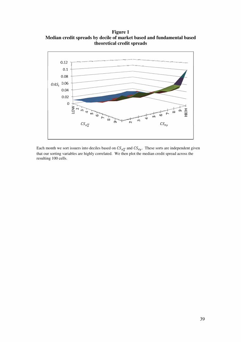
To help visualize the relative importance of component measures of asset

volatility for credit spreads, each month we sort issuers into deciles based on 0,hcz

and 0,hs. These sorts are independent as the two measures of theoretical spreads are

highly correlated (Pearson correlation of 0.93 reported in Panel E of Table 1). We

then plot the median credit spread across the resulting 100 cells. It is clear that as we

move from the back to the front of Figure 1 (that is increasing theoretical spreads

based on market information) we see credit spreads increase. It is also clear that as

we move from left to right of Figure 1 (that is increasing theoretical spreads based on

accounting information) we see also credit spreads increase. What is most interesting,

though, is the increase in credit spreads along the main diagonal: when information

from the market and financial statements are suggesting higher asset volatility then

26

credit spreads are indeed higher. A combination of market and accounting based

measures of asset volatility is superior to either source alone. We find similar patterns

if we instead sort issuers on the basis of 0,hcwz as an alternative market based measure

of theoretical spreads, and either 0,tu1t1 or 0,hsvcwbx as alternative accounting based

measures of theoretical spreads. For the sake of brevity we do not show these figures,

but they are available upon request.

Table 6 reports the results of equation (7) where we allow the regression

coefficients to vary for Investment Grade (IG) and High Yield (HY) issuers. As

before in Table 4, for the sake of brevity we only report the differential coefficients

for HY issuers with respect to the theoretical credit spread measures. In contrast to

the evidence in Table 4, we now find stronger evidence that accounting based

component measures of asset volatility are more relevant to explain cross-sectional

variation in credit spreads for HY issuers relative to IG issuers. This inference is true

for all three theoretical spreads using accounting based component measures of asset

volatility: models (8), (10), and (12) in Table 6 all show a statistically significant

positive coefficient on the respective interaction terms.

3.3 Systematic vs. idiosyncratic volatility

The empirical analysis thus far suggests that combining market and accounting

information generates superior estimates of asset volatility for forecasting bankruptcy

and also for explaining cross-sectional variation in credit spreads. To help better

understand the relative information content of each component measure of asset

volatility we assess the extent to which market and accounting measures of returns are

attributable to systematic versus idiosyncratic factors.

27

As discussed in the introduction, total volatility is the relevant measure of

volatility for explaining derivative prices. This is readily apparent from inspection of

equations (9) and (10). Equation (10) is a contingent claims representation of credit

spreads. Spreads are (i) increasing in the cumulative risk neutral bankruptcy

probability, 0�]l",#B , and (ii) increasing in the expected loss given bankruptcy,

�1 − ",#&. As per equation (9), the primary determinant of 0�]l",#B is the cumulative

physical bankruptcy probability, 02]",#B , which, in turn, is a function of the expected

physical bankruptcy probability, 4�2]"#B& . Equation (8) shows that total asset

volatility is a key determinant of 4�2]"#B&. Thus, estimates of total volatility, and not

just systematic volatility, are relevant for understanding credit spreads. Accordingly,

an association between idiosyncratic equity (Campbell and Taksler, 2003) and bond

(Gemmill and Keswani, 2011) volatility and credit spreads has been documented

empirically at both the issuer and aggregate level.

In addition to total asset volatility, systematic risk is also relevant for

understanding credit spreads. This is because we need to map physical bankruptcy

probabilities to risk neutral bankruptcy probabilities. Equation (9) shows one

approach to do this which assumes a single factor pricing model. More generally,

firm sensitivity to risk and the market price of risk will map physical bankruptcy

probabilities to risk neutral bankruptcy probabilities. Thus, sources of systematic risk

(e.g., correlation of asset returns to aggregate asset returns) represent an additional

source of volatility that will be priced in credit spreads. In credit markets both

systematic and idiosyncratic sources of asset volatility are relevant for determining

credit spreads, and given equations (9) and (10) systematic sources will be relatively

more important (as it affects both asset volatility and the risk premium).

28

It is quite possible that measures of asset volatility extracted from financial

statements capture relatively more idiosyncratic information relative to market based

measures of asset volatility. Market based measures of asset volatility are based on

changes in prices in equity and credit markets, which in turn, are driven by changes in

expectations of cash flows and changes in expectations of discount rates. Arguably,

the latter component is a larger determinant of changes in security prices, especially

as the return interval is shortened (e.g., Richardson, Sloan and Yu, 2012). In contrast,

measures of volatility based on changes in accounting rates of return are a direct

consequence of applying accounting rules to firm transactions over a given fiscal

period. These accounting measures are mostly backward looking in terms of the cash

flow generation and are only indirectly capturing changing expectations of discount

rates (e.g., Penman, Reggiani, Richardson, and Tuna, 2013).

To assess the difference in the mapping of market and accounting based

measures of asset volatility to systematic and idiosyncratic sources, we first examine

the strength of commonality across market and accounting based measures of returns.

We do this by computing pair-wise correlations between market and accounting based

measures of returns for all possible pairs within each Fama-French sector (11 sectors

in total, excluding financials). We estimate these correlations using return measures

over non-overlapping three month intervals, and require at least 20 three month

periods for each pair. For example, if there are 500 issuers in the manufacturing

sector but only 133 issuers have at least twenty three month periods to compute all

three return measures (equity, credit, and accounting), we then compute all 133*132/2

= 8,778 pairs. We end up with fewer than 8,788 pairs, as not all issuers have twenty

non-overlapping three month returns for all three return measures. In Table 7 we

report the resulting average pairwise correlations. In Panel A we average across all

29

industries and in Panel B we report results by industry. In both panels there is a

striking difference in the average pairwise correlation: equity and credit market based

return measures have a much higher average pairwise correlation than accounting

based measures of returns (between 0.38 and 0.46 for market based for the pooled

sample and only 0.09 for accounting based for the pooled sample). This is a

necessary condition for accounting and market based return measures to differentially

reflect systematic and idiosyncratic sources of risk. In unreported tests, we also

identify the first principal component for a balanced panel of 500 issuers that have

non-missing credit, equity and accounting rates of return for our time period. We find

that the first principal component explains 22.7 (35.3) percent of the cross-sectional

variation in equity (credit) returns, but only 13.2 percent for accounting rates of return.

The results in Table 7 suggest that the market based measures are more likely

to reflect systematic sources of volatility. To address more directly the extent to

which market based measures of asset volatility reflect systematic sources more so

than accounting based measures of asset volatility, we perform standard asset pricing

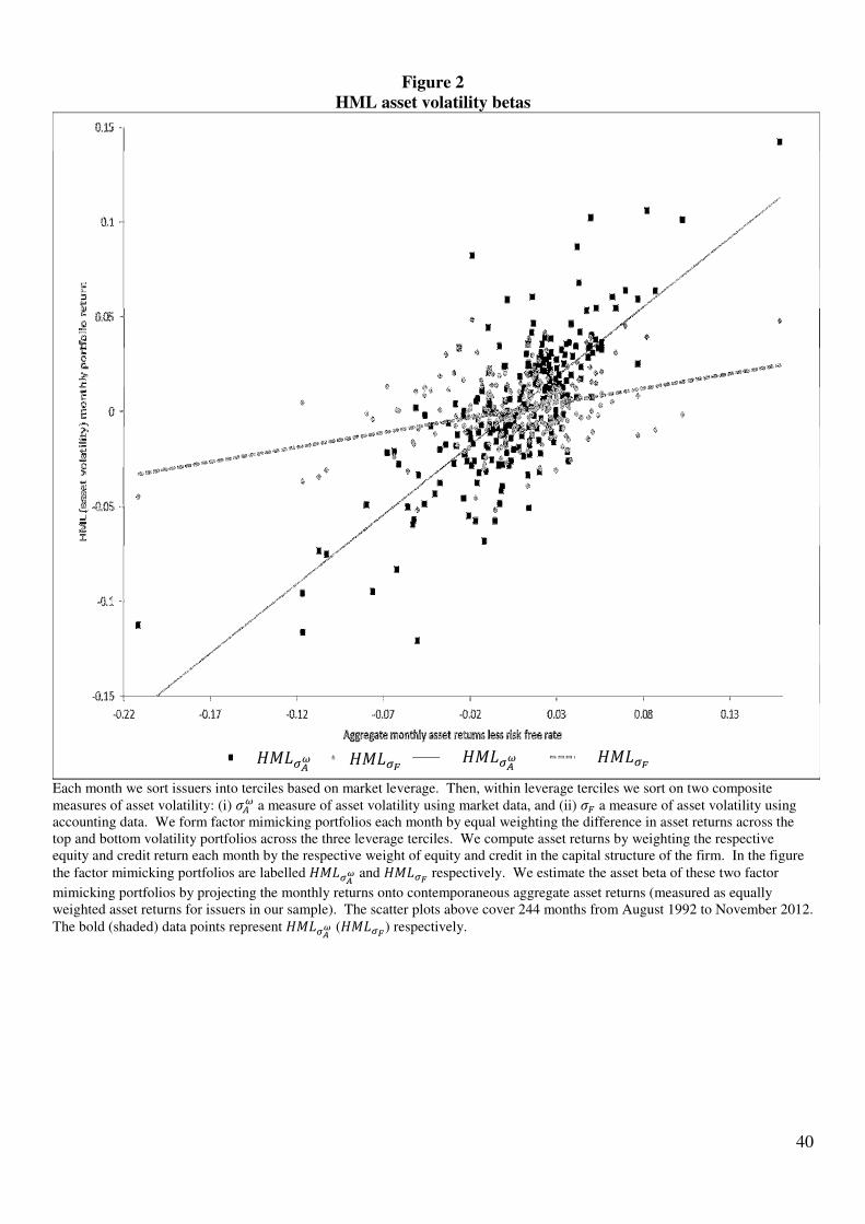
tests. First, we construct multiple factor mimicking portfolios on the basis of our

component measures of asset volatility. For the sake of brevity we only discuss and

tabulate one market based measure, ��, and one accounting based measure, �=, but

results are similar with alternative measures. To abstract away from the effects of

leverage, we first sort issuers each month into terciles on the basis of market leverage.

Then, within each leverage terciles we sort on the two composite measures of asset

volatility, �� and �=, again into terciles. We then form factor mimicking portfolios

each month by equal weighting the difference in asset returns across the top and

bottom volatility portfolios across the three leverage terciles, labelled as ~�+hcz and

~�+hs respectively. We compute asset returns by weighting the respective equity

30

and credit return each month by the respective weight of equity and credit in the

capital structure of the firm. Panel A (B) of Table 8 reports the average annualized

asset returns and associated Sharpe ratios across the 9 cells for the market

(accounting) based component measure of asset volatility. The resulting ~�+hcz and

~�+hs factor mimicking portfolios have similar unconditional Sharpe ratios (about

0.2). We next estimate the asset beta of these two factor mimicking portfolios by

projecting the monthly portfolio asset returns onto contemporaneous aggregate asset

returns (measured as the equally weighted asset returns for issuers in our sample).

The data used for this analysis covers 244 months from August 1992 to November

2012. Figure 2 contains the scatter plots for the two factor mimicking portfolios

along with the respective OLS regression line. The bold (shaded) data points and

lines represent ~�+hcz (~�+hs ) respectively. Tests of difference reveal a strong

difference in asset beta: the asset beta for the ~�+hcz portfolio is 0.73, and the asset

beta for the ~�+hs portfolio is 0.15, test statistic for difference is 11.29 significant at

conventional levels). Results are similar if we instead extract a credit or equity return

beta as opposed to the asset beta that we show in Figure 2.

The evidence in Tables 7 and 8, and Figure 2, show that market based

measures of asset volatility capture relatively more systematic sources of volatility

and accounting based measures of asset volatility capture more idiosyncratic sources

of volatility. This provides a basis for why both market and accounting based

measures were useful in generating estimates of asset volatility for forecasting

bankruptcy and also for explaining cross-sectional variation in credit spreads. Further,

as equations (9) and (10) note, systematic sources of volatility (and hence risk) are

relatively more important as they are relevant for measuring asset volatility (key input

31

to distance to default) and assessing the risk premium to convert risk neutral

bankruptcy probabilities to credit spreads.

3.4 Extensions and robustness tests

3.4.1 CDS data

In Table 9 we report regression estimates of a modified version of equation

(11) where we use credit spreads from CDS contracts rather than bonds. As with our

previous spread level regressions, we include a set of month fixed effects and as such

do not report a regression intercept. A benefit of this approach is that the credit

spread is a cleaner representation of credit risk, but a disadvantage is the shorter time

period for which this data is available (2003 to 2012 only). Because we are

examining cross-sectional variation in 5 year CDS spreads, 0],53# , we no longer

need to control for issue specific characteristics such as �\S# and ]^RZ>[YM#. All 5

year CDS contracts have the same seniority, the same time since issuance (we only

examine ‘on the run’ contracts), and the same tenor (5 years). Thus, we estimate the

following model:

0],53# = V)4QRS># + V LM(4#) + ∑ VB� WBG) 0,hr,O + X0YM>RYL# + F# (12)

Our sample size decreases from 55,431 bond-months examined in Table 5 to

29,557 CDS-months examined in Table 9. Despite the smaller sample size, we find

striking results with this alternative sample. Models (1) to (4) show that theoretical

spreads based on equity market information are able to explain up to 53.6 percent of

the cross-sectional variation in credit spreads. Models (5) and (6) show that by

combining component measures of asset volatility generates theoretical spreads that

can explain a greater fraction of the cross-sectional variation in credit spreads (the R2

increases to 65.3 percent for model (6)). Strikingly, our measure of theoretical spread

using fundamental volatility alone can explain 64.1 percent of the cross-sectional

32

variation in credit spreads (see model (7)). Finally, including both market and

accounting based measures of asset volatility yields theoretical spreads that can

explain even more of the cross-sectional variation in credit spreads: R2 of 69.5 percent

in models (8) and (10). Similar to the analysis in Table 5, at the bottom of Table 9 we

also report the R2 of the equivalent unconstrained regression on the CDS sample.

Across all of the specifications, with the exception of model (1), we see statistically

significant increases in explanatory power when we constrain asset volatility and

leverage, consistent with the Merton model, as compared to including these variables

linearly and independently.

3.4.2 Alternative specifications

In untabulated analysis, we expand the bankruptcy forecasting model to

control for average accounting profitability over the previous four quarters, cash

holdings, market to book ratio and price, following Campbell, Hilscher and Szilagyi

(2008). We choose not include these variables in our main specification, which only

includes (albeit linearly), the main determinants of probability of default as per the

Merton model. Specifically, we add the following variables to the analysis reported

in Table 3 (variables are defined and labelled consistently with Campbell, Hilscher

and Szilagyi, 2008): (i) NIMTAAVG, a geometrically weighted average level of net

income scaled by market value of total assets, which places higher weight on more

recent quarters, (ii) CASHMTA, cash and short term investments scaled by the market

value of assets, (iii) MB, the market to book ratio, and (iv) PRICE the natural

logarithm of the firm’s stock price. The sample size does not change significantly as

a result of the inclusion of these additional control variables (reduced from 67,373

bond-month to 67,124 bond-month observations). Our measures of fundamental

33

volatility continue to be significant, both when included individually and together

with implied volatility and debt volatility.

We also re-estimate the unconstrained and constrained credit spread

regressions adding the control variables in Campbell and Taskler (2003). In particular,

we control for operating income and long term debt to total assets. The sample size

for the unconstrained analysis is reduced from 67,117 to 62,146 bond-month

observations. Consistent with our main analysis, we continue to find that fundamental

volatility is significant both when included individually and when considered

incrementally to debt volatility and implied volatility. Similarly, in the constrained

analysis, credit spreads based on fundamental volatility remain both individually and

incrementally significant.

4. Conclusion

In this paper we evaluate alternative measures of asset volatility using

information from (i) historical security returns (both equity and credit), (ii) implied

volatilities extracted from equity options, and (iii) financial statements. We find that

combining component measures of asset volatility across these three sources

generates superior forecasts of bankruptcy, and in turn, is better able to explain cross-

sectional variation in corporate bond and corporate CDS spreads for a large sample of

US corporate issuers.

We further show that market based component measures of asset volatility

have a greater common component to them as evidenced by greater pairwise

correlations between market based measures of returns relative to accounting based

measures of returns. This greater comovement of market based measures of returns is

strongly evident in differential asset betas of factor mimicking portfolios generated on

34

the basis of market versus accounting based component measures of asset volatility.

The market based asset volatility factor mimicking portfolio has a much larger beta to

aggregate market returns, suggesting that market based measures reflect systematic

sources of volatility and accounting based measures reflect idiosyncratic sources of

volatility. Thus, combining market and accounting based measures of asset volatility

generates a superior measure of total asset volatility that is relevant for understanding

credit spreads.

35

References

Arora, N., J. Bohn and F. Zhu (2005). Reduced form vs. structural models of credit risk: a

case study of 3 models. Journal of Investment Management 3 (4): 43-67.

Beaver, W.H., M. Correia and M. McNichols (2012). Do differences in financial

reporting attributes impair the predictive ability of financial ratios for bankruptcy.

Review of Accounting Studies 17 (4): 969-1010.

Beaver, W. H., M. McNichols, and J. Rhie (2005). Have financial statements become

less informative? Evidence from the ability of financial ratios to predict bankruptcy.

Review of Accounting Studies 10: 93-122.

Bharath, S. and T. Shumway (2008). Forecasting default with the Merton distance to

default model. Review of Financial Studies 21: 1339-1369.

Bruche, M., C. Gonzales-Aguado (2009). Recovery rates, default probabilities, and

the credit cycle. CEMFI Working Paper.

Campbell, J. and G. Taksler (2003). Equity volatility and corporate bond yields. The

Journal of Finance 58 (6): 2321-2349.

Cao, C., F. Yu and Z. Zhong (2010). The information content of option-implied

volatility for credit default swap valuation. Journal of Financial Markets 13: 321-343.

Chang, W., S. Monahan and A. Ouazad (2013). The Higher Moments of Future

Return on Equity. Working Paper.

Chava, S., and R. Jarrow (2004). Bankruptcy prediction with industry effects. Review

of Finance 8: 537-569.

Correia, M., S. Richardson and I. Tuna (2012). Value Investing in Credit Markets.

Review of Accounting Studies 17 (3): 572-609.

Cremers, M., J. Driessen, P. Maenhout and D. Weinbaum (2008). Individual stock-

option prices and credit spreads. Journal of Banking & Finance 32(12): 2706-2715.

Crouhy, M, D. Galai and R. Mark (2000). A comparative analysis of current

credit risk models. Journal of Banking & Finance 24: 59-117.

Fama, E., and K. French (2000). Forecasting profitability and earnings. Journal of

Business 72: 161–175.

Gemmill, G. and A. Keswani (2011). Downside risk and the size of credit spreads.

Journal of Banking and Finance 35 (8): 2021-2036.

Goodman, T., M. Neamtiu and F. Zhang. (2012). Fundamental Analysis and Option

Returns. Working Paper. http://papers.ssrn.com/sol3/papers.cfm?abstract_id=1974753

36

Haesen D. P. Howeling and V. Van Zundert (2012). Equity Momentum for Corporate

Bonds: Identifying, Understanding and Reducing Time-Varying Factor Exposures.

Working Paper. http://papers.ssrn.com/sol3/papers.cfm?abstract_id=2131032

Helwege, J., and C. M. Turner (1999). The slope of the credit yield curve for

speculative grade issuers. Journal of Finance, 54, 1869-1884.

Kealhoffer, S.( 2003). Quantifying Credit Risk II: Debt Valuation. Financial Analysts

Journal, May/June: 78-92.

Konstantinidi, T. and P. Pope (2012). Forecasting Risk in Earnings. Working paper.

http://papers.ssrn.com/sol3/papers.cfm?abstract_id=1903378.

Hou, K., M.A. Van Dijk and Y. Zhang (2012). The Implied Cost of Capital: A New

Approach. Journal of Accounting and Economics 53(3): 504-526.

Lok, S. and S. Richardson (2011). Credit markets and financial information. Review

of Accounting Studies 16: 487-500.

Merton, R. (1974). On the pricing of corporate debt: The risk structure of interest

rates. Journal of Finance 29: 449-470.

Penman, S. H. (1991). An Evaluation of Accounting Rate-of-Return. Journal of

Accounting, Auditing and Finance Spring: 233-255.

Penman, S.H., F. Reggiani, S. A. Richardson and I. Tuna (2013). An

accounting’based characteristic model for asset pricing. Working paper.

http://papers.ssrn.com/sol3/papers.cfm?abstract_id=1966566

Richardson, S. A., R. G. Sloan, M. T. Soliman and I. Tuna (2006). The implications

of accounting distortions and growth for accruals and profitability. The Accounting

Review 81(3): 713-743.

Richardson, S.A., R.G. Sloan and H. You (2012). What makes stock prices move?

Fundamental vs. investor recognition. Financial Analysts Journal 68(2)

Schaefer, S. and I. Strebulaev (2008). Structural models of credit risk are useful: evidence

from hedge ratios on corporate bonds. Journal of Financial Economics: 1-19.

Shumway, T. (2001). Forecasting bankruptcy more accurately: A simple hazard

model. Journal of Business 74: 101-124.

Sloan, R. G. (1996). Do stock prices fully reflect information in accruals and cash flows

about future earnings?. The Accounting Review 81 (3): 289-315.

Sridharan, S. (2012) Volatility Forecasting using Fundamental Information. Working

Paper. http://papers.ssrn.com/sol3/papers.cfm?abstract_id=1984324

Vuolteenaho, T. (2002) What drives firm-level stock returns? The Journal of Finance

57(1): 233-264.

37

Appendix: Variable Definitions

Compustat mnemonics in parenthesis

Panel A: Volatility Measures

Variable Description �� Historical equity volatility, the annualized standard deviation of

realized daily stock returns over the previous 252 days. �� Implied volatility, the average of implied Black and Scholes

volatility estimates for at-the-money 91-day call and put options

(source: Option Metrics Iv DB standardized database). �� Debt volatility, the standard deviation of total monthly bond returns,

computed over the previous 12 months (computed based on Barcap

total return). ������� Naively deleveraged historical equity volatility, �� ���.

��� Weighted historical volatility, �� �� + (1 − �) �� + 2��,�����. �������� Naively deleveraged implied equity volatility, �� ���. ���� Weighted implied volatility, �� �� + (1 − �) �� + 2��,�����. �= Fundamental volatility, the standard deviation of the estimated

RNOA percentiles (RNOA is computed for each quarter as the

rolling sum of ‘OIADP’ for the previous 4 quarters, scaled by the

average of the opening and ending balance of NOA over this 4

quarter period). 29525 The difference between the estimated 95th

and 5th

percentiles of the

RNOA distribution. �=����� The standard deviation of the difference between quarterly RNOA

and RNOA for the same quarter of the previous year, computed over

the previous 5 years (requiring a minimum of 10 quarters of data).

Panel B: Credit spreads and other variables used in the estimation of asset volatility

and theoretical credit spreads

Variable Description !�, Option adjusted spread (source: Barcap). !�] Option adjusted duration (source: Barcap). ; Book value of short term debt (‘DLCC’)+0.5* book value of long term debt

(‘DLTTQ’). 4 Market capitalization, calculated as |‘PRC’|*’SHROUT’ (source: CRSP

monthly file). � ��� , the ratio of market capitalization and the sum of market capitalization

and the book value of debt. 2

,tir Correlation between the firm’s monthly equity return and the market value

weighted return calculated over the prior 5 years (computed based on the

CRSP monthly file).

38

��,� Average correlation of monthly equity and bond returns, calculated over the

prior 12 months for all bonds in the same decile of OAS (computed based

on the equity returns from the CRSP monthly file and total bond returns

from Barcap).

Panel C: Fundamental volatility estimation

Variable Description

RNOA Return on net operating assets, defined as the ratio of operating

income after depreciation (‘OIADP’) and the average of the

opening and closing balance of net operating assets (NOA).

NOA Net operating assets, defined as the sum of common equity,

preferred stock, long-term debt, debt in current liabilities and

minority interests minus cash and short term investments,

‘CEQ’+’PSTK’+’DLTT’+’DLC’+’MIB’-‘CHE’.

Accruals Accruals scaled by the average of the opening and closing balance

of NOA, with accruals calculated as ∆’ACT’-∆‘CHE’-(∆’LCT’-

∆’DLC’- ∆ ‘TXP’)-‘DP’, where ‘ACT’ are current assets, ‘CHE’

cash and short term investments, ‘LCT’ current liabilities, ‘DLC’

debt in current liabilities, ‘TXP’ taxes payable and ‘DP’

depreciation and amortization.

Loss An indicator variable equal to 1 if RNOA<0, 0 otherwise.

Payer An indicator variable equal to 1 if Payout>0, 0 otherwise.

Payout Dividends paid, ‘DVPSX_F’, scaled by the average opening and

closing balances of RNOA.

Panel D: Credit Spreads

Variable Description 0,hx{�C� 0,hx{�C� = − )k �1 − (1 − )0�]l� , where 0�]l = �n�*)(02]) + p√R √�o and 02] = 1 − (1 − 2])k

and PD is the empirically fitted physical probability of default,

resulting from the estimation of the following logistic regression

4(2]) = J�`abcf ���*�x�� �#hx√# �.

0,h�

Similar to 0,hx{�C�, except that 4(2]) = J�`abcc�Of ���*�r�� �#hr√# �, where

U��`# = 4 + ()�|�C)} and �B are the different measures of volatility

described in Panel A.

39

Figure 1

Median credit spreads by decile of market based and fundamental based

theoretical credit spreads

Each month we sort issuers into deciles based on 0,hcz and 0,hs . These sorts are independent given

that our sorting variables are highly correlated. We then plot the median credit spread across the

resulting 100 cells.

0,hcz 0,hs

!�,#

40

Figure 2

HML asset volatility betas

Each month we sort issuers into terciles based on market leverage. Then, within leverage terciles we sort on two composite

measures of asset volatility: (i) �� a measure of asset volatility using market data, and (ii) �= a measure of asset volatility using

accounting data. We form factor mimicking portfolios each month by equal weighting the difference in asset returns across the

top and bottom volatility portfolios across the three leverage terciles. We compute asset returns by weighting the respective

equity and credit return each month by the respective weight of equity and credit in the capital structure of the firm. In the figure

the factor mimicking portfolios are labelled ~�+hcz and ~�+hs respectively. We estimate the asset beta of these two factor

mimicking portfolios by projecting the monthly returns onto contemporaneous aggregate asset returns (measured as equally

weighted asset returns for issuers in our sample). The scatter plots above cover 244 months from August 1992 to November 2012.

The bold (shaded) data points represent ~�+hcz (~�+hs) respectively.

~�+hcz ~�+hs ~�+hs ~�+hcz

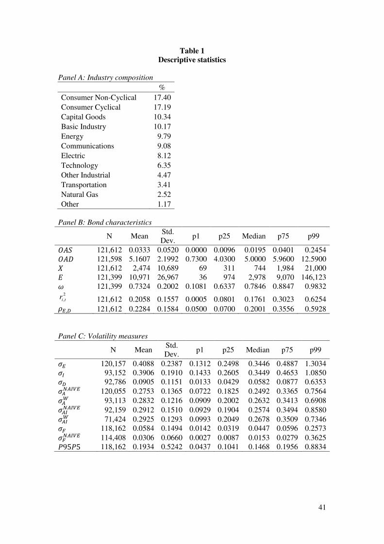
41

Table 1

Descriptive statistics

Panel A: Industry composition

%

Consumer Non-Cyclical 17.40

Consumer Cyclical 17.19

Capital Goods 10.34

Basic Industry 10.17

Energy 9.79

Communications 9.08

Electric 8.12

Technology 6.35

Other Industrial 4.47

Transportation 3.41

Natural Gas 2.52

Other 1.17

Panel B: Bond characteristics

N Mean

Std.

Dev. p1 p25 Median p75 p99 !�, 121,612 0.0333 0.0520 0.0000 0.0096 0.0195 0.0401 0.2454 !�] 121,598 5.1607 2.1992 0.7300 4.0300 5.0000 5.9600 12.5900 ; 121,612 2,474 10,689 69 311 744 1,984 21,000 4 121,399 10,971 26,967 36 974 2,978 9,070 146,123 � 121,399 0.7324 0.2002 0.1081 0.6337 0.7846 0.8847 0.9832

2

,tir 121,612 0.2058 0.1557 0.0005 0.0801 0.1761 0.3023 0.6254 ��,� 121,612 0.2284 0.1584 0.0500 0.0700 0.2001 0.3556 0.5928

Panel C: Volatility measures

N Mean Std.

Dev. p1 p25 Median p75 p99 �� 120,157 0.4088 0.2387 0.1312 0.2498 0.3446 0.4887 1.3034 �� 93,152 0.3906 0.1910 0.1433 0.2605 0.3449 0.4653 1.0850 �� 92,786 0.0905 0.1151 0.0133 0.0429 0.0582 0.0877 0.6353 ������� 120,055 0.2753 0.1365 0.0722 0.1825 0.2492 0.3365 0.7564 ��� 93,113 0.2832 0.1216 0.0909 0.2002 0.2632 0.3413 0.6908 �������� 92,159 0.2912 0.1510 0.0929 0.1904 0.2574 0.3494 0.8580 ���� 71,424 0.2925 0.1293 0.0993 0.2049 0.2678 0.3509 0.7346 �= 118,162 0.0584 0.1494 0.0142 0.0319 0.0447 0.0596 0.2573 �=����� 114,408 0.0306 0.0660 0.0027 0.0087 0.0153 0.0279 0.3625 29525 118,162 0.1934 0.5242 0.0437 0.1041 0.1468 0.1956 0.8834

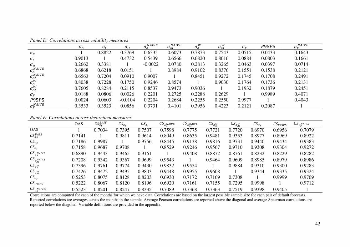
42

Panel D: Correlations across volatility measures

�� �� �� ������� �������� ��� ���� �= 29525 �=����� �� 1 0.8822 0.3769 0.6335 0.6073 0.7873 0.7543 0.0515 0.0433 0.1643 �� 0.9013 1 0.4732 0.5439 0.6566 0.6820 0.8016 0.0884 0.0803 0.1661 �� 0.2662 0.3381 1 -0.0022 0.0780 0.2813 0.3265 0.0463 0.0397 0.0714 ������� 0.6868 0.6218 0.0151 1 0.8984 0.9102 0.8376 0.1551 0.1538 0.2121 �������� 0.6563 0.7204 0.0910 0.9007 1 0.8451 0.9272 0.1745 0.1708 0.2491 ��� 0.8038 0.7228 0.1750 0.9246 0.8574 1 0.9030 0.1764 0.1736 0.2131 ���� 0.7605 0.8284 0.2115 0.8537 0.9473 0.9036 1 0.1932 0.1879 0.2451 �= 0.0188 0.0806 0.0026 0.2201 0.2725 0.2288 0.2629 1 0.9989 0.4071 29525 0.0024 0.0603 -0.0104 0.2204 0.2684 0.2255 0.2550 0.9977 1 0.4043 �=����� 0.3533 0.3523 0.0856 0.3731 0.4101 0.3956 0.4223 0.2121 0.2087 1

Panel E: Correlations across theoretical measures

OAS 0,hx{�C� 0,hx 0,hd 0,hcvcwbx 0,hcdvcwbx 0,hcz 0,hcwz 0,hs 0,tu1t1 0,hsvcwbx

OAS 1 0.7034 0.7395 0.7507 0.7598 0.7775 0.7721 0.7720 0.6970 0.6956 0.7079 0,hx{�C� 0.7141 1 0.9811 0.9614 0.8049 0.8635 0.9481 0.9353 0.8977 0.8969 0.8922 0,hx 0.7186 0.9987 1 0.9756 0.8445 0.9138 0.9816 0.9731 0.9440 0.9434 0.9383 0,hd 0.7158 0.9687 0.9708 1 0.8529 0.9246 0.9567 0.9710 0.9308 0.9304 0.9272 0,hcvcwbx 0.6890 0.9443 0.9465 0.9161 1 0.9408 0.8872 0.8761 0.8232 0.8229 0.8282 0,hcdvcwbx 0.7208 0.9342 0.9367 0.9699 0.9543 1 0.9464 0.9609 0.8985 0.8979 0.8986 0,hcz 0.7396 0.9761 0.9774 0.9430 0.9832 0.9554 1 0.9884 0.9310 0.9300 0.9283 0,hcwz 0.7426 0.9472 0.9495 0.9803 0.9448 0.9955 0.9608 1 0.9344 0.9335 0.9324 0,hs 0.5253 0.8075 0.8128 0.8203 0.6930 0.7172 0.7169 0.7308 1 0.9999 0.9709 0,tu1t1 0.5222 0.8067 0.8120 0.8196 0.6920 0.7161 0.7155 0.7295 0.9998 1 0.9712 0,hsvcwbx, 0.5523 0.8201 0.8247 0.8335 0.7089 0.7368 0.7363 0.7519 0.9398 0.9405 1 Correlations are computed for each of the months for which we have data. Correlations are based on the largest possible sample size for each pair of default forecasts.

Reported correlations are averages across the months in the sample. Average Pearson correlations are reported above the diagonal and average Spearman correlations are

reported below the diagonal. Variable definitions are provided in the appendix.

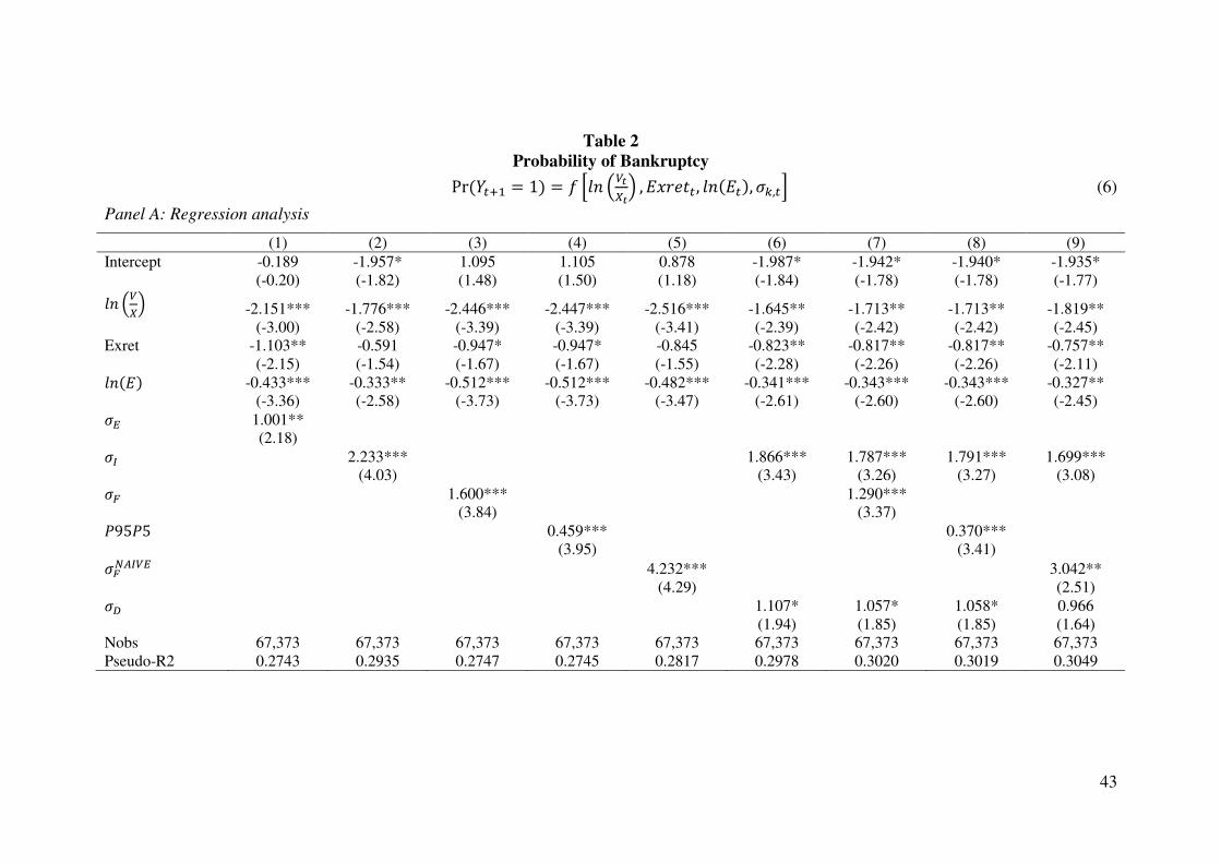
43

Table 2

Probability of Bankruptcy Pr(3#�) = 1) = J KLM N�OOP , 4QRS>#, LM(4#), �B,#T (6)

Panel A: Regression analysis

(1) (2) (3) (4) (5) (6) (7) (8) (9)

Intercept -0.189 -1.957* 1.095 1.105 0.878 -1.987* -1.942* -1.940* -1.935*

(-0.20) (-1.82) (1.48) (1.50) (1.18) (-1.84) (-1.78) (-1.78) (-1.77) LM N�P -2.151*** -1.776*** -2.446*** -2.447*** -2.516*** -1.645** -1.713** -1.713** -1.819**

(-3.00) (-2.58) (-3.39) (-3.39) (-3.41) (-2.39) (-2.42) (-2.42) (-2.45)

Exret -1.103** -0.591 -0.947* -0.947* -0.845 -0.823** -0.817** -0.817** -0.757**

(-2.15) (-1.54) (-1.67) (-1.67) (-1.55) (-2.28) (-2.26) (-2.26) (-2.11) LM(4) -0.433*** -0.333** -0.512*** -0.512*** -0.482*** -0.341*** -0.343*** -0.343*** -0.327**

(-3.36) (-2.58) (-3.73) (-3.73) (-3.47) (-2.61) (-2.60) (-2.60) (-2.45) �� 1.001**

(2.18) �� 2.233*** 1.866*** 1.787*** 1.791*** 1.699***

(4.03) (3.43) (3.26) (3.27) (3.08) �= 1.600*** 1.290***

(3.84) (3.37) 29525 0.459*** 0.370***

(3.95) (3.41) �=����� 4.232*** 3.042**

(4.29) (2.51) �� 1.107* 1.057* 1.058* 0.966

(1.94) (1.85) (1.85) (1.64)

Nobs 67,373 67,373 67,373 67,373 67,373 67,373 67,373 67,373 67,373

Pseudo-R2 0.2743 0.2935 0.2747 0.2745 0.2817 0.2978 0.3020 0.3019 0.3049

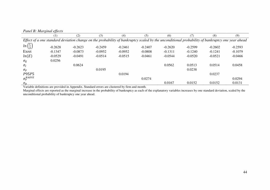
44

Panel B: Marginal effects

(1) (2) (3) (4) (5) (6) (7) (8) (9)

Effect of a one standard deviation change on the probability of bankruptcy scaled by the unconditional probability of bankruptcy one year ahead LM N�P -0.2628 -0.2623 -0.2459 -0.2461 -0.2407 -0.2620 -0.2599 -0.2602 -0.2593

Exret -0.1347 -0.0873 -0.0952 -0.0952 -0.0808 -0.1311 -0.1240 -0.1241 -0.1079 LM(4) -0.0529 -0.0491 -0.0514 -0.0515 -0.0461 -0.0544 -0.0520 -0.0521 -0.0466 �� 0.0256 �� 0.0624 0.0562 0.0513 0.0514 0.0458 �= 0.0195 0.0238 29525 0.0194 0.0237 �=����� 0.0274 0.0294 �� 0.0167 0.0152 0.0152 0.0131 Variable definitions are provided in Appendix. Standard errors are clustered by firm and month.

Marginal effects are reported as the marginal increase in the probability of bankruptcy as each of the explanatory variables increases by one standard deviation, scaled by the

unconditional probability of bankruptcy one year ahead.

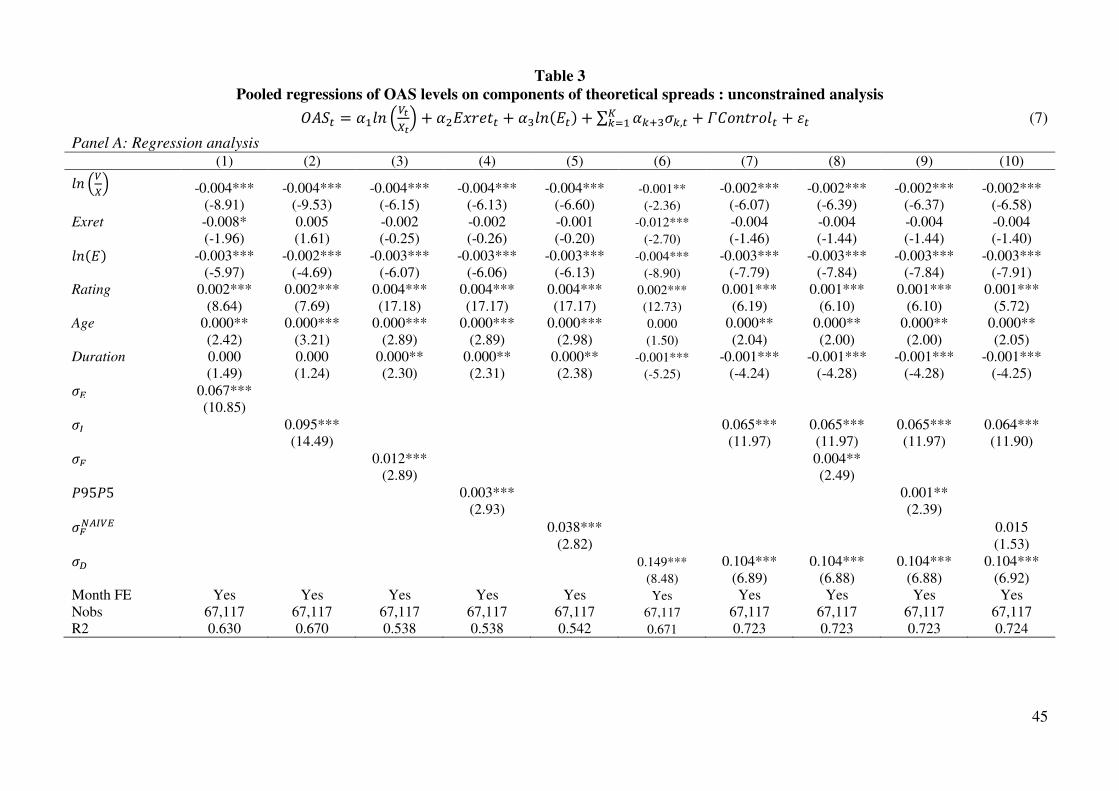
45

Table 3

Pooled regressions of OAS levels on components of theoretical spreads : unconstrained analysis !�,# = V)LM N�OOP + V 4QRS># + V-LM(4#) + ∑ VB�-�B,#WBG) + X0YM>RYL# + F# (7)

Panel A: Regression analysis

(1) (2) (3) (4) (5) (6) (7) (8) (9) (10) LM N�P -0.004*** -0.004*** -0.004*** -0.004*** -0.004*** -0.001** -0.002*** -0.002*** -0.002*** -0.002***

(-8.91) (-9.53) (-6.15) (-6.13) (-6.60) (-2.36) (-6.07) (-6.39) (-6.37) (-6.58)

Exret -0.008* 0.005 -0.002 -0.002 -0.001 -0.012*** -0.004 -0.004 -0.004 -0.004

(-1.96) (1.61) (-0.25) (-0.26) (-0.20) (-2.70) (-1.46) (-1.44) (-1.44) (-1.40) LM(4) -0.003*** -0.002*** -0.003*** -0.003*** -0.003*** -0.004*** -0.003*** -0.003*** -0.003*** -0.003***

(-5.97) (-4.69) (-6.07) (-6.06) (-6.13) (-8.90) (-7.79) (-7.84) (-7.84) (-7.91)

Rating 0.002*** 0.002*** 0.004*** 0.004*** 0.004*** 0.002*** 0.001*** 0.001*** 0.001*** 0.001***

(8.64) (7.69) (17.18) (17.17) (17.17) (12.73) (6.19) (6.10) (6.10) (5.72)

Age 0.000** 0.000*** 0.000*** 0.000*** 0.000*** 0.000 0.000** 0.000** 0.000** 0.000**

(2.42) (3.21) (2.89) (2.89) (2.98) (1.50) (2.04) (2.00) (2.00) (2.05)

Duration 0.000 0.000 0.000** 0.000** 0.000** -0.001*** -0.001*** -0.001*** -0.001*** -0.001***

(1.49) (1.24) (2.30) (2.31) (2.38) (-5.25) (-4.24) (-4.28) (-4.28) (-4.25) �� 0.067***

(10.85) �� 0.095*** 0.065*** 0.065*** 0.065*** 0.064***

(14.49) (11.97) (11.97) (11.97) (11.90) �= 0.012*** 0.004**

(2.89) (2.49) 29525 0.003*** 0.001**

(2.93) (2.39) �=����� 0.038*** 0.015

(2.82) (1.53) �� 0.149*** 0.104*** 0.104*** 0.104*** 0.104***

(8.48) (6.89) (6.88) (6.88) (6.92)

Month FE Yes Yes Yes Yes Yes Yes Yes Yes Yes Yes

Nobs 67,117 67,117 67,117 67,117 67,117 67,117 67,117 67,117 67,117 67,117

R2 0.630 0.670 0.538 0.538 0.542 0.671 0.723 0.723 0.723 0.724

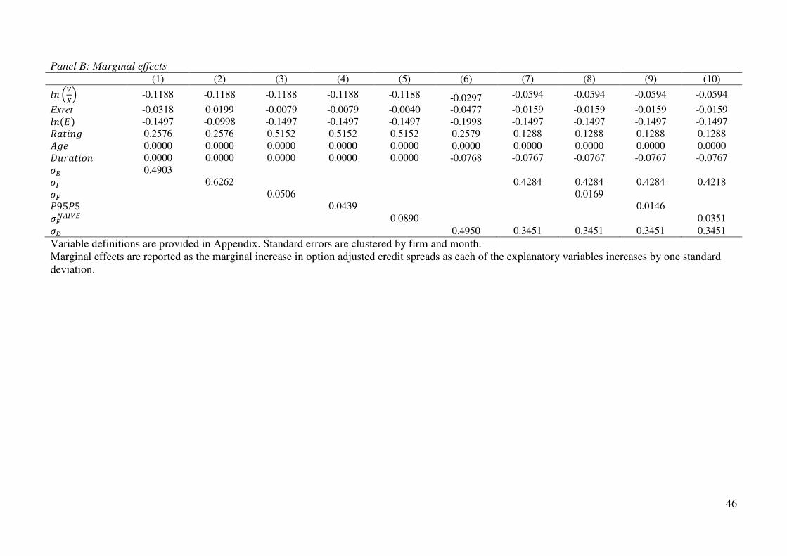
46

Panel B: Marginal effects

(1) (2) (3) (4) (5) (6) (7) (8) (9) (10) LM N�P -0.1188 -0.1188 -0.1188 -0.1188 -0.1188 -0.0297 -0.0594 -0.0594 -0.0594 -0.0594

Exret -0.0318 0.0199 -0.0079 -0.0079 -0.0040 -0.0477 -0.0159 -0.0159 -0.0159 -0.0159 LM(4) -0.1497 -0.0998 -0.1497 -0.1497 -0.1497 -0.1998 -0.1497 -0.1497 -0.1497 -0.1497 Z>[M\ 0.2576 0.2576 0.5152 0.5152 0.5152 0.2579 0.1288 0.1288 0.1288 0.1288 �\S 0.0000 0.0000 0.0000 0.0000 0.0000 0.0000 0.0000 0.0000 0.0000 0.0000 ]^RZ>[YM 0.0000 0.0000 0.0000 0.0000 0.0000 -0.0768 -0.0767 -0.0767 -0.0767 -0.0767 �� 0.4903 �� 0.6262 0.4284 0.4284 0.4284 0.4218 �= 0.0506 0.0169 29525 0.0439 0.0146 �=����� 0.0890 0.0351 �� 0.4950 0.3451 0.3451 0.3451 0.3451

Variable definitions are provided in Appendix. Standard errors are clustered by firm and month.

Marginal effects are reported as the marginal increase in option adjusted credit spreads as each of the explanatory variables increases by one standard

deviation.

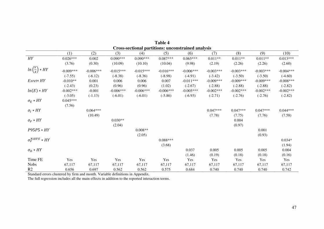
47

Table 4

Cross-sectional partitions: unconstrained analysis (1) (2) (3) (4) (5) (6) (7) (8) (9) (10) ~3 0.026*** 0.002 0.090*** 0.090*** 0.087*** 0.065*** 0.011** 0.011** 0.011** 0.013***

(3.76) (0.30) (10.09) (10.10) (10.04) (9.98) (2.19) (2.26) (2.26) (2.60) LM N�P ∗ ~3 -0.009*** -0.006*** -0.015*** -0.015*** -0.016*** -0.006*** -0.003*** -0.003*** -0.003*** -0.004***

(-7.55) (-6.12) (-8.38) (-8.36) (-8.98) (-4.91) (-3.42) (-3.50) (-3.50) (-4.60)

Exret∗ ~3 -0.010** 0.001 0.006 0.006 0.007 -0.011*** -0.009*** -0.009*** -0.009*** -0.008***

(-2.43) (0.23) (0.96) (0.96) (1.02) (-2.67) (-2.88) (-2.88) (-2.88) (-2.82) LM(4) ∗ ~3 -0.002*** -0.001 -0.006*** -0.006*** -0.006*** -0.005*** -0.002*** -0.002*** -0.002*** -0.002***

(-3.05) (-1.13) (-6.01) (-6.01) (-5.86) (-6.93) (-2.71) (-2.76) (-2.76) (-2.82) �� ∗ ~3 0.045***

(7.56) �� ∗ ~3 0.064*** 0.047*** 0.047*** 0.047*** 0.044***

(10.49) (7.78) (7.75) (7.76) (7.58) �= ∗ ~3 0.030** 0.004

(2.04) (0.97) 29525 ∗ ~3 0.008** 0.001

(2.05) (0.93) �=����� ∗ ~3 0.088*** 0.034*

(3.68) (1.94) �� ∗ ~3 0.037 0.005 0.005 0.005 0.004

(1.46) (0.19) (0.18) (0.18) (0.16)

Time FE Yes Yes Yes Yes Yes Yes Yes Yes Yes Yes

Nobs 67,117 67,117 67,117 67,117 67,117 67,117 67,117 67,117 67,117 67,117

R2 0.656 0.697 0.562 0.562 0.575 0.684 0.740 0.740 0.740 0.742

Standard errors clustered by firm and month. Variable definitions in Appendix.

The full regression includes all the main effects in addition to the reported interaction terms.

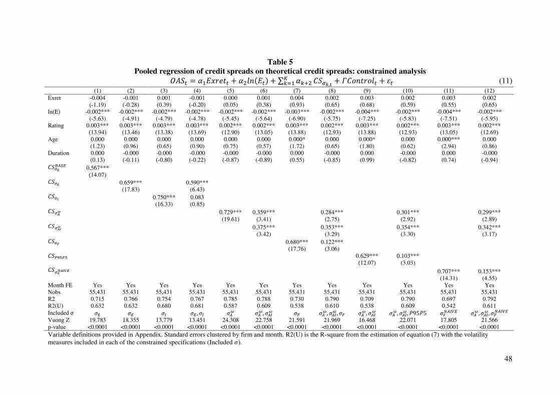
48

Table 5

Pooled regression of credit spreads on theoretical credit spreads: constrained analysis !�,# = V)4QRS># + V LM(4#) + ∑ VB� WBG) 0,hr,O + X0YM>RYL# + F# (11)

(1) (2) (3) (4) (5) (6) (7) (8) (9) (10) (11) (12)

Exret -0.004 -0.001 0.001 -0.001 0.000 0.001 0.004 0.002 0.003 0.002 0.003 0.002

(-1.19) (-0.28) (0.39) (-0.20) (0.05) (0.38) (0.93) (0.65) (0.68) (0.59) (0.55) (0.65)

ln(E) -0.002*** -0.002*** -0.002*** -0.002*** -0.002*** -0.002*** -0.003*** -0.002*** -0.004*** -0.002*** -0.004*** -0.002***

(-5.63) (-4.91) (-4.79) (-4.78) (-5.45) (-5.64) (-6.90) (-5.75) (-7.25) (-5.83) (-7.51) (-5.95)

Rating 0.003*** 0.003*** 0.003*** 0.003*** 0.002*** 0.002*** 0.003*** 0.002*** 0.003*** 0.002*** 0.003*** 0.002***

(13.94) (13.46) (13.38) (13.69) (12.90) (13.05) (13.88) (12.93) (13.88) (12.93) (13.05) (12.69)

Age 0.000 0.000 0.000 0.000 0.000 0.000 0.000* 0.000 0.000* 0.000 0.000*** 0.000

(1.23) (0.96) (0.65) (0.90) (0.75) (0.57) (1.72) (0.65) (1.80) (0.62) (2.94) (0.86)

Duration 0.000 -0.000 -0.000 -0.000 -0.000 -0.000 0.000 -0.000 0.000 -0.000 0.000 -0.000

(0.13) (-0.11) (-0.80) (-0.22) (-0.87) (-0.89) (0.55) (-0.85) (0.99) (-0.82) (0.74) (-0.94) 0,hx{�C� 0.567***

(14.07) 0,hx 0.659*** 0.590***

(17.83) (6.43) 0,hw 0.750*** 0.083

(16.33) (0.85) 0,hcz 0.729*** 0.359*** 0.284*** 0.301*** 0.299***

(19.61) (3.41) (2.75) (2.92) (2.89) 0,hcwz 0.375*** 0.353*** 0.354*** 0.342***

(3.42) (3.29) (3.30) (3.17) 0,hs 0.680*** 0.122***

(17.76) (3.06) 0,tu1t1 0.629*** 0.103***

(12.07) (3.03) 0,hsvcwbx 0.707*** 0.153***

(14.31) (4.55)

Month FE Yes Yes Yes Yes Yes Yes Yes Yes Yes Yes Yes Yes

Nobs 55,431 55,431 55,431 55,431 55,431 55,431 55,431 55,431 55,431 55,431 55,431 55,431

R2 0.715 0.766 0.754 0.767 0.785 0.788 0.730 0.790 0.709 0.790 0.697 0.792

R2(U) 0.632 0.632 0.680 0.681 0.587 0.609 0.538 0.610 0.538 0.609 0.542 0.611

Included � �� �� �� �� , �� �� ��, ��� �= ��, ���, �= ��, ��� ��, ���, 29525 �=����� ��, ���, �=�����

Vuong Z 19.783 18.355 13.779 13.451 24.308 22.758 21.591 21.969 16.468 22.071 17.805 21.566

p-value <0.0001 <0.0001 <0.0001 <0.0001 <0.0001 <0.0001 <0.0001 <0.0001 <0.0001 <0.0001 <0.0001 <0.0001

Variable definitions provided in Appendix. Standard errors clustered by firm and month. R2(U) is the R-square from the estimation of equation (7) with the volatility

measures included in each of the constrained specifications (Included �).

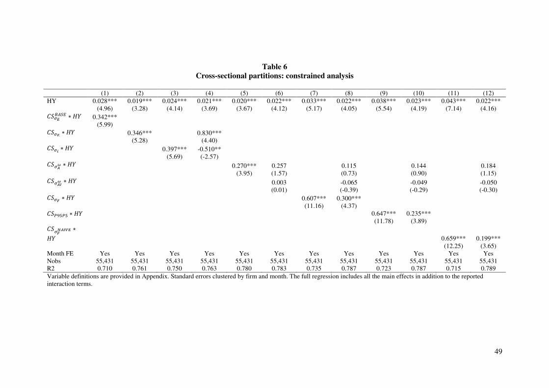
49

Table 6

Cross-sectional partitions: constrained analysis

(1) (2) (3) (4) (5) (6) (7) (8) (9) (10) (11) (12)

HY 0.028*** 0.019*** 0.024*** 0.021*** 0.020*** 0.022*** 0.033*** 0.022*** 0.038*** 0.023*** 0.043*** 0.022***

(4.96) (3.28) (4.14) (3.69) (3.67) (4.12) (5.17) (4.05) (5.54) (4.19) (7.14) (4.16) 0,hx{�C� ∗ ~3 0.342***

(5.99) 0,hx ∗ ~3 0.346*** 0.830***

(5.28) (4.40) 0,hd ∗ ~3 0.397*** -0.510**

(5.69) (-2.57) 0,hcz ∗ ~3 0.270*** 0.257 0.115 0.144 0.184

(3.95) (1.57) (0.73) (0.90) (1.15) 0,hcwz ∗ ~3 0.003 -0.065 -0.049 -0.050

(0.01) (-0.39) (-0.29) (-0.30) 0,hs ∗ ~3 0.607*** 0.300***

(11.16) (4.37) 0,tu1t1 ∗ ~3 0.647*** 0.235***

(11.78) (3.89) 0,hsvcwbx ∗~3 0.659*** 0.199***

(12.25) (3.65)

Month FE Yes Yes Yes Yes Yes Yes Yes Yes Yes Yes Yes Yes

Nobs 55,431 55,431 55,431 55,431 55,431 55,431 55,431 55,431 55,431 55,431 55,431 55,431

R2 0.710 0.761 0.750 0.763 0.780 0.783 0.735 0.787 0.723 0.787 0.715 0.789

Variable definitions are provided in Appendix. Standard errors clustered by firm and month. The full regression includes all the main effects in addition to the reported

interaction terms.

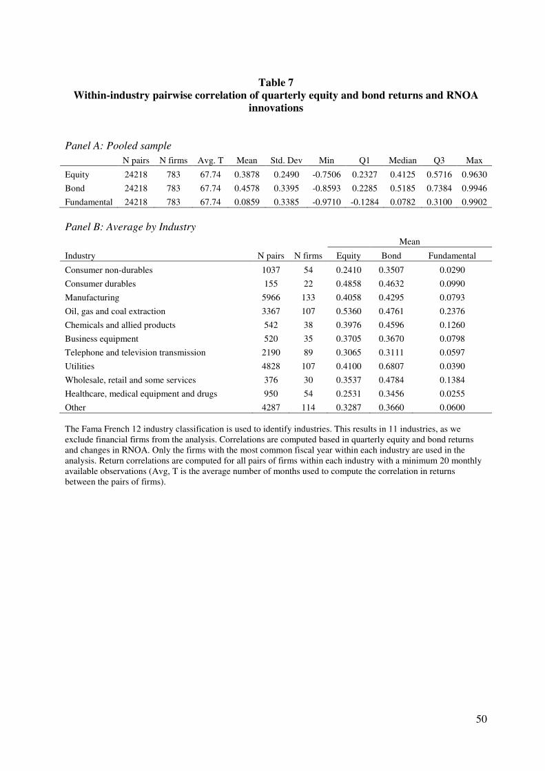
50

Table 7

Within-industry pairwise correlation of quarterly equity and bond returns and RNOA

innovations

Panel A: Pooled sample

N pairs N firms Avg. T Mean Std. Dev Min Q1 Median Q3 Max

Equity 24218 783 67.74 0.3878 0.2490 -0.7506 0.2327 0.4125 0.5716 0.9630

Bond 24218 783 67.74 0.4578 0.3395 -0.8593 0.2285 0.5185 0.7384 0.9946

Fundamental 24218 783 67.74 0.0859 0.3385 -0.9710 -0.1284 0.0782 0.3100 0.9902

Panel B: Average by Industry

Mean

Industry N pairs N firms Equity Bond Fundamental

Consumer non-durables 1037 54 0.2410 0.3507 0.0290

Consumer durables 155 22 0.4858 0.4632 0.0990

Manufacturing 5966 133 0.4058 0.4295 0.0793

Oil, gas and coal extraction 3367 107 0.5360 0.4761 0.2376

Chemicals and allied products 542 38 0.3976 0.4596 0.1260

Business equipment 520 35 0.3705 0.3670 0.0798

Telephone and television transmission 2190 89 0.3065 0.3111 0.0597

Utilities 4828 107 0.4100 0.6807 0.0390

Wholesale, retail and some services 376 30 0.3537 0.4784 0.1384

Healthcare, medical equipment and drugs 950 54 0.2531 0.3456 0.0255

Other 4287 114 0.3287 0.3660 0.0600

The Fama French 12 industry classification is used to identify industries. This results in 11 industries, as we

exclude financial firms from the analysis. Correlations are computed based in quarterly equity and bond returns

and changes in RNOA. Only the firms with the most common fiscal year within each industry are used in the

analysis. Return correlations are computed for all pairs of firms within each industry with a minimum 20 monthly

available observations (Avg, T is the average number of months used to compute the correlation in returns

between the pairs of firms).

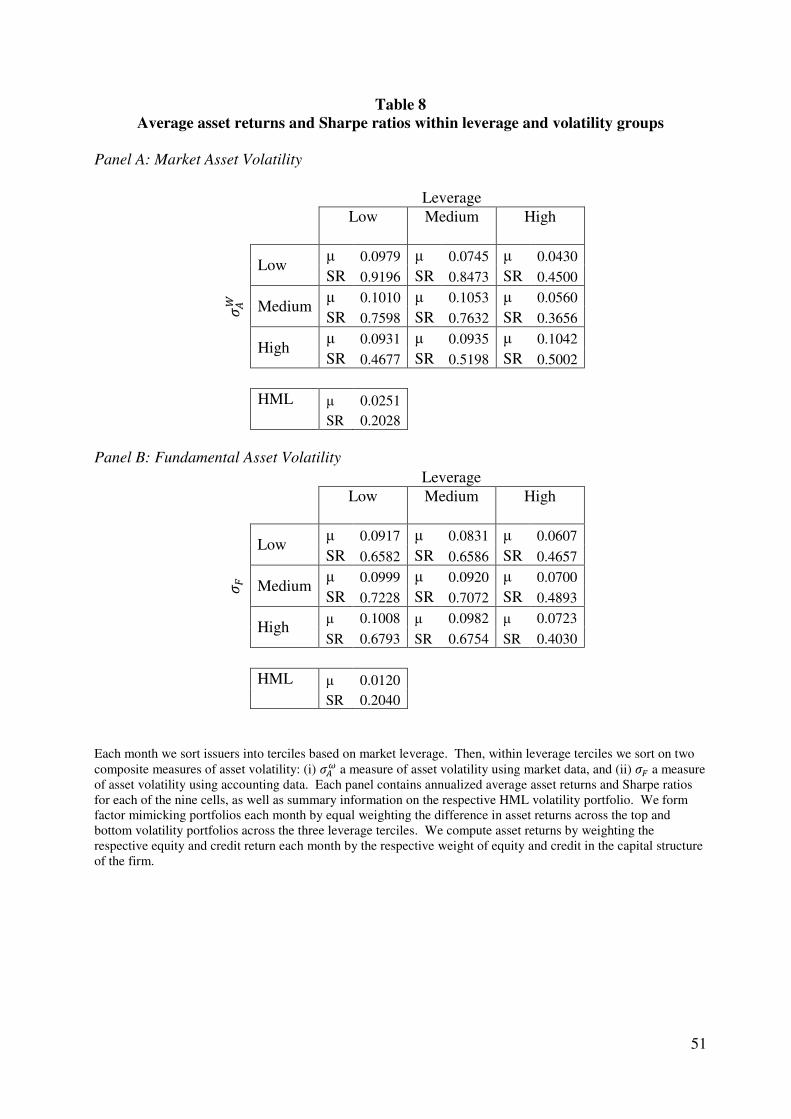
51

Table 8

Average asset returns and Sharpe ratios within leverage and volatility groups

Panel A: Market Asset Volatility

Leverage

Low

Medium

High

� ��

Low µ 0.0979 µ 0.0745 µ 0.0430

SR 0.9196 SR 0.8473 SR 0.4500

Medium µ 0.1010 µ 0.1053 µ 0.0560

SR 0.7598 SR 0.7632 SR 0.3656

High µ 0.0931 µ 0.0935 µ 0.1042

SR 0.4677 SR 0.5198 SR 0.5002

HML µ 0.0251

SR 0.2028

Panel B: Fundamental Asset Volatility

Leverage

Low

Medium

High

� =

Low µ 0.0917 µ 0.0831 µ 0.0607

SR 0.6582 SR 0.6586 SR 0.4657

Medium µ 0.0999 µ 0.0920 µ 0.0700

SR 0.7228 SR 0.7072 SR 0.4893

High µ 0.1008 µ 0.0982 µ 0.0723

SR 0.6793 SR 0.6754 SR 0.4030

HML µ 0.0120

SR 0.2040

Each month we sort issuers into terciles based on market leverage. Then, within leverage terciles we sort on two

composite measures of asset volatility: (i) �� a measure of asset volatility using market data, and (ii) �= a measure

of asset volatility using accounting data. Each panel contains annualized average asset returns and Sharpe ratios

for each of the nine cells, as well as summary information on the respective HML volatility portfolio. We form

factor mimicking portfolios each month by equal weighting the difference in asset returns across the top and

bottom volatility portfolios across the three leverage terciles. We compute asset returns by weighting the

respective equity and credit return each month by the respective weight of equity and credit in the capital structure

of the firm.

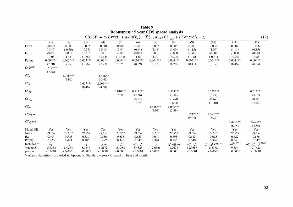
52

Table 9

Robustness : 5 year CDS spread analysis 0],53# = V)4QRS># + V LM(4#) + ∑ VB� WBG) 0,hr,O + X0YM>RYL# + F# (12)

(1) (2) (3) (4) (5) (6) (7) (8) (9) (10) (11) (12)

Exret -0.003 -0.003 -0.002 -0.001 0.003 0.003 0.007 0.006 0.007 0.006 0.007 0.006

(-0.40) (-0.56) (-0.36) (-0.11) (0.44) (0.44) (1.14) (1.00) (1.15) (1.00) (1.11) (0.85)

ln(E) -0.000 0.001 0.001* 0.001 -0.001 -0.001 0.001 -0.000 0.001 -0.000 -0.000 -0.001

(-0.08) (1.41) (1.76) (1.64) (-1.43) (-1.64) (1.10) (-0.21) (1.08) (-0.21) (-0.20) (-0.88)

Rating 0.004*** 0.003*** 0.003*** 0.003*** 0.004*** 0.004*** 0.004*** 0.004*** 0.004*** 0.004*** 0.004*** 0.004***

(7.50) (7.29) (7.56) (7.73) (9.25) (8.89) (8.13) (8.20) (8.11) (8.19) (8.46) (8.34) 0,hx{�C� 1.217***

(7.68) 0,hx 1.728*** -1.416**

(7.90) (-2.43) 0,hw 1.667*** 2.906***

(8.46) (4.68) 0,hcz 0.910*** 0.917*** 0.563*** 0.557*** 0.612***

(8.24) (7.56) (3.34) (3.27) (3.07) 0,hcwz -0.129 -0.470 -0.463 -0.180

(-0.48) (-1.44) (-1.40) (-0.52) 0,hs 1.888*** 1.066***

(9.04) (5.39) 0,tu1t1 1.891*** 1.072***

(9.04) (5.29) 0,hsvcwbx 1.426*** 0.649**

(6.15) (2.55)

Month FE Yes Yes Yes Yes Yes Yes Yes Yes Yes Yes Yes Yes

Nobs 29,557 29,557 29,557 29,557 29,557 29,557 29,557 29,557 29,557 29,557 29,557 29,557

R2 0.404 0.505 0.530 0.536 0.653 0.653 0.641 0.695 0.643 0.695 0.622 0.676

R2(U) 0.423 0.423 0.486 0.487 0.345 0.345 0.344 0.346 0.340 0.346 0.340 0.347

Included � �� �� �� �� , �� �� ��, ��� �= ��, ���, �= ��, ��� ��, ���, 29525 �=����� ��, ���, �=�����

Vuong Z -5.6358 8.0274 5.9347 6.2172 5.4388 5.4525 12.6666 8.2671 12.3688 8.3368 9.354 7.7629

p-value <0.0001 <0.0001 <0.0001 <0.0001 <0.0001 <0.0001 <0.0001 <0.0001 <0.0001 <0.0001 <0.0001 <0.0001

Variable definitions provided in Appendix. Standard errors clustered by firm and month.