


Languages
Pages
Legal

Assessing Inter-generational Mobility:
A Functional Data Regression Approach
Pierre Chausse∗1, Tao Chen†1,2 and Kenneth A. Couch‡3
1Department of Economics, University of Waterloo, Ontario, Canada
2Big Data Research Center, Jianghan University, Hubei, China
3Department of Economics, University of Connecticut, Connecticut, USA
Abstract
This paper extends functional data analysis to circumstances where researchers encounter time-
varying models with functional dependent variables and multiple functional covariates and have to
handle missing values in the underlying panel data under sign restrictions. Results from a sim-
ulation study suggest that our method can work very well even in small (both N and T ) sized
samples when other traditional approaches fail. Our algorithm is applied to the estimation of the
intergenerational elasticity of earnings using data from the Panel Study of Income Dynamics. Es-
timates based on the functional data approach indicate that the modern literature has somewhat
over-estimated the strength of the average relationship between earnings of fathers and sons and
that earnings for fathers earlier in the sons’ lives have a greater impact on their future earnings.
1

1 Introduction
In many applied research contexts, panel data that contain numerical values of labor market and other
economic outcomes that can naturally take the value of zero are used. Often, it is desirable to express
these outcomes, particularly earnings, in logs as they are highly skewed distributions that appear log
normal. This creates a practical issue of how to address the censoring that occurs at zero.
Using studies in the empirical literature measuring intergenerational mobility in earnings as an
example, well known studies have either dropped all data for pairs of fathers and sons when one or more
observations of zero are present in the panel observations (Cf. Solon (1992)) or similarly have required
the fathers and sons to be fully employed in each panel observation to enter the estimation sample (Cf.
Zimmerman (1992)). Procedures of these types raise obvious concerns about selection bias if recovering
estimates of population parameters is the goal of the analysis. Here, we propose the use of functional
data analysis (FDA) as a method of smoothing data observations in panel settings with censoring of
this type.1
The contributions of this paper are threefold: (1) we extend prior functional regression studies that
had considered the case of a single functional covariate to the multi-covariate context (Cf. Ramsay and
Dalzell (1991, Chapter 16)). We find that compared to traditional multiple regression, a new identi-
fication condition is necessary for functional multi-covariate regressions. (2) We explore properties of
multi-covariate functional estimation in the presence of the aforementioned censoring for both depen-
dent and independent variables in Monte Carlo simulations. (3) We apply our algorithm to estimate the
intergenerational correlation in earnings using data from the Panel Study of Income Dynamics (PSID)
as an empirical study.
FDA was first developed in the seminal work of Ramsay and Dalzell (1991) and most of its applica-
tions have been in Biomedical Science and Biomechanics since then. Recently, researchers have started
applying FDA to other areas like Marketing (Wang et al. (2008) and Sood et al. (2009)), Operational
Research (Laukaitis (2008)), and Sports (Chen and Fan (forthcoming)), just to name a few. The only
1A recent study by Chen and Couch (2015) proposed a method-of-moment-type data driven method to address similar
issue; however, the validity of that method is unknown when the parameters of interest are time varying.
2

application in Economics we are aware of is Ramsay and Ramsey (2002).
Conceptually, the advantages of FDA are the following: (1) unlike traditional linear regressions,
functional regression allows both the dependent and independent variables to be functions (usually in
terms of time). Therefore, in this more general setting, the parameters of interest are not constants
anymore, but functions, which accommodate time-varying properties naturally. Using our empirical
study as an example, we will be able to estimate the impact of a father’s income when the father was
at age t on the son’s income when the son is at age τ for all the possible pairs of (t, τ), while all the
previous studies have assumed this impact is the same across different combinations of t’s and τ ’s. (2)
Given the fact that we can only collect data discretely even when the underlying data generating process
(DGP) is continuous, there is a potential risk of invalid statistical inference based on estimates from
discrete models (Cf. Merton (1980) and Aıt-Sahalia (2002)). FDA does not suffer from this issue.
Next we develop the notation for a general functional regression model that allows for multiple inde-
pendent regressors extending the work of Ramsay and Silverman (2005). In Section 2, basic inferential
formulas for the parameters of the model are provided. Then, Section 3 provides a numerical simulation
of key features of the model. Section 4 goes further to reconsider a well known empirical example,
the relationship of the labor earnings of sons to their fathers through the estimated intergenerational
elasticity. Section 5 contains the conclusion.
2 Functional Data Regression with functional dependent vari-
able and multi-covariate functional independent variables
Statistical analysis involving functional data usually starts with estimating the underlying functional
data Yi(t) ∈ Y, where Y is the set of continuous functions in t, from a panel Yit of observations, with
i = 1, ..., N and t = 1, ..., T . We view the Yi(t) observations as independent random functions.
Following Ramsay and Silverman (2005, Equation 3.1), we assume that Yit = Yi(t) + εit, where the
εit’s are mutually independent zero mean and finite variance random variables. It is well known that
any function can be approximated arbitrarily well by a linear combination of a sufficiently large number
3
of basis functions.2 Therefore, we let Yi(t) be expressed as
Yi(t) ≈k∑j=1
cijφj(t) = c′iφ(t), (1)
where φj(t) are the known basis functions and cij are the corresponding Fourier coefficients which will
be obtained by minimizing the following penalized least-squares-type objective function:
PSSRi(ci, λ, k) =T∑t=1
(Yit − c′iφ(t))2
+ λ
[∫ (d2Yi(t)
dt2
)2
dt
]
=T∑t=1
(Yit − c′iφ(t))2
+ λc′i
[∫ (d2φ(t)
dt2
)(d2φ(t)
dt2
)′dt
]ci. (2)
It is obvious that the PSSR objective function reflects one of the most fundamental principals in Statistics
by balancing the bias and variance of the estimates.
The estimation of ci’s is done separately for each i given the smoothing parameter λ and the number
of basis functions k, but the choice of λ and k are determined jointly by all i’s because we assume the
Yi(t)’s share the same smoothness. We choose the λ and k that minimize the following leave-one-out
cross-validation (LCV).
LCV(λ, k) =N∑i=1
LCVi(λ, k) =N∑i=1
[T∑t=1
(Yit − Y −tit )2
], (3)
where Y −tit = (c−ti )′φ(t) and c−ti is the estimate obtained by removing the observation at time t. Ramsay
and Silverman (2005) propose a generalized cross-validation method to reduce computation time but
its validity depends on the assumption that the residuals are homogeneous which might not be realistic
for the income paths that we will be estimating. Therefore we choose not to use it. Note that the LCV
function is smooth in λ for a given k. Hence, we can easily obtain the optimal λ for each k using a fast
and reliable univariate method such as the Brent algorithm, and then search over the k’s.
2For a detailed discussion of basis function, we refer the reader to Ramsay and Silverman (2005, Sections 3.3-6).
4

2.1 Positive Functional Data
When recovering the underlying functional data, researchers sometimes want to impose sign restrictions.
For example, in the intergenerational mobility study, we are interested in the elasticity of childrens’
earnings with respect to their parents’. Due to the log normalities of earnings, we want to express
earnings in logarithms. If all observations were positive, we could estimate the functional data from
log(Yit). However, this approach is not feasible when some observations are equal to zero. We can
think of the presence of a zero as being the result of a market shock which may depend on individual
characteristics, but is not representative of true income potential, which should be strictly positive.
One way to fit a strictly positive functional data to the sample is to assume the following represen-
tation for Yi(t):
Yi(t) ≈ ec′iφ(t). (4)
The choice of the exponential function is related to the need to express Yi(t) in logarithms. Once the
ci vector is estimated, we can define the logarithm of Yi(t) as log Yi(t) = c′iφ(t). The estimation with
this transformation is, however, more difficult because the solution does not have a closed form implied
by Equation (2) directly. Instead, we need to minimize the following penalized non-linear least squares
function:
NLPSSRi(λ(k), k) =T∑t=1
(Yit − ec
′iφ(t))2
+ λc′i
∫ (d2φ(t)
dt2
)(d2φ(t)
dt2
)′dtci. (5)
. The parameters λ and k can also be selected by minimizing the LCV of Equation (3), with
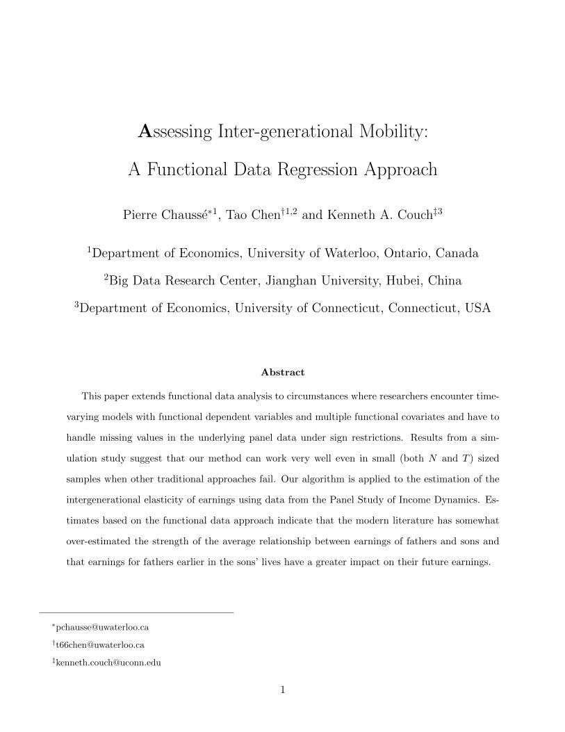
Y −tit = e(c−ti )′φ(t) 3. Figure 1 illustrates the fitted functional data for one observation with three zeros out
of five time units, for two values of k and λ. We can see that the shape of the fit varies with the choice
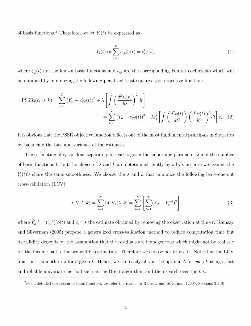
of k and λ. Figure 2 shows the same data with the estimated curve based on the optimal λ∗ = 0.7639
and k∗ = 7.
When T is small, it becomes difficult to compute the LCV. First, we cannot fit a strictly positive
3To compute the LCV, it is required to solve NT penalized non-linear least squares problems. However, the compu-
tation is done efficiently in the funcreg package for R, using a Newton method with line search in which the derivatives
are computed analitically. The entired algorithm is written in Fortran 90.
5

functional data on observations with only zero elements, which implies that it is impossible to compute
the LCV when only one element is non-zero. It does not mean that we have to omit observations with
only one non-zero element but we cannot base our choice of the smoothing parameters λ and k on
those observations. Furthermore, when the number of non-zero elements is equal to two and T is small
(T = 5 in the application below), the non-linear algorithm used to compute the c−ti ’s sometimes fails to
converge, which also prevents us from computing the LCV. 4 Figure 3 shows what happens when the
algorithm fails to converge. The smoothing parameter λ becomes inoperative and the function overfits
the data points.5
What we propose to avoid complications regarding the computation of the LCV when T is small
and zeros are present is to base the choice of λ and k on observations with no zero element. We assume
that the level of smoothness does not depend on whether zeros are observed or not. Once the optimal
smoothing parameters are obtained we then fit a functional data to each i.
2.2 Multiple Functional Regression
Because previous research using functional regression only considered a single covariate but many com-
mon applications including the one considered here are multi-covariate, we provide the necessary deriva-
tion for the multivariate case. We also discuss the identification for the multi-covariate case. For the
complete derivation, see Appendix A. We write the general model as:
yi(t) = β0(t) +
q∑j=1
∫Ω
βj(s, t)xij(s)ds+ εi(t). (6)
4The main problem comes from the fact that R is by construction positive semi-definite. It therefore becomes possible
that the NLPSSR reaches a flat region in which c′iRci is nearly zero.
5It is important to note that c′iRci can be numerically negative for some ci even if R is positive semi-definite, which
complicates the minimization of the NLPSSR. To avoid such numerical problem, c′iRci is computed using its eigenvalues
representation in which all eigenvalues less than the square root of the machine-epsilon in absolute value are set to 0.
6
1.0 1.2 1.4 1.6 1.8 2.0
0.0
0.4
0.8
t
Y(t
)
λ = 1e−05 , k = 7λ = 1e−05 , k = 9λ = 0.01 , k = 7λ = 0.01 , k = 9
Figure 1: Positive functional data fit for an observation with three zeros
1.0 1.2 1.4 1.6 1.8 2.0
0.0
0.4
0.8
t
Y(t
)
Figure 2: Positive functional data fit with three zero and optimal λ∗ = 0.7639 and k∗ = 7.
7

1.0 1.2 1.4 1.6 1.8 2.0
0.00
0.02
0.04
t
Y(t
)
Figure 3: Convergence problem with only one non-zero element
yi(t) refers to a functional outcome of unit i indexed by time t. β0(t) is the intercept function. βj(s, t)’s
are bi-variate slope functions indexed by time t and s jointly. The variable xij(s), j = 1, ..., q, is a set
of independent variables that influence individual i outcomes. s indexes the timing of xij(s). εi(t) is
assumed to be an i.i.d. error term. q indexes the regressors.
Here we assume that the integrals are evaluated over a common interval Ω. So, for notational
simplicity, we suppress the reference to Ω throughout the paper. In some cases, it may be more ap-
propriate to allow regressors to affect yi(t) over different time intervals. Nonetheless, that extension is
straightforward and would primarily complicate the exposition.
Before presenting the details about the estimation method, we want to briefly discuss the identi-
fication issue. We can see in the following that βj(s, t) not being additively separable is a necessary
condition for identification. This identification condition is new to the literature. Suppose q = 1 and
8

β1(s, t) = α(s) + θ(t). Then,
yi(t) = β0(t) +
∫α(s)xi(s)ds+ θ(t)
∫xi(s)ds+ εi(t)
= β0(t) + const. + θ(t)
∫xi(s)ds+ εi(t)
For fixed T and N going to infinity θ(t) is not identified. The intuition behind this is the same as the
“incidental parameters problem” in panel data analysis (see Lancaster (2000) for a good overview of
this problem in econometrics). This is not surprising, as functional data is after all a continuous version
of the panel data we observe.
Following the results from the previous section, we assume that each functional data vector can be
correctly approximated by a linear combination of basis functions. So we can write:
yi(t) ≈ C ′yiφy(t),
and
xij(s) ≈ C ′xijφxj(s).
For the functional coefficients, we approximate the functional β0(t) as:
β0(t) ≈k0∑l=1
C0lφ0l(t) = C ′0φ0(t)
and the bivariate functional coefficient βj(s, t) as:
βj(s, t) ≈ksj∑l=1
ktj∑r=1
Cjlrφsjl(s)φtjr(t) = φ′sj(s)Cjφtj(t)
The number of basis in β0(t) and βj(s, t) are smoothing parameters that will need to be selected.
Equation (6) can be written in a more compact way as:
y(t) = W (t)γ + ε(t). (7)
9
where γ is a vector containing all elements of C0 and Cj, and the estimator γ is
γ =
[∫W ′(t)W (t)dt+R(λ)
]−1 [∫W ′(t)y(t)dt
], (8)
where the definitions of W and R(λ) could be found in the Appendix. We assume that the penalty is
based on the second derivative of the functional parameters, but we could easily modify the estimator
for a different type of penalty. For each derivative, we have a smoothing parameter that puts a weight
on it. For the intercept β0(t), we only have one smoothing parameter, λ0, that penalizes its second
derivative. However, for each βj(s, t), we want to penalize its second derivative with respect to t with
λtj and its second derivative with respect to s with λts. We therefore have two smoothing parameters
per functional slope, λtj, λsj. As a result, we have a total of 2q + 1 smoothing parameters to select.
All the smoothing parameters can be selected based on the following LCV:
LCVreg(λ) =N∑i=1
∫[yi(t)− y−ii (t)]2dt, (9)
where y−ii is the estimated value of yi(t) with the ith observation omitted and λ = (λ0, λs1, λt1, ..., λsq, λtq)′.
The minimization is done by applying the Nelder-Mead simplex method to LCVreg(λ), which only re-
quires function evaluations.
What is not explicit in Equation (9) is that the LCVreg also depends on the number of bases k0, ksj
and ktj, which gives us a total of 2q + 1 integers to choose. However, we have to consider that for a
large number of bases, the system of linear equations that we need to solve in Equation (8) can become
badly conditioned or simply singular. An easier way to proceed is to set the number of bases k0, ksj’s
and kjj’s to a large number and to use a ridge-regression type of regularization. That reduces the choice
of the (2q + 1) parameters kxx’s to the choice of a single continuous regularization parameter α. The
estimator of γ becomes
γ =
[∫W ′(t)W (t)dt+R(λ) + αI
]−1 [∫W ′(t)y(t)dt
], (10)
10

2e−06 4e−06 6e−06 8e−06 1e−05
67.5
68.5
69.5
α
LCV
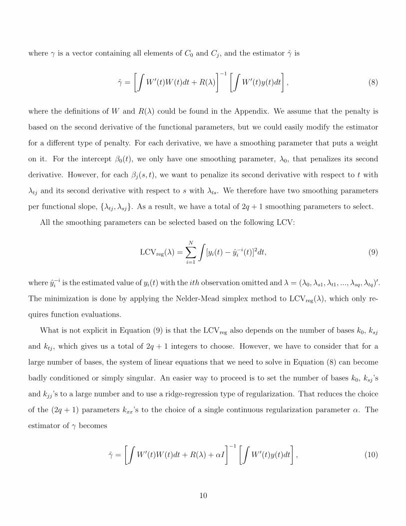
Figure 4: LCVreg(α, λ) given λi = 10−5 ∀i
where I is the identity matrix. The cross-validation defined in Equation (9) becomes a function of λ and
α. As an estimation strategy, we propose to obtain α and λ separately because LCVreg(α, λ) is a smooth
function of α for a given λ. Using one sample from our simulation exercise below, Figure 4 shows what
the LCVreg(α, λ) function looks like for a fixed vector λ. It is therefore easy to obtain the optimal α
using an univariate minimization algorithm. The procedure is done in four steps: (i) set λ to an initial
value, λ0, and compute α0 which minimizes LCVreg(α, λ0), (ii) compute λ1 by minimizing LCVreg(α0, λ),
(iii) recompute a final α, α, for λ = λ1, and (iv) compute the final λ by minimizing LCVreg(α, λ)6.
3 Monte Carlo Experiment
In this section, we analyze the properties of the multi-covariate functional regression in terms of its ability
to recover βj’s. For the latter, we compare the properties of βj obtained from the functional regression
6The purpose of the algorithm is to reduce the computational complexity of minimizing LCVreg. This approach is
closely related to the Coordinate Descent algorithm (Cf. Wright (2015)). The choice of stopping after two iterations is to
speed up the Monte Carlo experiment. Also, we did not find much improvement by increasing the number of iterations.
11
approach versus the ordinary least square (OLS) estimator. In particular, we want to use a DGP
that produces zeros and see how the functional regression approach that incorporates all observations
compares to using OLS, which by implication drops observations with zeros.
The DGP is defined as:
y∗i (t) = β0(t) +
∫ 2
1
β1(s, t)xi1(s)ds+
∫ 2
1
β2(s, t)x∗i2(s)ds+ εi(t). (11)
We let β1(s, t) = s× t and β2(s, t) = exp(sin(s + t)). Also, xi1(s) = Ui × s, where Ui’s are drawn from
an independent uniform random variable from 0 to 1. x∗i2(s) = Vi + (s − 1.5)2, where Vi’s are drawn
from an independent uniform random variable from c1 to c2. εi(t)’s are independent standard normal
random variables. We adjust c1 and c2 to control the censoring level of x2 := x∗21x∗2 > 0 and β0 for
the censoring level of y := y∗1y∗ > 0.
We calibrate the distribution of Vi to have a level of censoring of x∗2 between [αlx, αux]. Since (s−1.5)2 ∈
[0, 0.25], c1 and c2 must be such that F (0) = αux and F (−0.25) = αlx. We therefore have:
c1 = − 0.25αuxαux − αlx
and
c2 =0.25(1− αux)
αux − αlx.
Therefore, for censoring from 10% to 30%, we must have Vi ∼ U(−0.375, 0.875). We can rewrite the
process as
yi(t)∗ = β0 +
7
3Uit+ ViI1(t) + I2(t) + εi(t),
where
I1(t) =
∫ 2
1
exp(sin(s+ t))ds
and
I2(t) =
∫ 2
1
exp(sin(s+ t))(s− 1.5)2ds.
12
1.0 1.2 1.4 1.6 1.8 2.0
−2
02
46
t
y(t)
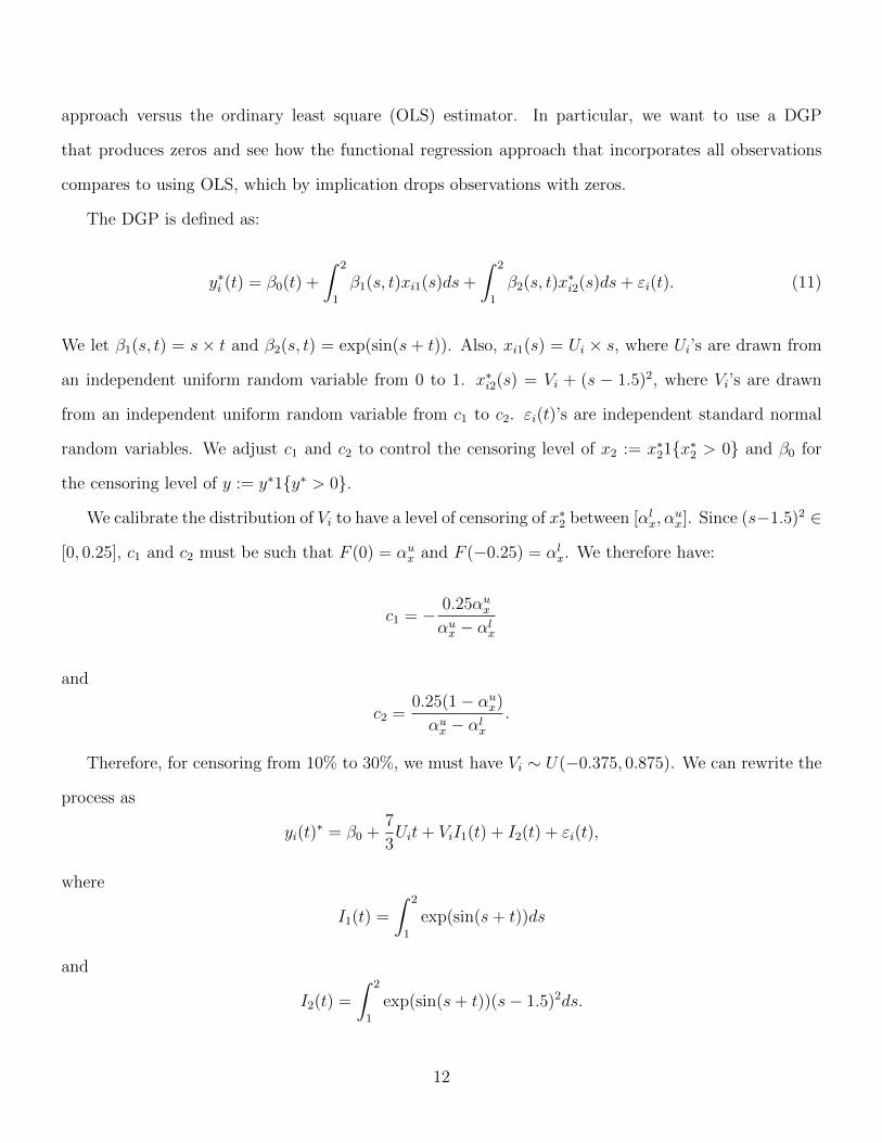
Figure 5: Fitted functional data y(t) withoutrestricting the curves to be positive
1.0 1.2 1.4 1.6 1.8 2.0
01
23
45
6
t
y(t)
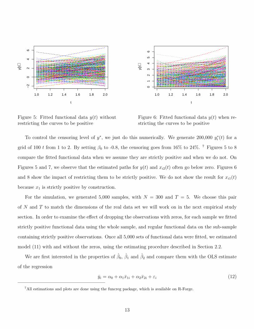
Figure 6: Fitted functional data y(t) when re-stricting the curves to be positive
To control the censoring level of y∗, we just do this numerically. We generate 200,000 y∗i (t) for a
grid of 100 t from 1 to 2. By setting β0 to -0.8, the censoring goes from 16% to 24%. 7 Figures 5 to 8
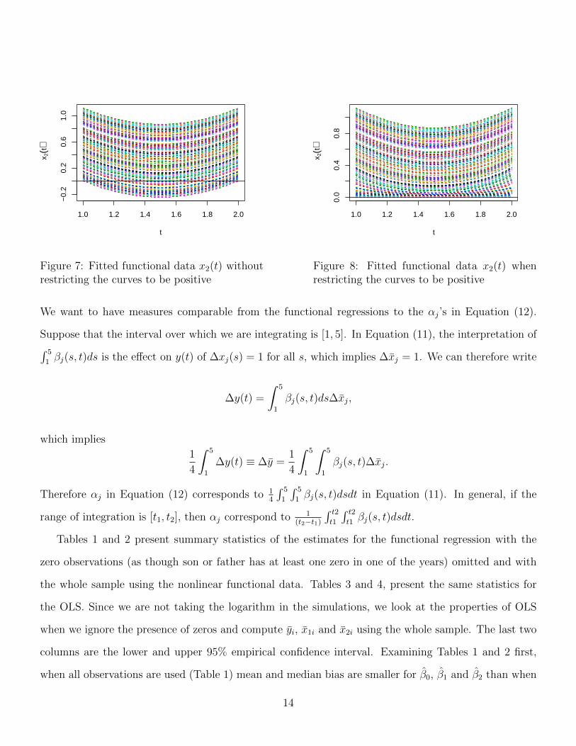
compare the fitted functional data when we assume they are strictly positive and when we do not. On
Figures 5 and 7, we observe that the estimated paths for y(t) and xi2(t) often go below zero. Figures 6
and 8 show the impact of restricting them to be strictly positive. We do not show the result for xi1(t)
because x1 is strictly positive by construction.
For the simulation, we generated 5,000 samples, with N = 300 and T = 5. We choose this pair
of N and T to match the dimensions of the real data set we will work on in the next empirical study
section. In order to examine the effect of dropping the observations with zeros, for each sample we fitted
strictly positive functional data using the whole sample, and regular functional data on the sub-sample
containing strictly positive observations. Once all 5,000 sets of functional data were fitted, we estimated
model (11) with and without the zeros, using the estimating procedure described in Section 2.2.
We are first interested in the properties of β0, β1 and β2 and compare them with the OLS estimate
of the regression
yi = α0 + α1x1i + α2x2i + εi (12)
7All estimations and plots are done using the funcreg package, which is available on R-Forge.
13
1.0 1.2 1.4 1.6 1.8 2.0
−0.
20.
20.
61.
0
t
x 2(t)
Figure 7: Fitted functional data x2(t) withoutrestricting the curves to be positive
1.0 1.2 1.4 1.6 1.8 2.0
0.0
0.4
0.8
t
x 2(t)
Figure 8: Fitted functional data x2(t) whenrestricting the curves to be positive
We want to have measures comparable from the functional regressions to the αj’s in Equation (12).
Suppose that the interval over which we are integrating is [1, 5]. In Equation (11), the interpretation of∫ 5
1βj(s, t)ds is the effect on y(t) of ∆xj(s) = 1 for all s, which implies ∆xj = 1. We can therefore write
∆y(t) =
∫ 5
1
βj(s, t)ds∆xj,
which implies
1
4
∫ 5
1
∆y(t) ≡ ∆y =1
4
∫ 5
1
∫ 5
1
βj(s, t)∆xj.
Therefore αj in Equation (12) corresponds to 14
∫ 5
1
∫ 5
1βj(s, t)dsdt in Equation (11). In general, if the
range of integration is [t1, t2], then αj correspond to 1(t2−t1)
∫ t2t1
∫ t2t1βj(s, t)dsdt.
Tables 1 and 2 present summary statistics of the estimates for the functional regression with the
zero observations (as though son or father has at least one zero in one of the years) omitted and with
the whole sample using the nonlinear functional data. Tables 3 and 4, present the same statistics for
the OLS. Since we are not taking the logarithm in the simulations, we look at the properties of OLS
when we ignore the presence of zeros and compute yi, x1i and x2i using the whole sample. The last two
columns are the lower and upper 95% empirical confidence interval. Examining Tables 1 and 2 first,
when all observations are used (Table 1) mean and median bias are smaller for β0, β1 and β2 than when
14

they are dropped (Table 2). The root-mean-square error (RMSE) is also smaller and the estimates are
estimated more precisely when all data observations are included (Table 1). The estimates for the slope
parameters, β1 and β2 are within the 95% confidence intervals for the true parameters in Tables 1 and
2 although the estimates in Table 1 are preferred given their smaller bias. Note, β0 in Table 1 is outside
the 95% confidence interval reflecting the fact that estimation of the level might not be not credible due
to censoring without further structural assumptions, which we try avoid. Nevertheless, in most of the
cases, researchers are more interested in the slope functions.
Examining Tables 3 and 4, mean and median bias of the parameter estimates for β0, β1 and β2 are
also smaller when all observations are used with OLS (Table 3) as opposed to when observations of zero
are dropped (Table 4). RMSE and the standard deviations are also smaller when all observations are
included in the estimates. However, in Table 3, when all of the observations are included, the estimates of
both β0 and β1 lie outside a 95% confidence interval; this same result occurs in Table 4 when observations
of zero are dropped. Thus, OLS appears to perform less well in providing accurate estimates of the true
parameters in these simulations. The badly biased slope parameters are a particular concern.
True Mean-Bias Median Bias RMSE S-dev Lower-Conf upper-Conf
β0 -0.8000 0.3732 0.3746 0.3787 0.0641 -0.5524 -0.3011
β1 2.2500 0.0167 0.0455 0.1511 0.1502 1.9724 2.5610
β2 1.2210 -0.1045 -0.1048 0.1382 0.0905 0.9392 1.2939
Table 1: Estimated average coefficients by functional regression when all observations are included
True Mean-Bias Median Bias RMSE S-dev Lower-Conf upper-Conf
β0 -0.8000 0.4654 0.4670 0.5212 0.2346 -0.7944 0.1253
β1 2.2500 -0.2254 -0.2336 0.4992 0.4454 1.1515 2.8976
β2 1.2210 -0.1257 -0.1289 0.2022 0.1583 0.7850 1.4056
Table 2: Estimated average coefficients by functional regression when observations with zeros aredropped
For the Monte Carlo simulations, it is also possible to provide confidence surfaces for β1(s, t) and
β2(s, t) relative to the true parameters. A detailed discussion of the construction of the surfaces through
the concept of depth is provided in Appendix Section A.2. Figures 9 and 10 provide graphs of these
relationships using the two data sets from the Monte Carlo analysis either omitting zeros or not. Figure
15

True Mean-Bias Median Bias RMSE S-dev Lower-Conf upper-Conf
β0 -0.8000 0.3880 0.3885 0.3930 0.0626 -0.5346 -0.2893
β1 2.2500 -0.2450 -0.2446 0.2521 0.0594 1.8885 2.1214
β2 1.2210 -0.1373 -0.1375 0.1615 0.0851 0.9170 1.2505
Table 3: Estimated average coefficients by OLS when all observations are included
True Mean-Bias Median Bias RMSE S-dev Lower-Conf upper-Conf
β0 -0.8000 0.4630 0.4643 0.4887 0.1563 -0.6434 -0.0305
β1 2.2500 -0.2399 -0.2410 0.2641 0.1105 1.7935 2.2267
β2 1.2210 -0.1504 -0.1535 0.2156 0.1544 0.7679 1.3733
Table 4: Estimated average coefficients by OLS when observations with zeros are dropped
9 and 10 show the true value of β1(s, t) in the horizontal plane at 2.25. The surfaces above and below
the true plane provide a visual representation of the 95% confidence interval in this space. Figure 11
and 12 provide a similar plot for the true value of β2(s, t) shown in the horizontal plane at 1.22 while the
surfaces above and below it provide a visual representation of the confidence surfaces in this parameter
space. That the plane representing the true values of the parameters lie between the upper and lower
confidence surfaces provides further evidence the estimator performs well in instances of small T and N.
4 A Functional Regression Approach to Intergenerational Mo-
bility in Earnings of Sons and Fathers
Studies in what can reasonably be considered the early literature on intergenerational economic mobility
were based on cross-sectional data and short panels (Cf. Becker and Tomes (1986, Table 22)). Those
estimates often focused on estimation of the intergenerational correlation in earnings between sons and
fathers and ranged from about 0.2 to 0.4. The conceptual problem with reliance on cross-sectional data
to estimate a relationship between the permanent or long-run economic status of two generations is
that the available data for fathers and sons only represents a single point in time and the observation is
subject to measurement error. Thus, there is a difference in the observation of earnings at a point in time
and measures which gauge status over time that might be considered more typical of life experiences
16

β1(s, t)
1.01.2
1.41.6
1.82.0
1.01.2
1.41.6
1.82.0
−20
0
20
40
st
z
−20
0
20
40
60
Figure 9: Simulated results with zeros omitted
β1(s, t)
1.01.2
1.41.6
1.82.0
1.01.2
1.41.6
1.82.0
−5
0
5
10
15
st
z
−5
0
5
10
15
Figure 10: Simulated results with all observa-tions
β2(s, t)
1.01.2
1.41.6
1.82.0
1.01.2
1.41.6
1.82.0
−20
−10
0
10
20
st
z
−30
−20
−10
0
10
20
30
Figure 11: Simulated results with all with zerosomitted
β2(s, t)
1.01.2
1.41.6
1.82.0
1.01.2
1.41.6
1.82.0
−2
0
2
4
6
st
z
−4
−2
0
2
4
6
Figure 12: Simulated results with all observa-tions
17

than a static snapshot drawn from a single observation.
This insight led to the work of Solon (1992) and Zimmerman (1992) who modeled the difference
between permanent latent variables and observed quantities as falling into a classic errors-in-variables
model.8 The impact of the bias is shown in this model to reduce estimated intergenerational relationships
between earnings of two generations. If errors in this model are independent and identical, then averaging
observations over time yields a less noisy measure of permanent earnings. As the true parameter relating
son’s and father’s earnings is biased by a signal to noise ratio, averaging observations reduces the noise
relative to signal and should increase estimated elasticities and correlations in earnings. In both Solon
and Zimmerman’s work, it can be shown that using their samples, as earnings are averaged across
successive years for fathers the intergenerational correlation in earnings rises towards the upper end of
the range observed by Becker and Tomes (1986) in the prior literature.
In selecting the data for their studies (Solon (1992) and Zimmerman (1992)) pairs of fathers and sons
with values of earnings below a certain threshold for any of the time periods used in the calculations were
omitted or similarly, sample members were required to be fully employed. In part, these adjustments to
the data address the problem of the natural logarithm of zero being undefined.
Conceptually, when longer periods of data are used and individuals are attrited if their income goes
below a threshold, the question arises of whether the resulting estimates that arise are driven by to the
increasingly restrictive sample criteria as additional informational demands are imposed on the selection
rule for an individual to enter the estimates. Couch and Lillard (1998) use the same sources of panel
data as the two prior studies which argued the larger correlations in earnings were due to omitted
variable bias, and demonstrate that when sample observations are not omitted due to low earnings or
intermittent employment, that estimates of the intergenerational elasticity and correlation in earnings
do not rise as averages of earnings are carried out over additional years of observations. The work of
Freeman (1981) and others contain similar findings in that when earnings observations are not screened,
measures of intergenerational relationships in earnings are indicative of more mobility. While the work
8Slightly earlier work which used multiple years of observations from panel data to measure intergenerational correla-
tions in economic status and drew similar qualitative conclusions can be found in Altonji and Dunn (1991)
18

of Couch and Lillard (1998) as well as the results from other studies that have not screened out low
earnings observations points towards the potential usefulness of different approaches to the widely used
estimation procedure for gauging intergenerational correlations and elasticities in earnings, the solution
offered there, to add $1 to each observation and proceed with the method proposed in the work of Solon
(1992) and Zimmerman (1992), it is not well grounded theoretically.
One possible approach to resolving this issue is demonstrated in the work of Haider and Solon
(2006). Pairwise estimates of Tobits can be estimated assuming a bivariate normal density.9 The
resulting estimates can be used in a Minimum Distance framework to infer cross-period correlations
in residual earnings. A concern with this approach is potential bias imposed by the structure of the
assumptions made to support the estimation procedure.
Here, we apply the functional regression approach to estimate the intergenerational elasticity of
earnings using the PSID. The data includes 309 fathers and sons over 5 periods (1967 to 1971 for the
fathers and 1983 to 1987 for the sons). The proportion of the sample that would be omitted if all father
and son pairs that contain at least one zero were dropped is 18%. The discrete model is
ys = β0 + β1yf + β2Af + β3A2f + β4As + β5A
2s + u, (13)
where ys and yf are the log average of sons and fathers earnings. To compare with previous studies,
we show in Table 5 the estimates of the intergenerational elasticity in earnings using the approaches
of Solon (1992) and Couch and Lillard (1998). In the first case, observations where either a father or
son had an observation of zero are omitted and in the second, zeros are replaced by ones. For each
method, we estimate the model with and without the age-squared variables because their coefficients
are not statistically significant at the 5% level. We can see that including all observations and replacing
zeros with ones substantially reduces the estimated elasticity, the parameter estimate associated with
yf which implies higher intergenerational mobility.
For the functional regression approach, we estimated the intergenerational elasticity using the fol-
9This method is also used in a different context in Couch et al. (1999).
19
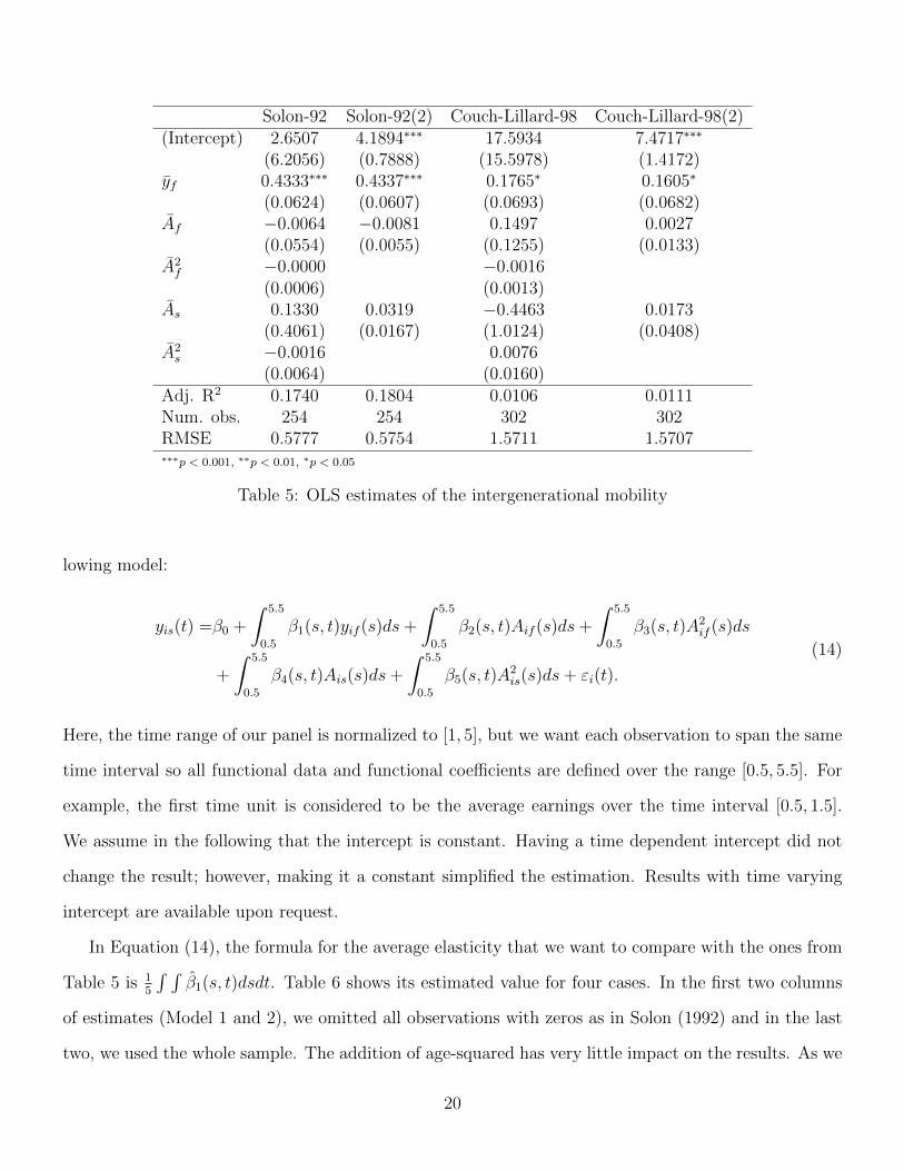
Solon-92 Solon-92(2) Couch-Lillard-98 Couch-Lillard-98(2)(Intercept) 2.6507 4.1894∗∗∗ 17.5934 7.4717∗∗∗
(6.2056) (0.7888) (15.5978) (1.4172)yf 0.4333∗∗∗ 0.4337∗∗∗ 0.1765∗ 0.1605∗
(0.0624) (0.0607) (0.0693) (0.0682)Af −0.0064 −0.0081 0.1497 0.0027
(0.0554) (0.0055) (0.1255) (0.0133)A2f −0.0000 −0.0016
(0.0006) (0.0013)As 0.1330 0.0319 −0.4463 0.0173
(0.4061) (0.0167) (1.0124) (0.0408)A2s −0.0016 0.0076
(0.0064) (0.0160)Adj. R2 0.1740 0.1804 0.0106 0.0111Num. obs. 254 254 302 302RMSE 0.5777 0.5754 1.5711 1.5707∗∗∗p < 0.001, ∗∗p < 0.01, ∗p < 0.05
Table 5: OLS estimates of the intergenerational mobility
lowing model:
yis(t) =β0 +
∫ 5.5
0.5
β1(s, t)yif (s)ds+
∫ 5.5
0.5
β2(s, t)Aif (s)ds+
∫ 5.5
0.5
β3(s, t)A2if (s)ds
+
∫ 5.5
0.5
β4(s, t)Ais(s)ds+
∫ 5.5
0.5
β5(s, t)A2is(s)ds+ εi(t).
(14)
Here, the time range of our panel is normalized to [1, 5], but we want each observation to span the same
time interval so all functional data and functional coefficients are defined over the range [0.5, 5.5]. For
example, the first time unit is considered to be the average earnings over the time interval [0.5, 1.5].
We assume in the following that the intercept is constant. Having a time dependent intercept did not
change the result; however, making it a constant simplified the estimation. Results with time varying
intercept are available upon request.
In Equation (14), the formula for the average elasticity that we want to compare with the ones from
Table 5 is 15
∫ ∫β1(s, t)dsdt. Table 6 shows its estimated value for four cases. In the first two columns
of estimates (Model 1 and 2), we omitted all observations with zeros as in Solon (1992) and in the last
two, we used the whole sample. The addition of age-squared has very little impact on the results. As we
20

would expect, removing the zeros increases the standard errors of the parameter estimates. As far as the
estimate of the intergenerational elasticity of earnings is concerned, we get very similar results to those
based on OLS when we omit the zeros. Including the zeros, however, in conjunction with functional
regression reduces the estimate and its standard error, which is consistent with our simulation results.
The estimated elasticities in Models 3 and 4 lie between those obtained ignoring zeros or setting them
to one in Table 5. By setting the zeros to one, Couch and Lillard (1998) may have underestimated
the intergenerational correlation. We can show that the estimated elasticity increases if the zeros are
replaced by a value greater than one. Since the value used to replace the zeros is somewhat arbitrary,
our method offers a data driven approach.
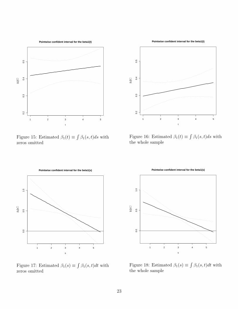
Figures 13 to 18 shows the estimated β1(s, t), β1(t) =∫β1(s, t)ds) and β1(s) =
∫β1(s, t)dt) including
and excluding the observations with zeros. If we compare the cases with and without the zeros, the
shape of the curves are similar, but there is a clear gain of using the whole sample in terms of efficiency.
Our approach also gives a more complete understanding of the correlation between fathers and sons.
If we look at Figure 13 or 14, for example, we see that the surface is declining in the direction of s,
the time dimension for fathers. It is therefore the father’s earnings in early stage of his life that is the
most correlated with son’s earnings. Figure 15 or 16 shows that the average effect over the son’s life is
increasing; figure 17 or 18 shows, however, that the correlation is declining with the father’s age and
this decline is significant.
5 Conclusion
In this paper, we extend the functional regression with functional response method of Ramsay and
Silverman (2005) to the case of multiple functional regressors. We also offer an alternative approach
when observations contains zeros and the data have to be expressed in logarithms. The Monte Carlo
experiment suggests that the method performs relatively well in comparison to OLS in terms of its
ability to identify the functional parameters. The simulation also shows that our way of dealing with
the zeros produces less biased and more efficient estimates. We then apply our method to measure
21

Model 1 Model 2 Model 3 Model 4Intercept 2.1101∗∗∗ 3.1659∗∗∗ 0.6145∗∗∗ 4.2966∗∗∗
(0.6019) (0.0915) (0.1750) (0.0932)F 0.4454∗∗∗ 0.4470∗∗∗ 0.3479∗∗∗ 0.3357∗∗∗
(0.0315) (0.0310) (0.0257) (0.0254)FA −0.0029 −0.0080∗∗ 0.0113∗ −0.0033
(0.0280) (0.0028) (0.0054) (0.0029)SA 0.0129 0.0322∗∗∗ 0.0545∗∗ 0.0216∗
(0.0398) (0.0084) (0.0187) (0.0091)FA2 0.0001 −0.0007∗
(0.0003) (0.0003)SA2 −0.0013 −0.0048∗∗∗
(0.0031) (0.0015)Cross-Val. 501.4828 495.5293 1397.5486 1288.7777Num. obs. 254 254 297 297∗∗∗p < 0.001, ∗∗p < 0.01, ∗p < 0.05
Table 6: Functional regression estimates of the intergenerational mobility
Confidence surface for beta1(s,t)
1
2
3
4
5
1
2
3
4
5
−0.1
0.0
0.1
0.2
0.3
st
z
−0.1
0.0
0.1
0.2
0.3
Figure 13: Estimated β1(s, t) with zeros omit-ted
Confidence surface for beta1(s,t)
1
2
3
4
5
1
2
3
4
5
−0.1
0.0
0.1
0.2
0.3
st
z
−0.10
−0.05
0.00
0.05
0.10
0.15
0.20
0.25
Figure 14: Estimated β1(s, t) with the wholesample
22
1 2 3 4 5
0.2
0.3
0.4
0.5
t
β 1(t)
Pointwise confident interval for the beta1(t)
Figure 15: Estimated β1(t) ≡∫β1(s, t)ds with
zeros omitted
1 2 3 4 5
0.2
0.3
0.4
0.5
t
β 1(t)
Pointwise confident interval for the beta1(t)
Figure 16: Estimated β1(t) ≡∫β1(s, t)ds with
the whole sample
1 2 3 4 5
0.0
0.5
1.0
s
β 1(s
)
Pointwise confident interval for the beta1(s)
Figure 17: Estimated β1(s) ≡∫β1(s, t)dt with
zeros omitted
1 2 3 4 5
0.0
0.5
1.0
s
β 1(s
)
Pointwise confident interval for the beta1(s)
Figure 18: Estimated β1(s) ≡∫β1(s, t)dt with
the whole sample
23

intergenerational mobility using a panel from the PSID. The method offers a way to better analyze
the elasticity between fathers’ earnings at any point in time and sons’s earnings. It also offers a non-
parametric and data-driven method for dealing with the zeros instead of simply replacing them with an
arbitrary value. The elasticity that we estimate is located between the one obtained by Solon (1992)
and Haider and Solon (2006) an the one obtain by Couch and Lillard (1998).
24

References
Yacine Aıt-Sahalia. Maximum likelihood estimation of discretely sampled diffusions: A closed-form
approximation approach. Econometrica, 70(1):223–262, 2002.
J.S. Altonji and T. Dunn. Relationships among the family incomes and labor market outcomes of
relatives. Research in Labor Economics, 12:269–310, 1991.
G.S. Becker and N. Tomes. Human capital and the rise and fall of families. In Gary S. Becker, editor,
Human Capital: A Theoretical and Empirical Analysis with Special Reference to Education. Chicago
Press, Chicago, IL, 1986.
T. Chen and K.A. Couch. An approximation of logarithmic functions in the regression setting. Statistical
Methodology, 23:50–58, 2015.
T. Chen and Q. Fan. A functional data approach to model score difference process in professional
basketball games. Journal of Applied Statistics, forthcoming.
K.A. Couch and D.R. Lillard. Sample selection and the intergenerational correlation in earnings. Labour
Economics, 5:313–329, 1998.
K.A. Couch, M.C. Daly, and D.A. Wolf. Time? money? both? the allocation of ressources to older
parents. Demography, 36(2):219–232, 1999.
R.B. Freeman. Black economic progress after 1964: Who has gained and why? In S. Rosen, editor,
Studies in Labor Market. University of Chicago Press, Chicago, 1981.
S. Haider and G. Solon. Life-cycle variation in the association between current and lifetime earnings.
American Economic Review, 96(4):1308–1320, 2006.
T. Lancaster. The incidental parameter problem since 1948. Journal of Econometrics, 95:391–413, 2000.
25

A. Laukaitis. Functional data analyisis for cash flow and transactions intensity continuouts-time predic-
tion using hilbert-valued autoregressive processes. European Journal of Operation Research, 185(3):
1607–1614, 2008.
S. Lopez-Pintado and J. Romo. On the concept of depth for functional data. Journal of the American
Statistical Association, 104(486):718–734, 2009. doi: 10.1198/jasa.2009.0108.
Robert C Merton. On estimating the expected return on the market: An exploratory investigation.
Journal of Financial Economics, 8(4):323–361, 1980.
J.O. Ramsay and C.J. Dalzell. Some tools for functional data analysis (with discussion). Journal of the
Royal Statistical Society, 53:539–572, 1991.
J.O. Ramsay and J.B. Ramsey. Functional data analysis of the dynamics of the monthly index of
nondurable goods production. Journal of Econometrics, 107(1-2):327–344, 2002.
J.O. Ramsay and B.W. Silverman. Functional data analysis. Springer, 2005.
G. Solon. Intergenerational income mobility in the united states. American Economic Review, 82:
393–408, 1992.
A. Sood, G. James, and Tellis G. Functional regression: A new model for predicing marekt penetration
of new products. Marketing Science, 28(1):36–51, 2009.
Y. Sun and M.G. Genton. Functional boxplots. Journal of Computational and Graphical Statistics, 20
(2):316–334, 2011. doi: 10.1198/jcgs.2011.09224.
S. Wang, W. Jank, and Shmueli G. Explaning the forecasting online auction prices and their dynamics
uing functional data analysis. Journal of Busniess & Economic Statistics, 26(2):144–160, 2008.
S.J. Wright. Coordinate descent algorithms. Mathematical Programming, 151(1):3–34, 2015.
D.J. Zimmerman. Regression toward mediocrity in economic stature. Labour Economics, 82:409–429,
1992.
26
Appendix
A Derivation of the functional regression
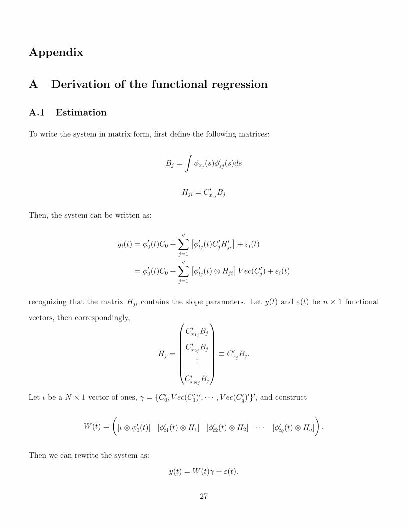
A.1 Estimation
To write the system in matrix form, first define the following matrices:
Bj =
∫φxj(s)φ
′sj(s)ds
Hji = C ′xijBj
Then, the system can be written as:
yi(t) = φ′0(t)C0 +
q∑j=1
[φ′tj(t)C
′jH′ji
]+ εi(t)
= φ′0(t)C0 +
q∑j=1
[φ′tj(t)⊗Hji
]V ec(C ′j) + εi(t)
recognizing that the matrix Hji contains the slope parameters. Let y(t) and ε(t) be n × 1 functional
vectors, then correspondingly,
Hj =
C ′x1jBj
C ′x2jBj
...
C ′xNjBj
≡ C ′xjBj.
Let ι be a N × 1 vector of ones, γ = C ′0, V ec(C ′1)′, · · · , V ec(C ′q)′′, and construct
W (t) =
([ι⊗ φ′0(t)] [φ′t1(t)⊗H1] [φ′t2(t)⊗H2] · · · [φ′tq(t)⊗Hq]
).
Then we can rewrite the system as:
y(t) = W (t)γ + ε(t).
27

The vector of coefficients γ can be estimated by minimizing the sum of squared errors plus a penalty
function:
SSE =
∫ε′(t)ε(t)dt+
q∑l=0
Pl,
where the penalties Pl are defined as:
P0 = λ0
∫(L0β0(t))2dt
for β0(t).
Pj = λsj
∫ ∫(Lsjβj(s, t))
2dsdt+ λtj
∫ ∫(Ltjβj(s, t))
2dsdt
for βj(s, t), where L0, Lsj and Ltj are linear differential operators. We can rewrite these penalties in
matrix form as follows:
P0 = λ0
∫(L0β0(t))2dt = λ0C
′0
[∫[L0φ0(t)][L0φ0(t)]′dt
]C0 = λ0[C ′0R0C0] ≡ C ′0R0(λ0)C0
To construct βj(s, t)’s penalty, define the following terms:
βjtt =
∫φj(t)φ
′j(t)dt,
βjss =
∫φj(s)φ
′j(s)ds,
Rsj =
∫[Lsjφsj(s)][Lsjφsj(s)]
′ds,
and
Rtj =
∫[Ltjφtj(t)][Ltjφtj(t)]
′dt.
28

Then
Pj = λsj
∫ ∫(Lsβj(s, t))
2dsdt+ λtj
∫ ∫(Ltβj(s, t))
2dsdt
= V ec(Cj)′λsj[Rsj ⊗ βjtt] + λtj[βjss ⊗Rtj]
V ec(Cj)
= V ec(Cj)′Rj(λsj, λtj)V ec(Cj)
The whole penalty term can therefore be written as:
q∑l=0
Pl = γ′R(λ)γ
where the bloc diagonal matrix R(λ) appears as
R(λ) =
R0(λ0) 0 0 · · · 0
0 R1(λ1s, λ1t) 0 · · · 0
......
.... . .
...
0 0 0 0 Rq(λqs, λqt)
.
We want to solve (the dependence of R on λ is removed for clarity)
γ = arg minγ
SSE =
∫y′(t)y(t)dt− 2γ′
[∫W ′(t)y(t)dt
]+ γ′
[∫W ′(t)W (t)dt+R
]γ.
The solution is:
γ =
[∫W ′(t)W (t)dt+R
]−1 [∫W ′(t)y(t)dt
].
29

The term [∫W ′(t)W (t)dt] can be computed as follows:
[∫W ′(t)W (t)dt
]11
=
∫[ι′ ⊗ φ0(t)][ι⊗ φ′0(t)]dt
=
∫[ι′ι⊗ φ0(t)φ′0(t)]dt
= N
∫φ0(t)φ′0(t)]dt,
[∫W ′(t)W (t)dt
]1j
=
∫[ι′ ⊗ φ0(t)][φ′tj(t)⊗Hj]dt
=
∫[ι′Hj ⊗ φ0(t)φ′tj(t)]dt
= [ι′Hj]
∫φ0(t)φ′tj(t)]dt for j > 1,
and
[∫W ′(t)W (t)dt
]ij
=
∫[φti(t)⊗H ′i][φ′tj(t)⊗Hj]dt
=
∫[H ′iHj ⊗ φti(t)φ′tj(t)]dt
= [H ′iHj]⊗∫φti(t)φ
′tj(t)dt for i, j > 1.
A.2 Construction of the confidence surfaces
In order to analyze the performance of our method, we construct functional confidence bands based
on the functions’ depth. In particular, we use the modified band depth measure (MBD) proposed by
Lopez-Pintado and Romo (2009). Depth measures allow to order functions and construct functional
box-plots as it is well described by Sun and Genton (2011). In particular, a functional box-plot allows
us to detect outliers among the estimated curves, which, in our case, may be a sign of convergence
30

1 2 3 4 5
−10
010
20
s
β 2(s
)
Figure 19: Functional Box-Plot for β2(s) usingall observations
1 2 3 4 5
−2
02
46
s
β 2(s
)
Figure 20: Functional Box-Plot for β2(s) afterre-estimating the outliers
problems while estimating the optimal smoothing parameters.
In the case of random functions, we can have magnitude or shape outliers. We are more likely to
encounter the latter when the smoothing parameters are not properly chosen as we can see in Figure 19.
In that case, 665 out of 5, 000 models were re-estimated because the smoothing parameters were clearly
too small, given the shape of the outliers. The result is shown in Figure 20.
A function depth is a measure of where the function stands with respect to the median curve. The
curve with the highest depth is therefore the median. The MBD measure is the point-wise proportion
that a curve lies between all pairs of curves. Although Sun and Genton (2011) only illustrate the case
of two-dimensional functions, it is straightforward to generalize it to functions with higher dimensions.
Once the depth measure is obtained for all curves, the 95% confidence band is obtained by computing
the sup and inf of 95% of all curves with the highest depth. Since we have 5, 000 replication in our
simulations, we computed the sup and the inf of the 4, 750 estimated curves with the highest depth.
31
Top Related