


Languages
Pages
Legal


Techniques of Water-Resources Investigations of the United States Geological Survey
CHAPTER Dl
APPLICATION OF SURFACE GEOPHYSICS TO GROUND-WATER INVESTIGATIONS
By A. A. R. Zohdy, G. P. Eaton, and D. R. Mabey
BOOK 2 COLLECTION OF ENVIRONMENTAL DATA

Magnetic .Methods By D. R. Mabey
The magnetic method of geophysical exploration involves measurements of the direction, gradient, or iatensity of the Earth’s magnetic field and interpretation of variations in these quantities over the area of investigation. Magnetic surveys can be made on the land surface, from an aircraft, or from a ship. Most exploration surveys made today measure either the relative or absolute intensity of the total field or the vertical component. Measurements of magnetic in-tensity can ,bemade with silmple mechanical balances or with elaborate electronic instruments.
The unit of magnetic intensity used almost exclusively in exploration geophysics is a gamma(y~ A gamma is defined as lo-” oersted ; an oersted is the magnetic intensity at a point that will exert a force of 1 dyne on a unit magnetic pole. The intensity of the magnetic field on or above the surface of the Earthis dependent upon the location of the observation point in the primary magnetic field of the Earth and local or regional concentrations of magnetic material. The in-tensity of the Earth’s undisturbed magnetic field ranges from a mini,mum of about 26,000 y at the magnetic equator to more than 69,600 y near the magnetic poles. Over the United ‘States,exclusive of Hawaii, the range is from 49,000,to 60,000y.
Magnetic anomalies are distor,tions of the magnetic field produced by magnetic material in the Earth’s crust or Iperhapsupper mantle. Magnetic anomalies of geologic interest are of two types: induced anomalies and remanent anomalies. Induced anomalies are the result of magnetization iaduced in a body by the Earth’s magnetic field. The anomaly produced is dependent upon the geometry,
orientation, and magnetic properties of the body, and the direction and intensity of the Earth’s field. Because of the dependence on the direction of the Earth’s field, magnetic anomalies produced by similar bodies may differ widely with geographic location. Remanent anomalies are the result of “permanent” magnetization of a #bodyand are controlled by the direction and mtensity of remanent magnetization and the geometry of the disturbing mass. Most magnetic anomalies are a combination of the two types, but usually one type of magnetization is dominant and the other can be ignored in the approximate interpretation of results.
Several types of information can be obtained from ‘magnetic surveys. The character of a magnetic anomaly is often indicative of the type of rock producing the anomaly, and an experienced interpreter can identify a general rock type on the basis of character of the magnetic anomalies observed. Quantitative interpretation of individjual magnetic anomalies yields information on the depth of burial, extent, structure, and magnetic properties of rock units. The most common use of magnetic data in ground-water studies is to map the depth to the magnetic basement rock.
Sedimentary frocks are the most common aquifers. However, most .sedimentary rocks are essentially nonmagnetic and thus not amenable to direct study by magnetic methods. A few elastic rocks, such as somestream deposits and beach sands, do contain magnetic minerals and can be studied directly.
1,gneousand metamorphic ‘rocks generally contain a larger proportion of magnetic minerals and are therefore more magnetic than sedimentary rocks but of less interest in
107

108 TE-CHNIQUES OF WATER-RESOURCES INVESTIGATIONS
ground-water investigations ; however, de-termination of the configuration of the surface of a basement complex composed of igneous and metamorphic rock underlying water-bearing sediments is important ,in nearby ground-water studies. In general the darker, more basic, rocks are more magnetic than the light colored, acidic mks. Some volcanic rocks, particu,larly basalts in the northwestern United States, are important aquifers.
Magnetic Surveys
Magnetic surveys may be very simple or very camplex, depending on the objectives of the survey. The ,amplitude of magnetic anomalies range from less than 1 7 to several thousand gammas ; horizontally the extent of these anomalies ranges from less than 1 m to tens of kilometers. The anomalies of larger am.plitude can be defined with simple instruments and procedures ; the small anomalies may require complex ones.
The simplest instruments for measuring magnetic ,intensi;ty involve balancing the force exerted by the vertical component of the Earth’s magnetic field on a magnet against the force of gravity. The simplest of these instruments, the dip needle, can be used to map the location of anomalies with amplitudes of several hundred gammas. With the Schmidt-type vertical balance, sensitivity of a few gammas can be obtained. Torsion instruments of comparable sensitivity also are available. Most types of mechanical instruments used to measure magnetic intensity are aim,ple to operate and, if protected from mechanical damage, are trouble free. Cenerally, the higher the sensitivity of a mechanical instrument for measuring magnetic intensity, the more care and time required to orient the instrument and complete an observation.
Several nonmechanical methods for measuring magnetic intensity are in common use. The fluxgate (magnetic saturation) magnetometers can be made sensitive to less than 1 7, but most handheld uni&&shave sensitiv-
0 ities of a few tens of gamlma63. Proton-precession magnetometers range in sensitivity from less than 1 gamma to a few gammas. Optical-absorption magnetometers are capable of measuring magnetic fields to 0.01 y. All these instruments can be adapted for use on a moving platform, and pairs of the optical-absorption magnetometers can be used to measure gradients.
The design of a magnetic survey is based on -the character of the magnetic anomalies expected and the type of interpretation to be made of the magnetic data. Airborne magnetic surveys measuring variations in the total magnetic intensity are the most common methods of obtaining magnetic data. To minimize magnetic disturbances from the aircraft, the magnetic sensor normally is towed from the aircraft or mounted in a boom extending from the aircraft,. Magnetic data are obtained continuously along a flight path. Although low-level flights may be prohibited in populated areas, ‘access is usually not a major problem in airborne surveys. Continuous magnetic measurements also can be made from a motor vehicle or boat if the sensor can *be located ,a few feet from the parto of the vehicle con,t..aining large masses of iron.
Time vari,ations in the magnetic field, which m,ust be corrected for, are important in some su,rveys. Secular variations are long term changes and usually can be ignored, but in special situations must .be considered. Of much greater importance are var,iations with a period of a day or less and with amplitudes ranging from less than 50 y for a :normal day to 1,000 y in high latitudes durin,g magnetic storms. A correction for solar diurnal variations with an average range of about 30 y usually can be made by repeated observations of a magnetometer station or profile dur,ing a surveying day. If accuracy of a few gammas or less is to be obtained, a continuous record of the magnetic variations at a location within or near the survey iarea is required.
For most exploration purposes it is only necessary to measure relative magnetic in-

APPLICATION OF SURFACE GEOPHYSICS 109
tensity over the area of interest. Thus, an arbitrary magnetic datum can be used for each map or profile.
Magnetic Properties
The magnetic susceptibility and remanent magnetization of rocks are the properties of interest in magnetic surveys. Susceptibility is a measure of the ability of a rock to acquire a magnetization in the presence of a magnetic field. Remanent magnetization is the permanent magnetization of rock and is not dependent on any contemporary external field. The ,ratio of the remanent magnetiza tion to induced magnetization is the Q ratio.
Induced magnetization i,s defined by the formula M = KH, x 10-S where K is the susceptibility in cgs units and H,, is the in-tensity of the applied field in gammas. Susceptibility of a rock is primarily dependent upon the composition and internal structure of the rock. The magnetic susceptibility of most rocks depends primarily on the content of magnetite and pyrrhotite, the two most common magnetic minerals.
Although remanent magnetization can be acquired by a rock in several ways, thermoremanent magnetization is the most important type. As an igneous rock cools through the Curie temperature (585°C for magnetite), it acquires a magnetization parallel to the Earth’s field. This thermoremanent magnetization is usually stable and remains with the rock through subsequent changes Yn the direction of the E,arth’s field. Most volcanic rocks are magnetic and many have
surface volcanic rocks the magnetic intensity may vary widely over short distances, and detai,led observations are ‘required to define the magnetic field near the surface. Although in many places the presence of volcanic rocks can be, inferred from the character of the magnetic field, the geologic significance of many of the very local magnetic features over volcanic rocks is not determined easily.
Design of Magnetic Surveys
The precision of the measurements, the detail obtained, and, with airborne surveya, the flight level, determine the cast of the survey as well as the usefulness of the data. Ideally a magnetic survey should define the major features of the magnetic field at a level which will resolve all anomalies of interest; however, the cost of obtaining this detail may be prohibitive. A more reahstic objective in areas of complex geology is to obtain sufficient data to resolve the major geologic uncertainties. Where rock type is to be determined, a survey that indicates the general character of the field without defining individual anomalies m’ay be adequate, and where approximate depth to basement rock is to be determined, gradients along profiles may be adequate data.
Detailed data along a single profile may be more useful than i,solated observations distributed over the entire area of interest be-cause most quantitative magnetic interpretation methods involve analysis of details of a m’agnetic anomaly (such as the extent of a uniform gradient, location of inflection points, 01’the position or amplitude of highs or lows).
Planning a magnetic survey involves three major decisions : 1. Can the data be best obtained by a ground
or airborne survey? For all except extremely detailed work, moat geophysicists prefer airborne data to ground data. However, the minimum cost of an airborne survey may be prohibitive.
2. What precision Is required? This determination will be based on the nature of the anomalies anticipated and the methods of interpretation to be at-tempted. For a ground survey this will determine the selection of a magnetometer, and the method used to correct for diurnal magnetic variations. Most magnetometers used in airborne surveys are capable of sufficient precision for most needs. However, if anomalies

110 TECHNIQUES OF WATER-RESOURCES INVESTIGATIONS 0
of very small amphtude are significant, map. T.herefore, profiles commonly are used the use of an optical-absorption mag- in making detailed interpretations. netometer may lberequired.
3. What detail is required? This consideration will govern the station spacing for ground surveys and the fli,ghtline spacing and flying height for &borne surveys. The problems relating to detail are discussed in the section on interpretation.
Data Reduction The reduction of magnetic data is rela
tively simple. Proton-precession and optical-absorption magnetometers measure the absolute value of the E,arth’s field. Other magnetometers provide a relative measure. The readings from the latter may be ‘in gammas or may require adjustment by a scale factor. Ground magnetometers generally are referenced to a base station or a stationary magnetometer. If a ,base magnetometer is operated, the difference between the ‘reading of the base magnetometer and the survey magnetometer at the observation time multiplied by the appropriate calibration constants will be the value <for the station. If repeat readinlgs at a base station are used as the method for determining diurnal variations, enough repeat readings must be obtained to construct a curve showing the variations of magnetic intensity with time.
In most airborne surveys, continuous or nearly continuous observations are made. The data are recorded on a paper chart or magnetic tape. The flight path of the air-craft is recorded in some manner, most commonly by photographing the path or by electronic navigation systems. The flight path is plotted and the data adjusted for variation in aircraft speed, instrument drift, and diurnal magnetic variations.
Magnetic data can be presented in profile form or as contour maps. Although magnetic contours ,provide an effective way of illustrating many magnetic features, some of the information that is available on continuous profiles cannot be illustrated on a contour
Interpretation of Magnetic. Data
The magnetization of most major *rock units is complex and the details*of the magnetic anomalies ‘are also complex. This, coupled wlith the inherent ambiguity, ,makes the comprehensive Werpretation of magnetic anomalies a com’plex art.
The two major aapplications of magnetic surveys to ,ground-water studies have been the study of magnetic aquifers, mainly basalIt, and the determination of the configuration of the basement rook ulnderlying the water-bearing sediments. T,he study of magnetic aquifers involves the Bidentification of rock type and, in some studies, the determination of geometry and magnetic 1properties. The study of basement-rock configuration generally involves determining the depth to the surface of the basement at several points and perhaps contouring the depths, ,but may also include determining relief on the basement surface,such as displacement across a fault.
Major magnetic rock umts commonly produce magnetic snomalies with characteristics that can lbe identified and used to infer the presence or absence of the <rock.Volcanic rocks may produce high amplitude magnetic variations of very local extent. Negative magnetic anomalies produced by Ipermanent magnetization in a direction approximately opposite to the Earth’s magnetic field may be associated with volcanic rocks. Large igneous intrusives produce anomalies with a wide ,range of amplitudes, but generally of greater extent and leas complex ,than the anomalies associated with volcanic rocks,and often approach the theoretical anomaly produced by simple geometric forms. BMamorphic rocks may produce complex patterns and pronounced lineaments are common. Most sedimentary rocks are nonmagnetic, but magnetite-beariag sands and gravels are a notable exception.

APPLICATION OF SURFACE GEOPHYSICS 111
An experienced interpreter generally can identify rock type by inspection of the magnetic anomaliies; however, such an interpretation is necessarily subjective. Contacts be, tween units of differing magnetic properties can be identified on magnetic maps and pro-files or traced in the field by dip needle or simple magnetometer surveys.
To determine the thickness of nonrr agnetic sedimentary rock overlying a magnetic basement, we ,assume that an observed anomaly is produced by a magnetic mass ex-tending upward to the su,rface of the basement. Several features of such an anomaly, such as the extent of the steepest gradient and the distance between various identifiable points on the anomaly, are u,sed. Assumptions must be made concerning the geometry of the disturbing mass, but these assump,tions generally’ are not critical. No assumption need be made on the physical properties of the rocks involved. Several procedures are used in this type of interpretation, and it i,s beyond the scope of this report to describe the methods. Vacquier and others (1951) describe a widely used technique for determining depths from magnetic anomalies and also illustrate a variety of anomalies. As a generalization, the closer the level of observations to a disturbing mass, the steeper the magnetic gradients and the smaller the extent of major features on the anomaly.
Under optimum conditions depth estimates made by a skilled interpreter are within 10 to 20 percent of the actual depths, and, in many sedimentary basins, good contour maps on the basement surface have been prepared from magnetic data. Aeromagnetic surveys have proven especially effective and valuable in reconnaissance su.rveys of sedimentary basins where large areas must be explored quiickly and where access on the surface is a problem. In some basins the sedimentary rock thicknesses obtained from magnetic data are more reliable than can be obtained by ‘any other geophysical method.
The ambiguities in,herent in the interpretation of magnetic data limit the extent to which the magnetic data can be -used to infer
the geometry of a disturbing mass. However, if detailed magnetic data are ,available, curve-matching techniques can be used effectively in identifymg simple geometric forms that could produce an observed anomaly. The character of many magnetic anomalies will indicate ,the form and the attitude of the ‘disturbing mass. For example, the anomaly produced by steeply dipping tabular bodies can be identified as reflecting a tabul,ar body, and, by assuming the direction of magnetization (generally parallel to the Earth’s magnetic field), the position, strike, and approximate dip of the body can be inferred. In some situations the width and magnetic properties also can be inferred. Bodies of more complex geometry are also amenable to modeling or curve matching, but as the geometric complexity increases, the uncertainties of the interpretation become greater. In most curve-matching or modeling procedures,uniform magnetization of the disturbing mass, as well as the enclosing material,is assu,med.For large bodies this assumption may not be justified,and the resulting interpretation #issulbject to large errors.
Some magnetic anomalies reflect variation in thickness or surface elevation of a magnetic unit. Computations of these thickness or elevation changes require the assumption of magnetic properties. Thus, the location of these features may be ,inferred, but the thickness or relief may be uncertain if information is not available on the magnetic properties.
Albumis of computed magnetic anomalies for masses of simple geometry and magnetization are being produced. Probably the best albums currently available are Vacquier and others (1951) and Andreasen and Zietz (1969).
Examples of Magnetic Surveys
Gem Valley, Idaho
Magnetic surveys have been used in the study of ,basallt aqmfers in several areas,
112 TECHNIQUES OF WATER-RE.SOURCES INVESTIGATIONS
particularly in the Snake River Plain and Colu’mbi,a Plateau, with varying degrees of success. Magnetic data from Gem Valley in southeastern Idaho illustrate some of the potentials and limitations of magnetic surveys in the study of volcanic rocks (Mabey and Oriel, 1970).
Gem Valley is an intermontane basin about 56 km (35 miles) long and as much as 13 km ‘(8 miles) wide. The enclosing ranges are Paleozoic sedi’mentary rocks. Much of the valley floor consists of Cenozoic basalt flows f,rom vents in the southeastern part of the valley and from an extensive volcanic field northeast of the valley. The ‘basalt flows in-undated a surface of unknown relief on the older Cenozoi< sediments. Post-basalt sediments overlap the basalt in several areas but sin most of the valley the basalt is over-lain by a thi,n cover of windblown soil. Water is pumped from basalt in several parts of the valley and infor,mation on the extent, thickness, and structure of the ,&salt is important to ground-water investigations in the valley.
Tlhe first magnetic observations in the valley consisted of measurements with a magnetometer moun,ted on a l-m tripod. The magnetic field in areas where the basalt was within a few feet of the surface varied several ‘hundred gammias over distances of a few meters. These abrupt variations reflect the magnetization of the upper few meters of the basalt and were of little value in determining the thickness or gross structure of the flows, so the survey was abandoned. The method could have been used to locate the edge of the Ibasalt where it was at shallow depths.
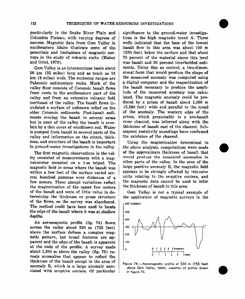
An aeromagnetic profile (fig. 74) flown across the valley about 230 m (755 feet) above the surface defines a complex magnetic pattern, but broad features are apparent and the edge of the ‘basalt is apparent at the ends *of the ‘prolYe. A survey made about 1,200 m above the valley (fig. 75) reveals anomahes that ‘appear to reflect the thickness of the basalt except in the area of anomaly B, which is a <large anomaly associated with eruptive centers. Of particular
0
significance to the ground-water investigations is the high magnetic trend. A. Three wells indicated that the base of the lowest basalt flow in this area was about 100 m (330 feet) below the surface and that about 70 percent of the material above this level was basalt and 30 percent interbedded sediments. Using this as control, a twodimensional form that would produce the shape of the measured anomaly was computed using a digital com,puter and the Imagnetization of the basalt necessary to produce the amplitude of the measured anomaly was calculated. T’he magnetic anomaly could be produced by a prism of ,basalt about 1,000 m (3,300 feet) wide and parallel to the trend of the anomaly. The western edge of the prism, which presumably is a prebasalt river channel, was inferred along with the thickness of ,basalt east of the channel. Sub-sequent resistivity soundings have confirmed the existence of the channel.
Using the magnetization determined in the above analysis, computations were made of the approximate thickness of basalt that would produce the measured anomalies in other parts of the valley. In the area of the large positive anomaly B, the ma.gnetic field appears to be strongly ~affeotedby intrusive units relating to the eruptive centers, and the magnetic data cannot be used to infer the thickness of basah in this area..
Gem Valley is not a tylpical example of the apphcation of magnetic surveys in the
T 600 GAMMAS
500t
Figure 74.-Aeromognetic profile at 230 m (755 feet) obove Gem Valley, Idoho. Location of profile shown in figure 75.

APPLICATION OF SURFACE GEOPHYSICS 113
study of volcanic aquifer problems, but it does illustrate some of the possible applications and limitations: (1) Magnetic surveys generally are effective in detecting and determining the extent of concealed volcanic rocks, and the approximate depth of burial of the volcanic rock can be inferred; and (2) quantitative interpretations of the thickness and ‘structure of volcanic rock can be mlade in ‘some simple situations, but generally cannot be made where a thick sequence of flows occurs or where the volcanic rocks are underlain by strongly magnetic rocks.
Antelope Valley, California If a sedimentary basin is underlain by
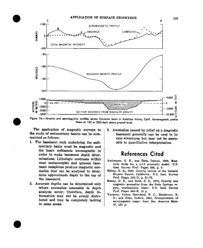
magnetic basement rock, magnetic surveys may be an effective tool in studying the structure of the basin. An example of this application of magnetic measurements is an aeromagnetic profile in eastern Antelope Val-ley, Calif. (fig. 76). The basement in this part of Antelope Valley is igneous rock of approximately quartz monzonite com,position. A Cenozoic basin several thousand feet deep has been defined by drilling and gravity measurements on the south side of Rosamond Lake (Mabey, 1960). Figure 76 illustrates the aeromagnetic and gravity profiles across the basin, and the configuration inferred from the gravity data and one deep drill hole (not along the profile) that did not penetrate the basement rock.
On the southern half of the profile are three local magnetic anomalies produced by lithologic variations in the basement rock. The character of these anomalies, which is better revealed on a contour map, is typical of anomalies over quartz monzonite in this part of the Mojave Desert. A skilled interpreter would infer from these anomalies that the rock producing the anomalies ,is similar to the quartz monzonite exposed a few miles to the east. Depths determined for sources of anomalies A and B were used to supplement the gravity data as control for the base of basin fill along the southern part of the profile. This interpretation involved assumptions on the geometry of the disturba
ing mass, which were not critical, and the assumption that the top of the disturbing mass extended to the top of the basement. However, because the determination of depths from these magnetic anom,alies does not involve assumptions of physical proper-ties or the removal of a regional gradient as do the gravity data, the magnetic depths for this part of the profile are more reliable than the depths determined from the gravity data. The magnetic data provide only two depths and do not provide a continuous indication of the depth to basement along the profile.
Near the north end of the profile is a double-peaked magnetic high. The extent of the gradients on this h,igh indicate an elevation of the top of the magnetic mass consistent with the elevation of the basement surface inferred from the gravity. The contrast in character between this anomaly and the anomalies at the south end of the profile suggests a difference in magnetic properties of the rock producing the anomalies, although all the anomalies probably are produced by intrusive rocks.
The magnetic low near the center of the profile is over the deepest part of the basin, but the lowest value is produced by the steeply dipping interface, probably a fault on the south side of the basin. The location of the fault and also a crude approximation of the vertical displacement could be inferred from the magnetic anomaly. Over the deepest part of the basin no local magnetic anomalies suitable for precise depth analysis were re-corded; therefore, the thickness of the basin fill in this area could not be determined from the magnetic data. Variations in the general level of magnetic intensity over the central and southern part of the profile, computed assuming a susceptibility contrast of 1.7~10.~ cgs units, agree with the measured intensity. Along most of the southern part of the profile the computed intensity is higher than the measured level, suggesting that the rock underlying this area has a lower susceptibility than the rock to the south.
114 TECHNIQUES OF WATER-RESOURCES INVESTIGATIONS
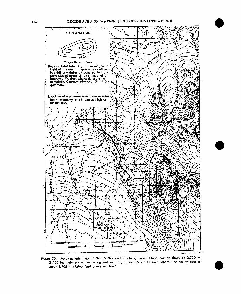
EXPLANATION’ y’ uLR \“’,
Magnetic contours ’ Showing total intensity of the magnetic
field of the earth in gammas relative to arbitrary datum. Hachured to indicate closed areas of lower magneticintensity. Dashed where data are in-
F complete. Contour intervals IO and 50 P’ gammas.
- Location of measured maximum or minimum intensity within closed high or
_ closed law.
Figure 75.-Aeromodnetic mop of Gem Volley ond adjoining oreos, Idaho. Survey flown at 2,700 m (8,900 feet) above seo level along eost-west flightlines 1.6 km (1 mile) apart. The volley floor is about 1,700 m (5,600 feet) obove sea level.
APPLICATION OF SURFACE GEOPHYSICS 116 5 N
+I00 r AEROMAGNETIC PROFILE .
. .
2 0 z
d
TOTAL MAGNETIC INTENSITY
-100
-90
Ted -100
s3dI -110
-120 c
Figure 76.-Gravity and aeromagnetic profiles across Cenozoic basin in Antelope Volley, Colif. Aeromagnetic ptofze flown at 150 m (500 feet) above ground level.
The application of magnetic surveys to the study of sedimentary basins can be summarized as follows : 1. The basement rock underlying the sedi
mentary ‘basin must ibe magnetic and the ‘basin sedimen,ts nonmagnetic in order to make basement depth determinations. Lithologic contrasm within most metamorphic and igneous basement oontplexesproduce <magneticanomalies that can be analyzed to deter-mine approximate depth to the top of the basement.
2. Accurate depths can be determined only where anomalies amenable to de&h -A-“-J “..a -..A , “II”& “l”l b, 1
formation may not be evenIly distributed and may be complete1ly lacking in some areas.
3. Anomalies causedby relief on a magnetic basement generally can be used to locate structures but #maynot ,be amen-able to quantitative interpretation.
References Cited Andreasen,G. E., and Zietz, Lidore, 1969, Mag
netic fields for a 4X6 prismatic model: U.S. Geol. Survey Prof. Paper 666, p. 9.
Mabey, D. R., 1960, Gravity survey of the western Mojave Desert, California: U.S. Geol. Survey Prof. Paper 31&D, p. 61-73.
Mabey, D. R., and Oriel, S. S., 1970, Gravity and magnetic anomalies from the Soda Springs region, southeastern Idaho: U.S. Geol. Survey Prof. Paper 646-E, 16 p.
Vacquier, Victor, Steenland, N. C., Henderson, R. G., and Zietz, Isidore, 1951, Interpretation of aeromagnetic maps: Geol. Sot. America Mem. 47, 151 p.
Cost of Geophysical
Electrical Methods Deep resistivity surveys normally are
made with a g-man crew, equipment costi,ng between $5,000 and $10,000, and two vehicles. Two of the crew ,members should be technically trained, but the other positions require no special training. The major cost of the field operation is the salary and expenses of the crew. The average cost of one crew-month including preliminary data interpretation is about $10,000. Under normlal conditions in one month a crew could make about 50 soundings to a depth of 900 m (3,000 feet), 100 soundilngs to 150 m (500 feet), or 80 km (50 miles) of profiling to 150 m (500 feet).
The cost of induced-polarization surveys is somewhat greater than resistivity surveys. Electromagnetic surveys are usually less ex-pensive and the coverage may be more rapid.
Telluric and magneto-telluric surveys are generally experimental and generalizations on cost and coverage are not meaningful.
Grwi ty Surveys The cost of gravity surveying varies wide
ly, depending on the station density required, the accessibility of the stations, and the presence or absence of adequate elevation control. In detailed studies of near-surface effects, where the station spacing is measured in terms of hundreds of feet, the cost, exclusive of elevation surveying, can :be as low as $5 per station with the d,ata reduced and interpreted in preliminary fashion. If the elevation’s in such a study must be wtablished independently, ,the cost till be approximately double. At the other extreme, for widely scattered stations in mountainous or hilly terrain, where backpacking or helicopter support is required, the cost may rise to $25
116
Surveys in 1970
or $30 per station. The nature of the problem will dictate the required station spacing, at least approximately, and estimates of cost are best made after a preliminary assessment of ‘the problem, a study of the terrain, and a check on the avability of elevation control.
Seismic Surveys The cost of seismic refraction surveys, in
cluding interpretation, varies from $600 to $750 per linear mile of coverage, depending on the geophone spacin,g. Shallow soundings, with short geophone spacings, are the more expensive, but provide more detailed information than do deeper soundings. If the objective (for example, the basement surface) is as much as 3,000 m (10,000 feet) below the surface, geophone spreads several miles long will be required to defme the surface. The completed cost for a single depth determination may be as *much as $2,500 to $3,000. On the other hand, for a refractor at a depth of 300 m (1,000 feet), only a mile or so of shooting would be required for definition and the consequent cost would be somewhere in the neighborhood of $700.
Magnetic Surveys
Aeromagnetic surveys, which measure total magnetic intensity, normally cost be-tween $5 and $15 per flightline lmile depending ,primarily on the size of the area to be surveyed. This cost includes the preparation of a contour map and profiles along flight-lines. The major cost of a ground survey is the salary and expenses for the crew (one or two men) and transportation. Using electronic magnetometers, a magnetometer observation can be made in less than 1 minute.
Top Related