Download - Application of Spectroscopic Doppler Velocimetry … of Spectroscopic Doppler Velocimetry for ... Doppler Velocimetry and Fabry-Perot Interferometry ... Doppler effect due to the motion

Application of Spectroscopic Doppler Velocimetry for

Measurement of Streamwise Vorticity

Amy F. Fagan*, Khairul B.M.Q. Zaman

†

NASA Glenn Research Center, Cleveland, Ohio, 44135

Kristie A. Elam‡

Jacobs Sverdrup, Cleveland, OH 44135

Michelle M. Clem§

NASA Glenn Research Center, Cleveland, Ohio, 44135

A spectroscopic Doppler velocimetry technique has been developed for measuring two

transverse components of velocity and hence streamwise vorticity in free jet flows. The

nonintrusive optical measurement system uses Mie scattering from a 200 mW green

continuous-wave laser interacting with dust and other tracer particulates naturally present

in the air flow to measure the velocities. Scattered light is collected in two opposing

directions to provide measurements of two orthogonal velocity components. An air-spaced

Fabry-Perot interferometer is used for spectral analysis to determine the optical frequency

shift between the incident laser light and the Mie scattered light. This frequency shift is

directly proportional to the velocity component in the direction of the bisector of the incident

and scattered light wave propagation vectors. Data were acquired for jet Mach numbers of

1.73 and 0.99 using a convergent 1.27-cm diameter round nozzle fitted with a single

triangular “delta-tab”. The velocity components and the streamwise vorticity calculated

from the measurements are presented. The results demonstrate the ability of this novel

optical system to obtain velocity and vorticity data without any artificial seeding and using a

low power laser system.

Nomenclature

Ab = amplitude of broadband light (CCD greylevels)

Ar = amplitude of reference signal (CCD greylevels)

AM = amplitude of Mie signal (CCD greylevels)

c = speed of light (= 2.998 x 108 m s

-1)

Ce = speed of sound at the jet exit (m s-1

)

d = Fabry-Perot interferometer plate spacing (m)

D = jet exit diameter (m)

E = incident electric field vector (V m-1

)

f = focal length of a lens (m)

fC = collimating lens focal length (m)

fL = fringe forming lens focal length (m)

FSR = free spectral range of the Fabry-Perot interferometer (s-1

)

IFP = Fabry-Perot instrument function

K = interaction wave vector (m-1

)

K = magnitude of K (m-1

)

k0 = incident light wave vector (m-1

)

* Research Engineer, Optical Instrumentation and NDE Branch, 21000 Brookpark Road, AIAA Senior Member

† Research Engineer, Inlet and Nozzle Branch, 21000 Brookpark Road, AIAA Associate Fellow

‡ Optics Technician, 21000 Brookpark Road

§ Research Engineer, Optical Instrumentation and NDE Branch, 21000 Brookpark Road

https://ntrs.nasa.gov/search.jsp?R=20130010926 2018-06-26T11:28:33+00:00Z

American Institute of Aeronautics and Astronautics

2

ks = scattered light wave vector (m-1

)

Mj = fully-expanded Mach number

n0 = reference interference fringe order

Nq = photoelectron counts detected by qth

pixel

r = radial position in the detector plane (m)

RMie = radius of the Mie signal interference fringe (m)

Rref = radius of the reference signal interference fringe (m)

Uj = fully-expanded jet velocity (m s-1

)

v = velocity vector (m s-1

)

v = velocity component in the y-direction (m s-1

)

vk = measured velocity component along K direction (m s-1

)

w = velocity component in the z-direction (m s-1

)

x = axial location in the jet flow (m)

xi = horizontal position in image plane (m)

xq = horizontal position of the qth

pixel center (m)

y = vertical position in the jet flow (m)

yi = vertical position in image plane (m)

yq = vertical position of qth

pixel center (m)

z = horizontal location in the jet flow (m)

angle between E and scattering plane (rad)

p = width of square CCD pixel (m)

x = streamwise vorticity (rad s-1

)

= angle of the light ray passing through etalon (rad)

illumination wavelength (m)

= etalon cavity refractive index

= frequency of scattered light (s-1

)

0 = frequency of incident laser light (s-1

)

s scattering angle (rad)

I. Introduction

ANY non-intrusive velocimetry techniques exist that are mature and in wide use in aerodynamic research.

Among these are particle image velocimetry (PIV)1, laser Doppler velocimetry (LDV)

2, planar Doppler

velocimetry (PDV)3, and Rayleigh scattering

4. The instrumentation development that is the topic of this paper is an

extension of a spectroscopic Rayleigh scattering system that has been developed at NASA Glenn Research Center

(GRC)5, and similar work at NASA Langley Research Center

6, where a Fabry-Perot (FP) Interferometry system is

used to analyze the Doppler frequency shift of Mie scattered light, rather than Rayleigh scattered light, to determine

two orthogonal components of velocity. The Mie scattering utilized in this technique occurs from a laser beam

interacting with naturally existing “seed” in a nozzle flow in the form of dust, oil, or other particulates present in the

facility air supply and ambient air and potentially from moisture condensation in the mixing layer between the cold

core flow and the warm ambient air. A FP interferometer or etalon is a high resolution filter based on interference

phenomena which is used to resolve the spectrum of the light. A FP interferometer consists of two parallel planar

reflective plates or surfaces and is typically used in the imaging mode7 (constant spacing between reflective

surfaces) for spectroscopic Mie or Rayleigh scattering. An etalon may be air-spaced or consist of a solid transparent

optical material. The air-spaced FP interferometer is used in this work to allow adjustment of the fringe pattern

during testing. When light is imaged through the FP an interference pattern results which is a function of the

frequency spectrum of the light convolved with the instrument function of the FP. The FP instrument function is the

well-known Airy function. Model functions of the incident laser light and the Mie scattered light convolved with the

FP instrument function are fitted to the recorded interference patterns to evaluate the frequency shift between the

incident and scattered light and thereby provide velocity measurements.

The main advantage of using the Mie signal as opposed to the Rayleigh signal to obtain velocity measurements

in this spectroscopic technique is that the intensity of the Mie scattering is much greater than that of Rayleigh

scattering. Also, the Mie spectral peak is much narrower, allowing for more accurate velocity estimates. The

advantage of the technique over PIV, LDV, or PDV is that it requires very little, if any, artificial flow seeding. In

M


3

this experiment no artificial seeding was used; however, if one did have a need to induce artificial seeding to

increase signal levels, the required seeding density to obtain adequate signals would be much less than the amount

required for PIV, LDV, or PDV. The current system incorporates a relatively low power 200 mW continuous-wave

(cw) single-mode, frequency-stabilized, narrow linewidth green laser system as the incident light source. This

enabled mounting of the laser and collection optics entirely on a vertical framework to allow the probe volume to be

translated horizontally and vertically within a cross-sectional plane of the nozzle flow. The ability to measure two

components of velocity using a lower power cw laser system is also an advantage of this technique over PIV, PDV,

and Rayleigh scattering. The system was used to obtain v and w velocity components which then were used to

calculate vorticity in a cross-sectional plane of a 1.27-cm diameter nozzle flow at two different Mach numbers. The

nozzle was fitted with a single triangular “delta-tab” located at the top of the exit in order to generate a pair of

counter-rotating vortices in the flow field.

II. Doppler Velocimetry and Fabry-Perot Interferometry

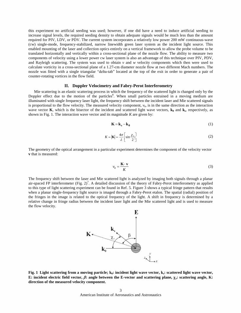
Mie scattering is an elastic scattering process in which the frequency of the scattered light is changed only by the

Doppler effect due to the motion of the particles8. When small particles entrained in a moving medium are

illuminated with single frequency laser light, the frequency shift between the incident laser and Mie scattered signals

is proportional to the flow velocity. The measured velocity component, vk, is in the same direction as the interaction

wave vector K, which is the bisector of the incident and scattered light wave vectors, k0 and ks, respectively, as

shown in Fig. 1. The interaction wave vector and its magnitude K are given by:

0s kkK (1)

2sin

4 sK

K (2)

The geometry of the optical arrangement in a particular experiment determines the component of the velocity vector

v that is measured:

K

vk

vK (3)

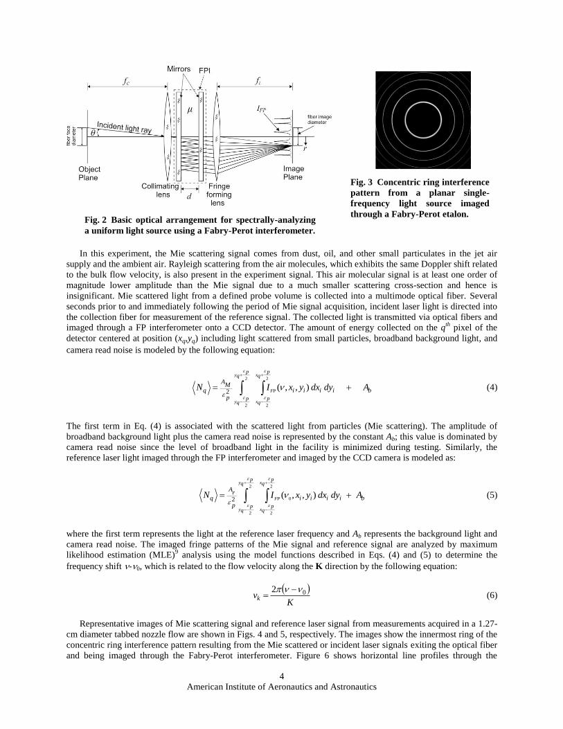
The frequency shift between the laser and Mie scattered light is analyzed by imaging both signals through a planar

air-spaced FP interferometer (Fig. 2)7. A detailed discussion of the theory of Fabry-Perot interferometry as applied

to this type of light scattering experiment can be found in Ref. 5. Figure 3 shows a typical fringe pattern that results

when a planar single-frequency light source is imaged through a Fabry-Perot etalon. The spatial (radial) position of

the fringes in the image is related to the optical frequency of the light. A shift in frequency is determined by a

relative change in fringe radius between the incident laser light and the Mie scattered light and is used to measure

the flow velocity.

Fig. 1 Light scattering from a moving particle; k0: incident light wave vector, ks: scattered light wave vector,

E: incident electric field vector, : angle between the E-vector and scattering plane, s: scattering angle, K:

direction of the measured velocity component.


4

In this experiment, the Mie scattering signal comes from dust, oil, and other small particulates in the jet air

supply and the ambient air. Rayleigh scattering from the air molecules, which exhibits the same Doppler shift related

to the bulk flow velocity, is also present in the experiment signal. This air molecular signal is at least one order of

magnitude lower amplitude than the Mie signal due to a much smaller scattering cross-section and hence is

insignificant. Mie scattered light from a defined probe volume is collected into a multimode optical fiber. Several

seconds prior to and immediately following the period of Mie signal acquisition, incident laser light is directed into

the collection fiber for measurement of the reference signal. The collected light is transmitted via optical fibers and

imaged through a FP interferometer onto a CCD detector. The amount of energy collected on the qth

pixel of the

detector centered at position (xq,yq) including light scattered from small particles, broadband background light, and

camera read noise is modeled by the following equation:

biiiip

MA

q AdydxyxIN

pq

pq

pq

pq

y

y

x

x

FP ),,(

2

2

2

2

2

(4)

The first term in Eq. (4) is associated with the scattered light from particles (Mie scattering). The amplitude of

broadband background light plus the camera read noise is represented by the constant Ab; this value is dominated by

camera read noise since the level of broadband light in the facility is minimized during testing. Similarly, the

reference laser light imaged through the FP interferometer and imaged by the CCD camera is modeled as:

biiiip

rA

q AdydxyxIN

pq

pq

pq

pq

y

y

x

x

FP ),,(

2

2

2

2

02

(5)

where the first term represents the light at the reference laser frequency and Ab represents the background light and

camera read noise. The imaged fringe patterns of the Mie signal and reference signal are analyzed by maximum

likelihood estimation (MLE)9 analysis using the model functions described in Eqs. (4) and (5) to determine the

frequency shift -0, which is related to the flow velocity along the K direction by the following equation:

Kvk

02 (6)

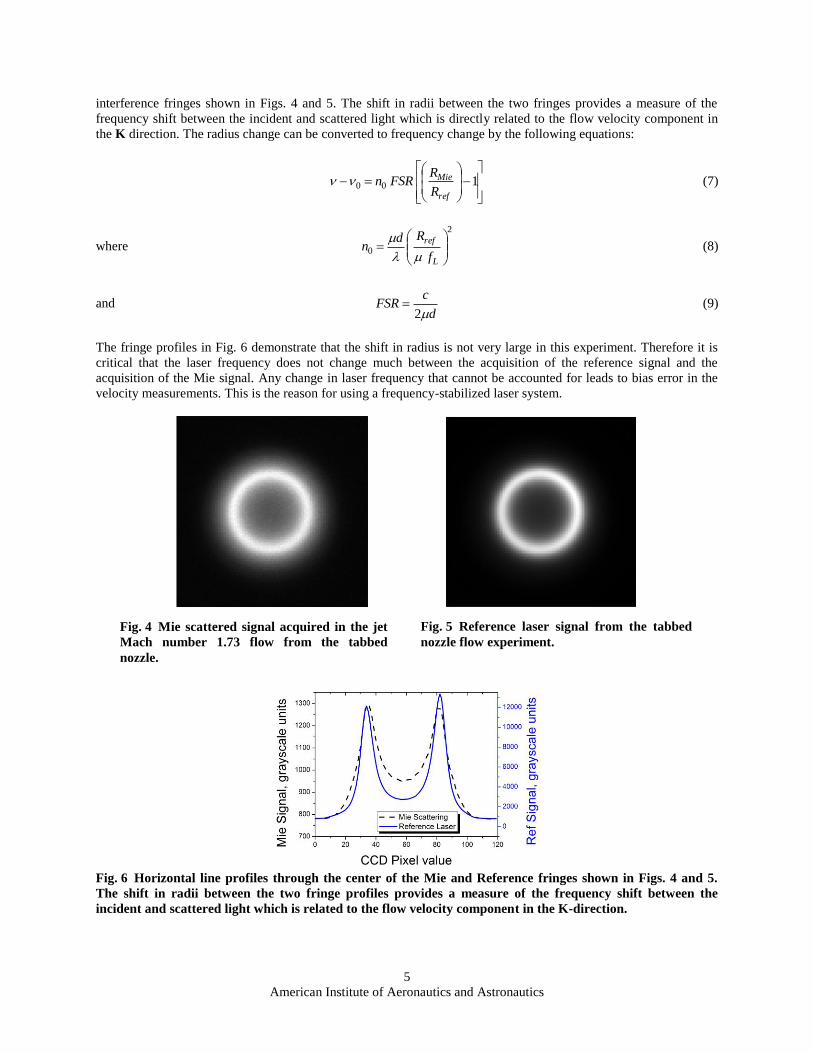
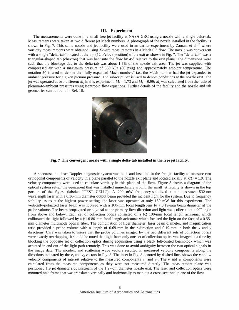
Representative images of Mie scattering signal and reference laser signal from measurements acquired in a 1.27-

cm diameter tabbed nozzle flow are shown in Figs. 4 and 5, respectively. The images show the innermost ring of the

concentric ring interference pattern resulting from the Mie scattered or incident laser signals exiting the optical fiber

and being imaged through the Fabry-Perot interferometer. Figure 6 shows horizontal line profiles through the

Fig. 2 Basic optical arrangement for spectrally-analyzing

a uniform light source using a Fabry-Perot interferometer.

Fig. 3 Concentric ring interference

pattern from a planar single-

frequency light source imaged

through a Fabry-Perot etalon.


5

interference fringes shown in Figs. 4 and 5. The shift in radii between the two fringes provides a measure of the

frequency shift between the incident and scattered light which is directly related to the flow velocity component in

the K direction. The radius change can be converted to frequency change by the following equations:

1 00

ref

Mie

R

RFSRn (7)

where

2

0

L

ref

f

Rdn

(8)

and d

cFSR

2 (9)

The fringe profiles in Fig. 6 demonstrate that the shift in radius is not very large in this experiment. Therefore it is

critical that the laser frequency does not change much between the acquisition of the reference signal and the

acquisition of the Mie signal. Any change in laser frequency that cannot be accounted for leads to bias error in the

velocity measurements. This is the reason for using a frequency-stabilized laser system.

Fig. 6 Horizontal line profiles through the center of the Mie and Reference fringes shown in Figs. 4 and 5.

The shift in radii between the two fringe profiles provides a measure of the frequency shift between the

incident and scattered light which is related to the flow velocity component in the K-direction.

Fig. 4 Mie scattered signal acquired in the jet

Mach number 1.73 flow from the tabbed

nozzle.

Fig. 5 Reference laser signal from the tabbed

nozzle flow experiment.


6

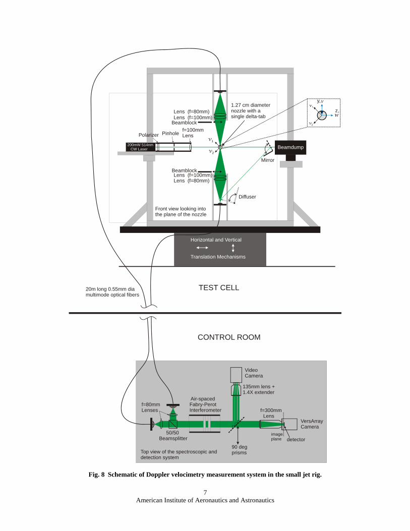
III. Experiment

The measurements were done in a small free jet facility at NASA GRC using a nozzle with a single delta-tab.

Measurements were taken at two different jet Mach numbers. A photograph of the nozzle installed in the facility is

shown in Fig. 7. This same nozzle and jet facility were used in an earlier experiment by Zaman, et al.10

where

vorticity measurements were obtained using X-wire measurements in a Mach 0.3 flow. The nozzle was convergent

with a single “delta-tab” located at the top (12 o‟clock position) of the exit as shown in Fig. 7. The “delta-tab” was a

triangular-shaped tab (chevron) that was bent into the flow by 45o relative to the exit plane. The dimensions were

such that the blockage due to the delta-tab was about 1.5% of the nozzle exit area. The jet was supplied with

compressed air with a maximum pressure of 560 kPa (80 psig) and approximately ambient temperature. The

notation Mj is used to denote the “fully expanded Mach number,” i.e., the Mach number had the jet expanded to

ambient pressure for a given plenum pressure. The subscript “e” is used to denote conditions at the nozzle exit. The

jet was operated at two different Mj in this experiment: Mj = 1.73 and Mj = 0.99; Mj was calculated from the ratio of

plenum-to-ambient pressures using isentropic flow equations. Further details of the facility and the nozzle and tab

geometries can be found in Ref. 10.

Fig. 7 The convergent nozzle with a single delta-tab installed in the free jet facility.

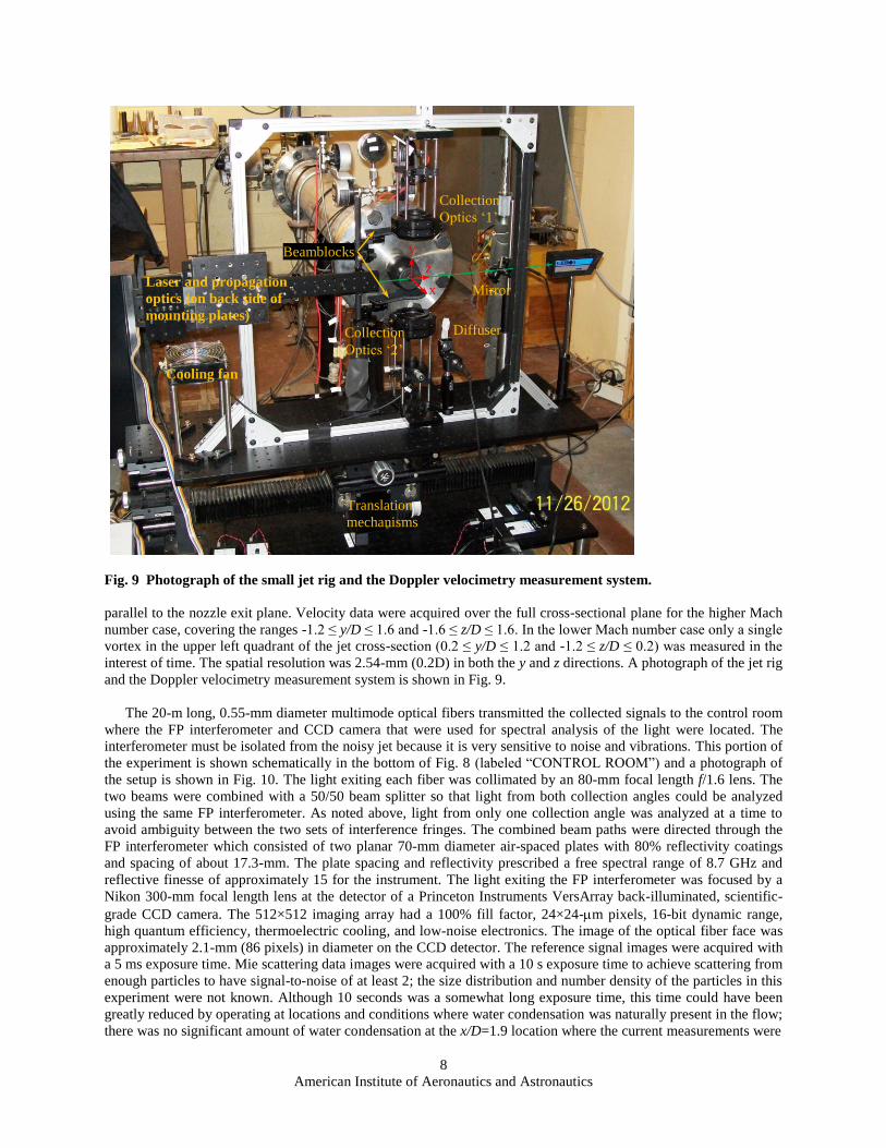
A spectroscopic laser Doppler diagnostic system was built and installed in the free jet facility to measure two

orthogonal components of velocity in a plane parallel to the nozzle exit plane and located axially at x/D = 1.9. The

velocity components were used to calculate vorticity in this plane of the flow. Figure 8 shows a diagram of the

optical system setup; the equipment that was installed immediately around the small jet facility is shown in the top

portion of the figure (labeled “TEST CELL”). A 200 mW frequency-stabilized continuous-wave 532-nm

wavelength laser with a 0.36-mm diameter output beam provided the incident light for the system. Due to frequency

stability issues at the highest power setting, the laser was operated at only 150 mW for this experiment. The

vertically-polarized laser beam was focused with a 100-mm focal length lens to a 0.19-mm beam diameter at the

probe volume. The beam propagated orthogonal to the primary flow direction and light was collected at a 90o angle

from above and below. Each set of collection optics consisted of a f/2 100-mm focal length achromat which

collimated the light followed by a f/1.6 80-mm focal length achromat which focused the light on the face of a 0.55-

mm diameter multimode optical fiber. The combination of fiber diameter, laser beam diameter, and magnification

ratio provided a probe volume with a length of 0.69-mm in the z-direction and 0.19-mm in both the x and y

directions. Care was taken to insure that the probe volumes imaged by the two different sets of collection optics

were exactly overlapping. It should be noted that light from only one set of collection optics was imaged at a time by

blocking the opposite set of collection optics during acquisition using a black felt-coated beamblock which was

actuated in and out of the light path remotely. This was done to avoid ambiguity between the two optical signals in

the image data. The incident and scattering wave vectors resulted in measured velocity components along the

directions indicated by the v1 and v2 vectors in Fig. 8. The inset in Fig. 8 denoted by dashed lines shows the v and w

velocity components of interest relative to the measured components v1 and v2. The v and w components were

calculated from the measured components as they were not measured directly. The measurement plane was

positioned 1.9 jet diameters downstream of the 1.27-cm diameter nozzle exit. The laser and collection optics were

mounted on a frame that was translated vertically and horizontally to map out a cross-sectional plane of the flow


7

VersArray Camera

f=80mm Lenses f=300mm

Lens

detectorimageplane

Air-spaced Fabry-Perot Interferometer

50/50 Beamsplitter

f=100mmLens

200mW 514nm CW Laser Beamdump

20m long 0.55mm diamultimode optical fibers

v1

v2

Lens (f=80mm)Lens (f=100mm)

Lens (f=100mm)Lens (f=80mm)

1.27 cm diameter nozzle with a single delta-tab

Front view looking intothe plane of the nozzle

Top view of the spectroscopic and detection system

Polarizer Pinhole

Beamblock

Beamblock

Diffuser

Mirror

90 degprisms

Video Camera

135mm lens + 1.4X extender

TEST CELL

CONTROL ROOM

Horizontal and Vertical

Translation Mechanisms

y,

z,

Fig. 8 Schematic of Doppler velocimetry measurement system in the small jet rig.


8

parallel to the nozzle exit plane. Velocity data were acquired over the full cross-sectional plane for the higher Mach

number case, covering the ranges -1.2 ≤ y/D ≤ 1.6 and -1.6 ≤ z/D ≤ 1.6. In the lower Mach number case only a single

vortex in the upper left quadrant of the jet cross-section (0.2 ≤ y/D ≤ 1.2 and -1.2 ≤ z/D ≤ 0.2) was measured in the

interest of time. The spatial resolution was 2.54-mm (0.2D) in both the y and z directions. A photograph of the jet rig

and the Doppler velocimetry measurement system is shown in Fig. 9.

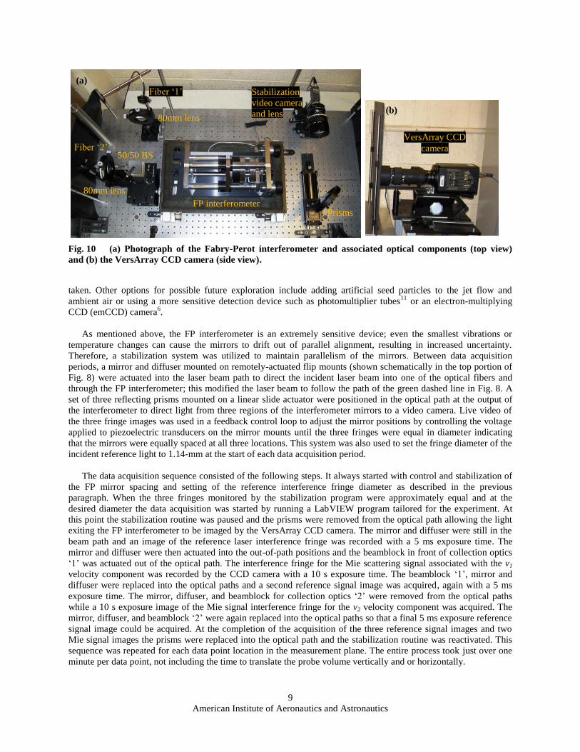
The 20-m long, 0.55-mm diameter multimode optical fibers transmitted the collected signals to the control room

where the FP interferometer and CCD camera that were used for spectral analysis of the light were located. The

interferometer must be isolated from the noisy jet because it is very sensitive to noise and vibrations. This portion of

the experiment is shown schematically in the bottom of Fig. 8 (labeled “CONTROL ROOM”) and a photograph of

the setup is shown in Fig. 10. The light exiting each fiber was collimated by an 80-mm focal length f/1.6 lens. The

two beams were combined with a 50/50 beam splitter so that light from both collection angles could be analyzed

using the same FP interferometer. As noted above, light from only one collection angle was analyzed at a time to

avoid ambiguity between the two sets of interference fringes. The combined beam paths were directed through the

FP interferometer which consisted of two planar 70-mm diameter air-spaced plates with 80% reflectivity coatings

and spacing of about 17.3-mm. The plate spacing and reflectivity prescribed a free spectral range of 8.7 GHz and

reflective finesse of approximately 15 for the instrument. The light exiting the FP interferometer was focused by a

Nikon 300-mm focal length lens at the detector of a Princeton Instruments VersArray back-illuminated, scientific-

grade CCD camera. The 512×512 imaging array had a 100% fill factor, 24×24-m pixels, 16-bit dynamic range,

high quantum efficiency, thermoelectric cooling, and low-noise electronics. The image of the optical fiber face was

approximately 2.1-mm (86 pixels) in diameter on the CCD detector. The reference signal images were acquired with

a 5 ms exposure time. Mie scattering data images were acquired with a 10 s exposure time to achieve scattering from

enough particles to have signal-to-noise of at least 2; the size distribution and number density of the particles in this

experiment were not known. Although 10 seconds was a somewhat long exposure time, this time could have been

greatly reduced by operating at locations and conditions where water condensation was naturally present in the flow;

there was no significant amount of water condensation at the x/D=1.9 location where the current measurements were

Fig. 9 Photograph of the small jet rig and the Doppler velocimetry measurement system.

Laser and propagation

optics (on back side of

mounting plates)

Collection

Optics „1‟

Cooling fan

x

y

z

Collection

Optics „2‟

Diffuser

Mirror

Beamblocks

Translation

mechanisms


9

taken. Other options for possible future exploration include adding artificial seed particles to the jet flow and

ambient air or using a more sensitive detection device such as photomultiplier tubes11

or an electron-multiplying

CCD (emCCD) camera6.

As mentioned above, the FP interferometer is an extremely sensitive device; even the smallest vibrations or

temperature changes can cause the mirrors to drift out of parallel alignment, resulting in increased uncertainty.

Therefore, a stabilization system was utilized to maintain parallelism of the mirrors. Between data acquisition

periods, a mirror and diffuser mounted on remotely-actuated flip mounts (shown schematically in the top portion of

Fig. 8) were actuated into the laser beam path to direct the incident laser beam into one of the optical fibers and

through the FP interferometer; this modified the laser beam to follow the path of the green dashed line in Fig. 8. A

set of three reflecting prisms mounted on a linear slide actuator were positioned in the optical path at the output of

the interferometer to direct light from three regions of the interferometer mirrors to a video camera. Live video of

the three fringe images was used in a feedback control loop to adjust the mirror positions by controlling the voltage

applied to piezoelectric transducers on the mirror mounts until the three fringes were equal in diameter indicating

that the mirrors were equally spaced at all three locations. This system was also used to set the fringe diameter of the

incident reference light to 1.14-mm at the start of each data acquisition period.

The data acquisition sequence consisted of the following steps. It always started with control and stabilization of

the FP mirror spacing and setting of the reference interference fringe diameter as described in the previous

paragraph. When the three fringes monitored by the stabilization program were approximately equal and at the

desired diameter the data acquisition was started by running a LabVIEW program tailored for the experiment. At

this point the stabilization routine was paused and the prisms were removed from the optical path allowing the light

exiting the FP interferometer to be imaged by the VersArray CCD camera. The mirror and diffuser were still in the

beam path and an image of the reference laser interference fringe was recorded with a 5 ms exposure time. The

mirror and diffuser were then actuated into the out-of-path positions and the beamblock in front of collection optics

„1‟ was actuated out of the optical path. The interference fringe for the Mie scattering signal associated with the v1

velocity component was recorded by the CCD camera with a 10 s exposure time. The beamblock „1‟, mirror and

diffuser were replaced into the optical paths and a second reference signal image was acquired, again with a 5 ms

exposure time. The mirror, diffuser, and beamblock for collection optics „2‟ were removed from the optical paths

while a 10 s exposure image of the Mie signal interference fringe for the v2 velocity component was acquired. The

mirror, diffuser, and beamblock „2‟ were again replaced into the optical paths so that a final 5 ms exposure reference

signal image could be acquired. At the completion of the acquisition of the three reference signal images and two

Mie signal images the prisms were replaced into the optical path and the stabilization routine was reactivated. This

sequence was repeated for each data point location in the measurement plane. The entire process took just over one

minute per data point, not including the time to translate the probe volume vertically and or horizontally.

Fig. 10 (a) Photograph of the Fabry-Perot interferometer and associated optical components (top view)

and (b) the VersArray CCD camera (side view).

(b)

VersArray CCD

camera

(a)

FP interferometer

Fiber „1‟

Fiber „2‟

80mm lens

80mm lens

50/50 BS

Stabilization

video camera

and lens

Prisms


10

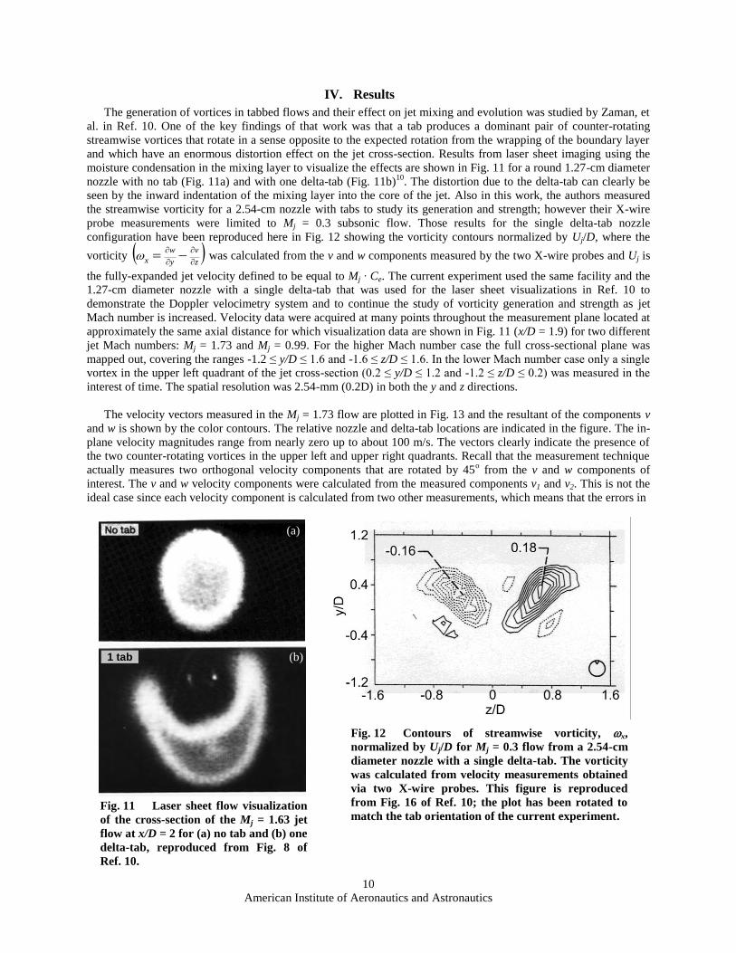
IV. Results

The generation of vortices in tabbed flows and their effect on jet mixing and evolution was studied by Zaman, et

al. in Ref. 10. One of the key findings of that work was that a tab produces a dominant pair of counter-rotating

streamwise vortices that rotate in a sense opposite to the expected rotation from the wrapping of the boundary layer

and which have an enormous distortion effect on the jet cross-section. Results from laser sheet imaging using the

moisture condensation in the mixing layer to visualize the effects are shown in Fig. 11 for a round 1.27-cm diameter

nozzle with no tab (Fig. 11a) and with one delta-tab (Fig. 11b)10

. The distortion due to the delta-tab can clearly be

seen by the inward indentation of the mixing layer into the core of the jet. Also in this work, the authors measured

the streamwise vorticity for a 2.54-cm nozzle with tabs to study its generation and strength; however their X-wire

probe measurements were limited to Mj = 0.3 subsonic flow. Those results for the single delta-tab nozzle

configuration have been reproduced here in Fig. 12 showing the vorticity contours normalized by Uj/D, where the

vorticity z

v

y

w

x

was calculated from the v and w components measured by the two X-wire probes and Uj is

the fully-expanded jet velocity defined to be equal to Mj ∙ Ce. The current experiment used the same facility and the

1.27-cm diameter nozzle with a single delta-tab that was used for the laser sheet visualizations in Ref. 10 to

demonstrate the Doppler velocimetry system and to continue the study of vorticity generation and strength as jet

Mach number is increased. Velocity data were acquired at many points throughout the measurement plane located at

approximately the same axial distance for which visualization data are shown in Fig. 11 (x/D = 1.9) for two different

jet Mach numbers: Mj = 1.73 and Mj = 0.99. For the higher Mach number case the full cross-sectional plane was

mapped out, covering the ranges -1.2 ≤ y/D ≤ 1.6 and -1.6 ≤ z/D ≤ 1.6. In the lower Mach number case only a single

vortex in the upper left quadrant of the jet cross-section (0.2 ≤ y/D ≤ 1.2 and -1.2 ≤ z/D ≤ 0.2) was measured in the

interest of time. The spatial resolution was 2.54-mm (0.2D) in both the y and z directions.

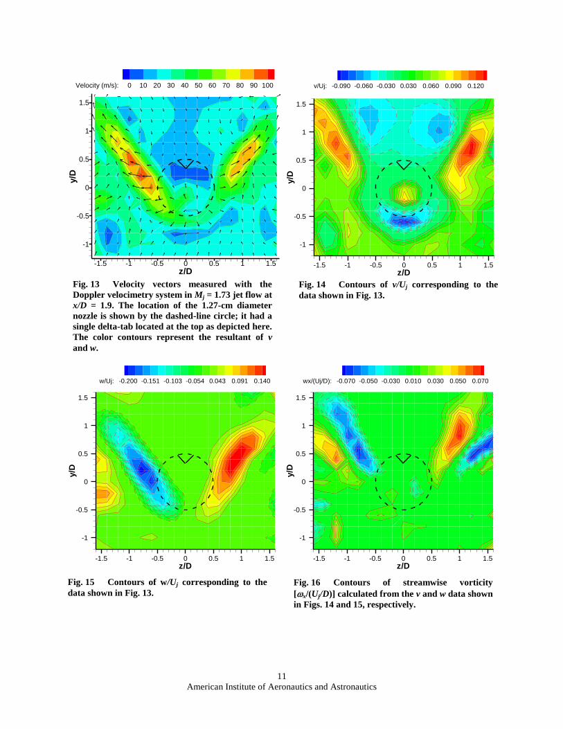
The velocity vectors measured in the Mj = 1.73 flow are plotted in Fig. 13 and the resultant of the components v

and w is shown by the color contours. The relative nozzle and delta-tab locations are indicated in the figure. The in-

plane velocity magnitudes range from nearly zero up to about 100 m/s. The vectors clearly indicate the presence of

the two counter-rotating vortices in the upper left and upper right quadrants. Recall that the measurement technique

actually measures two orthogonal velocity components that are rotated by 45o from the v and w components of

interest. The v and w velocity components were calculated from the measured components v1 and v2. This is not the

ideal case since each velocity component is calculated from two other measurements, which means that the errors in

Fig. 11 Laser sheet flow visualization

of the cross-section of the Mj = 1.63 jet

flow at x/D = 2 for (a) no tab and (b) one

delta-tab, reproduced from Fig. 8 of

Ref. 10.

Fig. 12 Contours of streamwise vorticity, x,

normalized by Uj/D for Mj = 0.3 flow from a 2.54-cm

diameter nozzle with a single delta-tab. The vorticity

was calculated from velocity measurements obtained

via two X-wire probes. This figure is reproduced

from Fig. 16 of Ref. 10; the plot has been rotated to

match the tab orientation of the current experiment.

(a)

_1 tab_ (b)


11

z/D

y/D

-1.5 -1 -0.5 0 0.5 1 1.5

-1

-0.5

0

0.5

1

1.5

Velocity (m/s): 0 10 20 30 40 50 60 70 80 90 100

z/D

y/D

-1.5 -1 -0.5 0 0.5 1 1.5

-1

-0.5

0

0.5

1

1.5

v/Uj: -0.090 -0.060 -0.030 0.030 0.060 0.090 0.120

z/D

y/D

-1.5 -1 -0.5 0 0.5 1 1.5

-1

-0.5

0

0.5

1

1.5

w/Uj: -0.200 -0.151 -0.103 -0.054 0.043 0.091 0.140

z/D

y/D

-1.5 -1 -0.5 0 0.5 1 1.5

-1

-0.5

0

0.5

1

1.5

wx/(Uj/D): -0.070 -0.050 -0.030 0.010 0.030 0.050 0.070

Fig. 13 Velocity vectors measured with the

Doppler velocimetry system in Mj = 1.73 jet flow at

x/D = 1.9. The location of the 1.27-cm diameter

nozzle is shown by the dashed-line circle; it had a

single delta-tab located at the top as depicted here.

The color contours represent the resultant of v

and w.

Fig. 14 Contours of v/Uj corresponding to the

data shown in Fig. 13.

Fig. 15 Contours of w/Uj corresponding to the


Fig. 16 Contours of streamwise vorticity

[x/(Uj/D)] calculated from the v and w data shown

in Figs. 14 and 15, respectively.


12

each measurement are compounded in the final velocity results; however in the interest of keeping the measurement

grid simple and the number of measurement locations to a minimum a rotation of coordinate axes was avoided. The

largest source of error in the velocity measurements was due to laser frequency drift (±17 MHz) during the data

acquisition. The standard deviation of the velocity error related to the change in reference fringe radius between two

consecutive reference images was about ±6 m/s. Since the v and w components were determined from a combination

of the two measured velocity components the errors add in quadrature giving a total error of about 8.5 m/s. To

alleviate some of this error the average radius between the two reference images acquired immediately before and

after the Mie image was used to determine the velocity measurement. The specifications for this frequency-

stabilized laser indicate that it should not exhibit the level of drift and instability that was experienced. The stability

of the laser will be investigated and improved, if possible, for future testing. The v and w velocities were normalized

by Uj and are plotted in Figs. 14 and 15, respectively. The velocities presented in Figs. 13-15 have all been

smoothed using a spatial filtering procedure that was also used for obtaining the gradients of v and w for the

calculation of vorticity. The filtering involved fitting a third-order polynomial through five adjacent data points and

updating the value of the data at the center. This spatial filtering took out some of the random scatter from the

velocity distribution and altered the magnitudes only slightly. The calculated streamwise vorticity was normalized

by Uj/D; where Uj for the supersonic jet was defined the same way as discussed in connection with Fig. 12. The

resulting vorticity contours are shown in Fig. 16 for the Mj = 1.73 flow. Even though the peak vorticity is

approximately 2.4 times lower than the peak vorticity in the Mj = 0.3 case shown in Fig. 12, it is clear that the

distributions are quite similar in the two cases.

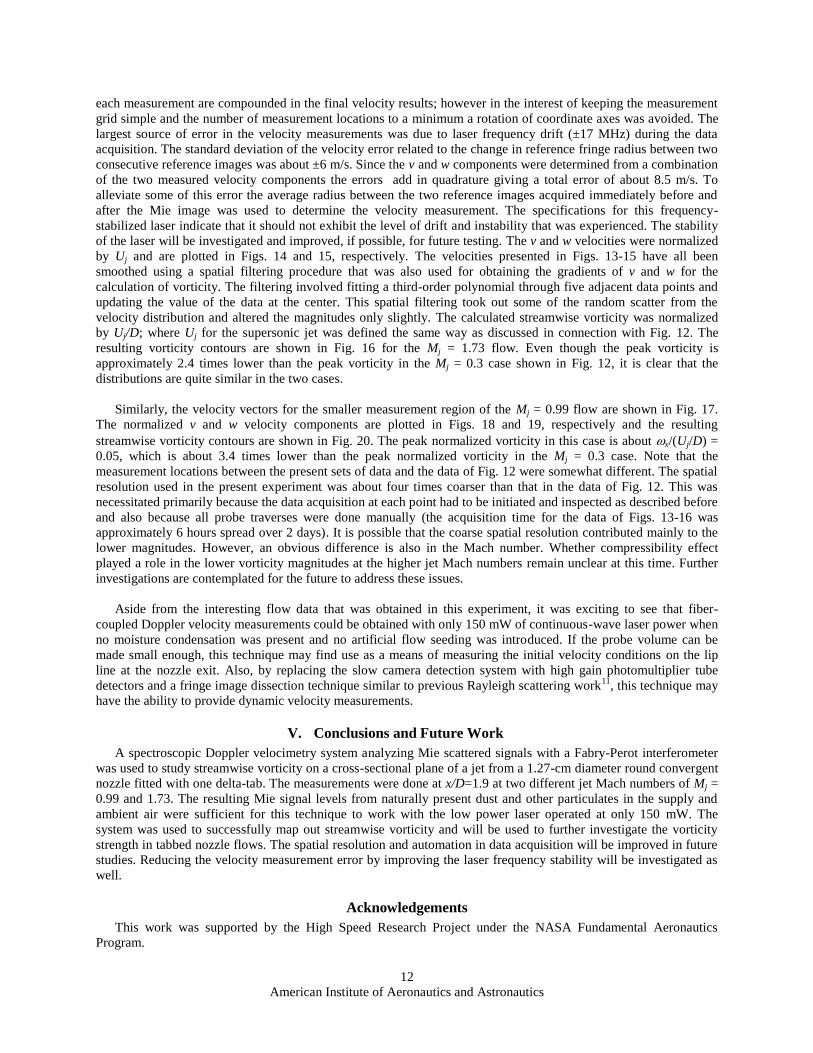
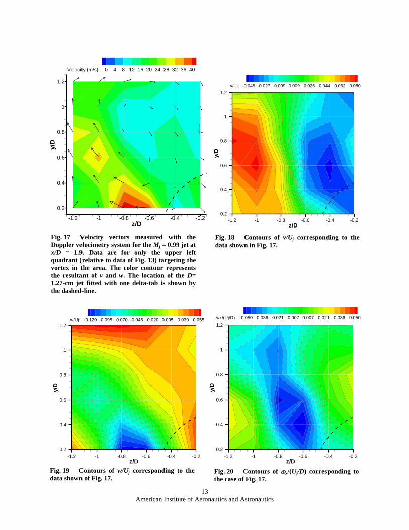
Similarly, the velocity vectors for the smaller measurement region of the Mj = 0.99 flow are shown in Fig. 17.

The normalized v and w velocity components are plotted in Figs. 18 and 19, respectively and the resulting

streamwise vorticity contours are shown in Fig. 20. The peak normalized vorticity in this case is about x/(Uj/D) =

0.05, which is about 3.4 times lower than the peak normalized vorticity in the Mj = 0.3 case. Note that the

measurement locations between the present sets of data and the data of Fig. 12 were somewhat different. The spatial

resolution used in the present experiment was about four times coarser than that in the data of Fig. 12. This was

necessitated primarily because the data acquisition at each point had to be initiated and inspected as described before

and also because all probe traverses were done manually (the acquisition time for the data of Figs. 13-16 was

approximately 6 hours spread over 2 days). It is possible that the coarse spatial resolution contributed mainly to the

lower magnitudes. However, an obvious difference is also in the Mach number. Whether compressibility effect

played a role in the lower vorticity magnitudes at the higher jet Mach numbers remain unclear at this time. Further

investigations are contemplated for the future to address these issues.

Aside from the interesting flow data that was obtained in this experiment, it was exciting to see that fiber-

coupled Doppler velocity measurements could be obtained with only 150 mW of continuous-wave laser power when

no moisture condensation was present and no artificial flow seeding was introduced. If the probe volume can be

made small enough, this technique may find use as a means of measuring the initial velocity conditions on the lip

line at the nozzle exit. Also, by replacing the slow camera detection system with high gain photomultiplier tube

detectors and a fringe image dissection technique similar to previous Rayleigh scattering work11

, this technique may

have the ability to provide dynamic velocity measurements.

V. Conclusions and Future Work

A spectroscopic Doppler velocimetry system analyzing Mie scattered signals with a Fabry-Perot interferometer

was used to study streamwise vorticity on a cross-sectional plane of a jet from a 1.27-cm diameter round convergent

nozzle fitted with one delta-tab. The measurements were done at x/D=1.9 at two different jet Mach numbers of Mj =

0.99 and 1.73. The resulting Mie signal levels from naturally present dust and other particulates in the supply and

ambient air were sufficient for this technique to work with the low power laser operated at only 150 mW. The

system was used to successfully map out streamwise vorticity and will be used to further investigate the vorticity

strength in tabbed nozzle flows. The spatial resolution and automation in data acquisition will be improved in future

studies. Reducing the velocity measurement error by improving the laser frequency stability will be investigated as

well.

Acknowledgements

This work was supported by the High Speed Research Project under the NASA Fundamental Aeronautics

Program.


13

z/D

y/D

-1.2 -1 -0.8 -0.6 -0.4 -0.2

0.2

0.4

0.6

0.8

1

1.2

Velocity (m/s): 0 4 8 12 16 20 24 28 32 36 40

z/D

y/D

-1.2 -1 -0.8 -0.6 -0.4 -0.2

0.2

0.4

0.6

0.8

1

1.2

v/Uj: -0.045 -0.027 -0.009 0.009 0.026 0.044 0.062 0.080

z/D

y/D

-1.2 -1 -0.8 -0.6 -0.4 -0.2

0.2

0.4

0.6

0.8

1

1.2

w/Uj: -0.120 -0.095 -0.070 -0.045 -0.020 0.005 0.030 0.055

z/D

y/D

-1.2 -1 -0.8 -0.6 -0.4 -0.2

0.2

0.4

0.6

0.8

1

1.2

wx/(Uj/D): -0.050 -0.036 -0.021 -0.007 0.007 0.021 0.036 0.050

Fig. 17 Velocity vectors measured with the

Doppler velocimetry system for the Mj = 0.99 jet at

x/D = 1.9. Data are for only the upper left

quadrant (relative to data of Fig. 13) targeting the

vortex in the area. The color contour represents

the resultant of v and w. The location of the D=

1.27-cm jet fitted with one delta-tab is shown by

the dashed-line.

Fig. 18 Contours of v/Uj corresponding to the


Fig. 19 Contours of w/Uj corresponding to the

data shown of Fig. 17. Fig. 20 Contours of x/(Uj/D) corresponding to

the case of Fig. 17.


14

References 1Raffel, M., Willert, C., and Kompenhans, J., Particle Image Velocimetry, Springer, New York, 1998. 2Tropea, C., “Laser Doppler Anemometry: Recent Developments and Future Challenges,” Meas. Sci. Technol., Vol. 6, No. 6,

1995, pp. 605-619. 3McKenzie, R. L., “Measurement Capabilities of Planar Doppler Velocimetry Using Pulsed Lasers,” Applied Optics, Vol. 35

No. 6, 1996, pp. 948-964.

4Miles, R. B., Lempert, W. R., and Forkey, J. N., “Laser Rayleigh Scattering,” Meas. Sci. Technol., Vol. 12, No. 5, 2001, pp.

R33-R51. 5Mielke, A. F., Elam, K. A., and Sung, C. J., “Multiproperty Measurements at High Sampling Rates Using Rayleigh

Scattering,” AIAA Journal, Vol. 47, No. 4, 2009, pp. 850-862. 6Bivolaru, D., Cutler, A. D., Danehy, P. M., Gaffney, R. L., and Baurle, R. A., “Spatially and Temporally Resolved

Measurements of Velocity in a H2-air Combustion-heated Supersonic Jet,” AIAA-2009-27, 2009. 7Vaughan, J. M., The Fabry Perot Interferometer, History, Theory, Practice, and Applications, Adam Hilger, Philadelphia,

1989, pp. 89-134. 8Bohren, C. F., Huffman, D. R., Absorption and Scattering of Light by Small Particles, John Wiley & Sons, New York, 1983,

pp. 82-104, 447. 9Edwards, R. V., Processing Random Data: Statistics for Engineers and Scientists, World Scientific, New Jersey, 2006,

pp.91-97. 10Zaman, K. B. M. Q., Reeder, M. F., and Samimy, M., “Control of an axisymmetric jet using vortex generators,” Phys.

Fluids, Vol. 6, No. 2, 1994, pp. 778-793. 11Panda, J., Seasholtz, R. G., and Elam, K. A., “Investigation of noise sources in high-speed jets via correlation

measurements,” Journal of Fluid Mechanics, Vol. 537, 2005, pp. 349-385.