Download - Application of a Dynamic Pressure-Sinkage Relationship for ...

Int. J. Vehicle Autonomous Systems, Vol. x, No. x, xxxx 1

Application of a Dynamic Pressure-SinkageRelationship for Lightweight Mobile Robots

Rishad A. Irani*Dalhousie University,Department of Mechanical EngineeringHalifax, Nova Scotia B3J 1Z1, CanadaE-mail: [email protected]*Corresponding author

Robert J. BauerDalhousie University,Department of Mechanical EngineeringHalifax, Nova Scotia B3J 1Z1, CanadaE-mail: [email protected]

AndrewWarkentinDalhousie University,Department of Mechanical EngineeringHalifax, Nova Scotia B3J 1Z1, CanadaE-mail: [email protected]

Abstract: This paper investigates a dynamic pressure-sinkagerelationship which can be used in a wheel-soil model to better captureperiodic variations observed in sinkage, drawbar pull and normal forceas a rigid wheel interacts with loose sandy soil. The dynamic wheel-soilmodel can be used for wheels with or without grousers. Several casestudies are presented to demonstrate the usefulness and applicability ofthis dynamic pressure-sinkage relationship. Hill climbing experimentswere carried out using a smooth-wheel micro rover with a fixedsuspension to confirm operational regions of the dynamic pressure-sinkage relationship. Single wheel testbed experiments were carried outto determine how well the model can predict changes in the numberand length of the grousers on the wheel. It was concluded that dynamicpressure-sinkage relationship can predict the observed oscillations inthe sinkage, drawbar pull and normal force with a single tuning caseas the slip ratio and the configuration of the wheel changes.

Keywords: Terramechanics; Sandy Soil Modeling; Pressure-SinkageRelationship; Rigid Wheel; Grousers

Biographical notes: Rishad Irani completed his BASc at theUniversity of Windsor in 2003 and his MASc at Dalhousie Universityin 2006. Rishad completed his PhD in 2011 by examining the mobilityissues that face the next generation of Mars Rovers under thesupervision of Dr. Robert Bauer. Robert J. Bauer received a BASc in

Copyright c⃝ 2011 Inderscience Enterprises Ltd.

2 R.A. Irani, R.J. Bauer and A. Warkentin

Mechanical Engineering from the University of Waterloo in 1994. In

1998, he received a PhD in Aerospace Engineering from the University

of Toronto. In 1998, he joined the Mechanical Engineering faculty

at Dalhousie University and is currently a Professor carrying out

research in process modeling and control of dynamic systems. Andrew

Warkentin completed his Bachelor’s degree in 1991 and Master’s degree

in 1993 at McMaster University and went on to complete a PhD

at the University of Waterloo in 1997. He continued his research at

Waterloo with an NSERC Post-Doctoral Fellowship. In 1998, he joined

Dalhousie University where he teaches Design and Manufacturing in

the Department of Mechanical Engineering.

In the past few years there has been a considerable amount of researchinvolving lightweight mobile robots — specifically, planetary rovers. Much ofthis work stems from several planetary exploratory missions by various agenciesincluding National Aeronautics and Space Administration (NASA), the EuropeanSpace Agency (ESA) and Japan Aerospace Exploration Agency (JAXA). Therehas even been mobilization in the private sector for planetary rovers and severalofficial teams which are privately funded and competing in the Google Lunar XPRIZE competition.

To enhance the mobility of any of these lightweight planetary rovers orexploratory vehicles a high fidelity wheel-soil interaction model is needed.Typically, empirically-based static or quasi-static models are used for these low-speed applications. Lyasko (2010) reported that the most common formulation forthe wheel-soil interaction with rigid wheels is based on the work of Bekker (1969),which is a semi-empirical quasi-static model. Despite the significant research todevelop wheel-soil interaction models, Azimi et al. (2010) concluded that thereis still a need for further validation and improvement of the traditional semi-empirical quasi-static terramechanic model of Bekker (1969) and Wong (2010).Irani et al. (2010a) introduced a dynamic wheel-soil interaction model whichadvances classic work by Bekker and Wong, such that the oscillations about thepredicted or modeled drawbar pull can now be represented for a smooth rigidwheel. Irani et al. (2011a) used Reece’s (1965) pressure-sinkage relationship toadvance their own model and presented a terramechanic model which focuseson predicting the oscillations in the drawbar pull, normal force and sinkage forlightweight vehicles for a wheel with grousers.

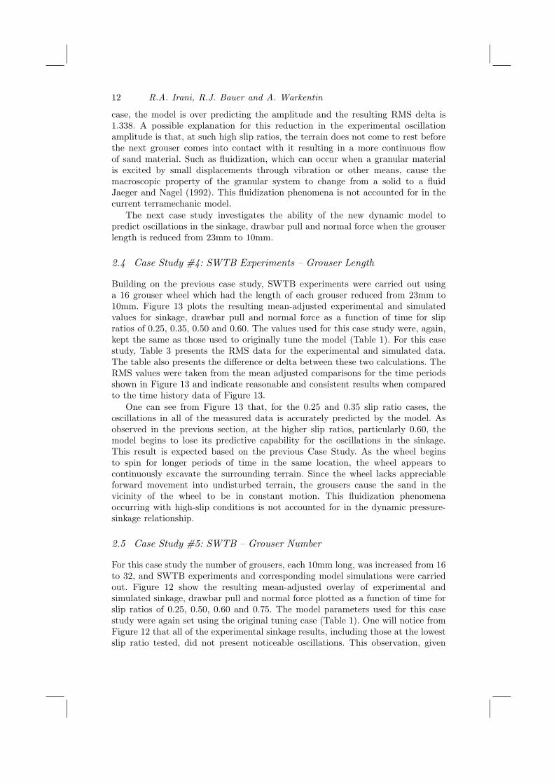
This paper presents a series of case studies using the more advanced semi-empirical dynamic terramechanic model which was developed by Irani et al.(2011a). The work presented here will feature case studies to show how the modelcan be used to accurately predict the fluctuations in the measured data of thewheel-soil interaction for a rigid wheel operating in sandy soil with and withoutgrousers. Figure 1 shows a sample of these oscillations observed in the measureddata from a single-wheel testbed for a 200mm diameter rigid wheel with 16, 23mmlong grousers operating at a slip ratio of 0.50. It will also be shown that the modelis able to predict these fluctuations as the slip ratio and the configuration of thegrouser wheel changes with no re-calibration of the model.

Application of a Dynamic Pressure-Sinkage Relationship 3

1 Terramechanic Model

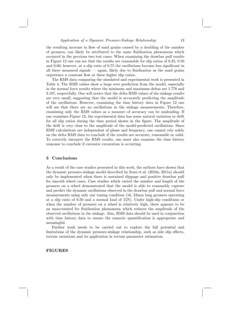
Figure 2 shows the forces and stresses which need to be calculated so that they canbe used to determine the trafficability, motion planning and/or control algorithmsfor the full vehicle. The classic terramechanic model for a smooth rigid wheeldescribed by Bekker (1969) assumes that the pressure p under a wheel can beapproximated by a flat plate with an exponential function as follows:

p (z) =

(kcb

+ kϕ

)zn (1)

where z is the instantaneous sinkage, n is the sinkage exponent, b is the smallerdimension of the wheels contact patch and kc and kϕ are an empirical coefficientswhich are found though infield bevameter testing (Bekker (1969)). Reece (1965)proposed that the pressure-sinkage relationship can also be expressed as a functionof two dimensionless coefficients k′c and k′ϕ, the wheel sinkage z and wheel widthb, such that:

p (z) =(ck′c + γbk′ϕ

) (zb

)n

(2)

Here, c and γ are the terrain’s cohesion and weight density respectively and k′cand k′ϕ can be tuned to the specific terrain and operating conditions. The dynamicmodel proposed by Irani et al. (2011a) uses the Reece pressure-sinkage relationshipto estimate the oscillations seen in the sinkage, drawbar pull and normal load. Thedynamic pressure-sinkage relationship has the general form:

p(z) =(ck′c + γbk′ϕ

) (zb

)n

+A sin (ωt+Φ) (3)

where t is time and Φ is an optional phase shift that can be applied to the modelfor fitting the simulation predictions to experimental data or applying a correctionto account for the initial orientation of the grousers. The A term is the amplitudeof the oscillations and ω is the frequency at which they occur. The traditionalterramechanic model will estimate the average normal stress by a curve governedby Equation (1) which does not explicitly account for the wheel geometry in theclassic terramechanic model. Karafiath and Nowatzki (1978) proposed that thenormal stress distribution is not a smooth curve but rather is a discontinuousfunction as the grousers will affect the stresses acting on the terrain. Irani et al.(2011a) has shown that the dynamic model is able to estimate the fluctuationsand variations in the pressure-sinkage relationship that is caused by the presenceof grousers which Karafiath and Nowatzki hypothesized.

The modified Mohr Coulomb failure criteria developed by Janosi andHanamoto (1961) can be used to determine the shear stress τ acting along thewheel-soil interface such that:

τ (θ) = (c+ σ (θ) tanϕ)[1− e−j(θ)/K

](4)


where θ angular location of the wheel-soil interface, ϕ is the internal angle offriction, K is a soil property known as the shear deformation modulus, and j hasthe form:

j (θ) = r [θf − θ − (1− i) (sin θf − sin θ)] (5)

The slip ratio i for this work is defined as:

i =ωwr − Vx

ωwr(6)

where ωw is the angular velocity of the wheel, r is the radius of the wheel, and Vx

is the translational velocity of the wheel centre.Converting p(z) to polar coordinates, the pressure becomes the normal stress

σ(θ) as shown in Figure 2 and shear stress τ(θ) can be calculated by Equation(4) in the wheel-soil interaction. The vertical force Fz is calculated by taking thearea integrals of the stresses in the vertical direction and the drawbar pull DPis computed by the area integrals of the stresses in the horizontal direction, suchthat:

Fz = rb

∫ θf

θr

(τ (θ) sin θ + σ (θ) cos θ) dθ (7)

DP = Fx = rb

∫ θf

θr

(τ (θ) cos θ − σ (θ) sin θ) dθ (8)

The entry and departure angles, θf and θr, of the wheel-soil interface arecalculated by:

θf = cos−1 (1− z/r) (9)

θr = − cos−1 (1− ηz/r) (10)

where η, also shown in Figure 2, is a dimensionless empirical parameter whichcompares the nominal wheel sinkage z to the depth of the track left by the wheel.Ishigami et al. (2007) states that η is related to the soil properties, slip ratio andthe wheel surface pattern.

If one uses the Reece pressure sinkage relationship shown in Equation (2), thenthe resulting calculated drawbar pull, normal force and sinkage would not varyonce steady-state operation is reached. However, if one were to use the dynamicpressure-sinkage relationship shown in Equation (3) instead, then the drawbar pull,normal force and sinkage calculated by the analytical model would vary even aftersteady-state operation is reached, which more closely approximates data seen fromexperimental work Apostolopoulos et al. (2003); Arvidson et al. (2010); Irani et al.(2010a, 2011a) and shown in Figure 10. It should be pointed out that the dynamicmodel can be used for both smooth and grouser wheels operating in loose sandysoil. The following section examines the new parameters found in the dynamicpressure sinkage relationship.


1.1 Frequency ω

For a grouser wheel the frequency ω in Equation (3) is related to the spacing ofthe grouser blades and angular velocity of the wheel. Therefore, ω for a grouserwheel becomes:

ω =ωw

ng(11)

where ng is the number of grousers and ωw is the angular velocity of the wheel inradians per second.

When a smooth wheel (no grousers) operates in sandy soil oscillations inthe measured data are still observed. It is believed that the change in the localdensity around the wheel-soil interface is causing the oscillations in the data andrepeatable ridges in the sand. Through empirical testing it was found that thefrequency of the oscillations was linearly related to the slip ratio and independentof the normal load. As a result, the following empirical equation can be used toestimate the frequency as a function of the slip ratio i:

ω = −36.9i+ 36.5 (12)

This equation was developed for a smooth rigid wheel of diameter .02 [m] andwidth 0.075[m] operating in sandy soil using a normal load of 14.9N (Irani et al.(2010a)), and a normal load of 47.7N was successfully used as a test case. A firstorder least-squares fit was performed for the 14.9N normal load data resulting inan R2 value of 0.94. Equation (12) is unique unique to the test case for which itwas developed. Therefore, with different terrains and/or wheel dimensions a newempirical equation must be found.

1.2 Amplitude A

There are two main factors that can contribute to the amplitude term A ofEquation (3): a change in the local density near the wheel-soil interface and theadded stress which grousers add to the interface. Thus, the amplitude term A canbe written as:

A = Aσ +Aγ (13)

where Aσ is related to the passive stresses which the terrain experiences due theadded traction which grousers apply (for a smooth wheel Aσ would be zero) andAγ is related to the local soil density change around the wheel caused by the soildeformation which occurs as the wheel travels through the terrain. The followingsections will further explain and examine these two amplitude terms.

1.2.1 Passive Stresses; Aσ

Wong (2010) demonstrates how a grouser blade creates passive stresses to increasethe tractive effort of a vehicle. The amplitude of the oscillations of the pressure-sinkage relationship could be a function of the passive stresses which are computedby Wong (2010):

σp = γzNϕ + qNϕ + 2c√Nϕ (14)


where the flow value Nϕ is given by:

Nϕ = tan2(45◦ +

ϕ

2

)(15)

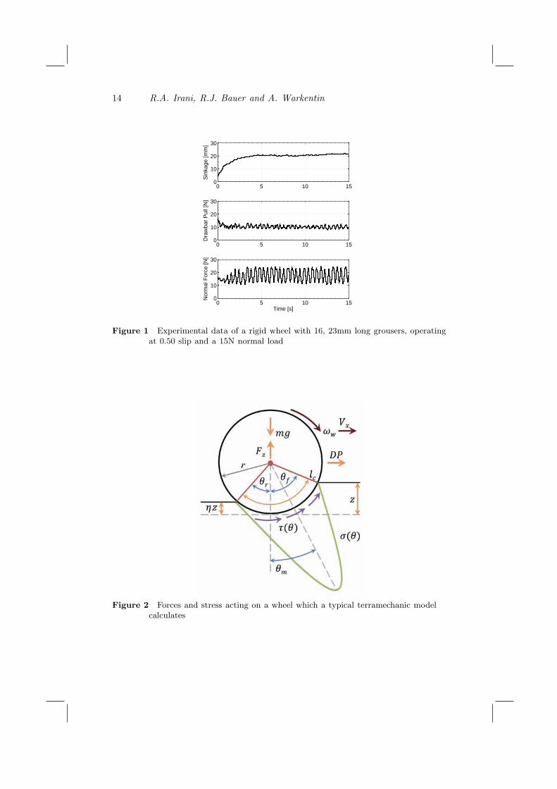
In Equation (14), q is referred to as surcharge and is the additional pressureapplied to the surface of the terrain from external sources. In a wheel-soilinteraction, where the grouser of length hb is exerting a passive stress on the soil,the normal stress σ(θ) from the smooth wheel section just ahead of the grouserwould act as a surcharge. The length over which this surcharge contributes to thepassive stresses is calculated by Wong (2001):

lqp =hb

tan(45◦ − ϕ

2

) (16)

A passive stress acts in the same direction as the shear stress and, therefore,contributes additional components to the vertical and horizontal forces (seeEquations (8) and (7)). Figure 3 shows the passive stress zones on the grouser face.

The formulation of the passive stresses shown in Equation (14) assumes thesurcharge is uniform along the length lqp. However, regardless of which pressuresinkage relationship one uses, at every depth along the wheel-soil interface thereis a different stress state acting on the wheel because of the wheel’s curvature.Thus, the surcharge acting on the grouser will not be uniform during the wheel-soilinteraction. The mean pressure from the pressure-sinkage relationship acting alonglqp can be used to approximate the surcharge q. Also, when more than one grouseris in contact with the terrain, the mean of the passive stresses will be proportionalto the amplitude term Aσ. Thus,

Aσ = k′gσ̄p (17)

where k′g is an empirical dimensionless coefficient and σ̄p is the mean of the passivestresses acting on the grouser blades which are in contact with the wheel.

The second amplitude term Aγ in Equation (13) is described in the followingsection.

1.2.2 Change in Local Density; Aγ

As an object travels through loose sandy soil there will be some form ofdeformation around the object. The deformation around the object will cause thegranular particles to shift and fill in voids of the loosely pack structure of the initialterrain. This process can occur when a slipping wheel travels through loose sandysoil. If the local density increases around the wheel, then the strength of the sandwould increase and the normal and shear stress which the wheel can exert on thesoil (and, as a result, the vertical and horizontal forces acting on the wheel) willvary (Holtz et al. (1981)).

To account for this effect, amplitude term Aγ is related to the local change inthe weight density of the soil around the wheel and the contact length lc, which isthe characteristic length describing the interface, as follows:

Aγ = k′alcdγ (18)


where k′a is an empirical dimensionless coefficient and dγ is the change in sanddensity which was taken as 10% of the initial undisturbed terrain. To determinethe change in the density a soil sample was placed on a shaker table and excited at30Hz and images where recorded so that a time-lapse analysis could be preformed.It was observed in time-lapse analysis that there was a 6.5% change in the densitywithin 0.5 seconds and maximum of 14% change in density after 3 seconds. A valueof 10% was used to approximate the density change as the wheel passed throughthe specific sand in this research. It should be pointed out that not all terrainswill exhibit this drastic variation in the density. Before assigning a value of dγ ork′a one must first assess the degree to which the terrain experiences a change indensity from small displacements or excitation. This assessment can come fromlaboratory testing with a shaker table or through in-situ testing with a compactor.Terrains which do not experience large variations in their density will have low dγand possibly a negligible k′a. A k′a of zero can be assigned if a slipping smooth-wheel does not produce any ridges in the terrain or in the sinkage, drawbar pullor normal force measurements. The contact length lc is shown in Figure 2 and canbe calculated by the following:

lc = r (|θf |+ |θr|) (19)

where r is the radius of the wheel, and θf and θr are the corresponding entryand departure angles found from Equations (9) and (10), respectively. SubstitutingEquation (18), (17) and (13) into Equation (3) yields the final dynamic pressure-sinkage relationship for the terramechanic model:

p(z) =(ck′c + γbk′ϕ

) (zb

)n

+ (k′gσ̄p + k′alcdγ) sin (ωt+Φ) (20)

1.3 Implementation of the Dynamic Model

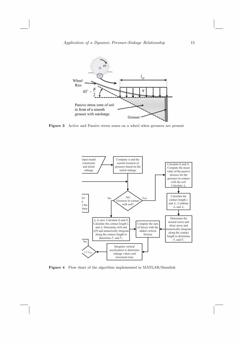
To implement the terramechanic model, an algorithm was constructed inMATLAB/Simulink as follows:

1. Model constants and constraints are inputted and an initial static sinkage isprescribed for t = to. The frequency ω is constant for the duration of testrun and, therefore, Equation (12) or (11) can be calculated at this step.

2. Determine if any grousers are in contact with the soil and calculate θf andθr. Compute the mean value of the passive stress σ̄p by first determiningthe surcharge q for each of the grousers in contact with the terrain in theirrespective locations so that Aσ can be computed.

3. Calculate Aγ from Equation (18) by first computing the contact length lcfrom θf and θr. A in Equation (13) can now be applied to combine Aσ andAγ .

4. Determine the normal stress σ(θ) and shear stress τ(θ) and numericallyintegrate along the contact length to determine Fz and Fx using Equations(7) and (8).


5. Frictional damping Ff needs to be applied to the vertical direction as theterramechanic model does not account for any soil damping. For this work,viscous friction was assumed using a friction coefficient of 800 Ns/m. Thesinkage acceleration can be determined from the sum of the forces in thevertical direction and then the sinkage acceleration can be integrated twicewith respect to time such that an updated sinkage value is determined andcan be used in the next time-step.

6. Return to Step 2 with the updated value of sinkage.

The algorithm presented above is shown in a flowchart found in Figure 4.

2 Case Studies

The following sections present a series of case studies to help demonstrate theusefulness and applicability of the dynamic pressure-sinkage relationship describedby Equation (20). The first case study examines how smooth wheels mounted ona 4-wheeled micro rover testbed interact with sandy soil at different slip ratios asthe rover navigates an incline. The second case study uses passive stress theory tosimulate a wheel grouser interacting with the soil. The third case study investigatesthe influence of grouser height on the wheel-soil interaction at different slip ratiosusing measurements from a single wheel testbed. The fourth case study also uses asingle wheel testbed and focuses on how wheels with different number of grousersinteract with sandy soil at different slip ratios.

2.1 Case Study #1: Smooth Wheel Rover Tests

The single-wheel testbed research performed by Apostolopoulos et al. (2003)used 15.2kg inflatable wheels with a radius of 70cm along the compressed axis,and a contact width of approximately 1m. Apostolopoulos et al. mentioned thatrepeatable ridges 5cm wide and 3cm tall were found in the wheel track as itoperated in sandy soil. Ishigami’s PhD thesis (2008) presented images showingsimilar repeating ridges in the track of a smooth rigid wheel operating in a Lunarsimulant or Toyoura Sand. Ishigamis work did not mention or focus on these ridgesin the wheel track. As previously mentioned, Irani et al. (2010a) has developeda dynamic pressure-sinkage model after noticing ridges in the track of a smoothwheel operating in sandy soil. However, all of the documented cases found in theliterature come from tests preformed on single-wheel testbeds and, therefore, thequestion must be answered: Are these ridges an artifact of the single-wheel testbedor are the ridges a natural phenomena that occurs with a real lightweight mobilerobot operating in sandy soil?

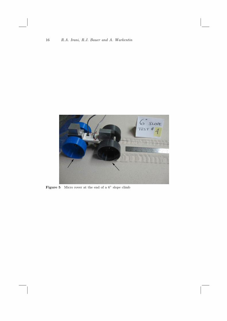
To answer this question a four-wheel micro rover having 100mm diametersmooth wheels was constructed and tested in sandy soil. The rear wheels weredriven through a 505.9:1 geartrain while the front wheels were free to rotate.Given the dynamic pressure-sinkage relationship presented in Section 1, it washypothesized that the rear wheels, when slipping, would produce repeatable ridges,and that the front wheel would leave a smooth track since their drawbar pull wouldbe negative. A tachometer was used to determine the angular velocity of the wheels


and a potentiometer was used to record the linear translation of the 1.6kg vehicle.The rear wheels rotated at an average speed of 9.5rpm with a standard deviationof 0.21.

To achieve a repeatable and consistent slipping condition, hill climbing testswere carried out at 3.5◦, 5◦ and 6◦ (maximum inclination which the rovercould climb) which corresponded to rear-wheel slip ratios of 0.8, 0.95 and 0.96,respectively. Incline angles between 0◦ and 3.5◦ did not produce consistent orrepeatable slip conditions. The reason for the irregular results at low inclines islikely from the initial conditions of the test sand where, before each test, thesand was manually mixed and leveled with a scraper tool. It is likely that thelocal density was not perfectly uniform after this manual preparation process and,therefore, when the micro rover traversed the terrain, any small variations in theterrain influenced the mobility of the vehicle. Once the slip ratio increased to 0.8,the micro rover’s rear wheels produced consistent and repeatable ridges in the sandas predicted.

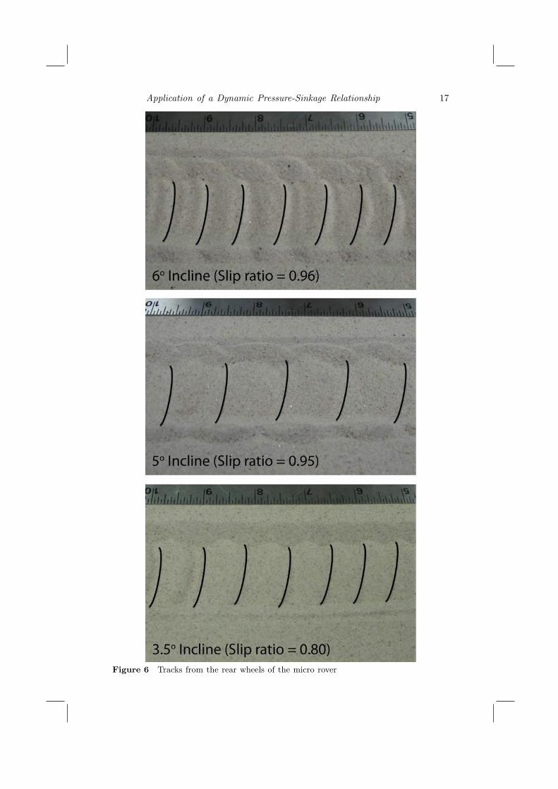
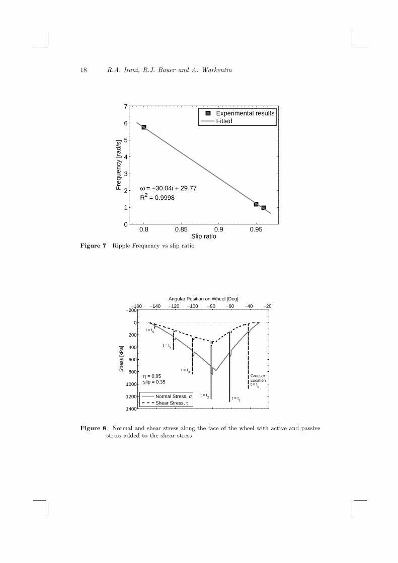
The results of these tests can be seen in Figure 5 which shows the micro roverand its tracks with the ridges at the various slip ratios. Also, as predicted andshown in Figure 5, the un-powered front wheel produced a smooth flat track.Figure 6 shows a selection of the tracks from the rear wheels for the inclines testedand, in this figure, heavy lines have been digitally superimposed to help the readeridentify the ridges. When a linear least squares curve fit was performed on thethree slip ratios tested, a linear relationship was found. This linear result fromthe micro rover case study confirms earlier published work of Irani et al. (2010a)where it was shown that there is linear relationship between the frequency of theoscillations and the slip ratio when a smooth wheel was tested on a single-wheeltestbed (SWTB).

The results of this case study also indicate that the dynamic pressure-sinkagemodel described by Equation (20) should only be used when positive drawbar pullis established at a sustained slipping state. The case study also shows that theridges in the sand are not an artifact of the single-wheel testbed — they are, infact, a natural phenomena that occurs when a lightweight mobile robot operates insandy soil. It is believed that the ridges are caused be the local change in densityon the wheel-soil interface (Irani et al. (2011a). Therefore, if a terrain does notexperience a density variation when a smooth slipping wheel passes though it, ak′a of zero can be assigned to that wheel-soil interaction.

The micro rover was tested with smooth wheels; however, most wheels havegrousers to aid their tractive effort.

2.2 Case Study #2: Passive Stress Theory – Dynamic Effect of Grousers

A theoretical case study was performed to examine how passive stresses from agrouser on a rotating wheel affect the resulting normal and shear stress acting onthe wheel. In this case study a wheel was simulated which:

• was 20 cm in diameter

• operated at a slip ratio of 0.35 with a sinkage of 5cm while η is 0.95

• had grousers that were 15mm long and 3mm thick


The results of this theoretical case study are shown in Figure 8 which plots thecorresponding normal and shear stress as a function of angular position along thewheel as the grousers travel through the terrain in sequential time steps. As shownin Figure 8, when t = to the grouser is located at −40◦ and then, at the next time-step, (t = t1) the grouser is located at −60◦. One will notice that, although thepassive stresses from a grouser have little effect on the normal stress, the passivestresses significantly affect the shear stress (up to an order of magnitude largerthan the nominal shear stress). The grouser thickness only contributes about 15%to the normal stress when compared to the overall magnitude of the normal stressand only acts over the width of the grouser. Furthermore, it can be seen that thepassive stress contribution of an individual grouser varies as it moves through theterrain, and variations in the resulting normal and shear stress distribution aroundthe wheel cause variations in the resulting forces acting on the wheel. As a resultof this case study it becomes clear that passive stresses should be incorporatedinto the pressure-sinkage relationship.

2.3 Case Study #3: SWTB Experiments – Dynamic Effect of Grousers

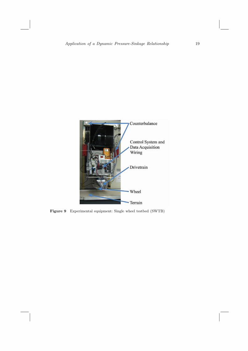
A series of experiments were carried out on a single-wheel testbed (SWTB) usinga wheel with grousers to study the ability of the dynamic pressure sinkage modeldescribed by Equation (20) (Irani et al. (2011a)) to predict the normal force,drawbar pull and sinkage for different slip ratios and grouser geometry. Figure 9shows the experimental setup of the SWTB used during testing.

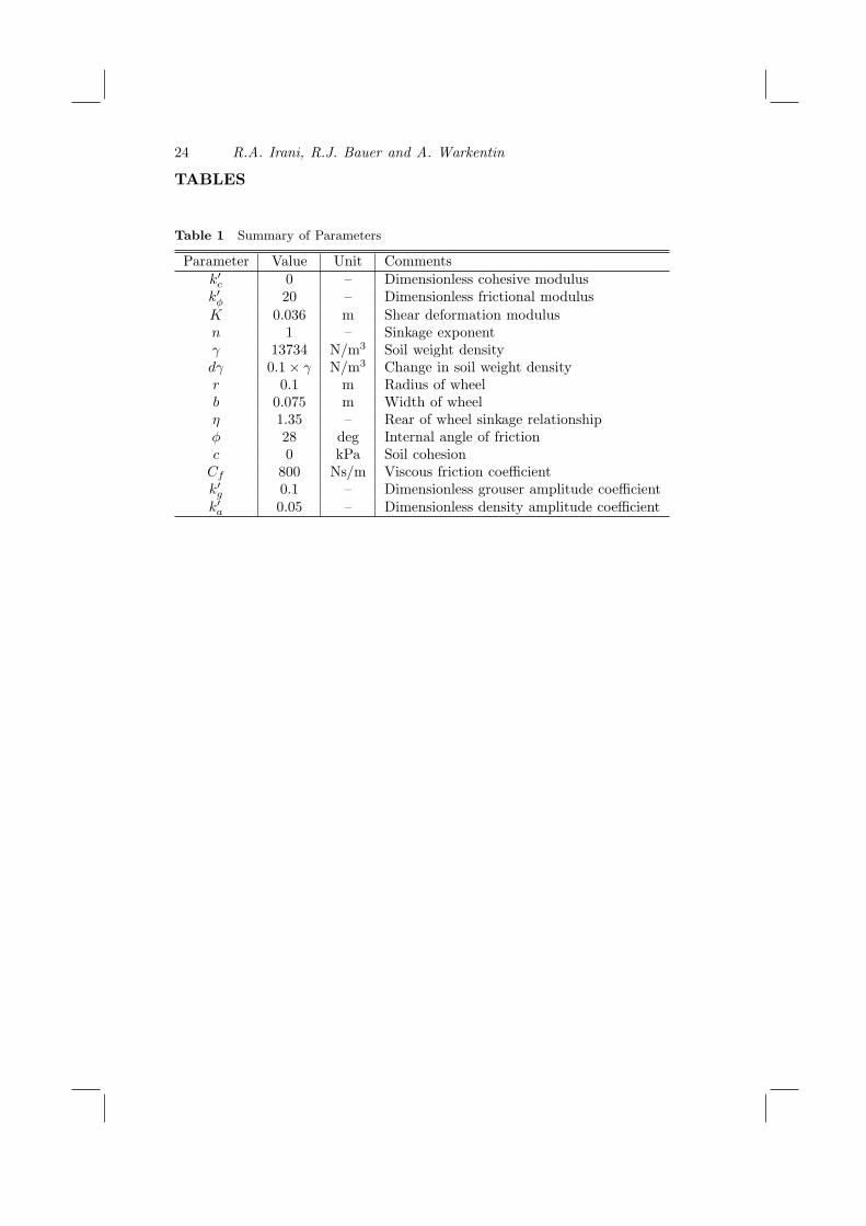
A wheel with 16, 23mm long grousers operating at a slip ratio of 0.50 anda normal load of 15N was used as the sole tuning case for the terramechanicmodel described in Section 1. The parameters used in the model and their valuescan be found in Table 1. The shear deformation modulus K and ϕ can be foundthrough triaxial, ring shear or shear box laboratory testing. Typically, in dry sandthe cohesion c is very low and can be found through a ring shear or shear boxlaboratory testing (Wong (2010) and Holtz et al. (1981)). In the case of the sandused in this research the cohesion was below the sensitivity of the equipment andtherefore it was taken as zero for this work. Taking sand as cohesionless is notuncommon in soil mechanics (Holtz et al. (1981)). The initial weight density of thesand was measured in the laboratory by measuring the weight of a known volumeof the sand. The sinkage exponent n is taken as 1 for dry sands (Wong (2010)).The non-dimensional coefficient k′c was set to zero as suggested by Wong (2001;2010). The value of η has said to be a function of the wheel’s geometry, soil ratioand the soil conditions (Ishigami et al. (2007)). If one has definite measurementsfor η in various scenarios, those values of η should be used. The rear of wheelsinkage relationship η was visually inspected to be 1.35 for the test case and usedfor all other cases as the predictive abilities of the model are examined in thiswork. Through experimental experience the value of 1.35 is not unreasonable fora variety of scenarios with the experimental wheels and sand used in this work.The only parameter left in the classic terramechanic model is the non-dimensionalcoefficient k′ϕ. This parameter was manually tuned to a value of 20. The tuningwas done by slowly increasing the value of k′ϕ until the means of the measureddata were reasonably represented by the simulation. Once the classic model wastuned, values for k′g and k′a of the new dynamic model need to be determined. For a


grouser wheel the contribution of the passive stresses would dominate the tractiveeffort and therefore, a ratio of 2:1 was used for k′g : k′a. To manually tune the modela value of k′g was set and k′a was calculated. The value of k′g was then slowlyincreased and the resulting amplitude of the oscillations were observed in thesimulated results until a reasonable approximation was found for the experimentalresults for the sole tuning case.

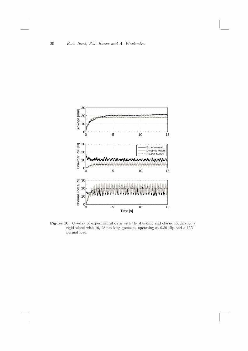
The parameters in Table 1 were held constant throughout all of thesimulations carried out for this case study and the next two case studies.Figure 10 plots the sinkage, drawbar pull and normal load as a functiontime and overlays experimental results with the dynamic pressure-sinkage modeldescribed by Equation (20) and Bekker’s traditional terramechanic model.Bekker’s terramechanic model was able to reasonably model the mean sinkageand normal force; however, it under predicted the drawbar pull by 5N for thiscase. This under prediction can be attributed to the fact that Bekker’s traditionalterramechanics model was originally developed for wheels larger than 50 cm(Bekker (1969); Wong (2001); Meirion-Griffith and Spenko (2011)). It has beenrecently shown by Meirion-Griffith and Spenko (2011) that smaller wheels tend toexperience greater sinkage than the predicted values from Bekker’s model which, inturn, can lead to larger rolling resistances and reduced tractive performance. As aresult, drawbar pull would be underpredicted as confirmed by Figure 10. One willnotice that the dynamic pressure-sinkage model oscillates about the mean valuespredicted by Bekker’s terramechanic model as expected and accurately predictsthe amplitudes and frequencies of the oscillations observed in the measureddata. It should be noted that, although any adjustments or improvements tothe mean values in Figure 10 using correction factors such as those discussedby Meirion-Griffith and Spenko (2011) would require re-tuning of the dynamicpressure-sinkage relationship, the resulting accuracy of the predicted amplitudesand frequencies of the oscillations would be maintained.

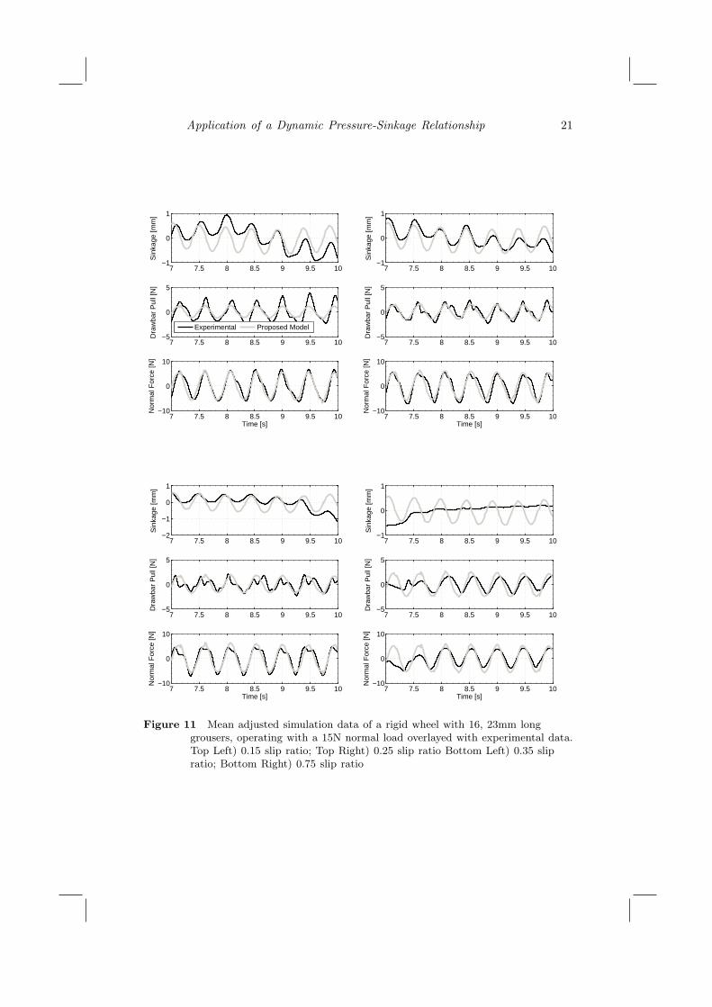
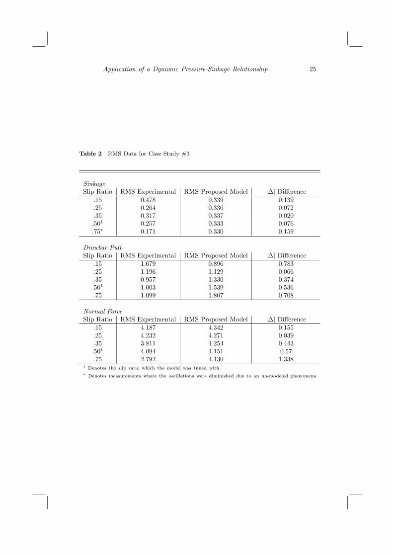
To further validated the predictive capabilities of the model, comparisonsfor slip ratios of 0.15, 0.25, 0.35 and 0.75 can be seen in Figure 11, whichpresents the data as mean-adjusted plots during steady-state operation so thatthe oscillations and contribution of the dynamic pressure-sinkage relationshipdescribed by Equation (20) be can be easily compared. The model parameters usedfor these cases were the same as those used to manually tune the model (Table1). The gradual entrance and exit of a grouser from the terrain is not consideredin this work and one will notice small discontinuities in the simulated data fromthe dynamic pressure-sinkage model in the presented data. The root mean squared(RMS) data comparing the simulated and experimental work is presented in Table2 along with the absolute difference or delta between these two calculations. TheRMS values were taken from the mean adjusted comparisons for the time periodsshown in Figures 10 and 11. The RMS values indicate reasonable and consistentresults when compared to the time history results of Figures 10 and 11.

Figure 11 shows that the dynamic model is able to accurately predict theoscillations in the sinkage, drawbar pull and normal force for all cases exceptfor the 0.75 slip ratio case. At this high slip ratio the wheel is excavating theterrain and the sinkage becomes smoother. When the excavation increases one willalso notice that the RMS delta (difference) values (Table 2) increase for all threemeasurements. When examining the normal load RMS delta for the 0.75 slip ratio


case, the model is over predicting the amplitude and the resulting RMS delta is1.338. A possible explanation for this reduction in the experimental oscillationamplitude is that, at such high slip ratios, the terrain does not come to rest beforethe next grouser comes into contact with it resulting in a more continuous flowof sand material. Such as fluidization, which can occur when a granular materialis excited by small displacements through vibration or other means, cause themacroscopic property of the granular system to change from a solid to a fluidJaeger and Nagel (1992). This fluidization phenomena is not accounted for in thecurrent terramechanic model.

The next case study investigates the ability of the new dynamic model topredict oscillations in the sinkage, drawbar pull and normal force when the grouserlength is reduced from 23mm to 10mm.

2.4 Case Study #4: SWTB Experiments – Grouser Length

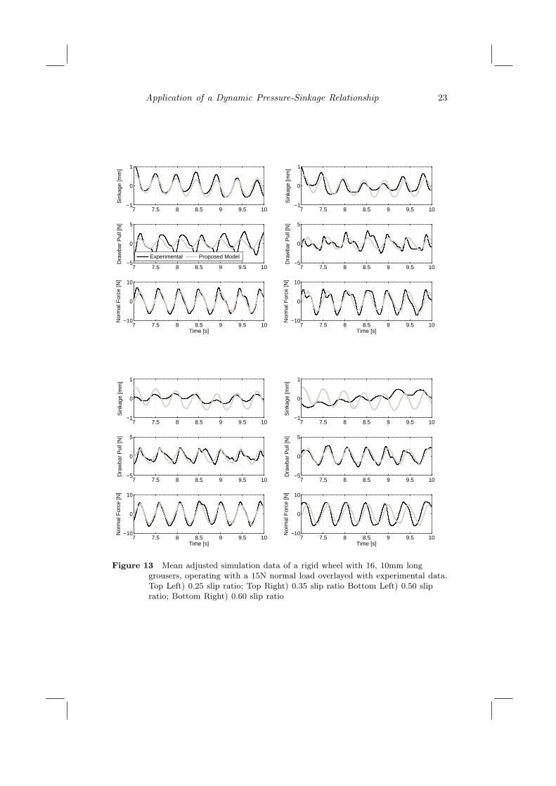
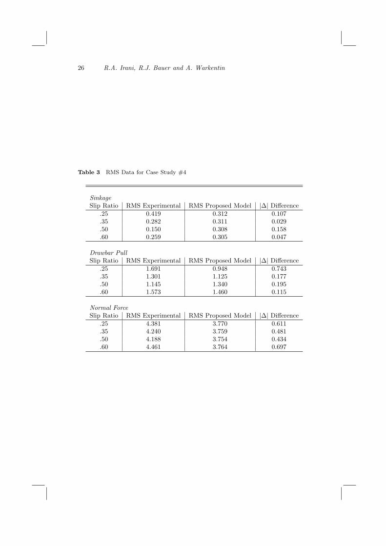
Building on the previous case study, SWTB experiments were carried out usinga 16 grouser wheel which had the length of each grouser reduced from 23mm to10mm. Figure 13 plots the resulting mean-adjusted experimental and simulatedvalues for sinkage, drawbar pull and normal force as a function of time for slipratios of 0.25, 0.35, 0.50 and 0.60. The values used for this case study were, again,kept the same as those used to originally tune the model (Table 1). For this casestudy, Table 3 presents the RMS data for the experimental and simulated data.The table also presents the difference or delta between these two calculations. TheRMS values were taken from the mean adjusted comparisons for the time periodsshown in Figure 13 and indicate reasonable and consistent results when comparedto the time history data of Figure 13.

One can see from Figure 13 that, for the 0.25 and 0.35 slip ratio cases, theoscillations in all of the measured data is accurately predicted by the model. Asobserved in the previous section, at the higher slip ratios, particularly 0.60, themodel begins to lose its predictive capability for the oscillations in the sinkage.This result is expected based on the previous Case Study. As the wheel beginsto spin for longer periods of time in the same location, the wheel appears tocontinuously excavate the surrounding terrain. Since the wheel lacks appreciableforward movement into undisturbed terrain, the grousers cause the sand in thevicinity of the wheel to be in constant motion. This fluidization phenomenaoccurring with high-slip conditions is not accounted for in the dynamic pressure-sinkage relationship.

2.5 Case Study #5: SWTB – Grouser Number

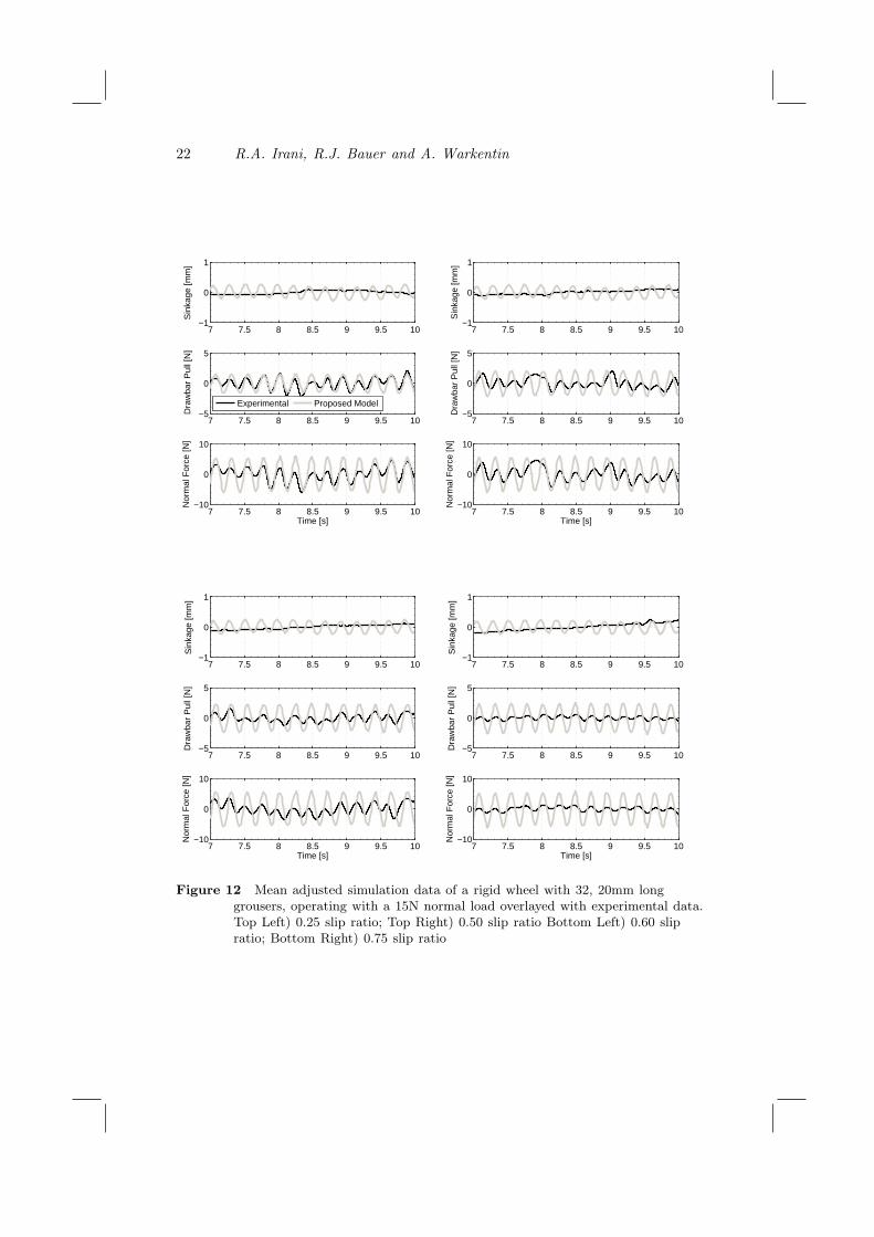
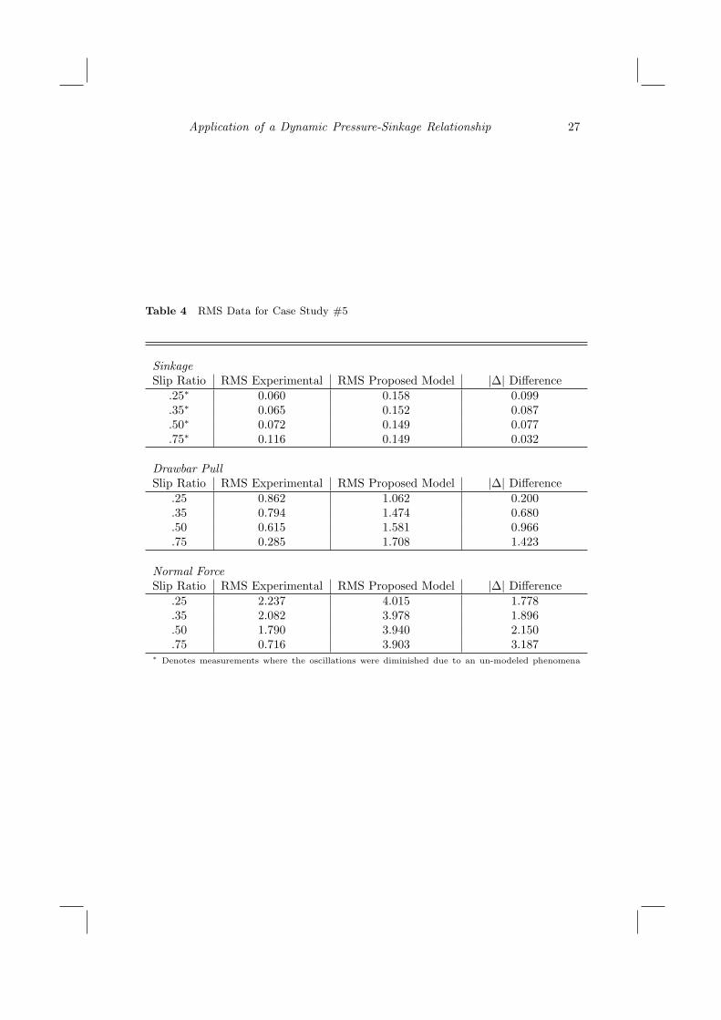
For this case study the number of grousers, each 10mm long, was increased from 16to 32, and SWTB experiments and corresponding model simulations were carriedout. Figure 12 show the resulting mean-adjusted overlay of experimental andsimulated sinkage, drawbar pull and normal force plotted as a function of time forslip ratios of 0.25, 0.50, 0.60 and 0.75. The model parameters used for this casestudy were again set using the original tuning case (Table 1). One will notice fromFigure 12 that all of the experimental sinkage results, including those at the lowestslip ratio tested, did not present noticeable oscillations. This observation, given


the resulting increase in flow of sand grains caused by a doubling of the numberof grousers, can likely be attributed to the same fluidization phenomena whichoccurred in the previous two test cases. When examining the drawbar pull resultsin Figure 12 one can see that the results are reasonable for slip ratios of 0.25, 0.50and 0.60; however, at a slip ratio of 0.75 the oscillations become less significant inall three measured signals — again, likely due to fluidization as the sand grainsexperience a constant flow at these higher slip ratios.

The RMS data comparing the simulated and experimental work is presented inTable 4. The RMS values show a large over prediction from the model, especiallyin the normal force results where the minimum and maximum deltas are 1.778 and3.187, respectfully. One will notice that the delta RMS values of the sinkage resultsare very small, suggesting that the model is accurately predicting the amplitudeof the oscillations. However, examining the time history data in Figure 12 onewill see that there are no oscillations in the sinkage measurements. Therefore,examining only the RMS values as a measure of accuracy can be misleading. Ifone examines Figure 12, the experimental data has some natural variation or driftfor all slip ratios during the time period shown in the figure. The amplitude ofthe drift is very close to the amplitude of the model-predicted oscillations. SinceRMS calculations are independent of phase and frequency, one cannot rely solelyon the delta RMS data to conclude if the results are accurate, reasonable or valid.To correctly interpret the RMS results, one must also examine the time historyresponse to conclude if excessive excavation is occurring.

3 Conclusions

As a result of the case studies presented in this work, the authors have shown thatthe dynamic pressure-sinkage model described by Irani et al. (2010a, 2011a) shouldonly be implemented when there is sustained slippage and positive drawbar pullfor smooth wheel cases. Case studies which varied the number and length of thegrousers on a wheel demonstrated that the model is able to reasonably captureand predict the dynamic oscillations observed in the drawbar pull and normal forcemeasurements using only one tuning condition (16, 23mm long grousers operatingat a slip ratio of 0.50 and a normal load of 15N). Under high-slip conditions orwhen the number of grousers on a wheel is relatively high, there appears to bean unaccounted for fluidization phenomena which reduces the amplitude of theobserved oscillations in the sinkage. Also, RMS data should be used in conjunctionwith time history data to ensure the numeric quantification is appropriate andmeaningful.

Further work needs to be carried out to explore the full potential andlimitations of the dynamic pressure-sinkage relationship, such as side slip effects,terrain variations and its application in terrain parameter estimation.

FIGURES


0 5 10 150

10

20

30

Sin

kage

[mm

]

0 5 10 150

10

20

30D

raw

bar

Pul

l [N

]

0 5 10 150

10

20

30

Nor

mal

For

ce [N

]

Time [s]

Figure 1 Experimental data of a rigid wheel with 16, 23mm long grousers, operatingat 0.50 slip and a 15N normal load

Figure 2 Forces and stress acting on a wheel which a typical terramechanic modelcalculates


Figure 3 Active and Passive stress zones on a wheel when grousers are present

Input model

constraints

and initial

sinkage

Compute and the

current location of

grousers based on the

initial sinkage

Are

Grousers in contact

with soil?

Calculate f and r.

Compute the mean

value of the passive

stresses for the

grousers in contact

with the soil.

Calculate A

Calculate the

contact length lc

and A . Combine

A and A

Determine the

normal stress and

shear stress and

numerically integrate

along the contact

length to determine

Fz and Fx

A is zero. Calculate f and r.

Calculate the contact length lc

and A Determine ( ) and

( ) and numerically integrate

along the contact length to

determine Fz and Fx.

Compute the sum

of forces with the

added vertical

friction

Calculate the new

position of the

grousers based on the

new sinkage and time

Integrate vertical

acceleration to determine

sinkage values and

increment time

No

Yes

No Yes

t tmax

Figure 4 Flow chart of the algorithm implemented in MATLAB/Simulink


Figure 5 Micro rover at the end of a 6◦ slope climb


Figure 6 Tracks from the rear wheels of the micro rover


0.8 0.85 0.9 0.950

1

2

3

4

5

6

7

Slip ratio

Fre

quen

cy [r

ad/s

]

Experimental resultsFitted

ω = −30.04i + 29.77

R2 = 0.9998

Figure 7 Ripple Frequency vs slip ratio

−160 −140 −120 −100 −80 −60 −40 −20−200

0

200

400

600

800

1000

1200

1400

Str

ess

[kP

a]

Angular Position on Wheel [Deg]

Normal Stress, σShear Stress, τ

η = 0.95slip = 0.35

GrouserLocationt = t

o

t = t1

t = t2

t = t3

t = t4

t = t5

Figure 8 Normal and shear stress along the face of the wheel with active and passivestress added to the shear stress


Figure 9 Experimental equipment: Single wheel testbed (SWTB)


0 5 10 150

10

20

30

Sin

kage

[mm

]

0 5 10 150

10

20

30

Dra

wba

r P

ull [

N]

ExperimentalDynamic ModelClassic Model

0 5 10 150

10

20

30

Nor

mal

For

ce [N

]

Time [s]

Figure 10 Overlay of experimental data with the dynamic and classic models for arigid wheel with 16, 23mm long grousers, operating at 0.50 slip and a 15Nnormal load


7 7.5 8 8.5 9 9.5 10−1

0

1

Sin

kage

[mm

]

7 7.5 8 8.5 9 9.5 10−5

0

5

Dra

wba

r P

ull [

N]

7 7.5 8 8.5 9 9.5 10−10

0

10

Nor

mal

For

ce [N

]

Time [s]

Experimental Proposed Model

7 7.5 8 8.5 9 9.5 10−1

0

1

Sin

kage

[mm

]

7 7.5 8 8.5 9 9.5 10−5

0

5

Dra

wba

r P

ull [

N]

7 7.5 8 8.5 9 9.5 10−10

0

10N

orm

al F

orce

[N]

Time [s]

7 7.5 8 8.5 9 9.5 10−2

−1

0

1

Sin

kage

[mm

]

7 7.5 8 8.5 9 9.5 10−5

0

5

Dra

wba

r P

ull [

N]

7 7.5 8 8.5 9 9.5 10−10

0

10

Nor

mal

For

ce [N

]

Time [s]

7 7.5 8 8.5 9 9.5 10−1

0

1

Sin

kage

[mm

]

7 7.5 8 8.5 9 9.5 10−5

0

5

Dra

wba

r P

ull [

N]

7 7.5 8 8.5 9 9.5 10−10

0

10

Nor

mal

For

ce [N

]

Time [s]

Figure 11 Mean adjusted simulation data of a rigid wheel with 16, 23mm longgrousers, operating with a 15N normal load overlayed with experimental data.Top Left) 0.15 slip ratio; Top Right) 0.25 slip ratio Bottom Left) 0.35 slipratio; Bottom Right) 0.75 slip ratio


7 7.5 8 8.5 9 9.5 10−1

0

1

Sin

kage

[mm

]

7 7.5 8 8.5 9 9.5 10−5

0

5

Dra

wba

r P

ull [

N]

7 7.5 8 8.5 9 9.5 10−10

0

10

Nor

mal

For

ce [N

]

Time [s]


7 7.5 8 8.5 9 9.5 10−1

0

1

Sin

kage

[mm

]

7 7.5 8 8.5 9 9.5 10−5

0

5

Dra

wba

r P

ull [

N]

7 7.5 8 8.5 9 9.5 10−10

0

10N

orm

al F

orce

[N]

Time [s]

7 7.5 8 8.5 9 9.5 10−1

0

1

Sin

kage

[mm

]

7 7.5 8 8.5 9 9.5 10−5

0

5

Dra

wba

r P

ull [

N]

7 7.5 8 8.5 9 9.5 10−10

0

10

Nor

mal

For

ce [N

]

Time [s]

7 7.5 8 8.5 9 9.5 10−1

0

1

Sin

kage

[mm

]

7 7.5 8 8.5 9 9.5 10−5

0

5

Dra

wba

r P

ull [

N]

7 7.5 8 8.5 9 9.5 10−10

0

10

Nor

mal

For

ce [N

]

Time [s]



TABLES

Table 1 Summary of Parameters

Parameter Value Unit Comments

k′c 0 – Dimensionless cohesive modulusk′ϕ 20 – Dimensionless frictional modulus

K 0.036 m Shear deformation modulusn 1 – Sinkage exponentγ 13734 N/m3 Soil weight densitydγ 0.1× γ N/m3 Change in soil weight densityr 0.1 m Radius of wheelb 0.075 m Width of wheelη 1.35 – Rear of wheel sinkage relationshipϕ 28 deg Internal angle of frictionc 0 kPa Soil cohesionCf 800 Ns/m Viscous friction coefficientk′g 0.1 – Dimensionless grouser amplitude coefficientk′a 0.05 – Dimensionless density amplitude coefficient


Table 2 RMS Data for Case Study #3

SinkageSlip Ratio RMS Experimental RMS Proposed Model |∆| Difference

.15 0.478 0.339 0.139

.25 0.264 0.336 0.072

.35 0.317 0.337 0.020.501 0.257 0.333 0.076.75∗ 0.171 0.330 0.159

Drawbar PullSlip Ratio RMS Experimental RMS Proposed Model |∆| Difference

.15 1.679 0.896 0.783

.25 1.196 1.129 0.066

.35 0.957 1.330 0.374.501 1.003 1.539 0.536.75 1.099 1.807 0.708

Normal ForceSlip Ratio RMS Experimental RMS Proposed Model |∆| Difference

.15 4.187 4.342 0.155

.25 4.232 4.271 0.039

.35 3.811 4.254 0.443.501 4.094 4.151 0.57.75 2.792 4.130 1.338

1 Denotes the slip ratio which the model was tuned with

∗ Denotes measurements where the oscillations were diminished due to an un-modeled phenomena




.25 0.419 0.312 0.107

.35 0.282 0.311 0.029

.50 0.150 0.308 0.158

.60 0.259 0.305 0.047


.25 1.691 0.948 0.743

.35 1.301 1.125 0.177

.50 1.145 1.340 0.195

.60 1.573 1.460 0.115


.25 4.381 3.770 0.611

.35 4.240 3.759 0.481

.50 4.188 3.754 0.434

.60 4.461 3.764 0.697




.25∗ 0.060 0.158 0.099

.35∗ 0.065 0.152 0.087

.50∗ 0.072 0.149 0.077

.75∗ 0.116 0.149 0.032


.25 0.862 1.062 0.200

.35 0.794 1.474 0.680

.50 0.615 1.581 0.966

.75 0.285 1.708 1.423


.25 2.237 4.015 1.778

.35 2.082 3.978 1.896

.50 1.790 3.940 2.150

.75 0.716 3.903 3.187∗ Denotes measurements where the oscillations were diminished due to an un-modeled phenomena


References

Azimi A., Hirschkorn M., Ghotbi B., Kovecses J., Angeles J., Radziszewski P.,Teichmann M., Courchesne M., and Gonthier Y. (2010) Simulation-based roverperformance evaluation and effects of terrain modelling, In CASI AstronauticsConference ASTRO 2010, May 4-6 2010.

Apostolopoulos D. , Wagner M., Heys S. and J. Teza. (2003) Results of theinflatable robotic rover testbed. Technical Report CMU-RI-TR-03-18, CarnegieMellon University, June 2003.

Arvidson, R.E. and Bell III, J.F. and Bellutta, P. and Cabrol, N.A. and Catalano,J.G. and Cohen, J. and Crumpler, L.S. and Des Marais, D.J. and Estlin, T.A. andFarrand, W.H. and others (2010). Spirit Mars Rover Mission: Overview and selectedresults from the northern Home Plate Winter Haven to the side of Scamander crater.J. Geophys. Res, 115, 2010.

M. G. Bekker (1969). Introduction to terrain-vehicle systems. University of MichiganPress, Ann Arbor.

Holtz R.D. and Kovacs W.D. (1981). An introduction to geotechnical engineering,volume 733. Prentice-Hall.

Ishigami G., Miwa A., Nagatani K., and Yoshida K. (2007). Terramechanics-based modelfor steering maneuver of planetary exploration rovers on loose soil. Journal of FieldRobotics, 24(3):233250.

Ishigami G. Terramechanics-based Analysis and Control for Lunar/ PlanetaryExploration Robots. Phd Thesis, Tohoku University, Department of AerospaceEngineering, March 2008.

Jaeger H.M. and Nagel S.R. (1992). Physics of the granular state. Science,255(5051):1523.

Karafiath L.L. and Nowatzki E.A. (1978). Soil Mechanics for Off-Road VehicleEngineering. Clausthal Germany: Trans Tech Publications.

Lyasko M. (2010). LSA model for sinkage predictions. Journal of Terramechanics,47(1):1-19.

Meirion-Griffith G. and Spenko M. (2011). A modified pressure sinkage model for small,rigid wheels on deformable terrains. Journal of Terramechanics, 48(2):149 155.

Irani R., Bauer R., Warkentin A. (2011a). A dynamic terramechanic model for smalllightweight vehicles with rigid wheels and grousers operating in sandy soil. Journalof Terramechanics, 48(2): 307-318.

Irani R., Bauer R., Warkentin A. (2011). Dynamic terramechanic model for grouserwheels on a planetary rover in sandy soil. In CANCAM, 2011. Vancouver, BritishColumbia.

Irani R., Bauer R., Warkentin A. (2010b). Modelling a single-wheel testbed for planetaryrover applications. In Third Annual Dynamic Systems and Control Conference, 2010.Cambridge, Massachusetts.

Irani R., Bauer R., Warkentin A. (2010a). Design of a single-wheel testbed andpreliminary results for planetary rover applications. In The Canadian Society forMechanical Engineering Forum 2010. Victoria, British Columbia.

Reece A.R. Principles of soilvehicle mechanics. Proceedings of the Institution ofMechanical Engineers, Automobile Division, 180(1965):4566.

Wong J. Y. (2001). Theory of ground vehicles. John Wiley, New York.

Wong J.Y. (2010). Terramechanics and Off-Road Vehicles. Butterworth-Heinemann, 2edition.


Hanamoto B. and Janosi J. (1961). The analytical determination of drawbar pull as afunction of slip for tracked vehicle in deformable soils. In 1st Int. Conf. on Terrain-Vehicle Systems, Torino, Italy.