Antialiasing

CSE167: Computer Graphics

Instructor: Steve Rotenberg

UCSD, Fall 2006

Texture Minification

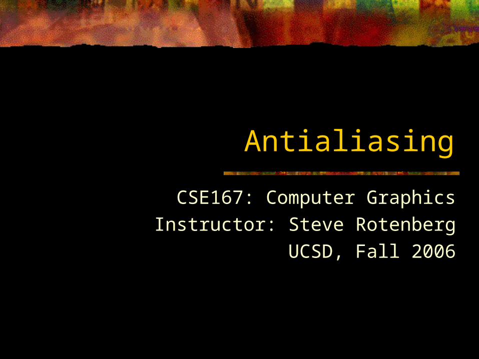
Consider a texture mapped triangle Assume that we point sample our texture

so that we use the nearest texel to the center of the pixel to get our color

If we are far enough away from the triangle so that individual texels in the texture end up being smaller than a single pixel in the framebuffer, we run into a potential problem

If the object (or camera) moves a tiny amount, we may see drastic changes in the pixel color, as different texels will rapidly pass in front of the pixel center

This causes a flickering problem known as shimmering or buzzing

Texture buzzing is an example of aliasing

Small Triangles

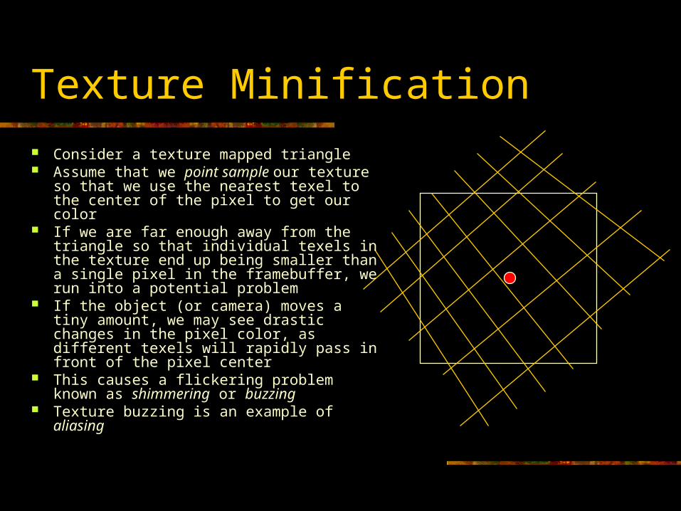
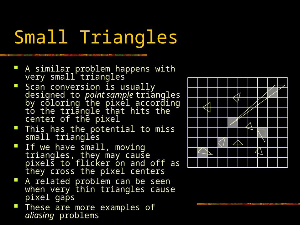
A similar problem happens with very small triangles

Scan conversion is usually designed to point sample triangles by coloring the pixel according to the triangle that hits the center of the pixel

This has the potential to miss small triangles

If we have small, moving triangles, they may cause pixels to flicker on and off as they cross the pixel centers

A related problem can be seen when very thin triangles cause pixel gaps

These are more examples of aliasing problems

Stairstepping

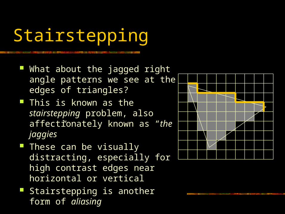
What about the jagged right angle patterns we see at the edges of triangles?

This is known as the stairstepping problem, also affectionately known as “the jaggies”

These can be visually distracting, especially for high contrast edges near horizontal or vertical

Stairstepping is another form of aliasing

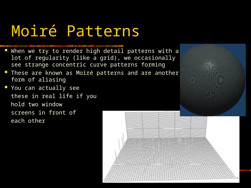
Moiré Patterns When we try to render high detail patterns with a lot of

regularity (like a grid), we occasionally see strange concentric curve patterns forming

These are known as Moiré patterns and are another form of aliasing

You can actually see

these in real life if you

hold two window

screens in front of

each other

The Propeller Problem

Consider an animation of a spinning propeller, that is rendering at 30 frames per second

If the propeller is spinning at 1 rotation per second, then each image shows the propeller rotated an additional 12 degrees, resulting in the appearance of correct motion

If the propeller is now spinning at 30 rotations per second, each image shows the propeller rotated an additional 360 degrees from the previous image, resulting in the appearance of the propeller sitting still!

If it is spinning at 29 rotations per second, it will actually look like it is slowly turning backwards

These are known as strobing problems and are another form of aliasing

Aliasing

These examples cover a wide range of problems, but they all result from essentially the same thing

In each situation, we are starting with a continuous signal We then sample the signal at discreet points Those samples are then used to reconstruct a new signal, that is

intended to represent the original signal However, the reconstructed signals are a false representation of the

original signals In the English language, when a person uses a false name, that is

known as an alias, and so it was adapted in signal analysis to apply to falsely represented signals

Aliasing in computer graphics usually results in visually distracting artifacts, and a lot of effort goes into trying to stop it. This is known as antialiasing

Signals

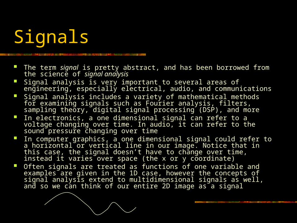
The term signal is pretty abstract, and has been borrowed from the science of signal analysis

Signal analysis is very important to several areas of engineering, especially electrical, audio, and communications

Signal analysis includes a variety of mathematical methods for examining signals such as Fourier analysis, filters, sampling theory, digital signal processing (DSP), and more

In electronics, a one dimensional signal can refer to a voltage changing over time. In audio, it can refer to the sound pressure changing over time

In computer graphics, a one dimensional signal could refer to a horizontal or vertical line in our image. Notice that in this case, the signal doesn’t have to change over time, instead it varies over space (the x or y coordinate)

Often signals are treated as functions of one variable and examples are given in the 1D case, however the concepts of signal analysis extend to multidimensional signals as well, and so we can think of our entire 2D image as a signal

Sampling

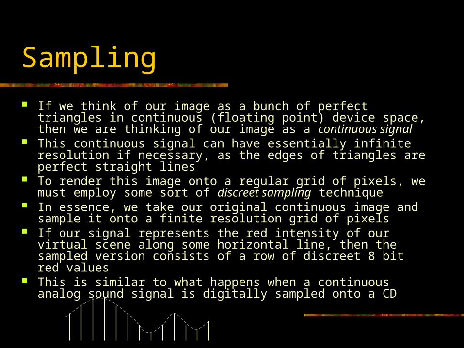
If we think of our image as a bunch of perfect triangles in continuous (floating point) device space, then we are thinking of our image as a continuous signal

This continuous signal can have essentially infinite resolution if necessary, as the edges of triangles are perfect straight lines

To render this image onto a regular grid of pixels, we must employ some sort of discreet sampling technique

In essence, we take our original continuous image and sample it onto a finite resolution grid of pixels

If our signal represents the red intensity of our virtual scene along some horizontal line, then the sampled version consists of a row of discreet 8 bit red values

This is similar to what happens when a continuous analog sound signal is digitally sampled onto a CD

Reconstruction

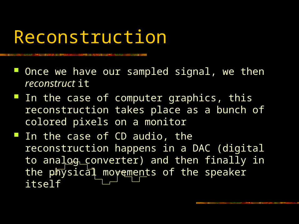
Once we have our sampled signal, we then reconstruct it In the case of computer graphics, this reconstruction

takes place as a bunch of colored pixels on a monitor In the case of CD audio, the reconstruction happens in a

DAC (digital to analog converter) and then finally in the physical movements of the speaker itself

Reconstruction Filters

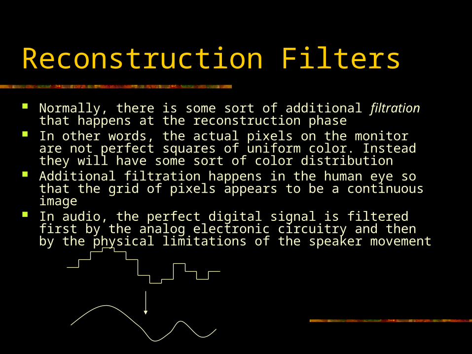
Normally, there is some sort of additional filtration that happens at the reconstruction phase

In other words, the actual pixels on the monitor are not perfect squares of uniform color. Instead they will have some sort of color distribution

Additional filtration happens in the human eye so that the grid of pixels appears to be a continuous image

In audio, the perfect digital signal is filtered first by the analog electronic circuitry and then by the physical limitations of the speaker movement

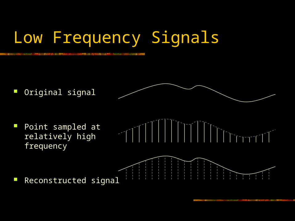
Low Frequency Signals

Original signal

Point sampled at relatively high frequency

Reconstructed signal

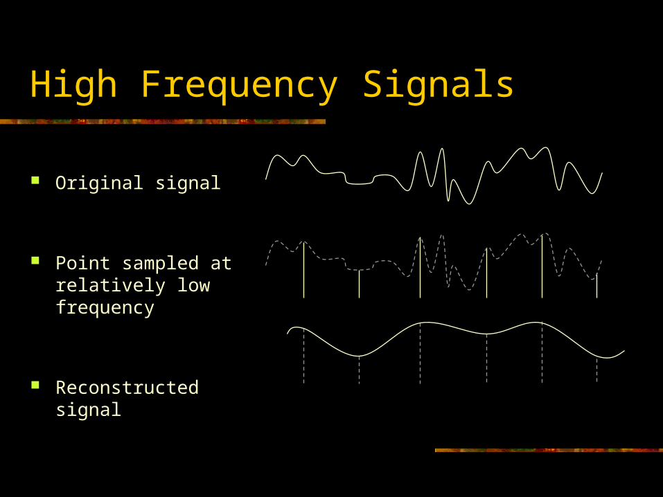
High Frequency Signals

Original signal

Point sampled at relatively low frequency

Reconstructed signal

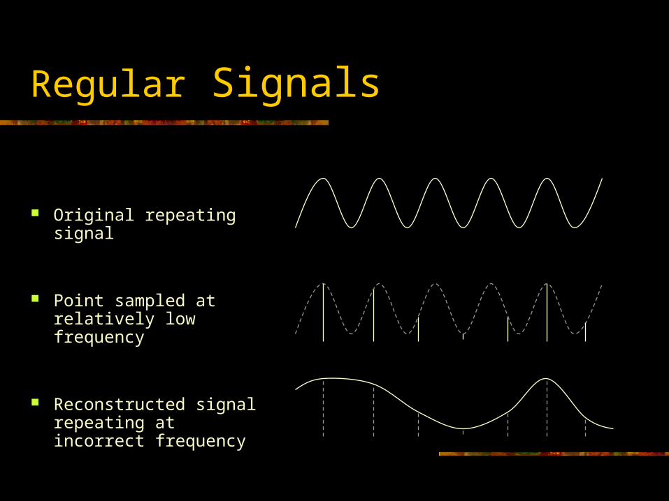
Regular Signals

Original repeating signal

Point sampled at relatively low frequency

Reconstructed signal repeating at incorrect frequency

Nyquist Frequency

Theoretically, in order to adequately reconstruct a signal of frequency x, the original signal must be sampled with a frequency of greater than 2x

This is known as the Nyquist frequency or Nyquist limit However, this is assuming that we are doing a

somewhat idealized sampling and reconstruction In practice, it’s probably a better idea to sample signals

at a minimum of 4x

Aliasing Problems

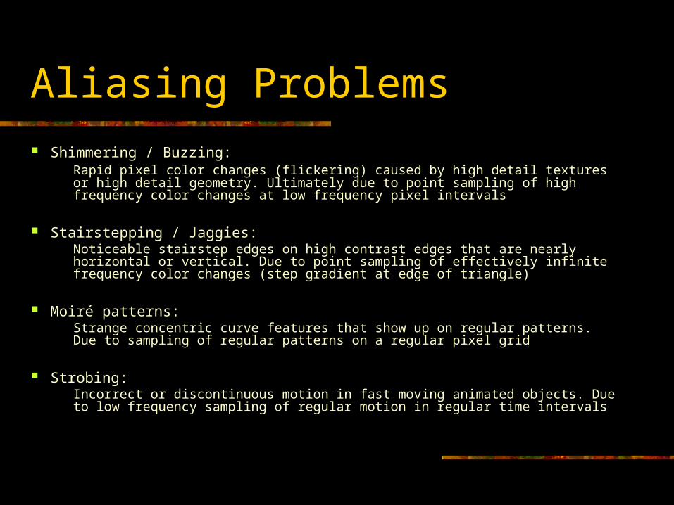
Shimmering / Buzzing:Rapid pixel color changes (flickering) caused by high detail textures or high detail geometry. Ultimately due to point sampling of high frequency color changes at low frequency pixel intervals

Stairstepping / Jaggies:Noticeable stairstep edges on high contrast edges that are nearly horizontal or vertical. Due to point sampling of effectively infinite frequency color changes (step gradient at edge of triangle)

Moiré patterns:Strange concentric curve features that show up on regular patterns. Due to sampling of regular patterns on a regular pixel grid

Strobing:Incorrect or discontinuous motion in fast moving animated objects. Due to low frequency sampling of regular motion in regular time intervals

Spatial / Temporal Aliasing

Aliasing shows up in a variety of forms, but usually those can be separated into either spatial or temporal aliasing

Spatial aliasing refers to aliasing problems based on regular sampling in space. This usually implies device space, but we see other forms of spatial aliasing as well

Temporal aliasing refers to aliasing problems based on regular sampling in time

The antialiasing techniques used to fix these two things tend to be very different, although they are based on the same fundamental principles

Point Sampling

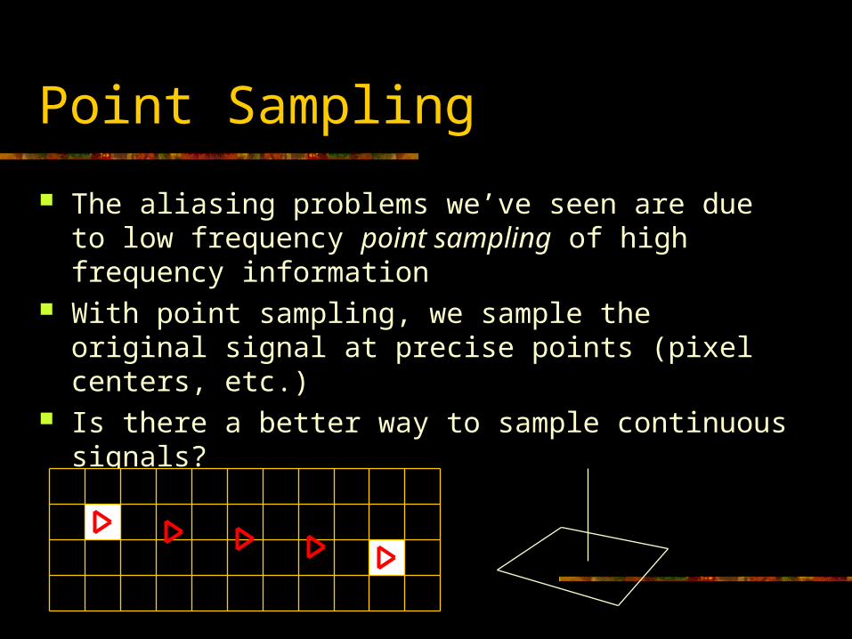
The aliasing problems we’ve seen are due to low frequency point sampling of high frequency information

With point sampling, we sample the original signal at precise points (pixel centers, etc.)

Is there a better way to sample continuous signals?

Box Sampling

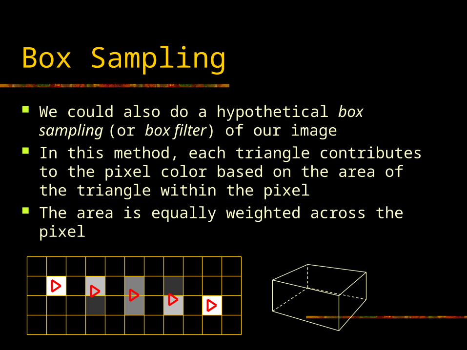
We could also do a hypothetical box sampling (or box filter) of our image

In this method, each triangle contributes to the pixel color based on the area of the triangle within the pixel

The area is equally weighted across the pixel

Pyramid Sampling

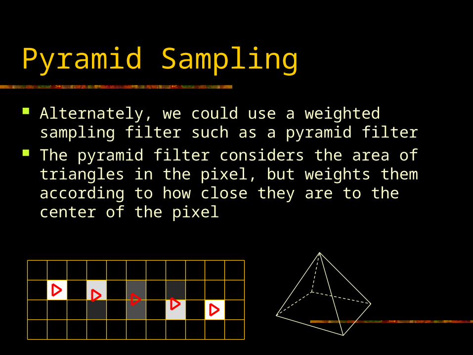
Alternately, we could use a weighted sampling filter such as a pyramid filter

The pyramid filter considers the area of triangles in the pixel, but weights them according to how close they are to the center of the pixel

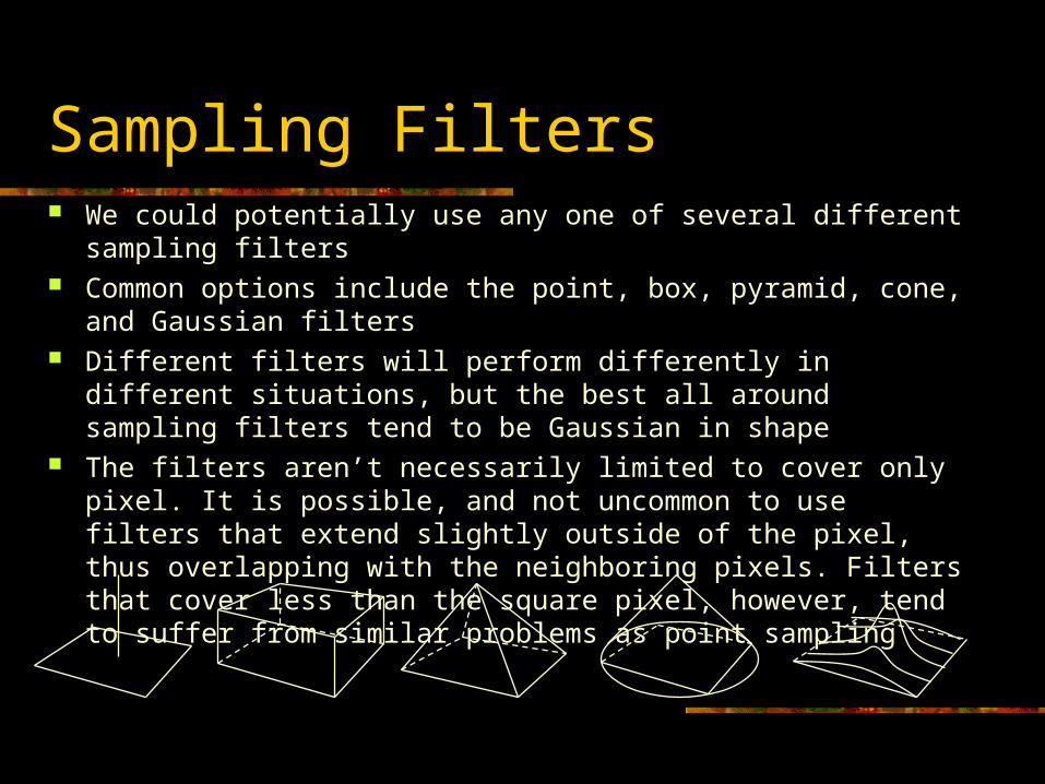
Sampling Filters We could potentially use any one of several different sampling filters Common options include the point, box, pyramid, cone, and

Gaussian filters Different filters will perform differently in different situations, but the

best all around sampling filters tend to be Gaussian in shape The filters aren’t necessarily limited to cover only pixel. It is

possible, and not uncommon to use filters that extend slightly outside of the pixel, thus overlapping with the neighboring pixels. Filters that cover less than the square pixel, however, tend to suffer from similar problems as point sampling

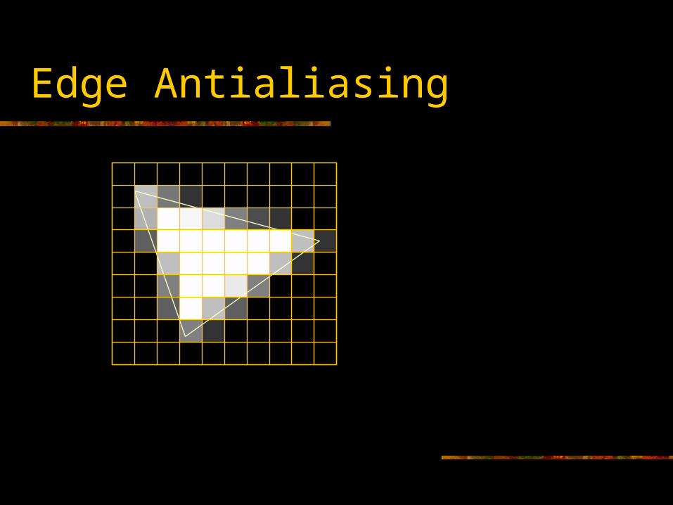
Edge Antialiasing

Coverage There have been several edge antialiasing algorithms proposed that

attempt to base the final pixel color on the exact area that a particular triangle covers

However, without storing a lot of additional information per pixel, this is very difficult, if not impossible to do correctly, in cases where several triangle edges cross the pixel

Making a coverage based scheme that is compatible with zbuffering and can handle triangles drawn in any order has proven to be a pretty impractical approach

Some schemes work reasonably well if triangles are sorted from back to front (distant to near), but even these methods are not 100% reliable

Supersampling

A more popular method (although less elegant) is supersampling

With supersampling, we point sample the pixel at several locations and combine the results into the final pixel color

For high quality rendering, it is not uncommon to use 16 or more samples per pixel, thus requiring the framebuffer and zbuffer to store 16 times as much data, and requiring potentially 16 times the work to generate the final image

This is definitely a brute force approach, but is straightforward to implement and very powerful

Uniform Sampling

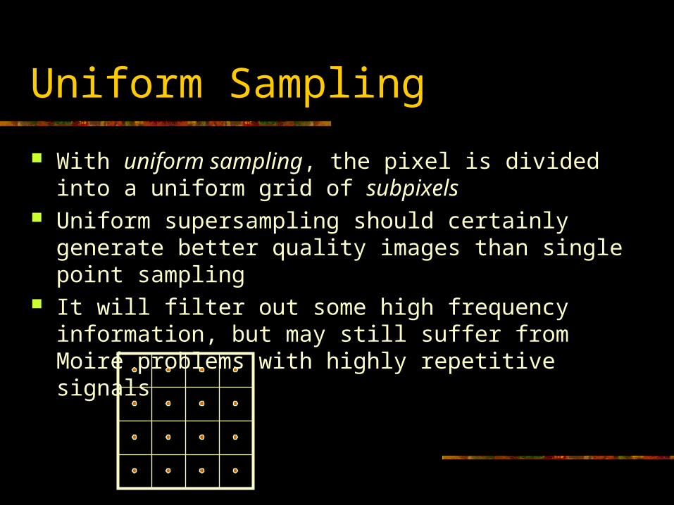
With uniform sampling, the pixel is divided into a uniform grid of subpixels

Uniform supersampling should certainly generate better quality images than single point sampling

It will filter out some high frequency information, but may still suffer from Moiré problems with highly repetitive signals

Random Sampling

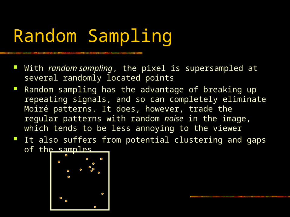
With random sampling, the pixel is supersampled at several randomly located points

Random sampling has the advantage of breaking up repeating signals, and so can completely eliminate Moiré patterns. It does, however, trade the regular patterns with random noise in the image, which tends to be less annoying to the viewer

It also suffers from potential clustering and gaps of the samples

Jittered Sampling

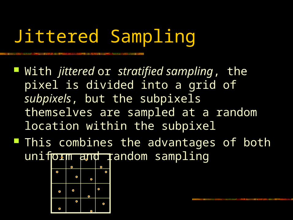
With jittered or stratified sampling, the pixel is divided into a grid of subpixels, but the subpixels themselves are sampled at a random location within the subpixel

This combines the advantages of both uniform and random sampling

Weighted Sampling

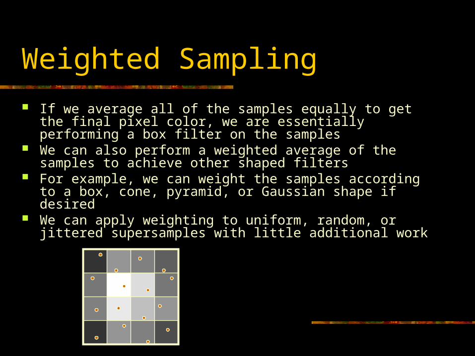
If we average all of the samples equally to get the final pixel color, we are essentially performing a box filter on the samples

We can also perform a weighted average of the samples to achieve other shaped filters

For example, we can weight the samples according to a box, cone, pyramid, or Gaussian shape if desired

We can apply weighting to uniform, random, or jittered supersamples with little additional work

Weighted Distribution

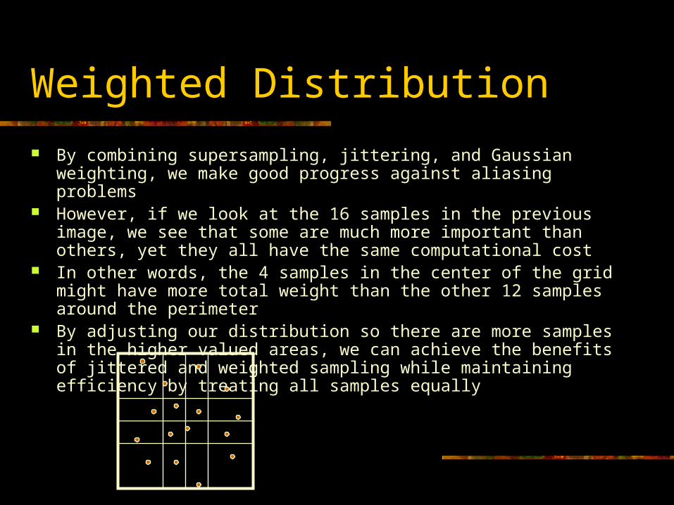
By combining supersampling, jittering, and Gaussian weighting, we make good progress against aliasing problems

However, if we look at the 16 samples in the previous image, we see that some are much more important than others, yet they all have the same computational cost

In other words, the 4 samples in the center of the grid might have more total weight than the other 12 samples around the perimeter

By adjusting our distribution so there are more samples in the higher valued areas, we can achieve the benefits of jittered and weighted sampling while maintaining efficiency by treating all samples equally

Adaptive Sampling

An even more sophisticated option is to perform adaptive sampling

With this scheme, we start with a small number of samples and analyze their statistical variation

It the colors are all similar, we accept that we have an accurate sampling

If we find that the colors have a large variation, we continue to take further samples until we have reduced the statistical error to an acceptable tolerance

Semi-Jittered Sampling

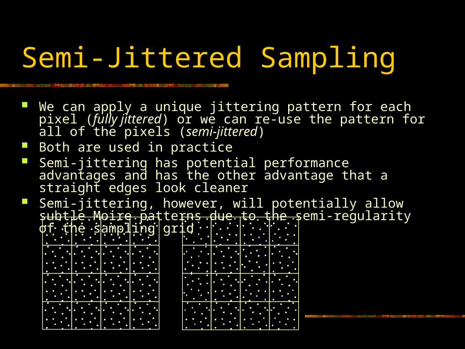
We can apply a unique jittering pattern for each pixel (fully jittered) or we can re-use the pattern for all of the pixels (semi-jittered)

Both are used in practice Semi-jittering has potential performance advantages and has the

other advantage that a straight edges look cleaner Semi-jittering, however, will potentially allow subtle Moire patterns

due to the semi-regularity of the sampling grid

Spatial Aliasing

Many of the spatial aliasing problems we’ve seen so far happen because of the regular grid of pixels

Using antialiasing techniques such as Gaussian weighted jittered supersampling can significantly reduce these problems

However, they can definitely add a large cost, depending on the exact implementation

Mipmapping & Pixel Antialiasing

We saw how mipmapping and other texture filtering techniques (such as elliptical weighted averaging) can reduce texture aliasing problems

These can be combined with pixel supersampling to achieve further improvements

For example, each supersample can be mipmapped, and these can be blended into the final pixel value, resulting in better edge-on behavior than mipmapping alone

Another hybrid approach is to compute only a single shading sample per pixel, but still supersample the scan-conversion and zuffering. This combines the edge antialiasing properties of supersampling and the texture filtering of mipmapping without the excessive cost of full pixel supersampling. Modern graphics hardware often uses this approach, resulting in a large increase in framebuffer/zbuffer memory, but only a small increase in cost

Temporal Aliasing

Properly tuned supersampling techniques address the spatial aliasing problems pretty well

We still may run into temporal aliasing or strobing problems when we are generating animations

Just as the spatial antialiasing techniques apply a certain blurring at the pixel level, temporal antialiasing techniques apply bluring at the frame level

In other words, the approach to temporal antialiasing is to add morion blur to the image

Motion Blur

Motion blur can be a tricky subject, and several different approaches exist to address the issue

The simplest, brute force approach is supersampling in time

Just as pixel antialiasing involves increasing the spatial resolution and blurring the results, motion blur involves increasing the temporal resolution and blurring the results

In other words, if we want to apply motion blur over a 1/30th second interval, we render several images spaced in time and combine them into a final image

If an object moves 16 pixels in one frame, then 16 supersample images (or even less) should be adequate to blur it effectively

Combining Antialiasing Techniques

We can even combine the two techniques without exponentially increasing the work (without requiring 16x16 times the work)

This can be done by rendering 16 supersamples total, each one spread in time and jittered at the pixel level

This overall approach offers a powerful foundation for other blurry effects such as: soft shadows (penumbrae), lens focus (depth of field), color separation (dispersion), glossy reflections, diffuse interreflections, etc.

Midterm Review

Traditional Graphics Pipeline

Transformation Lighting Clipping / Culling Scan Conversion Pixel Rendering

As we have seen several times, these stages are not always completely distinct and may overlap somewhat

They will also vary from implementation to implementation We will consider a pretty classic implementation of this approach

which is very similar to how things are done in GL

Triangle Rendering

Each triangle goes through the following steps:

1. Transform vertex positions & normals from object space to camera space2. Apply backface culling in camera space to determine if triangle is visible3. Compute lit vertex colors based on the unlit color, the vertex position & normal,

and the light positions/directions (lighting is computed in camera space)4. Compute dynamic texture coordinates if desired (such as environment mapping)5. Clip & cull triangle to view frustum. This may involve creating new (temporary)

verts and splitting the triangle into two or more6. Transform clipped verts into device coordinates, by applying perspective

transformation, perspective division, and viewport mapping7. Scan convert the triangle into a series of pixels. For each pixel compute

interpolated values for the color (rgba), depth (z), and texture coordinates (tx, ty)8. For each pixel generated in the scan conversion process, test the z value against

the zbuffer value. If the pixel is visible, compute the final color by looking up the texture color, combining that with the interpolated lit color and apply alpha blending if necessary

1. Transform to Camera Space

The vertex positions and normals that define the triangle get transformed from its defining object space into world space and then into camera space

These can actually be combined into a single transformation by pre-computing M=C-1·W

If our matrix is non-rigid (i.e., if it contains shears and/or scales), then the normals must be transformed by M-1T (which should be pre-computed) and then re-normalized to unit length

*

*

1*

1

n

nn

nMn

vMv

WCM

T

0

1

zyx

zyx

nnn

vvv

n

v

2. Backface Cull in Camera Space

We want to perform backface culling as early as possible, because we expect that it will quickly eliminate up to 50% of our triangles

We choose to do the test in camera space for simplicity, but it could also be done in object space with a little extra setup

Note that in camera space, the eye position e is located at the origin

invisible is ngle then tria00

0201

npe

ppppn

if

3. Compute Vertex Lighting

Next, we can compute the lighting at each vertex by using a lighting model of our choice. We will use a variation of the Blinn model

We perform lighting in camera space, so the camera space light positions should be precomputed

We loop over all of the lights in the scene and compute the incident color clgti for the light and the unit length direction to the light li. These are computed differently for directional lights and point lights (and other light types)

Once we have the incident light information from a particular light, we can use it to compute the diffuse and specular components of the reflection, based on the material properties mdif (diffuse color), mspec (specular color), and s (shininess)

Each light adds its contribution to the total light, and we also add a term that approximates the ambient light

sispecidifilgtambamb hnmlnmccmc **

4. Compute Texture Coordinates

Very often, texture coordinates are just specified for each vertex and don’t require any special computation

Sometimes, however, one might want to use dynamic texture coordinates for some effect such as environment mapping or projected lights

5. Clipping & Culling

The triangle is then clipped to the viewing frustum We test the triangle against each plane individually and compute the

signed distance dn of each of the 3 triangle vertices to the plane

By examining these 3 signed distances, we can determine if the triangle is totally visible, totally invisible, or partially visible (thus requiring clipping)

If an edge of the triangle intersects the clipping plane, then we find the point x where the edge intersects the plane

clipclipnnd npv

ba

ab

b

tt

dd

dt

vvx

1

6. Projection & Device Mapping

After we are done with all of the camera space computations (lighting, texture coordinates, clipping, culling), we can finish transforming the vertices into device space

We do this by applying a 4x4 perspective matrix P, which will give us a 4D vector in un-normalized view space

We then divide out the w coordinate to end up with our 2.5D image space vector

This is then further mapped into actual device space (pixels) with a simple scale/translation matrix D

vDv

v

vPv

w

z

w

y

w

x

D

v

v

v

v

v

v

4

7. Scan Conversion

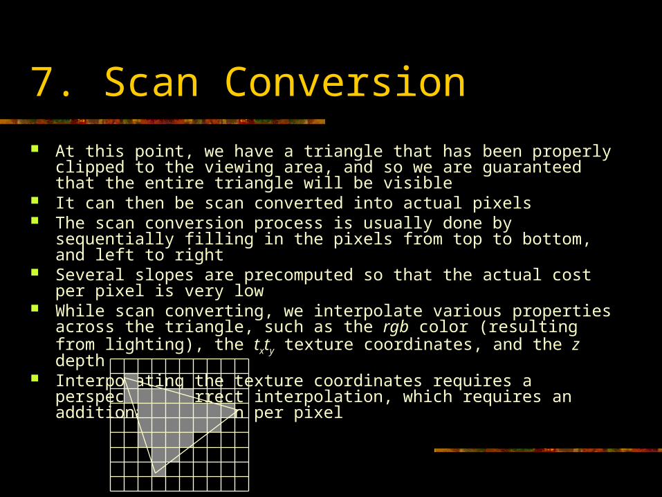
At this point, we have a triangle that has been properly clipped to the viewing area, and so we are guaranteed that the entire triangle will be visible

It can then be scan converted into actual pixels The scan conversion process is usually done by sequentially filling in the

pixels from top to bottom, and left to right Several slopes are precomputed so that the actual cost per pixel is very low While scan converting, we interpolate various properties across the triangle,

such as the rgb color (resulting from lighting), the txty texture coordinates, and the z depth

Interpolating the texture coordinates requires a perspective correct interpolation, which requires an additional division per pixel

8. Pixel Rendering

For each pixel generated in the scan conversion process, we have an interpolated depth value, texture coordinates, and a color, which are combined into the final color in the pixel rendering phase

The classic features that take place per pixel include: Test the zbuffer to see the pixel should be rendered at all Perform texture lookups (this may involve mipmapping, or bilinear

sampling, for example) Multiply the texture color with the Gouraud interpolated color (including

the alpha component) Blend this result with the fog color, based on the pixel z depth Blend this result with the existing color in the framebuffer, based on the

alpha value Write this final color, as well as the interpolated z depth into the

framebuffer/zbuffer