


Languages
Pages
Legal


An investigation intothe merits of fuzzylogic control versusclassical control
S.D.Florence
A project report submitted to the Faculty ofEngineering, University of the
Witwatersrand, johannesburg, in partialfulfilment of the requireme rts for the degree
of Master of Science in Engineering.
University of the WitwaterF-mnd, Johannesburg, July 1996.

Declaration
I declare that this project report is my own, unaided work. It is being submitted for
the Degree of Master of Science in Engineering in the University of the
Witwatersrand, Johannesburg. It has not been submitted before for any degree or
examination. in any other University.
~~. ----~.:-~--...-S.D.Florence

11
Abstract
Up to now the benefits and problems with fuzzy control have not been fully
identified and its role in the control domain needs investigation. The past trend has
been to show that a fuzzy controller can provide better control than classical
control, without examining what is actually being achieved. The aim in this project
report is to give a fair comparison between classical and fuzzy control. Robustness,
disturbance rejection, noise suppression" nonminimurn phase and dead time are
examined for both controllers. The comparison is performed through computer
simulation of classical and fuzzy controlled plant models. Fuzzy control has the
advantage of non-linear performance and the ability to capture linguistic
information. Translating quantitative information into the fuzzy domain is difficult;
therefore when the system is easily mathematically modelled and linear, classical
control is usually better. Which controller should be used depends on the
application, control designer and information available.

111
--...~-.----~---.----
Acknowledgements
I would like to thank:
• Dr. B. \Vigdorowitz fur his time, encouragement and supervision.
• Mandy and my family for their support and encouragement.

lV
---~.-----,-----
Table of Contents
Declaration ..•fi •• -s Q ••••• e •••••••••••••••••...................................... " ••••••••••••••••••••••••••• i
Abstract .•".~..•...••.••~f ..•••••••• " •• O ••••••••• O O •••••• CI t) •• ., •••••••• , ••••••••••••••••• 0 ••••••••••••• "
Acknowledgements <tCl •••••••••••••••••••••••••••.••••••••••• " * •• Q •••••••••••••••• ~ ••• iii
Table of Contents oo ••••••• ~ •••••• , •• " •••••••• o ••••• " ••••• O ~ SI •••••• iv
Li..st of Figures "................•..•.............. o.~ e .q ft •• o ",It ;:;,
List of Tables o u ••••••••••••• e x;i;
List of ..Symbols.. ...•.•..........•....... .,.......,...•.......................... o •••••••• tla •••••••••••• " •••••••••• xiv
1. Introduction "................•..... "•.....................................•.................. " 1
1.1 What is fuzzy control ? 8••••••••• " u •••••••••••• , ••••••••••••••••••••••••••••••••••• * ••••••••••••••• 1
1.2 Fuzzy control ..•.....•.....•.•..•.•..... e •••••• o••• , ~ 2
1.3 Problems and myths surrounding fuzzy logic ••.••••••..•••••••••••••••..••,•.••••••••.••••••••••••3
1.4 The aim of this Investigation, ".••.••..•.......••.•..•.••.•...•.•••••.•.••"u 6
1.5 Approach taken .0 •••••••••••••••••••••••••••• 8••••••••••••••••• " "' 7
2. Fuzzy logic concepts required in control u 9
2.1 Definition of a Fuzzy Logic System .0" filU ••• 9
202 Rationale for Fuzzy Logic " "'.It ••••••••• 13
2.3 Fuzzy Set Theory .....•.•......•.. oe •••••••••••••••••••••••••• o ••• o •••••••••••••••••••••••••••• fO •••• ~ ••••••••••• 11
2.3.1 Fuzzy Sets 11
2.3.2 Properties of Fuzzy Sets 12
v
2.3 ..3 Linguistic Variables 13
2.3.4 Fuzzy Numbers 14
2.3.5 Membership Functions , 15
2.3.6 Operations on Fuzzy Sets 18
2.3.G.l U'1:011 and Intersection 18
2.3.6.2 Complement. 21
2.3.7 Fuzzy Relations and Compositions " 22
2.3. 7.1 Fuzzy Relations 22
2.3.7.2 Fuzzy Compositions 23
21P4 Fuzzy Logic Systems a •••• ~••••••••••••••• o •••••••••• ~••••• , ' 0 26
2.4.1 Input Fuzziflcation 27
2.4.2 The Rules 27
2.4.2.1 Fuzzy Propositions " 27
2.4.2.2 Fuzzy Rules 28
2.4.3 Fuzzy Inference Scheme 29
2.4.3.1 Inference ofa single rule 29
2.4.3.2 Inference ofa rule base 30
2.4.4 Defuzzification 35
2.4.4.1 Maximum Defuzzifier ,,, 35
2.4.4.2 Mean of Maxima Defuzzifier 35
2.4.4.3 Centroid or Centre-of-Gravity Defuzzifier .35
2.4.4.4 Singletons 36
2.5 Fuzzy Systems as Universal Approximators 39
2..6 Adaptive FIIZZY Control 0." •• ' ••••• 0••••••••• 40
2.6.1 Self-organising fuzzy control 40
2.6.2 Fuzzy relations as associative memories .41
2.6.3 Adaptation by fuzzy supervisors 41
2.6.3.1 Fuzzy PID control 41
2.6.3.2 Adaptive fuzzy expert controller'"? 42
2.6.4 Gradient-descent adaptation 42
2.7 Summary .11•• 0 ••••••••• ('••••••••••••••••••• " •••••• ' , ••••• "•••••••••••• oe " •••••••• f'. 42
3. Aspects of fuZZ)' and classical control. ou " o 44
3.1 Definitions •••.••.I!I •••••••••••••••••••••••• e- ••••••• ot' •••••••••••••••••••••• 0 •••••• 11 ••••••• 8 •••• 11 ••••••••••••••••••••• 44

Vi
------~--
3. J.l Classical Control , " 44
3.1.2 Fuzzy Control 45
3.2 l"hE.classical control loop .. e •••••• ,; •••• G ••••••••••• ( •••••• .lI •••••••• O e •••••• 01' ••••• 46
3.2.1 Reason for feedback " 46
3.2.2 Structure ofa linear 81S0 feedback loop .47
3.2.3 Limitations of classical control.., 48
3.2.4 Background to QFf control 49
3.3 Control Aspects 1(1 •••• " •••••• "" ••••••••• 0••••••••••••••••••••• e ••••••••••• ., •••••• 4- ••••••••••••••••••••••• 49
3.3.1 Stability , 49
3.3.1.1 QFr stability 50
3.3.1.2 Fuzzy stability 50
3.3.2 Disturbance rejection 52
3.3.2.1 QFr design 52
3.3.2.2 Fuzzy design 52
3.3.3 Sensor noise suppression 53
3.3.3.1 QFT control 53
3.3.3.2 Fuzzy control. 54
3.3.4 Parameter variation 54
3.3.4.1 QFr control. 55
3.3.4.2 Fuzzy control. 55
3.3.S Unmodelled dynamics 56
3.3.5.1. OFT control. 56
3.3.5.2 Fuzzy control. 56
3.3.6 Non-minimum phase plants 57
3.3.7 Dead time. 58
3.3.8 Saturation 58
3.3.9 Temporal determinism 59
:' .3.1 ()Reliability and safety 59
3.4 Applications of fuzzy control ".••••.•"'."..•o•• "',.•• ~.o ••••• " •••••••••••••••••••• " " ••• 0•••••••••• 603.4.1 History of fuzz), control. 60
3.4.2 Summary of some applications of fuzzy control., 61
3.5 Qualitative versus quantitative knowledge •........... , 64
3.5.1 Tools available for fuzzy control 66
3.6 Approach to comparing control systems u•••••••••~ '"66

\;
3.1 Summary ,. e c •• & O .. ~ ••• O ••••••••••• If •••••••••• $ O ••.................. .,c.t! i:I " •••••••••• ,j. 67
4a Plant Mo(lelling .•...e •••• e e •• !J •••••••• .,..lfo ••• 9.o •••• ~ •••••••••••••.••••• <I ~ •••••• 4 •• 68
4.1 Introduction ........•••.•o~ •••• ~·•••••••• e e •••••••••• o ".-D •• "••••••••••••••••••••••••• "'••• II ••••••••••• " 1, ••• 68
4.2 Servo. motor system c•••• O••••••• c.O •••••••• O•••••••••• c.~ •••••••• (I •.............. e•••••••••••• $ ••••• I.~ •• 694.2.1 Rationale 69
4.2.2 Assumptions , , 70
4.2.3 Limitations ' 70
4.2.4 Mathematical Model 71
4.2.5 Physical Parameters 72
4.2.6 Final Model 72
4.3 CSTR pj''9.nt model "••••.•••.••••••••..•••••••o • ., •• q e ••••• e •••••••••••••• 734.3.1 Rationale 73
4.3.2 Assumptions 74
4.3.3 Mathematical Model 74
4.3.4 Parameter Values 78
4.3.~ Linear Model 78
4.4 Tank System .•...~ o., ••• " •••• ~••••••• c ••••• ~ 794.4.1 Rationale 79
4.4.2 Assumptions 80
4.4.3 Limitations 80
4.4.4 Mathematical Model 80
4.4.5 Physical Parameters 81
4.4.6 Linearised plant 81
4.5 Miscellaneous plants " e.u "•••••••••••••••••••••••••••••• 82
4.6 Summary ...•........•.•..•........•.......•....•.. ~•.... (I ••••••••••••••••••••• 0 ., 82
5. Controller design and comparison 0 ••••••••••••• " •••••• 0 ••••• e •••••••••••• 11 ••••••• " •• ft 84
5.1 Controller design approach , 845.1.1 QFT design 85
5.1.2 Fuzzy design 85
5.,2 Controller specification and design J.u ••••• u ••••••••• ._ u ••••••••••• 87
5.2.1 Servo motor 88

Vl11
5.2.1.1 Plant model . , 88
5.2.1.2 ()}<"Tspecifications and design , 88
5.:!. U Fuzzy specifications and design , 89
5.2.2 CSTRpiant. - _ 90
5.2.2-1 Plant model _ , 91
5.2.2.2 QFf design , __ ,.91
5.2.2.3 Fuzzy Design _ _ 93
5.2.3 T!.\nksystem , __ _ 94
5.2.3.1 Plant model 94
5.2.3.2 QFf design _ 94
5.2.3.3 Fuzzy control - _ _ " 95
5.3 Controller design and comparison for specific aspects of plants .....• o 95
5.3.1 Non-minimum phase plant. _.. 9E
-7_3.2 Highly non-linear plant _,. 99
5.33 Hybrid control ofa first order plant with dead time 99
5.4 Simulatics comparisons., ...•.•..•••.u.~ •••• ('•••••• ~••••• o "•••••••••••• 103
5.4.1 Tracking , 104
5.4.2 Disturbance rej::ction 107
5.4.3 Noise suppression .._ 109
5.4.4 Unmodelled dynamics'model variation "' 111
5.4, S Non-minimum phase 112
5.4.6 Dead time , 112
5.5 Design Comparison IP ••••• ~t:e ••• ' ••••••••••• IIt ••••••••• e (:0 ••••••••••••••• " ••••••• 114
5.6 Advantages and disadvantages of fuzzy control., 118
5.7 Summary '•..0 0•••••• 122
6. Conclusion ., ".. It ••••••••• " 0- •••••••••• 1' •••••••••••• " •••••• 0 •• ,.., 124
6.1 Future research " (1 "' 127
Appendix A : Model parameters o •• o ••••••• ".,. co•• ,UG •••••••••••••••••••••••• " ••••• 128
A.t Servo motor " , " G••••• e •••••• ~•••••••••• ~•••••••••••••••• O.O •• 128
A.2 CSTR e , •••••••••••••••••••••• o •••••••••• " •••••••••••••• 0.6- •••••••••••••••••••• e ••••••••••• "010 •• 128
AII3 Tank, .•.••••....••.•.o••••• e •••••• ".o •••••••••• tIo ••••••••••••••••••••• ,· •••••• 111 ••••••••••••••••• 0 131

-----~---
Appendix B : Block Diagrams "..•..o••••• It ••••• <.I ,.~e ••• «> •••••• " 132
B.I Servo motor .••..•.•.•.•••.•." 11 ••• " •••••••••••••••••••••••••••••• " ••••••••••••••••••••• ot".fil' •••••• "'" ••••• 132
B.2 CSTR .." tI c; ........................•••••• , o, "••••• e••••••••••••••••••••••••••• 134
C.3 Tank. o " ••••••••••••• ¢••••••••••••••••••• 9: •••••••••••• -00 ••• , ••••••••••••••••••••••• 1;1 ••••••••• 139
C.4 Nonminimum phase plant "'" c. •••• e ••••••••••••••• "••••••••••••••• 141
C.S First order system with dead time lIoo"•••••••••••• e ••••• u , •• u 142
Appendix c: Controllers .•...~."'.•....•..•....•.•.... c. ••••••••••••• 9.,,•• .,•••••••••••••••••••••••• 11 •••••••• 143
e.l QFTcontrollers ."'., O fllI •••• :t.~•• oo ••••••••• "IIo•••••••••• II O••••• Q •• ~ ••••••••••••••• i~3
C.I.l Servo motor 143
C.l.2 CSTR 144
C.l.3 Tank 145
c.z Fuzzy controllers v •••••• " ~ e ••••••••••••• G ••• " •• ~ ••••••••••••••••••• 146
C.2.! Servo motor 147
C.2.2 CSTR 148
C.2.3 Tank 148
C.2.4 Non-minimum phase 149
Cl!'3Hybrid Controller ,,~ O ••••••••••• 8 ••••••••••••••••••••••••••••••• ', ••••••••••••••••••••••• lSIC.3.1 Classical 151
C.3.2 Fuzzy 152
Appendix D ':MATJ...,AB@ Co{le.•••~....•.•. o ••••••••••••••••••••••••••••••••••••••• , 0 •• 153
D.I Servo motor e e •••••••••••••••••••• e ••• o••• "••• " "••••••••••••• ~•••••••• t -1' 153
D.l.1 servo_tf.m 153
D.1.2 pmap s.m 154
D.1.3 qft_serv.m 159
D.2 CSTR l ••••••••••••• ., ••••••• e •••••••••••••••••••••• O •••• ~ e ••••• " .....................•••••• e 163
D.2.l ccurve.m 163
D.2.2 lin_cstr.m 166
D.2.3 i__cstr.m 173
D.2.4 qft_.cstr.m 176

x---.--------------~---~~---.---
List of Figures
Figure 2·,1 : Fuzzy set lall 00 '12
Figure 2-2 : Linguistic variable height 14
Figure 2-3 : Fuzzy relation Rh<f,bt"'(X,y) 23
Figure 2-4: Elements of a fuzzy logic system............................ . 26
Figure 2-5 : Fuzzy inference diagram for example 2-10 " 34
Figure 2-6 : Fuzzy inference diagram for example 2-11 38
Figure 3-1 : S1S0 feedback structure 47
Figure 3-2 : Distribution of fuzzy applications , 65
Figure 4-1 : Circuit diagram of a DC motor 71
Figure 4-2: Block diagram of DC Motor 72
Figure 4-3 : CSTR Plant " 75
Figure 4-4 : CSTR Characteristic curve * - q removed by coil + - q formed
by reaction 76
Figure 4-5 : Simplified block diagram of the CSTR 78
Figure 4-6 : Tank block diagram ou. 82
Figure 5-1 : Nichols plot of non-minimum phase plant 97
Figure 5-2 : Step response of the QFf and fuzzy controllers for a non-
minimum phase plant. , 98
Figure 5-3 : Adaptive Smith predictor control scheme 101
Figure 5-4 : Adaptive Smith predictor. (a) tuning steps (b) predictor dead
time estimate td' 103
Figure 5-5 : Step response test 105
Figure 5-6 : Sine wave tracking test " 106
Figure 5-7 : Step test on CSTR. (a) - QFf controller step response; (b)-fuzzy controller step response; (c) - control action for QFf
controller; Cd)- control action for hIZZy controller .. , 107
Figure 5-8 : Step disturbance rejection test results 108
Figure 5-9 : Time varying disturbance test results 109

xi.._-------_._---
Figure 5-10 : Servo noise suppression test results (a) - QFf .ontroller
response; (b) - fuzzy controller response; (c) - control action for
QFT controller; (d) - control action for fuzzy controller 110
Figure 5-11 : CSTR noise suppression test results (a) - QFf controller
response; (b) - fuzzy controller response; (c) - control action for
QFf controller; (d) - control action for fuzzy controller 111
Figure 5-12: Dead time step response test , 113
Figure B.1: Servo motor main block diagram 132
Figure B.2: "Servo motor" subsystem ~33
Figure B.3 : "Controllers" subsystem 133
Figure B.4: "Noise" subsystem 133
Figure B.5 : Main CSTR System 134
Figure B.6 : "Controller" subsystem 135
Figure B.7 : "Fuzzy Controller" subsystem " 135
Figure B.8 : "Noise" subsystem 135
Figure B.9 : "Band Limited Noise" bubsystem 136
Figure B.10 : "CSTR" subsystem 136
Figure B.l1 : "M2SS balance equations" subsystem 137
Figure B.12: "Rate of reaction" subsystem 137
Figure B.13 : "Block IiI" subsystem ., 137
Figure B.14: "Block I\T & VII subsystem 138
Figure B.15 :lIqll subsystem 138
Figure B.16 : "Block Iv" subsystem 139
Figure B.17 : Tank main system 139
Figure B.18 : "Controller" subsystem 140
Figure B.19 : "Tank" subsystem 140
Figure B.20 : Nonminimum phase plant system 141
Figure B.21 : First order system with dead time 142
Figure C.1 : Nichols plot of servomotor controller 143
Figure C.2 : Nichols plot of CSTR controller 144
Figure C.3 : Nichols plot of tank controller 145

Figure C.4: Control surface for servo motor fuzzy controller 147
Figure C.s: Control surface for CSTR fuzzy controller ., , 148
Figure C.6 : Control surface for tank fuzzy controller 149
Figure C.7 : Control surface for non-minimum phase plant fuzzy controller 150
Figure C.S : Nichols :_Jlot for hybrid Smith predictor controller (QFT
section) ,.. 151
Figure C.9 : Control surface for hybrid Smith predictor controller (fuzzy
section) " " 152

X111
List of Tables
Table 2-1 : Summary of common membership functions 17
Table 2-2: Effect of choosing different connectives. " 20
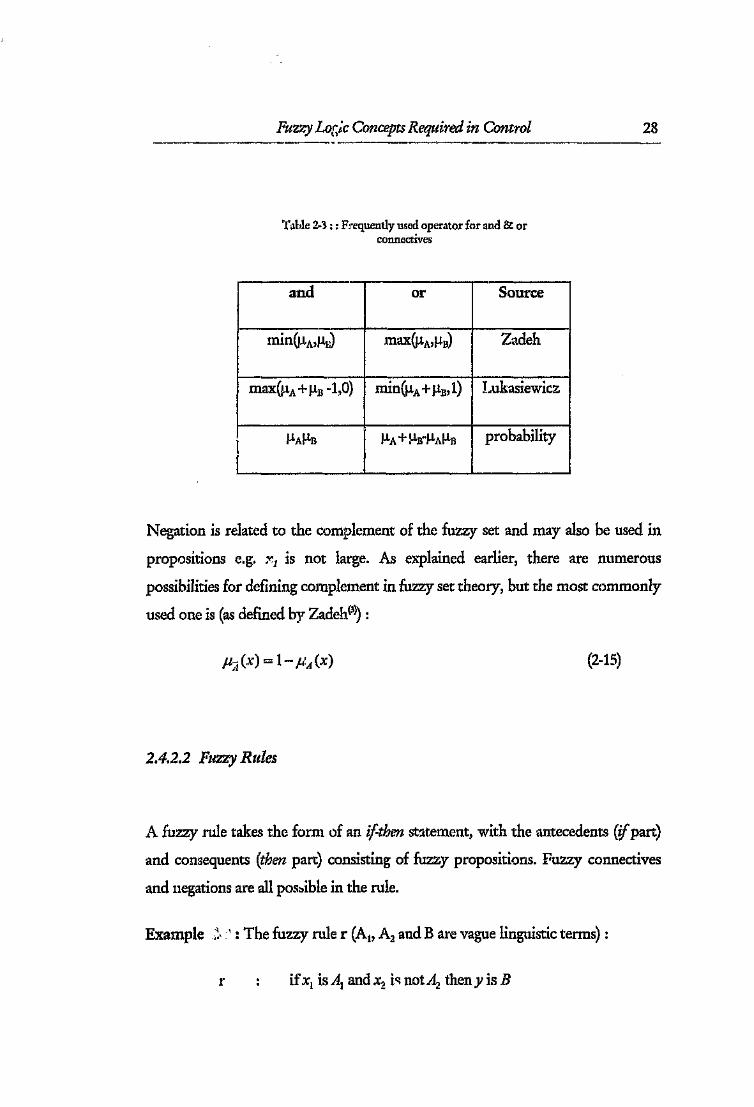
Table 2·-3 : : Frequently used operator for and & or connectives 28
Table 3..1 : Summary of some fuzzy application " 62
Table 5··1: Comparison between tiJ:~z;rand classical control design 114
Table At :Model parameters for servo motor " 128
Table A.2 : Model parameter values fer CSTR " 128
Table 1\.3: Model parameter values for tank system 131
Table C.l : FU7~:,;;iset symbols 146

XlV
List of Symbols
)
o
p(.)
T(·)
S(·)
1(·)
core(·)
hg~(')
supp(·)
x.t
R
CSTR
dB
FAM
set intersection/ conjunction
set union/ disjunction
sup-min composition
membership function
T-norm
T -conorm/S-norm
Inference
core of fuzzy set
height of fuzzy set
support of fuzzy set
ithnumerical input value
jth numerical measured input value
ithinput universe
fuzzy set for jtltinput universe
fuzzy set for illtinput universe in antecedent of kth rule
ktll fuzzy rule
fuzzy relation
jth numerical output
rh output universe
fuzzy set for r output universe
fuzzy set D'J1' r output universe resulting from inference
continuous stirred-tank reactor
decibels
fuzzy associative mcmol1'
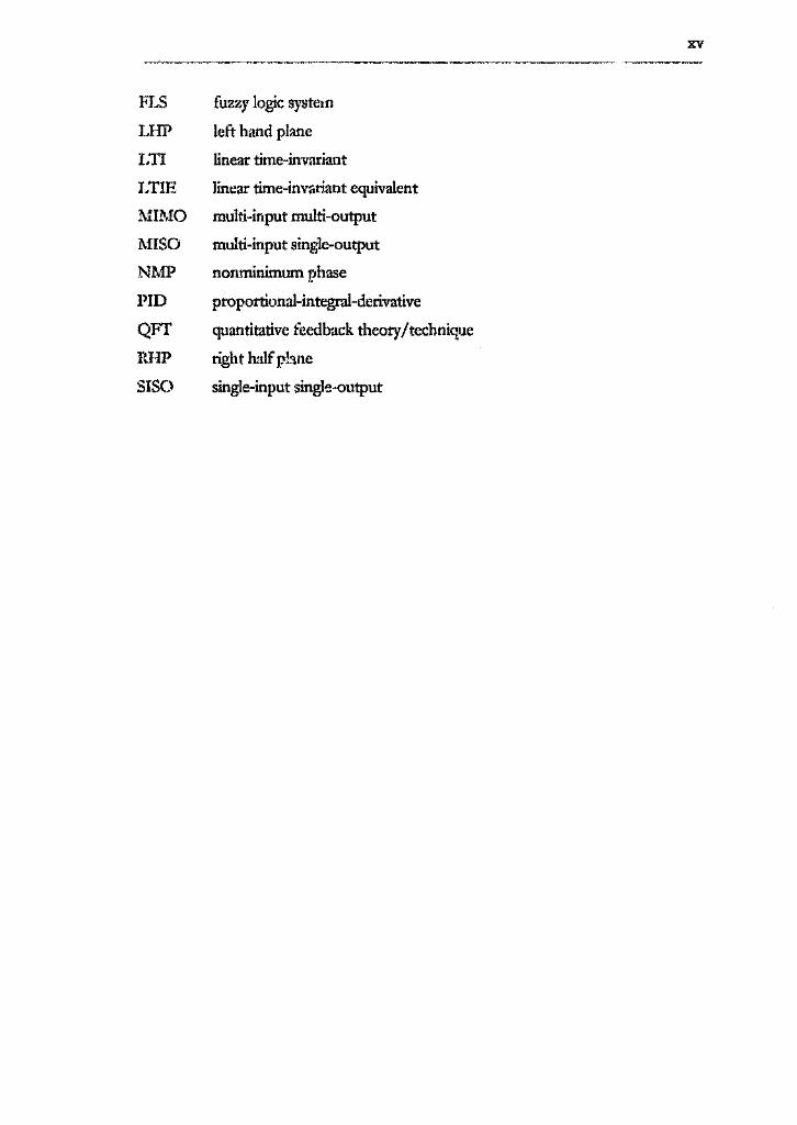
FLS
LHP
r.nLTIE
MI.MO
MISO
NMP
PID
QFfRBPSISO
fuzzy logic system
left hand plane
linear time-invariant
linear time-invariant equivalent
multi-input multi-output
multi-input single-output
nonminimurn phase
proportional-integral-derivative
quantitative feedback theory/technique
right half plane
single-input 'single-output
xv

Introduction 1
1. Introduction
Fuzzy logic has recently become a popular topic in various fields especially
controL Many journals, Internet 1iewsgroups' and books on the theory and
applications of fuzzy logic have bee, ime available, Despite an this, there is much
misunderstanding about the nature cf fuzzy logic and its limitations. The aim of
this project report is twofold, firstly to investigate what fuzzy control has to offer
and secondly to compare it to classici control.
1.1 What is fuzzy control :;>
When controlling a process, human operators encounter complex patterns of
process dynamic behaviour which are difficult to interpret and model. Lack of a
mathematical model leads to problems in classical control design. These complex
process behaviour patterns can often be reduced to a set of linguistic operating
rules which the operator uses to enforce control on the process. The rules
themselves include . .iprecise terms (hot, cold, fast, slow) which are multivalued,
Fuzzy set theory and the application, fuzzy control, offer a method of using this
imprecise multivalued information to control a process. Fuzzy set theory has
been used in the fields of linguiscics, psychology, economics, information
retrieval'" and the soft sciences (e.g. branching questionnaires'i'). Most problems
which are defined using vague terminology can use a form of fuzzy logic to model
the problem.
I The main newsgronp is camp" a.i . fuzzy.

Introduction 2
Fuzzy set theory deals with sets where the membership is a matter of degree and
not absolute, as is the case with classical set theory. Fuzzy set theory serves as the
basis for fuzzy logic', Fuzzy logic is a ru'e based means of inferring an action
(consequent) from an input (antecedent) using fuzzy sets. Fuzzy control is the
application of fuzzy logic to the control of a physical process.
The fuzzy controller, in particular, consists of a collection of user defined control
laws. These laws are fired in parallel. Each rule which is fired, contains a certain
truth value which determines the degree to which the rule conditions have been
met. The recommended cor+ol action is derived by combining the results of each
rule in a prescribed manner <isdescribed in Chapter 2. The fuzzy controller may
be defined as a non-linear mapping from the input space to the output space. The
term "fuzzy" comes from the vagueness in the linguistic terms which are used in
the statement of the rules, However, the fuzzy controller gives a precise meaning
to the vague linguistic terms.
1.2 Fuzzy control
The first paper on fuzzy control was written by Zadeh'", This paper and othersl4,5
et al) laid out the basic structure of the fuzzy controller. In 1974, Mam&mi(6)
proposed using fuzzy sets for the control of a physical process. Mamdani and
Assilian'" later reported on the application of fuzzy control to the control of the
steam pressure and throttle setting of a small laboratory engine. This was the first
practical use of fuzzy control and proved that it offered a viable control
methodology. Lemke and Kickert(8)then used fuzzy control for the control ,l a
warm water plant. Since then, fuzzy control has been formalised in the
literature(9,IO,ll,l2)which introduce the theory with suitable applications'l", The
-----.-----1The theoretic operations 011 fuzzy sets form the base for the logical operators.
Introduction 3
trend has been to apply fuzzy logic to as many applications as possible withou
examining what exactly is being achieved'" et al).
Fuzzy control is enjoying a large amount of "applications pull". This means that
the success of applications has led to the theory being formally developed and
problems being addressed. Fuzzy control books and papers(15)are being written
for people with little or no background in fuzzy logic or control. Thus the trend
is to ignore what lies below the "surface" and use fuzzy control without having an
understanding of the concepts. This results in a control design where the trade
offs and benefits are not fully u aderstood,
Fuzzy control is very widely used in commercial consumer products such as
video cameras, motor cal. washing machines and vacuum deaners(16). The
western countries have been slower to accept fuzzy control due to its lack of
mathematical tools, but the success of these applications has ensured that it is now
taken seriously. Another reason for the slow acceptance is psychological. It is felt
that instead of accepting the "fuzziness" of a system, the trend should rather be to
obtain a more accurate model.
1.3 Problems and myths surrounding fuzzy logic
The hype surrounding fuzzy control has resulted in numerous myths regarding
its use and benefits. Some of the claims made by fuzzy logic proponents are given
below:
1. Fuzzy controllers are easy to understand and design. The skill level required
to design a fuzzy control system is less than that required for a classical
controller(15,17,18). Therefore personnel and training costs are reduced.
2. Fuzzy controllers are more robust than classical controllers'l",
Introduction 4-----~--~--.-----
3. Fuzzy control is more suited to non-linear processes(iOctal).
4. Development time of fuzzy controllers is less than that of classical
controlIers(15,17).
5. Fuzzy control improves performance'" et al).
6. Fuzzy control reduces hardware costS(17).
There are also numerous qualitative benefits claimed about productivity which
will not be addressed here.
Claim (1) is true to a certain degree. The high level programming of fuzzy control
systems is easy to understand and requires less control knowledge than required
by a classical control system designer. This comes at a cost however. After
designing the fuzzy controller, the c:uality of control is based solely on the
correctness of the rules and the quality of the underlying fuzzy controller. The
assumptions made by the fuzzy control designer must be appropriate to the
system being controlled, so that the operator rules used by the controller are
appropriate. To design a controller and take into account all the factors required
by a classical control designer, the required knowledge about the controlled
system is the same for both approaches. If it is not, then assumptions are made
about the system which may not be valid.
Claim (2) concerning robustness is more complex. Typical investigations'i" claim
that their fuzzy logic controller is robust if it works when rules are either
removed or tampered with. This is not a very practical definition of robustness as
fuzzy controllers do not generally simply lose rules. In this investigation, the
classical definition of robustness is used. This involves the controller's ability to
deal with parameter variations, noise, unmodelled dynamic system characteristics
and disturbances. Whether the fuzzy controller is more robust than a classical
controller depends 011 the rules and sets defining the fuzzy system, as will be
shown in Chapter 5. A fuzzy system can model any linear system to an arbitrary

Introduction 5
degree, so Claim (2) should be altered to the fact that a fuzzy system can be as ( or
more ) robust than a classical system. The level of robustness depends 011 the
designer. The root of the problem is that at present it is difficult to quantify the
robustness in the fuzzy control domain.
Claim (3) regards the suitability of fuzzy control to a non-linear process. The
fuzzy controller is a non-linear control method, so it is obvious that it has the
capability of controlling a non-linear process better than a linear controller I -n,
The situation, as is discussed in Chapters 5 and 6, is not always about the level of
non-linearity of the plant, but also about the level of information about the plant.
Simply because a system is non-linear does not mean that a fuzzy controller will
easily be able to control the system. Significant qualitative knowledge is required
about the dynamics of the plant. The situation is further confused by claims(:!1)
that fuzzy systems offer better response on a linear system as well. This claim is
also investigated in Chapter 5.
Claim (4) : The development time of fuzzy controllers is dependant on the
control problem and designer, thus Claim (4) is a gross generalisation and cannot
be seen as a benefit. The development time is a function of the amount of
information available, the type of information, the complexity of the problem
and numerous other factors. This also defeats Claim (1).
Claim (5) : Fuzzy logic control, through its non-linear nature, has the ability to
provide better performance than a linear controller. The problem is in knowing
what the right choices' are for the fuzzy controller which will give the superior
control, as the methodology is not transparent with regard to these choices.
Claim (6) : With the recent speed of technological development, fuzzy chips are
becoming more freely available at low prices. Thus a dedicated fuzzy chip is much
1 The rules, membership functions, conjunctions and implication method need to be defined in any fuzzycontrol system.

Introduction 6
cheaper than a similar DSP board, which would be required if the application
requires complex control actions. However, conventional PID controllers still
offer the cheapest and easiest control.
The main problem regarding fuzzy control is the lack of transparent design and
analysis tools. The current methods of controller design and verification are
simulation and complex, but limited mathematics. The design procedure is
typically iterative with stability, robustness and other aspects being investigated
through simulation. This is in contrast to the well developed transparent design
and analysis tools for classical control design(n).
1.4 The aim of this investigation
Section 1.3 highlighted the uncertainty and problems regarding fuzzy control
design and analysis, The aim of this investigation is to :
• define the position which fuzzy control should hold given its current level of
development. This includes where fuzzy control should be used and where it
could be used if some problems are overcome.
• define the areas of fuzzy control which require more investigation and thus
require more research.
e qualitatively and quantitatively compare fuzzy control to classical control.
• investigate how fuzzy control deals with pertinent issues present in control
theory.
Prior research around this topic(23,24)has restricted itself to issues regarding the
suitability of fuzzy control to certain areas in the control domain. These papers
look at past applications and from these determine the areas best suited to fuzzy

Introduction 7
control. The aim of these papers has been to define where and when to use fuzzy
control on a broad scale. What is lacking is a controller comparison using specific
control issues. Noise rejection and other issues are glossed over. This investigation
will deal in particular with robust control and issues pertinent in classical control
theory (usually dealt with superficially if at all), such as stability, disturbance
rejection, noise suppression and parameter variation. Dead time and non-
minimum phase plants are also investigated. At all mes the investigation is
intended to be fair and the information used in the control design is noted. It is
essential that the most appropriate information be made available to both the
fuzzy and classical controllers for the investigation to be fair. Where the
information is different this is noted.
The investigation is performed through two means:
• A literature survey of past applications, with emphasis on the problems fuzzy
control has been successfully applied to and the benefits which were achieved.
• Using numerous computer based models wherein particular control aspects
about fuzzy control are investigated,
This investigation showed that:
• The area where fuzzy control should be used is not obvious or easily defined.
The particular circumstances surrounding the control problem determine
when fuzzy control is more appropriate.
• Various aspects regarding fuzzy control need to be addressed. These include
mathematical design and analysis tools as well as developing a clear
understanding of the implications of certain design choices.
• The non-linear nature of fuzzy control as well as the ability to include
qualitative information are major advantages over clossical control.

Introduction 8
• Methods ')f including certain control aspects (e.g. parameter variation, noise
suppression) into the fuzzy design process is not clearly defined.
1.5 Approach taken
The investigation) as outlined in section 1.4, is conducted in the following way:
Chapter 2 introduces the essential theory required for the design and analysis of
fuzzy controllers. It introduces only the theory rel zvant for this study as well as
an overview of the types of fuzzy controllers available. Chapter 3 contains a
literature survey of the current applications in fuzzy control, a discussion of the
relevant control aspects and the approach taken in the investigation. These two
chapters are essential for the rest of the investigation to be put into perspective.
The modelling of the computer based plants is given in Chapter 4. Chapter 5 is a
summary of the designed controllers and a comparison of results. These results
include design and implementation issues as well as the final simulation results.
Conclusions based on these results are given Chapter 6.
AU simulations were performed on Simulink under MATLAB~ Version 4.2. The
fuzzy logic toolbox was used to implement the fuzzy controllers. The QFT
designs were developed with the aid of the MATIAB" QFT toolbox. All significant
code and the Simnlink models are given in the appendices.

Fuzzy Logic Concepts Required in Control 9
2. Fuzzy logic concepts required in
control
This chapter contains an introduction to the fuzzy set and fuzzy logic theory
which is required to generate a fuzzy logic controller. The content deals only
with the concepts relevant to fuzzy logic as applied to the control field, and thus,
is not a comprehensive guide to fuzzy systems. This section is derived from a
number of sources (particularly Jager{lO),Mendelv'', Jang(15)and Kosko(12)),and for a
more detailed approach to fuzzy logic, the reader is referred to them. There is a
large resource of literature which reviews the required theory in more detail.
Firstly, the fuzzy system is defined and explained. Fuzzy set theory is then
introduced followed by the principles of fuzzy logic controller design. The
structure and principle of the fuzzy controller is also dealt with. The fuzzy logic
system as a universal approximaror is also discussed. Finally the concepts behind
adaptive fuzzy control are introduced.
2.1 Definition of a Fuzzy Logic System
The term fuzzy is derived from the fact that membership to a set (e.g. tall people)is not crisp, but graded (e.g. 20% membership to the set tall). Thus the set "tall" is
a 'fuzzy' concept with people of various heights being members to various
degrees. Classical set theory calls for a bivalent' approach where membership is
either true or false. Fuzzy set theory allows multivalence and hence various
degrees of membership are possible'i".

Fuzzy Logic ConceptsRequired tn Control 10
A fuzzy logic system is a non-linear mapping of an input vector into an output
vector. Fuzzy controllers are represented by iJ-then rules and can thus provide a
user-friendly method of interfaci. ,~with the controller. The rules are fired" in
parallel (or in an arbitrary order when programmed'), each to a certain degree".
The result of all che rules are aggregated to a final crisp value which forms the
output of the fuzzy systems. The rules deal with linguistic variables which are
defined (through membership functions) in the universe of discourse (see section
2.3 for definitions).
:'uzzy sets have come under a 10i: of criticism for being "probability in disguise".
It is the author's opinion that this is not true. There is a similarity in the way it is
termed, but the meaning is different. Probability still remains based on a bivalent
system, where membership is definite. Fuzzy membership is multivalent and
therefore membership is definite, but to varying degrees. For example, a 1.5 metre
man could be seen as belonging 60% to the set "tall" and 40% to the set "not tall".
To say that he has 60 % chance of being "tall" means that he is either tall or he is
not, but he has more chance of being tall. The man cannot be a member of "tall"
and "ncr tall" as is the case with fuzzy logic.
2.2 Rationale for Fuzzy Logic
The rationale used to justify the study of fuzzy logic in engineering is given by
Lofti Zadeh (Principle of Incompatibility) (4) : "As the complexity of a system
t By bivalence, it is meant that the set membership can only take on two values, namely true (1) or false (0).
2 By fired, it is meant that the rule antecedent is met. Ina fuzzy sense, the rule antecedent is always met, butoften this is to a zero degree, as the required membership is zero.
1The actual order is not important as the results are aggregated afterwards.
1The degree to which the rule is fired depends on the applicability of the antecedent. II the membership of thefuzzy set called ill the antecedent is low, the degree of firing is low.
S This need uot be true, but is true for a fuzzy controller.

Ft!zzy Logic Concepts Required in Control 11
increases, our ability to make precise and yet significant statements about its
behaviour diminishes until a threshold is reached beyond which precision and
significance (or relevance) become almost mutually exclusive characteristics." The
ability to allow for a less precise definition of certain properties which are being
controlled or analysed, allows a method of incorporating real-world "fuzziness"
or uncertainty into a designed controller.
2.3 Fuzzy Set Theory
2.3.1 Fuzzy Sets
Zadeh'" (1965) introduced fuzzy set theory in his paper "Fuzzy Sets", but others
such as Lukasiewicz ( who introduced multivalued logic) and Max Black(26) ( who
c....lled it vagueness) had introduced the ideas earlier.
A ..zy set (A) is a set with graded membership defined ever a universe of
discourse and is characterised by a membership function PA(x) E [0,1]. The
universe of discourse is the input space for a specific fuzzy system input. A fuzzy
set A, in the universe of discourse X, is denoted by:
A :=: ~ l[l(X) / x..At J'" ~ I I;,,1
== Jl,t(X1) / XI+· ..+J~I(X'.'I) / >'~/I
(2-1)
for a discrete X. Thus for each value of x on the universe of discourse X, PA(x)defines the membership of x to the set A. The summation sign does not denote
actual summation, but rather the collection of the discrete points. Similarly, the
forward slash does not denote division, but rather the association of the fuzzy set
membership values with the input ~:pace.
Fuzzy Logic Concepts Required in Control 12
For a non-finite (continuous) X, the equation can be written as :
(2-2)
where the integral sign does not ek .ute integration, but rather the continuous
collection of defined points.
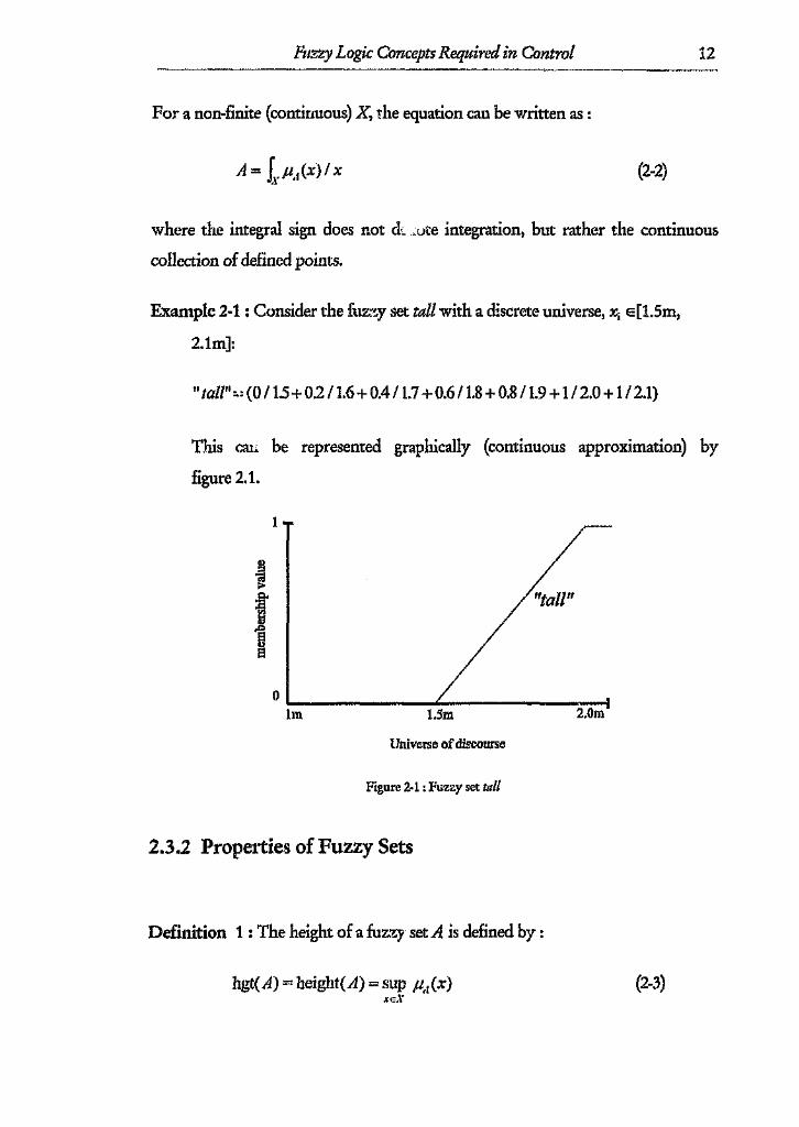
Example 2-1 : Consider the fl1Z:3Y set tall with a discrete universe, Xi E[1..5m,
2.1m]:
"tali:» (0/1.5 +0,2 / 1.6+ 0.4 / 1.7+ 0.6 /1.8 +0.8 / 1.9+ 1/ 2.0 +1/2.1)
This cai; be represented graphically (continuous approximation) by
figure 2.1.
~------------~-------------~2.0m105m
Universe of discourse
Figure 2·1 : Fuzzy set tall
2.3.2 Properties of Fuzzy Sets
Definition 1: The height of a fuzzy set A is defined by :
hgt(A) == height(A) = sup p,j(x)X"X
(2-3)

Fuzzy Logic Concepts Required in Control 13
A normal set IS one which has a height of 1. Any h!ZZY set can be converted into a
normal set through division by the supremum of the set. The height corresponds
to the maximum membership that the set allows.
Definition 2; The core of the set is the part of the set for which the membership
IS unity :
core(A):::: {x E Xllt,l = I} (2-4)
This is the range on the universe of discourse for which a fuzzy set gives complete
membership.
Definition 3.: The support of the set, is the part of the set for which the
membership is greater than () :
supp(A):: {x EXIJlA(X) >O} (2-5)
If the support of ~ set is a single point, the set is known as a fuzzy singleton.
Definition 4: The acut of a fuzzy set (also termed level set) is defined by :
(2-6)
The point where the membership is 0.5 is termed the crossouer point.
There are more properties of fuzzy sets which are not discussed here as they are
not necessary for the design of controllers.

Fuzzy Logic Concepts Required in Control 14
2.3.3 Linguistic Variables
Zadeh(27)explains the linguistic variable in the following way: "In retreating from
precision in the face of overpowering complexity, it is natural to explore the use
of what mighz be called linguistic variables, that is, variables whose values are not
numbers but words or sentences in a natural or artificial language", His rationale
for using these variables is expressed by : "The motivation of the use of words or
sentences rather than numbers is that linguistic characterisations are, in general,
less specific than numerical ones."
Let tt denote the name of a linguistic variable' (e.g, height) with numerical values
denoted by x, where XEx' The linguistic variable is usually decomposed into a set
of terms, T(1/.), which cover the universe of discourse. These terms can bp-characterised as fuzzy sets with membership functions,
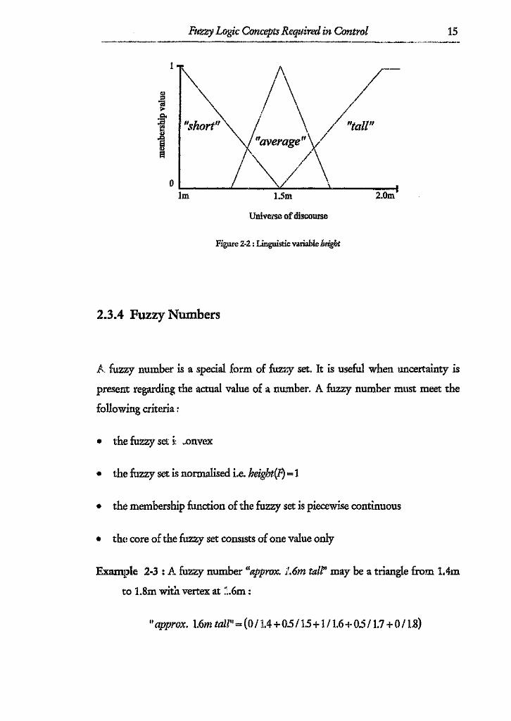
Example 2-2: If height(x) is a linguistic variable, then it can be decomposed into
the following T(heigbt) =.{short, average, tall} where the universe of discourse
could span X=[lm, 2.1m]. Each term is characterised by a membership
function 'adicating the degree of membership for any value of x within the
universe of discourse X. Following on example 2-1, the following terms
(which form the linguistic variable), can be defined:
1 Sometimes x and II arc used interchangeably, especially when the linguistic variable is a letter.
Fuzzy Logic Concepts Required in Control 15
15m
Universe of discourse
Figure 2-2 : Linguistic variable height
2.3.4 Fuzzy Numbers
A fuzzy number is a special form of fuzzy set. It is useful when uncertainty is
present regarding the actual value of a number. A fuzzy number must meet the
following criteria:
• the fuzzy set i .onvex
• the fuzzy set is normalised i.e. height(F) = 1
• the membership function of the fuzzy set is piecewise continuous
• the: core of the fuzzy set consists of one value only
Example 2-3: A fuzzy number "approx. /.6m tall" may be a triangle from 104m
to 1.8m with vertex at :~.6m:
"upprox. 1.6m tall":.::;(0 /1.4 + 0.5/1.5 + 1/ 1.6+ 05 /1.7 + 0 /1,8)

Fuzzy Logic Concepts Required in Control 16
A fuzzy interval must meet the same conditions for a fuzzy number but the core
is not restricted to one number {e.g. "from about 1.2m to about 104m tall").
Operations can be performed on fuzzy numbers (e.g. addition, subtraction etc.)
using the extension principle'",
2.3.5 Membership Functions
A membership function is a curve defining the degree of membership for each
point on the universe of discourse. The membership must be between 0 and 1, but
does not necessarily have to include 0 and 1. The shape of the membership
function can be arbitrarily set, based on the designer's discretion, or, as is
currently the trend, the shape can be designed through optimisation procedures
(like neural networks(l.O,15)).
Example 2M4: The linguistic variable height contains the membership function
for tall. The definition of tall people is not a universal one, and hence the
shape will vary depending on the designer's perception of tall people. An
infinite number of possibilities can be designed and it is objectively
impossible to say which designer is most correct in his interpretation of tall.
The !~reater the number of membership functions (hence fuzzy sets) on the
universe of discourse, the greater the resolution that can be achieved. The higher
the density of the fuzzy sets on a certain part of the universe of discourse, the
more complex the controller output as a function of the controller input can be
defined(lD).

Fuzzy Logic Concepts Required in Control 17
Table 2-1 is a summary of the most common membership function shapes,
Table 2-1: Summary of common membershipfunctions
t-s_h_a_p_e t--E_qU_a_t_io_n__ :- -"-----~
I~_-~'Xa' : ax<bb-a'-'-
fix.a.b.c) =.:1c-x-- b< <b ' s x s.cc-
o,c~x
Triangular
Gaussian -(.t-ct:.f(x;cr,c)::: e 2(1"
Bell Curvef(x;a,b,c) = I" 1211
1 x-c+~-a
Trapezoidal /'(x,a,b,c,d) :::
O,x:::S;ax-a-b-,a:::s;xsb-a
l,b :::;;x:::S;cd-x--- c<x<dd-c"- -
O,d:::S;x

Fuzzy Logic Concepts Required in Control 18
2.3.6 Operations 011 Fuzzy Sets
As with crisp sets, intersection, union and complement are defined in fuzzy set
theory, but as the membership values are no longer restricted to {O,l}, but rather
the interval [0,1], the operators are not uniquely defined.
2.3.6.1 Union and Intersection
Let fuzzy sets A and B have membership functions J.tA and J..LB respectively. Zadeh{3}
defined the following:
PAnll := min(,uA(x),,uJ;(x» (intersection)
,uAvii = max(PA (X),,uIJ(x) (union)(2-7)
IfA and B are crisp sets, the definitions agree with the crisp set definitions. This is
because the intersection and union criteria (discussed below) which must be met
are the charar =ristic functions found in crisp set theory. The following
definitions have also been proposed' :
,uAnll = J.lA(X)~II(x)PAvll := pAx) + ,uIJ(x) - pAx)PIJ(x)
(intersection)
(union)(2-8)
There are, however, an infinite number of algorithms which implement fuzzy
intersection and union. Thus the general forms, T-norm (triangular norm) and T-
conorm or S-norms (triangular conorms) are used respectively.
The Tsiorm (intersection) is a two place function T : [0,1] x [0,1] --)0 [0,1] which
satisfies:
• boundary: T(O,a) =T(a,O) =0, T(a,l) =T(l,a) =a
I Based on the definitions from probability,

Fuzzy Logic Concepts Required in Control 19
• monoronicity : T(a.b) ~ T(c,d) if a ~ c and b ~ d
• commutativity: T(a,b) =T(b,a)
• associativity: T(a, T(b,c) )=T( T(a,b) ,c)
Many symbols are used for the T-Ilorm, but the most popular IS *. The
convention used from this point on will be a capital T.
The rules for T-eonorm are similar. The T-conorm or Snorm (union) is a two
place function S : [0,1] x [0,1] -~ [0,1] which satisfies:
• boundary: S(O,a)=S(a,O)=:i,S(a,1)=S(l,a) =1
• monotonicity : S(a,b) ~ S(c,d) if a ~ c and b ~ d
• commutativity: S(a,b)=S(b,a)
• associativity: Sea,S(b,c) )=S( S(a,b) ,e)
The fuzzy system designers can therefore design their own T-norms and S-norms
should it be necessary. All T-norms and 'I'conorms will produce the same results
when used with crisp set theory, but different results with fuzzy set theory.
Example 2-5: Table 2-2 shows the results of different T-norms and T-conorms.

Fuzzy Logic Concepts Required in Control 20
Table 2-2 : Effect of choosing different connectives
T-norm Tconorm
Zadeh: max(!-LMlln)
\
\
Lukasiewicz:
max(!-LA + lln-l,O)
Lukasiewicz:
I
/\
\I
/
I
/ \
\
Fuzzy Logic Concepts Required in Control 21-~- ---,------
2.3.6.2 Complement
Zadeh(3) proposed the following membership function for fuzzy complement:
(2-9)
This definition is again, not unique. The requirements for the complement of a
fuzzy set A are:
• c(O)= 1
• c(a)<c(b), if a > b
• c(c(a)) = a
There are other definitions of fuzzy complement which meet the above
requirements including the A-complement according to Sugenv(28}.
From the above definitions, it can be seen that for fuzzy sets, the crisp set Laws of
Contradiction (A uA =: U) and Excluded Middle (A nA :::::tft) are broken. The
implication of this is that it challenges the basis of Aristotlian binary logic. A cup
can be both half fun and half empty (or not half full) with fuzzv SAt theory, where
crisp theory requires that it be either full or empty.

Fuzzy Logic Concepts Required in Control 22
2.3.7 Fuzzy Relations and Compositions
2.3.7.1 Fuzzy Relations
The fuzzy sets discussed before have only had membership functic of one
variable. They can be extended to more than one variable and are then termed
fuzzy relations. The fuzzy relation represents a degree of presence or absence of
association, interaction or interconnectedness between the dements of two or
more fuzzy sets(ll).Given the fuzzy relation R :Xjx .. ,xX" -4 [0,1] then
(2-10)
Example 2·6: The fuzzy relation for approximately equal R/;..igl;V:-(X, y), can be
described by:
R'Jeigl;t,,(X, y)= 1/(1,1) + 0.5/(1,1.1) + 0.5/(1.1,1) + 1/(1.1,1.1)
+ 0.5/(1.1,1.2) + 0.5/(1.2,1.1) + 1/(1.2,1.2)
+ ... + 0.5/(2.4,2.5) + 0.5/(2.5,2.4) + 1/(2.5,2.5)
for the space X=[lm,2.5m] & Y=[1m,2.Sm]. This relation gives an
indication of whether two people's heights, x and y, can be considered equal
or not. For example if one person is 2m tall and the other is 2.1m, we can
say that they are approximately equal to degree 0.5.

Fuzzy Logic Concepts Required in Control 23
oa
2~ " . - .;-.- _-.~.,_.
, 1
Figure 2·3 : Fuzzy relation RbcizbL"'(X, y)
2.3.7.2 Fuzzy Compositions
Composition involves taking two relations from different product spaces and
combining them to form another relation which relates the elements of the new
pro+ret space. For the general case', the composition is denoted by :
R(U,W) = P(U,V) 0 Q(l ,W) (2-11)
where 0 is the composition operator.
The fuzzy composition is defined by Zadeh'", "suppose there exists a fuzzyrelation R in X x Y and A is a fuzzy set in...~ then a fuzzy subse, ;; of Y can be
induced by A, given the composition of RandA". This is denoted by
B=AoR
1For both crisp and fuzzy set theory.

Fuzzy Logic Concepts Required in Control 24
Therefore if a relation R relating B and A is known, the given A (or B), B (or A)
can be inferred. The sup-min composition, proposed by Zadeh, leads to the
following implementation. IfA is a fuzzy set with membership function Il'l('\,) and
R is a fuzzy relation with membership function f.l/ ;,y) :
f.luCv):;-" sup min(f.l.l(x),f.l/l(x,y))xcX
(2-13)
A generalisation of (2~12) using T-norms and Tconorms is :
(2-14)
Composition is the procedure that allows a fuzzy model to produce sensible
outputs for previously unseen inputs, provided the fuzzy rule base and input sets
are appropriate.
Example 2-7: (adapted from Jager(lO})Following on example 2-6, where Rhcigbt",(X,
y) is defined, and example 2~3,where A"''!.6m is defined, below is a discrete
composition.

Fuzzy Logic Ccncepts Required in Control 25--~~ ..~......------------. ~._,..--_._- ..~--.- ..--
Jlheight ", (x,y)p"u,,.(s)I""""'~ ,,--- ---"--------..,(0 0 0 0 0 0 o 0 0 0 0 0.5
() I) o 0 0 o o () 0 () 0.5 I ('5() 0 0 () (J n 0 u (J U.S I 05 e() 0 0 0 0 (j 0 0 (;.5 I 0.5 0 [)
0 0 0 o 0 0 0 05 0.5 0 0 II IJ.llJ(Y) ==
05 0 0 0 0 0 OJ I 0.5 () 0 I) ~II (j 0 II 0 0.5 0.5 (J (J o 00.5 0 0 0 0.5 1 05 0 0 0 0 0 :j0 0 0 05 1 0.5 G 0 o 0 0 00 o 0.5 o.s (I 0 0 () " () 0
0 05 0.5 o IJ 0 0 0 0 () 0 n0 1 O.S o 0 () 0 0 {J () 0 0 ()
lilin(t1 (X,I, tl, . I (x, y»)::,;: .wlg:t ~-A--- ..___ ._~
r~0 0 0 0 0 0 0 0 0 o
11I) 0 !l 0 0 0 0 () 0 00 0 0 o () 0 o 0 0 0 0
010 0 (l 0 0 0 0 0 U D o(l 0 () 0 0 0 (J 0 0 0 0 0
=10(J 0 () () 0.5 o.s 0.5 0 I) 0 ()
() 0 0 0 05 I OJ 0 0 0 0 0
10 0 () o.s 0.5 ~.5 0 (I () 0 () 0
I~0 () () (I 0 0 0 0 0 0 ~jo 0 o 0 ~) 0 () 0 0 0
l~0 () () o 0 0 () 0 0 () ()
() () 0 0 (\ 0 0 0 0 0 0
Max Min(/ld,.,Tn (.~),II"(»,y))x
"--
::: (0 0 0 0.5 0.5 I 0.5 as () () 0 0)

Fuzzy Logic Concepts Required in Control
2.4 Fuzzy Logic Systems
-, ...._._.,_.---- -.~.-.-- ----1I
Ii
S'=A'oR
c;o~t;:::
Fuzzy oNOutput NSets 'W
o
Figure 2-4: Elements of a fuzzy logic system
26
IIII.I
The structure of the most widely used fuzzy controllers is depicted in Figure 2-4.
It consists of four major components, namely the rules, fuzzifier, inference engine
and defuzzifier. Once the controller has been designed, the fuzzy system maps a
crisp value on the input into a crisp value on the output i.e. Y= f~'C), where f is
some (usually non-linear) function.
Note: From this point forth, any symbol with a "dash" represents a measured
variable (or derived from measurement). E.g, x' represents a measured
value on the universe of discourse of X.
....
Fuzzy Logic Concepts Required in Control 27
2.4.1 Input Fuzzification
The fuzzification stage of the fuzzy controller involves the construction of the
fuzzy input relation. Fuzzification is not always necessary if the input is already a
fuzzy relation. If the input to the controller is a numerical value (most common
case), then the fuzzy input set A/ is given by the singleton,
{I, if Xi = x:
, x.)=flA; ( 1 0, otherwise
Some sources(15)include the matching of fuzzy propositions into the fuzzificarion
stage.
2.4.2 The Rules
2.4.2.1 Fuzzy Propositions
A fuzzy proposition is a statement such as "x is large", where in this case "large" is
a linguistic term referring to some fuzzy set on the universe of discourse of
variable ,x,Logical connectives (and& or) are implemented using the Tsnorms and
'I'conorms.
The most common connectives which are used are summarised in Table 2-3 :
Fuzzy LorJc Concepts Required in Control 28
Table 2-3 ; ; Frequently used operator for and & orconnectives
and or Source
rnin(llA,!ln) max(!lAll-ln) Zadeh
Imax(p'A+J..Ln -1,0) min{IlA+ J..LB,l) Lukasiewicz
~LA!lB L~B-~AI-lBprobability
INegation is related to the complement of the fuzzy set and may also be used in
propositions e.g. 71 is not large. As explained earlier, there are numerous
possibilities for defining complement in fuzzy set theory, but the most commonly
used one is (as defined by Zadeh(3)):
(2-15)
2.4.2.2 Fuzzy Rules
A fuzzy rule takes the form of an if then statement, with the antecedents (if part)and consequents (then part) consisting of fuzzy propositions. Fuzzy connectives
and negations are all possible in the rule.
Example ;~.' : The fuzzy rule r (Al' A2 and B are vague linguistic terms) :

fifZZY Logic Concepts Required in Control 29
can be written as,
where I is a fuzzy implication function (see section 2.4.3.1) and T IS a
conjunction based on the Tsnorm.
2.4.3 Fuzzy Inference Scheme
Note : The fuzzy system discussed here uses local inference' as it is more
commonly used in fuzzy control applications'f'.
2.4.3.1 Inference of a single rule
The inference of a single rule is the application of the composition of fuzzy
relations. The compositional rule of inference was introduced by Zadeh(4). It
assumes that a fuzzy rule
if x isA then y is B
is represented by a fuzzy relation R. The result B I can then be inferred through
the composition of A Iand R :
B'= A'oR (2-16)
I Local inference (rule-based approach) means that each rule is inferred and the results of the inferences of theindividual rules are aggregated afterwards. Global inference (relation based approach) means that the rulesarc aggregated and used for inference as a whole, This makes no difference if the inference with T-implications is used or the inputs arc numerical.
Fuzzy Logic Concepts Required in Control 30
Like the other operators in fuzzy set theory, the number of possible implication
methods is Infinite. The implication method chosen for control is typically the T-
implication (based on the T-norm).
I(a,b) = T(a,b) (2-17)
This complies with the classical implication as expected.
2.4.3.2 Inference of (.1 rule base
The fuzzy rule base consists of rules of the form,
r1 if Xl is Au and .. , and xN)S AN.\" ,1 then y is B,
else
else
rk if Xl is At,k and ... and XN\ is AN.\".k then y is B,
else
else
I:"lr if'x, isAI,Nr and ... andxN_)sANr.Nr thenyis BN•
where N, is the number of parallel rules which have an antecedent based on N;
variables.
The fuzzy inference procedure can be divided into the following sections,
1. The numerical values obtained from the sensors (input to the controller) need
to be matched against the fuzzy rules. Thus, the numerical data x/, is matched
against the fuzzy propositions "Xi is Aj,k" in the antecedents of the fuzzy rules

Fuzzy Logic Concepts Required in Control 31
(2-18)
where 0\1: is a numerical value indicating the extent of the matching.
If the controller input contains uncertainty or inaccuracy, the input can be
modelled as a fuzzy number, and not a crisp number. In this case, the extent
of matching is:
(2-19)
where Ai I is the fuzzy number and hgt is the height of the fuzzy set.
2. Most rules will have more than one proposition, and therefore it is necessary
to determine the overall degree of fulfilment iJk (DOF) for each rule in the rule
base. A different method for each connective (and & or) is needed.
"'.\'
AND : fJk = Ta;,k (2-20a)i~1
NxOR : fJk = S«, (2-20b)
;'=1
Often rules may have both connectives. If this is the case, a combination of
the two methods is required.
3. The degree of fulfilment for each rule has now been determined. Thus, the
implication can be merle,
where I is the implication method used. The most commonly used method of
inference in fuzzy control is the inference with Tsimplications (based on the
Tsnorm) :

Fuzzy Logic Concepts Required in Control 32
(2-22)
The result is that each consequent Bk is restricted by the f3k value by means of
the 'I-norm, which represents the implication. Therefore, the rule is only
fired to the degree that its antecedents are fulfilled.
4. After the third step, the result is N, fuzzy output sets defined by the
membership functions JiBk' The sets must be aggregated to achieve a final,
single fuzzy set. There are (l"'ferent aggregation methods depending on the
method of implication. The method used when using the T-implication is :
(2-23)
where u is the union operator (or). If the max 'I'conorm is used, it results in a
final fuzzy set which is the maximum of all the individual fuzzy resultant sets.
Another popular method of aggregation is the summing method, where the
individual sets are added together.
Weighting of rules is also possible. If every rule is given a weight wkE[O,l], it
becomes possible to ensure that some rules have more influence in the
inference process. This is useful when a form of learning is being
implemented.
If the max-min inference method is used' (most common method), then the
process can be summarised by :
ropgrcgation
f.ill'(Y) =: ~ min (Ak,Jin (y))k ........__. kimplication
(2-24a)
where,
IMax-prod and sum-prod arc also fairly common.
Fuzzy Logic Concepts Required in Control 33
composition,----~projection,-'--1
ai,k == SUp m!!3 (P.1/(X;),/-iA"k(X;)combination
(2-24b)
conjunction,...-A-,
min ai,ki
(2-24c)
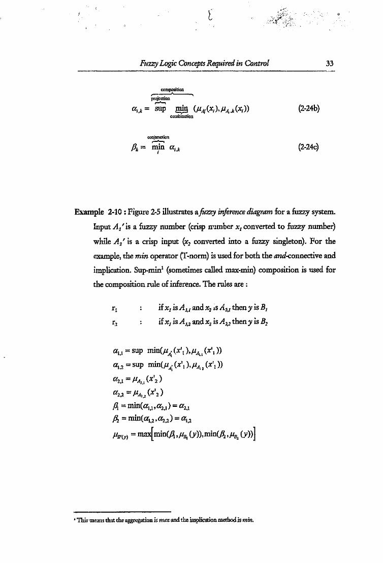
Example 2·10: Figure 2-5 illustrates afilzzy inference diagram for a fuzzy system.
Input At' is a fuzzy number (crisp number Xl converted to fuzzy number)
while A2' is a crisp input (X2 converted into a fuzzy singleton). For the
example, the min operator (f-norm) is used for both the and-connective and
implication. Sup-min' (sometimes called max-min) composition is used for
the composition rule of inference. The rules are :
if x, is AI,1 and X2 is A2,1 then y is BJ
if x, is A1,2 and X2 isA},2 then y is B2
a],l = sup min(PA; (x', ),PAI.I (x', »al•2 = sup min(PA; (x', ),PA.2 (x'!))
a2,1 ::;: PAz,1 (X'2 )
a2,2 == JiAl, (X'2)
f:lt =mineal,l ,a2,1) == a2,1
~ == min(a1,2,a2.2) = a1,2
f-ln'(y) = max[min(A ,PBI (y»,min(~ ,f-llJz (y»]
, TIllS means that the aggregation is max and the implication method is min.

,1_
Fuzzy Logic Concepts Required in Control 34
.,
Figure 2·5: Fuzzy inference diagram for example 2-10

Fuzzy Logic Concepts Required in Control 35
2.4.4 Defuzzification
The defuzzification st<lgetranslates the final fuzzy 5~ obtained after aggregation
into a numerical crisp value which forms the output of the fuzzy controller. The
method of defuzzification is not unique or bound by ,".f <Y ~pecific criterion. In
control applications, however, computational simplicity is desirable. Below is a
summary of the most popular methods of defuzzification :
2.4.4.1 Maximum Defuzzifier
This defuzzfier takes the maximum of the output set B' as its final output value.
This is not a good method as it ignores the set support distribution.
2.4.4.2 Mean ofMaxima Defuzzifier
As the name implies, this method determines the values of y where a maximum
in B 'occurs and computes the mean of these y values.
2.4.4.3 Centroid or Centre-of-Graoity Defuzzifier
This method is based on the principle used to calculate the centre of gravity of a
mass, except that the point masses are replaced by the membership function. In a

"FuzzyLogic Concepts Required in Control 36
one dimensional fuzzy set, this is often called the centre-of-area defuzzification.
The centre of gravity (COG) defuzzification method is defined by :
_ l,ulJ'(Y)'Y dyy=-.----
Jy fill' (y) dy(2-25)
and the discrete form is
(2-26)
where Nq is the number of quantizations in ..he membership function J1c. This is
the most popular method, but is, however, not computationally efficient.
2.4.4.4 Singletons
While not a defuzzification method, having singletons on the output simplifies
the defuzzification process significantly. These systems are often termed Sugeno-
style fuzzy systems after their developer'I", The consequent of the rules in this
system are crisp values (or singletons). The implication method is multiplication
and aggregation is the maximum of the output fuzzy sets. The deffuzification is
then a weighted average of these singletons, (i.e. tne height of each singleton
determines the weight given to the ,,:orr\:.5ponding"value).
T~~.~Sugeno-style fuzzy system can be generalised as,

Fuzzy Logic Concepts Required i:-l Control 37
The consequents of these rules are functions of the controller input Xi' Normally,
the output function is linea.."and only one output is considered:
IV,·
then y == l."l,f, +I b;,k·Yi;·01
(2-28)
where b;,/.,and hO•k are constants. I.e. y is a linear function of the inputs Xi' A set of
Sugeno rules can be seen as a set of local controllers. The Seguno style fuzzy
system can also be viewed as a fuzzy supervisor which changes the parameters of ;1
linear controller. This style of fuzzy system is ideal for use in adaptive systems
where the constants can easily be tuned.
Example 2-11 • Figure 2-6 illustrates a/tizzy inference diagram for a Sugeno fuzzy
system. The Sugeno hzzy system illustrated is of zero order. Input A I' is a
fuzzy number (crisp number x, converted to fuzzy number) while A2' is a
crisp input (X2 converted into a fuzzy singleton). For the example, the min
operator (Tvnorrn) is used for both the and-connective and implication. Sup-
min (sometimes called max-min) composition is used for the composition
rule of inference. The rules are:
if Xi isA 1.1 and X2 is A;?,l then y is BO'l
1'2 if Xl isA 1,2 and X2 isA 2,2 then y is Bo,2
w' ere Bo,t and Bo,t are constants. The output y is the weighted sum of the
individual singletons.

o
Fuzzy Logic Concepts Required in Control 38
lXJ,J := sup m'll(,uA; (x', ),jl,.ll.1 (x', ))
aJ,2 == sup min(,u.1; (x', ),PA12
(::\))
a2,1 = 11.121 (X':!. )
a2,2 == J1t1u (X'2 )
flt == mine al,! , (¥2,i) == lX2.1A =: mine lX1,2 ,lX2•2 ) =: lX1•2
I~.h".l +A. .bO,2y :.::--------A +8:.

Fuzzy Logic Concepts Required in Control
~ -<tl-'-~}
.... :,1.<::l
C II" ~ IIco. cue:£:CD.c r.c :'.... .... ,
~: "~..~" -'"''i~ ~
~~.l- ___ « ,~. ....
tS~J "a"0 CC r (U
r-ca
:~ ~~., ~,
-~ _-.~ ~
...;,t-_,,_;..-_.....i::!!:;
......_
39
Figure 2-6 : Fuzzy inference diagram for example 2-11

Fuzzy Logic Concepts Required in Control 40
205 Fuzzy Systems asUniversal Approximators
A universal approximator theorem is an existence theorem. A universal
approximator is a system which can uniformly approximate any real continuous
non-linear function to an arbitrary degree of accuracy.
The fuzzy logic system has been proved to be a universal approximator, but only
for specific systems. Wang and Mendel(29}have proved this true for a singleton
fuzzy system which has product inference, product defuzzification, Gaussian
membership functions and height defuzzification. Kosko(30)has proved this true
(using fuzzy patches) for an additive fuzzy system which uses singleton
fuzzification, centroid defuzzification, product inference and proCiuct implication.
Thus a theorem is required which will prove that any arbitrary FLS is an
universal approximator,
Although a fuzzy system may be able to approximate any real system, the
theorem does not give any indication on how to specify the fuzzy system. All it
indicates is that with enough fuzzy sets and rules, any system can be modelled',The combinations possible in a fuzzy control system are infinite (due to the
ability to define one's own Tsnorms, T-conorms, negation, inference, fuzzy set
shapes and defuzzificarion methods). Therefore in any control application, there
are an infinite number of possible controllers, each with their own characteristic
shape and performance.
I 'Fhis is true for any methodology based on logic.

II 0
'fiiZZY Logic Concepts Required in Control 41
2.6 Adaptive Fuzzy Control
The ability of a controller to adapt to various plant conditions provides a robust
control system which is desirable when the plant is uncertain, time-varying or
non-linear'. The adaptability can also provide a method of auto-tuning a
controller which is not yet optimally set-up. Many adaptive fuzzy controllers
have recently been put forward and offer a new approach to designing the fuzzy
controller. Procyk and Mamdaniv'' originally proposed the self-organising
controller but this has since been revised numerous times. Recently, contributions
in fuzzy neural networks have been put forward. These use a gradient-descent
algorithm to adapt the parameters of the fuzzy system.
The detailed theory of the adaptive fuzzy controller will not be discussed here,
but a general overview of the available techniques is given below.
2.6.1 Self-organising fuzzy control
The self-organising controller consists of two parts : a fuzzy controller and an
adaptation mechanism. The adaptation mechanism consists of 3 sections : the
performance measure, the minimal model and the rule modifier. The
performance measure is a fuzzy system which takes the same inputs as the fuzzy
controller, but instead of a control action, the output is a performance measure.
The minimal process model is used to convert the performance measure into a
control signal change. The rule modifier then changes the control rules as
required based on a reinforcement method.
---------------------1Wh!ch is represented by parameter variation in linear systems.
Fuzzy Logic Concepts Required in Control 42
2.6.2 Fuzzy relations as associative memories
III this approach a fuzzy relation is used to model the process, and the same fuzzy
relation is used to derive the control actions (causality inversion). The advantage
of this is that the control and a system model is obtained simultaneously'P,
Predictive strategies are required if a time delay is oresent.
2.6.3 Adaptation by fuzzy supervisors
This approach involves the adaptation of a controller through a supervisory
controller. This can take on two forms, namely, a fuzzy controller tuning a
classical controller or hierarchical fuzzy controL
2.6.3.1 Fuzzy PID control
The concept behind this approach is to use a fuzzy system to tune the
proportional, integral and derivative gains. Various approaches to tackling this
idea have been proposed with some success, and the fuzzy tuning of PID
controllers is being used in industly(32).
Fuzzy systems can also be used in conjunction with classical controllers to
provide gain scheduling, time delay compensation and generally make the classical
controllers more robust.

Fuzzy Logic Concepts Required in Control 43
2.6.3.2 Adaptive fuzzy expert controller'"
This is a hierarchical fuzzy control system with modules for direct control
(continuous control of set-points), in-line adaptations (improve the steady state
direct control) and on-line adaptations (supervisory module which makes changes
based on the overall behaviour of the system). The inference session of a certain
knowledge layer is started when the inference of the 10 .zer knowledge layer is
finished. The final layer works on a time-scale wh:",l, 15 several times slower than
the slowest time-constant of the system.
2.6.4 Gradient-descent adaptation
These forms of adaptive fuzzy systems are also caneu iuzzy neural networks or
neuro-fuzzy systems. The adaptation is based on a gradient-descent method which
optimises the membership functions of the fuzzy system. The tuning is achieved
through an objective function which is minimised (similar to learning in neural
networks). This approach to adaptation is primarily used to obtain models, which
are often used in control schemes.
2.7 Summary
Fuzzy set theory offers a new approach to tackling a problem. Unlike classical set
theory, membership to a fuzzy set is graded. This approach is well suited to a
human interface as the physical '.l~il,{~1d" :,.: th,~world are not always clearly
defined. A fuzzy logic system consists of four major parts:
Fuzzy Logic Concepts Required in Control 44
• Rules - These consist of an antecedent and consequent which are made up of
fuzzy propositions. This is the most significant portion of the FLS as it defines
the basic characteristic of the system.
• Fuzzification - In control applications, the fuzzification portion involves
converting a crisp value (input to the controller) into a fuzzy singleton or
fuzzy set. The fuzzy singleton is the most widely used approach as it simplifies
the FLS significantly.
• Fuzzy inference - The inference system maps fuzzy sets into fl.··.zy sets usingfuzzy implications. Each rule is interpreted as a fuzzy implication.
• Defuzzification - the conversion of the final fuzzy set into a crisp value which
forms the output from the controller,
Although the fuzzy system appears to be a universal approximator, the vast array
of design options makes the designer's choice a combination of experience,
knowledge and preference.
Adaptive fuzzy systems offer a method of auto-tuning both fuzzy controllers and
classical controllers. Various approaches to adaptive fuzzy control systems have
ber \ discussed.

" ,I
Aspects of Fuzzy and Classical Control 45
3. Aspects of fuzzy and classical control
Chapter 2 introduced the theory and application of fuzzy logic to control design.
The aim of this chapter is to provide a systems overview of fuzzy and classical
control. Firstly, the relevant characteristics of the two control systems pertaining
to the investigation are defined and discussed. The control problems experienced
in feedback control1oops are examined and the methods that each methodology
uses to approach the problem is addressed. To illustrate where fuzzy control
should be used, past applications and trends are examined. Finally, the issue of a
fair comparison between controllers for an unbiased and meaningful conclusion is
discussed,
3.1 Definitions
In order to make a worthwhile comparison, it is necessary to define what is being
compared. 'this is essential if a clear understanding of the implications of the
conclusions are to be achieved.
3.1.1 Classical Control
Classical control is a term which is applied to a body of techniques developed in
the early years of control theory. It is characterised chiefly by the use of algebraic
and graphical techniques applied to single input-single output (SISO) systems(33).
Classical control system design is usually performed using transfer function

Aspects of FlIzzy and Classical Control 46
descriptions. Closed loop specifications are usually made in terms of steady state
error, rise time, settling time and other similar parameters. These are a few well
known design techniques :
• Bode design
• root locus
• PID control
Robust control is an extension of the classical control techniques as it takes into
account issues such as model uncertainty. Therefore plant non-linearities and
other aspects which are difficult to control with conventional classical control
can be compensated for. Quantitative feedback theory (QFT) (34) is a robust
control design technique which will be used in the controller designs for this
comparison. Another technique used for robust control is H",,(33).
3.1.2 Fuzzy Control
A fuzzy logic controller is a non-linear mapping of an input vector (plant process
measured variables (PV's) ) into a scalar output. Fuzzy set theory and fuzzy logic
establish the specific characteristics of the non-linear mapping. The fuzzy logic
control methodology provides an interface between linguistic statements about
control actions and the implementation of these statements in numerical form.

\'.
Aspects of Fuzzy and Classical Control 17
3.2 The classical control loop
In all the plant references, the SISO plant is assumed. This is due to the fact that
this investigation only deals with SISO plants.
3.2.1 Reason for feedback
Feedback is typically used for one or more of the following reasons:
• To reduce the effect of plant uncer: '~rtyor unmodelled dynamics of the system
to be controlled. As there is uncertainty in the model, this cannot be
compensated for in a prefilter. To reduce the effect of the unmodelled
dynamics, feedback of the controlled variable is required, so that the state of
the plant is known. If the plant model is known to an arbitrary accurateness,
then feedback is not necessary.
• To reduce the effect of external disturbances 011 the plant. Unless all externaldisturbances call be measured and quantified, prefilter corrective action is
impossible. Feedback is required to reduce the effect of the disturbances on
the plant.
• To stabilise an unstable plant. If the plant is unstable in open loop, it is not
realistically possible to stabilise the plant using a pre-filter. Pole-cancellation,
while possible in theory, will not work in practice as the system poles are
never known with sufficient accuracy, and hence the unstable pole will always
be present. It should be noted that feedback can ~llsodestabilise an open loop
stable plant.

i.)
Aspects of }z/.zzy and Classical Control 48
3.2.2 Structure of a linear S1S0 feedback loop
R(s) i .. ~ - --1Set -- -10-1 F(s) tPoint L__._. ~ ~
PrG-Fm~r
~\+C(ln!roHer
D(s)I Di&lurbance; Input~----~_·~(SLJ-Io-( :)--~--T-)~M
Plant II
i\ N(s)+ ~ _-_/ Noise
InputsSensorDynamics
Figure 3-1: 5ISO feedbac''; structure
Consider a two-degree-of-freedom feedback str .....;twc as shown in Figure 3-1. The
controller G(s) performs the primary feedback tasks while the prefilter F(s) shapes
the overall system's re1:ponseto achieve the specified performance.
'"the control system output Y(s) is given by :
F(s)Y(s):=:R(s) H(s) T(s) +D(s)S(s) - N(s)T(s) (3.1)
where L(s) :: G(s)P(s)JI(s) is the loop transmission
S(s) = 1+hs') is the sensitivity function
L(s)T(s):=: 1+ L(s) is the complementary sensitivity function
D(s) is the disturbance input
N(s) is the sensor or measurement noise input
R(s) is the COlTII:1and input.
()
Aspects of Fuzzy and Classical Control 49----_. ----~
The blo. 1, diagram can be reduced to unity gain feedback if the sensor feedback
block H0) is removed :L.'1d absorbed into the plant transfer function
(pr(s)=p(s)H(s» and prefilter (F~s)=F(s)/H(s». The equation then reduces to:
Yes) == R(s)F'(s)T(s) +D(s)S(s) - N(s)T(s) (3.2)
3.2.3 Limitations of classical control
Consider the unity gain feedback S150 system introduced in Figure 3-1 with no
prefilter. For all frequencies
S(s) + T(s) == 1,
which places some limitations on the plant's closed loop performance. Examining
equation (3.2), the followmg can be observed:
• Command tracking : Assun.ing that N(s) =D(s) =0, then Y(s) is determined
by T(s), and hence L(s).
• Disturbance rejection : S(5) determines the extent to which a disturbance is
attenuated. Thus 5(5) must be kept small, which is equivalent to a high open
loop gain.
• Noise Suppression: To reduce the effect of noise, T(S) must be kept small
outside the control bandwidth, which is achieved through a low loop gain.
Looking at the above points, it is evident that at low frequencies, l::gh gain is
desirabl- for good command tracking and disturbance rejection. At high
frequencies, a low open loop gain is required to supprest noise.

Aspects of Fuzzy and Classical Control 50
3.2.4 Background to QFT control
The QFT technique forms part of robust control design. It allows a single
controller to be designed which will control a series of LTI plants to satisfy given
bound specifications. Horowitzv" introduced this theory and applied it to the
SISO system. Since then, wor;". on the QFT method has extended it to the lv1Th10
case and it has been used in a variety of applications with success. The technique
uses structured uncertainty at low frequencies and unstructured uncertainty (see
section 3.3.4) at high frequencies(35).Shaping of the open loop transfer function is
performed on the Nichols Chart.
3.3 Control Aspects
The following is a summary of the aspects of a control system which are being
investigated. Each one is introduced and then, where applicable, the classical and
fuzzy methods of dealing with this aspect is discussed.
3.3.1 Stability
A stable system is one in which the output of the system does not grow without
bound for any initial condition or f : any bounded input. If a system is linearised
or inherently linear, the stability (at the particular linearised point) is
characterised by the pole positions. For a system to be stable, the poles must be in
the lett half of the s-plane (LHP). In a dosed loop system, the zeros of 1+L(s) are
the poles of both T(s) and 8(5) , which must all be in the LHP. Therefore in a
linear controller, G(s)must be chosen such that 1+L(5) has no zeros in the RHP.
Aspects c(Fuzzy and Classical Control 51
3.3.1.1 QFT stability
The QFT design technique uses a Nichols chart for the controller design as it
clearly illustrates the limitations of a feedback system. In order to determine
whether a system is stable or not, the Nyquist Stability Criterion needs to be
converted onto a Nichols chart. On a Nyquist Chart, the number of
encirclements of the "-1 point" is critical. This maps to the (-180°, OdB)l ill the
Nichols Chart. The Nyquist Stability Criterion and the actual mapping to the
Nichols Chart is not discussed here, but is discussed in 'I'/:1.riouf>texts(J4,36).
To ensure a stability margin, the designer must keep L(s) a certain chosen distance
away from this critical point. There are two common methods of specifying the
contour around the -1 point:
(3.3)
and
I I L(s) IT(s) = 1+L(s) sy (3.4)
where a and yare constants (usually > 1). This is an alternative and better
specification to the conventional specification of gain and phase margin (only two
points), as it defines a contour. Specification of S(5) enforces a larger gain margin
than Yes) for the same phase margin. e.g. If a=2.3dB, this results in a phase
margin of about 45° and gain margin of 1sdB whereas if y=2.3dB) the gain margin
is SdK
1And multiples of -180°, depending 011 the number of unstable poles.

Aspects o.f Fuzzy and Classical Control 52
3.3.1.2 Fuzzy stt'~bility
Stability issues are one of the primary reasons for the slow acceptance of fuzzy
control by the \Vest. Fuzzy controllers are non-linear controllers and it is difficult
to obtain general results on the analysis and design of fuzzy controllersv",
Typically, the stability proofs found in the literature are restricted to cases where
the fuzzy controllers are simple, like fuzzy-PID controllers(38).
Recently numerous papers have been released which tackle this problem(39,40,41,42).
These approaches use the definition of stability in the Lyapunov sense. The
approach here is to model the plant numerically, convert the model into a fuzzy
model and then prove stability. One advantage of chis approach is that robust
stability bounds can be enforced and limited parameter variation can be dealt
with. These proofs are limited to Sugeno-style fuzzy systems and are usually
complex and long. What is ideally needed, is a simple and universal test as is the
case in classical control.
Stability defined by the bounded input - bounded output reasoning is unclear
when used with fuzzy systems. Inputs always have to be bounded, as the input
space is defined with bounds. The output of the controller, likewise, is bounded
by definition. Thus a bounded input of the controller always results in a bounded
output but this does not guarantee stability for unstable plants. However, the
fuzzy system is often used with an integrator (i.e. the output of the controller is a
change in control action) which complicates the stability issue. These forms of
systems are sometimes called dynamic systems. To aVOId confusion, this
convention will be adopted, and fuzzy controllers which change their structure
will be termed self-organising or adaptive.
An argument which has been put forward by Mamdani't", is that considering the
number of successful applications of fuzzy control in industrial processes and

Aspects of Fuzzy and Classical Control 53
consumer products, one could question the need for a mathematical stability
analysis. Mamdani argues that stability is very important, but different approaches
need to be found to study it. This could even mean prototype building for the
purpose of approval certification. The problem with this approach is that the
controller cannot be guaranteed to be stable during -he initial design stage.
Therefore simulations are required to verify its stability, but in practice a
simulation mod=l might not always be available.
3.3.2 Disturbance rejection
A disturbance is an undesired stimulus or input signal affecting the value of the
system output. It may enter the plant before, in or after the plant. Sometimes the
disturbances can be measr==d which then allows a suitable feedforward scheme to
be used to reduce the effect of the disturbance. If the disrurbance cannot be
measured, then disturbance rejection in the feedback loop must be taken into
account.
3.3.2.1 QFT design
The disturbance rejection bound is specified as a cransfer function. The
specification can be for an input or output disturbance. From equation 3.2, it can
be seen that the amplification of the disturbance 011 the output is dependant on
S(5). Thus, ideally, IS(s) 1 « 1which implies a high open loop gain. Usually the
disturbances are of a low frequency relative to the plant's bandwidth, and the
specification can take this into account. Only an upper bound is specified and
usually consists of high attenuation at low frequencies approaching 1at the mid to
high frequencies.

Aspects of Fuzzy and Classical Control 54
3.3.2.2 Fuzzy design
Disturbance rejection in a fuzzy system is hard to incorporate meaningfully.
Unlike the classical system, the bandwidth of the controller is theoretically
unlimited since it is effectively a pure gain controller. The theorv of high gain will
achieve good disturbance rejection, but the noise aspect must be taken into
account, Very little work has addressed this particular issue and more work needs
to be done to give guidelines on designing a controller which will have good
disturbance rejection. Questions like, "Does fuzzy control offer the ability to
increase the disturbance rejection of a system?" and "How can one predict the
extent of the disturbance rejection?" need to be addressed.
3.3.3 Sensor noise suppression
Sensor noise is introduced in the feedback path. While the magnitude of the noise
is usually small ( a few percent of the sensor reading), the effect can be significant.
The solution to this problem is to roll-off L(s) as soon as possible. Consider the
transfer function relating the plant input U(s) to the sensor noise output
(N.,ut(s) =N(s)H(s))(22l,
U(s) - G(s) - P-l(s)L(s) -1
TN(S) = NolI,(s) = 1+ L(s) ~ 1+ L(s) = -P (s)T(s)
If G(s) has a high gain at high frequencies, then 7~(s)will be large and hence the
noise will be amplified to significant levels resulting in controller inputs which are

Aspects of Fuzzy and Classical Control 55~~-------~-------~------~-----~~---
meaningless (due to swamping by noise). T(s) must roll off faster than Pi(S) rises'.If this is not the case, then noise becomes amplified at high frequencies.
3.3.3 e ,1 QFT control
In order to maximise noise suppression, G(s) must be rolled off at as low a
frequency as possible, and as fast as possible by maximising its phase lag. Thus
G(s) must "hug" the robust stability bound) and once around the critical vl point,
significant lag must be introduced.
3.3.3.2 Fuzzy control
This is another section which has received very little formal investigation, Papers
that do mention the noise aspect only show that the designed controller
suppresses noise to some degree. What needs to be investigated are techniques in
fuzzy control which ensure that noise will be suppressed and to what degree.
Fuzzy control offers a ver'I powerful tool for dealing with noise, and it is possible
to reduce the effect of noise (but allow a small steady state error) by ignoring all
controller inputs which are below a defined threshold.
!TIllSmeans that the roll off rate of T(s) must be faster than the roll ofr rate of P~).

Aspects of Fuzzy and Classical Control 56
3.3.4 Parameter variation
Parameter variation is introduced when there is modelling uncertainty. There are
two categories for model uncertainties, namely structured uncertainty and
unstructured uncertainty, Structured uncertainty assumes that the uncertainty is
modelled, and hence can be quantified while unstructured only assumes that the
frequency response lies between two bounds,
3.3.4.1 QFT control
The QFT design technique handles modelling uncertainty well. Parameter
variation can be modelled as structured uncertainty. Using parameter vari .cion,
multiple plants can be developed and hence plant templates are formed which
include all the possible modelled combinations of the physical plant. Using the
QFT technique, the designer can then ensure that for all the plants in the
template, the specification bounds will be met.
3.3.4.2 Fuzzy control
The fuzzy control system does have the ability to take into account measurement
uncertainty through fuzzy numbers. This feature is rarely used in practice due to
the increased complexity during the fuzzification stage. Instead, the measurement
uncertainty can be included in the fuzzy input sets, as discussed in Chapter 2. The
main problem is the lack of suitable design techniques which will take into
account the extent of the model parameter variation. Tanaka(40)et al have
developed methods (weak and strong robust conditions) of including model

Aspects of Fuzzy and ClassicalControl 56
3.3.4 Parameter variation
Parameter variation is introduced when there is modelling uncertainty. There are
two categories for model uncertainties, namely structured uncertainty and
unstructured uncertainty. Structured uncertainty assumes that the uncertainty is
modelled, and hence can be quantified while unstructured only assumes that the
frequency response lies between two bounds.
3.3.4.1 QFT control
The QFT design technique handles modelling uncertainty well. Parameter
variation can be modelled as structured uncertainty. Using parameter variation,
multiple plants can be developed and hence plant templates are formed which
include all the possible modelled combinations of the physical plant. Using the
QFT technique, the designer can then ensure that for all the plants in the
template, the specification bounds will be met.
3.3.4.2 Fuzzy control
The fuzzy control system does have the ability to take into account measurement
uncertainty through fuzz;: nu~nbers. This feature is rarely used in practice due to
the increased complexity during the fuzzification stage. Instead, the measurement
uncertainty can be included in the fuzzy input sets, as discussed in Chapter 2. The
main problem is the lack of suitable design techniques which will take into
account the extent of the model parameter variation. Tanaka(40)et al have
developed methods (weak and strong robust conditions) of including model

Aspects of Fuzzy and Classical Control 57
uncertainty into the design process (c trailer backing up from any initial
position), but their method only ensures stability and not performance.
Therefore, although techniques are being developed, they are complex and require
a mathematical non-linear (or linear) model to be converted into a fuzzy model.
Another problem can arise if the parameter variation changes the system
dynamics significantly (e.g. from stable to unstable). The rules need to be chosen
such that they are suitabie for the plant's whole range of dynamics, and
conflicting rules must be avoided.
One method used by some designers(20)to test 'robustness' of a fuzzy controller is
to remove a certain percentage of the fuzzy rules, and then run tests to see if the
controller still works. In terms of the definition of robustness, this method willsay little about the true robustness of the controller. All this method is saying is
that all the rules are not necessary. This approach is not used in this investigation.
3.3.5 Unmodelled dynamics
No model of a physical process includes every possible dynamic behaviour for
ro~CX). It is, therefore, necessary to ensure that the bandwidth of the controller
does not exceed the modelled bandwidth.
3.3.5.1 QFT control
For a secure design, one should ensure that the plant model is known accurately
up to the L(5) phase crossover frequency. The roll-off must be fast enough such
that any unmodelled resonant peaks will be below the stability contour.

Aspects of Fuzzy and Classical Control 5R
3.3.5.2 Fuzzy control
The effect of unmodelled dynamics is unpredictable as the fuzzy controller does
not have a definable frequency rp.sponse. Another problem which arises is found
in fuzzy modelling. The fuzzy model based on input-output plant data is only
accurate up to the maximum frequency of the test data (at most). This fact is often
overlooked in investigations. For such cases, simulations based on these models
will give erroneous results for high frequency control signals.
3.3.6 Non-minimum phase plants
A non-minimum phase plant has at least one posmve zero. This results in
increased lag with magnitude increase. The effect of this is to provide an upper
limit on the gain crossover frequency me and therefore low frequency feedback
benefits are minimisedf",
Fuzzy control offers a viable solution to this problem as the gain can easily be
scheduled "independently" of frequency. No known research has as yet addressed
this issue directly. This is investigated in Chapter 5.

Aspects of Fuzzy and Classical Control 59
3.3.7 Dead time
Dead time results in the system output being observable a certain time after the
input is applied. This is a highly non-linear element w hich introduces a large
amount of lag into the system and hence can cause instability. The effect of the
time delay is that the maximum possible gain of the controller is reduced, and
hence feedback benefits are minimal (settling time up to 9 t.1(11») when the delay
(t(~is large compared to the dominant plant time constant.
Little investigation of fuzzy control with systems with significant dead time has
been performed and is thus an area for future research. MacLeod(45)used a fuzzy
system to implement a gain adaptive Smith predictor.
3.3.8 Saturation
One of the major problems in classical control is taking into account the
amplitude and slew rate limitations of the control element. As a result, a well
designed QFT controller (ignoring saturation) which meets all the specifications
may not operate as expected when simulated or tested on the actual system. This
problem can be avoided if the QFT bounds are carefully designed, such that the
system will be able to achieve the required response without saturating(22).If t'·:,
prop~rty is totally ignored, it could lead. to a degradation in the performance
specification, an unstable system or one which damages the control element due
to bang-bang behaviour.
A fuzzy system does not have this limitation. Because the input and output
bounds are set at design time, the controller output can (usually) be chosen to
match that of the control element. Problems can arise, however, in dynamic
fuzzy controllers as secondary dynamic elements (e.g. an integrator) are used.

Aspects of Fuzzy and Classical Control 60
3..3.9 Temporal determinism
For a system to be reliable, determinism in time is essential', Unless the
information required is obtained within the required time period, the information
is invalid(46). The traditional approach is to make the system "run fast enough".
This approach is totally unsuitable for use with fuzzy control and any AI
approach. It is essential that the fuzzy controller is deterministic, regardless of the
number of rules fired and the solution reached. Significant work has been done in
ensuring that software is logically deterministic, but in a real-time process, the
time factor cannot be ignored. This problem is compounded when adaptive or
neuro-fuzzy systems are used. Here the system is constantly changing as the
stimulus to the controller changes. Neural networks are inherently not
temporally deterministic. Thus in order for these AI techniques to be accepted,
determinism needs to be mtroducedi,
3.3.10 Reliability and safety
The problem which faces control engineers is that there is increasing pressure to
produce products which society can depend on(47).The safety, reliability and
predictability (logical determinism) of classical systems (especially PID systems)
has been thoroughly investigated, but the new emerging AI technologies have not
been. The reliability of fuzzy systems has not been investigated sufficiently which
explains the reluctance of companies to adopt this new technology. e.g. Consider
1Often data consists of two parts: the value and the expiry time. Should the data be received after the expirytime has passed, then the data is not used and an error is signalled to the operator.
2 Temporal determinism is essential especially in distributed systems. Therefore if AI techniques introducemore temporal uncertainty then they will not be used.
Aspects of Fuzzy and Classical Control 61
an adaptive fuzzy controller, If the controller is exposed to conditions which were
not foreseen, the adaptive mechanism might cause the controller to behave worse
than before and compound the problem. This exposes one of the problems with a
complex fuzzy system. The equations describing the input-output relationship of
the fuzzy controller are complex. Thus, although the system is predictable, the
complexity may hide possible dangerous situations. Coding of the fuzzy
controller into software can introduce bugs due, also, to the complexity of the
controller. PID control, due to its simplicity, does not have this problem.
There are two approaches proposed by Rodd(47):
• protect the plant from any adverse decisions made by the controlling system
(currently used in industry for normal control applications), or
• make the controlling system deterministic (A better and more long term
approach).
3.4 Applications of fuzzy control
This section serves as an introduction to the history and current applications of
fuzzy control. This is given to indicate the trend in fuzzy control and where the
future is moving. The list uf fuzzy applications is by no means definitive, but does
serve to illustrate where fuzzy control has been used.
3.4.1 History of fuzzy control
Fuzzy sets were introduced by Zadeh'", Fuzzy logic has since then been used in
diverse fields such as sociology'" (e.g. branching questionn-ires) and engineering.

Aspects of Fuzzy and Classical Control 62~------.------.--~~.-
The first paper which applied fuzzy logic to the area of control was, again,
Zadeh ;4). The first application reported was by Mamdani'" and Mamdani and
Assilian'", who reported the me of fuzzy set theory to control the steam pressure
and throttle of a small laboratory engine. Since this paper, fuzzy control has been
used in a wide variety of processes including cement kilns(48)( revolutionary
example), servo motors and various process plant applicsrions.
3.4..2 Summary of some applications of fuzzy control
Firstly, each application is described, and then a table summarising the aspects of
the fuzzy applications is given.
Tanak.a(40): A robust stability approach to solve the truck-trailer problem for any
initial condition. Parameter uncertainty was taken into account and various
robust stability conditions were investigated.
Bernard(49): Implementation of a fuzzy controller for the control of power 011 a
research reactor. No mathematical model was developed, instead all information
was obtained from experience and "deep" knowledg: of the dynamics.
Song(50): An adaptive fuzzy controller which adjusts its rules based on the past
control trends. Various systems were controlled including a second order plus
dead time system and a CSTR.
Feng(5!): Development, simulation and implementation of a fuzzy logic controller
for use in digital speed control of ac servo systems. The design also included an
intelligent inverter which reduces the switching loss and the current harmonics in
induction motors.

Aspects of fifZZJ and Classical Control 63
Li and Lau(21): Af' investigation into using fuzzy logic in a system where fast and
accurate response is required (servo motor). PID and MRAC control are used for
companson.
MacLeod{45}: A fuzzy logic system is used, in conjunction with a Smith
predicator, to tune a classical controller. The fuzzy system changes the controller
gains based on past plant inputs and outputs.
Assayama(52)et al : Kilns have proved to be the biggest promoter of fuzzy logic.
This i· oecause modelling of kilns is extremely difficult and hence fuzzy logic
offers a way of automating the operation of the kilns.
Shaw(16): An automatic transmission system was developed by Nissan to take into
account the driving conditions when shifting gears. Data was obtained from an
analysis of driving patterns for differing road conditions. Therefore the system
would behave differently on ~mountainous road than ~twould on a freeway.

Aspects of Fuzzy and Classical Control 64----~----~----
Table 3·1: Summary of some fuzzy application
Designer Actual Math. Linear l Adaptive! Fuzzy Compariso Conclusion
i'rocess! Model Non- Static Type nswith
Simulation available linear Controller classical
and Model controller,
stable?I
and were
they fair?
Tanaka S yn- NOll Static Sugeno None Stability can he~"(unstable) ensured fol' some
systems
._--Bernard P No Non Static Mamdani Yes Superior to
Singleton classicalapproach
Song (CSTR) S Yes Non Adaptive Mamdani Compariso Provided better
(unstable) n to FLC· control than
{Badly FSOC and FLC.
tuned}
-Fengat al s.';!,p Yes ! Non Static Mamdani No direct Faster response
(tinae- compan... , with reduced
varying) I switching loss.
Assayama et a1 P No Non Static Mamdani N/A Automation of
kilns is now
possible,
--Shaw P No NOll Static Mamdani Compared Drivability
(some to existing improved.
dynamic system,
properties)
"'""7'-Macl.ecd 5 Ye3 Non Static Momdani No Robust controller
(Dead (fuzzy) for long dead
Time) times was
achieved.
Li and Lau P Yes Linear Static Mamdani PID and Fuzzy had less
MRAC overshoot ~U1d 1\
I smoother
rC5ponse.I JI

Aspects of Fuzzy and Classical Control 65--.--~--------.----
3.5 Qualitative versus quantitative knowledge
Fuzzy control is often claimed to be a model-free design approach. This is not
true. While it may be seen as a mathematical-model-free approach, a "fuzzy"
model or linguistic qualitative model is required. Knowledge is required about the
dynamics and response of the system. The ranges of all the universe of discourses
need to be known, and the chosen rules must implement some form of
meaningful control, One aspect in which fuzzy control is growing, is the
combination of both the mathematical and the linguistic information in the
design of the fuzzy system. The trend is to convert the mathematical model into a
fuzzy model, design the controller and after this) incorporate linguistic knowledge
about the plant. It also offers possibilities of defining a system qualitatively, and
then obtaining a qualitative model of the system.
Figure 3.2 indicates where, based on past applications, fuzzy logic can be used,
and has been used, successfully.

Complex DynzmicHard to ModelMathematically
Slmpl" Dynamicwlinear Model
Aspects o.f Fuzzy and Classic-alControl-------------.-~---~-------
66
-~-~-.--~-~~-------~------~--------~------~--lFuzzy ConlTcl Fuzzy Control Ie.g. Cement kiln ~:~:~:.1~~c
III
IIII!
IIII1.- ._ I
1_ PL~~~~()I__j I..-1
Inc~a,ed !;enefltswith us.. offu'Q'jcontro!
AdapulIll fuzzy controle.g. truok·!railer backiilfl up
Hybrid fuzzylI.fI. adapfive d~ad timecompensator
Hr.rarchla'l Fuuye.g. adapfivll fU1ZYexpert centrel
Direct fuzzy cenfrole.g. tank ""vel, lervomator
Hybrid FuzzyII.g. fuzzy PID
PID Contret !. --- 1
Set Poir.t Re~Uiati<;nISISO Loop
f·:ob\iSbla.'
Nature of Objectives
Figure 3·2 : Distribution of fuzzy applications
Sup.rviaoryControl

Aspects ajFuzzy and Classical Control 67
3.5.1 Tools available for fuzzy control
Recently, with the advances in desktop computing power, the number of fuzzy
»pplication tools has increased dramatically. The following is a list of some of the
available fuzzy development and simulation tools:
• Fuzzy Logic Toolbox for 11ATLAB~ (Mathworks)
• fuzzyTECH" (Inform Soi.ware Corp)
• UNAC's Fuzzy ToolL tCICS Automation)
• FIDE (Fuzzy Inference Development Environment) (Aptronix)
• RICE (Routines for Implementing C Expert Systems) (Shareware)
.. NEFCLASS (Neuro-Fuzzy System) (Shareware)
• FuzzyCLIPS (Fuzzy Expert System Shell) (NRC - Shareware)
Fuzzy systems can be coded onto standard microcontrollers or dedicated fuzzy
logic coprocessors (Omron's FP3000). Furzy boards for PLC's, as well as fuzzy
PLCs are becoming available.
3.6 Approach to comparing control systems
The approach taken in this investigation is to compare the control methodologies
in as fail' a manner as possible. Fairness was taken to mean that it is essential when
doing the comparison, that the information supplied to each controller is the

Aspects of Fuzzy and Classical Control 68.-~-.---._----
most appropriate for the control design methodology. This has serIOUS
implications when comparing the systems. Most literature, when comparing to
the classical system, uses the PID control standard. While this if an industry
standard, it is not the best classical method available for control design. Thus the
QFT technique is used as it offers an intuitive and clear method of designing
robust controllers. The only variation on this approach is in the last investigation
where the fuzzy-classical hybrid system is used.
The complexity, design time, robustness, ease of design and ease of
implementation are all examined in each case, and hence, performance is not the
only issue being investigated.
3.7 Summary
Definitions of both fuzzy and classical control have been proposed to try and
indicate exactly what the investigation is attempting to compare. The control
loop as well as d. e classical control problem has been srmmarised. This serves to
illustrate the point that although there are limitations on classical linear control
systems, the theory and its limitations are wen understood and developed. This is
not true for fuzzy logic control. The approach of the two control methodologies
for certain aspects of the control loop have been introduced and discussed. A
small selection of fuzzy applications used in industry and under investigation have
been presented in an attempt to illustrate the diverse areas in which fuzzy control
has been applied. The approach to the investigation is intended to be as fair and as
impartial as possible.

Plant Modelling 69
4. Plant Modelling
4.1 Introduction
The plants chosen for this investigation each highlight a certain aspect i.. the
control problem. All the models are SISO systems, as the MIMO case is not
investigated here. Fuzzy controllers are essentially MISO systems and any fuzzy
!vilMO controllers can be decomposed into a MISO system.
The modelling serves two purposes:
• allows for the design of classical controllers (QF1j,
• permits simulation on a computer.
When designing the fuzzy controllers, the mathematical model is ignored and the
approach is such that only qualitative information about the external behaviour of
the plant (black box) is used.
Simulations of the models are used to test the controllers and hence, no practical
implementation is performed. Simulation offers the following advantages:
• Computer simulation is quicker and is not reliant on the actual operation
time of the practical systems, but rather 011 the complexity of the system.
Therefore a system with a time constant in the region of hours can be
meaningfully simulated in a few minutes.
• Simulation is much more flexible and offers the attractive ability to
perform a "what if" analysis easily.

Plant Modelling 70
• The cost of simulation is far less than building the proposed systems and
alterations can easily be made.
• Ensuring a controlled environment where only the aspects which are to be
investigated are present is difficult to achieve with a real system. In
simulation, the designer has complete control over what external
influences are present.
Despite these advantages, the practical implementation is still essential to ensure
that the modelled results are accurate and reflect the actual practical results.
Simulation has many limitations. If a controller works in simulation, the extent
to which it will work on a practical plant is dependant on the correctness and
completeness of the simulation model. If significant disturbances or dynamics
have been ignored, then the controller might be totally unsuitable. When
designing the controller in this investigation, the limitations of each model are
noted and taken into account.
4.2 Servo motor system
The first model chosen is the armature controlled DC servomotor. The proposed
system of control is positional control.
4.2.1 Rationale
The servomotor exhibits the following characteristics:
• Linear (or near linear) d.ynamics

Plant Modelling 71
• Marginally unstable when positional control is being implemented
• Fast ( 1:<0.5 s ) response
• A well developed and accurate model is available.
The linear aspect of this model is seen as being imp" ·'"tantin this comparison.
Jager(10)et al make the comment that fuzzy logic controllers are highly non-linear,
and therefore only show significant performance improvements when used on
equally non-linear plants. Other papers, such as Li and Lau(21),show fuzzy
controllers outperforming PI and MRAC controllers on a servo system. With
these conflicting ideas, the aim of this plant investigation is to try and reach a
definitive conclusion, Aspects such as controller development time and the
controller complexity levels for the designer have not been sufficiently analysed.
The marginal instability of the system also offers the opportunity for the fuzzy
controller to stabilise a system without the complexity of the system becoming an
overriding factor (The CSTR model, in contrast, offers both instability, non-
linearity and a high level of complexity).
4.2.2 Assumptions
The following assumptions are made when modelling the servo motor:
• Friction is linear i.e, the rotational damping coefficient is constant
regardless of speed of rotation.
• The load is modelled as an inertial load with rotational friction.
• The electromagnetic, circuit and physical equations used are all valid for
this application.

Plant Modelling 72
4.2.3 Limitations
The model chosen is limited in that all non-linear aspects of the motor have been
ignored (e.g. stiction), The non-Iinearities are seen to be insignificant for this
problem and therefore this limitation should not make the model invalid.
4.2.4 Mathematical Model
FixedField
T
Figure 4-1 : Circuit diagram of a DC motor
For this control problem, the plant input is the vcltage to the motor and the plant
output is the motor position (0.
The field circuit is excited from a constant de source . The torque is thus only
dependant on the armature current''",
(4-1)
The back emf produced, or induced voltage, is directly proportional to the speed
of rotation:

Plant Modelling 73
(4-2)
Control of the motor is achieved through adjusting the armature voltage e.•. Thepolarity in turn decides the direction of rotation. Applying KVL around the
armature circuit:
(4-3)
The required torque depends on the load attached to the motor. As the load is
modelled as a torque and frictional load, the torque is :
Jet) + EO) == T(l) (4-4)
Combining (4-1)-7(4-4) and choosing position ( B) as the state variable gives the
final equation:
(4-5)
As can be seen, the model is linear, and therefore linearisation is unnecessary. The
block diagram of the motor is given in figure 4.2.
Figure 4-2 : Block diagram of DC Motor

Plant Modelling 74
4.2.5 Physical Parameters
The model used in this design is based on an Electrocraft Corporation servo
motor (PN : 0400-04-041). The physical parameters are summarised in Appendix
A. Modelling uncertainty is introduced through parameter variation.
4.2.6 Final Model
The final servo motor transfer function obtained is given below:
1 [7.6e5 1.2e6]PCs) = --:,:---=----._::_--S s: +[613 673]s+[3.le4 6.4e4] (4.6)
The model is second order and linear. The parameter variation is large which is
intentional. This will serve to indicate which controller can handle parameter
variation better. As the plant is linea he effect of the parameter variation will be
dominant and not be overshadowed by any non-linearities.
4.3 CSTR plant model
The CSTR (continuous stirred-tank reactor) is a system in which an exothermic,
irreversible reaction occurs. The plant is unstable, highly non-linear, MIMO and
sensitive to disturbances, noise and uncertainty't", This form of reactor is used
extensively in industry for the treatment of effluent or neutralisation of
substrates. Large plants have been used to produce polyethylene't".

Plant Modelling 75
The plant used is a testbed designed Jordon(S4)to simulate the real process as
closely as possible and provide a convenient testbed for controller verification.
4.3.1 Rationale
The CSTR is an ideal plant to investigate high non-linearity with large
complexity. The plant offers the following characteristics :
• unstable around an operating point
• sensitive to noise and disturbances
• highly non-linear (see4.3.2)
• large amount of parameter uncertainty present
4.3.2 Assumptions
In a system ,,3 complex as the CSTR, the assumptions are numerous and far-
reaching, As the aim of this project is not to examine the operation of the CSTR,
the assumptions are only summarised here. The!.pare dealt with in more detail in
Gordonv",
" Reactant N is present in excessWIthM being the limiting reactant.
• The following are considered constant for the plant model:
1. density
2. specific heat capacities
3. mole fraction of chemical feeds M and N
4. temperature of input streams FJ and F2
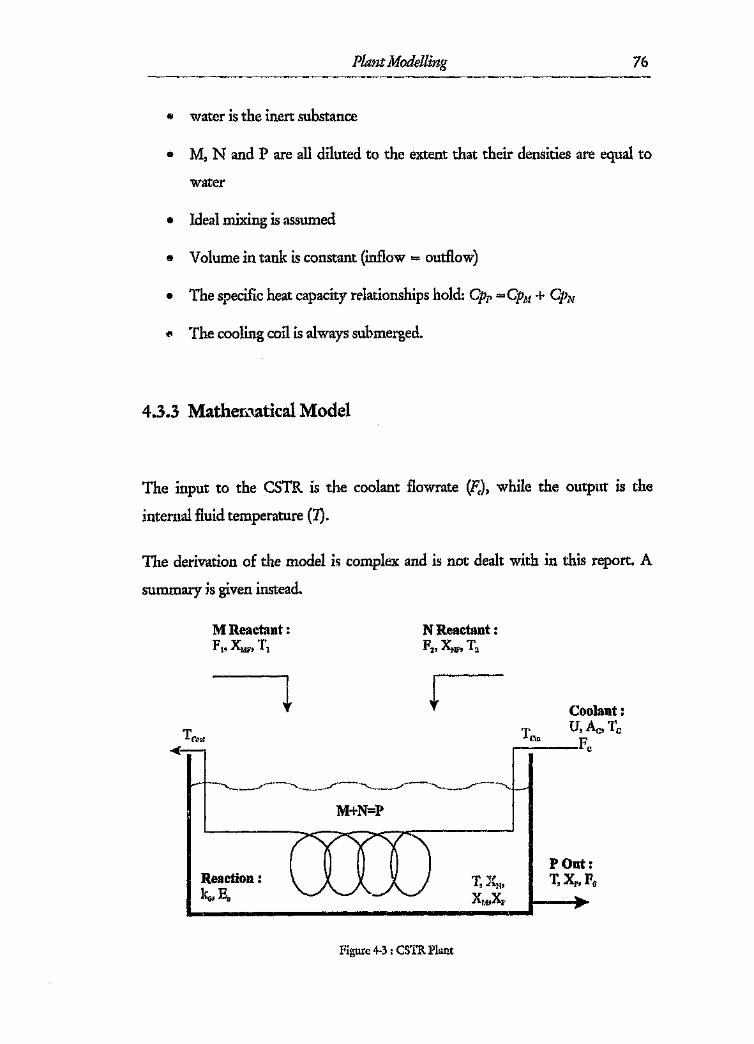
Plant Modelling 76
Ii' water is the inert substance
411 M, Nand P are all diluted to the extent that their densities are equal to
water
• Ideal mixing is assumed
" Volume in tank is constant (inHow = outflow)
• The specific heat capacity relationships hold: CPI' =Gpu + CPN
~ The cooling coil is always submerged.
4.3.3 Matheroatical Model
The input to the CSTR is the coolant flowrate lfc), while the output is the
internal fluid temperature (1).
The derivation of the model is complex and is not dealt with in this report. A
summary is given instead.
MRcactant:F1,XMjI, T1
NRcactant:Fz, XNF, T2
Coolant:TeiD Up' Ac, r,.----'c
M+N=P
fOr, x,x.x,
Reaction:1;:0' E.
Figure 4-3 : CSTR Plant

Plant Modelling 77
Summary 0/Operation,'
The CSTR consists of two input streams FI and ~ which supply diluted reactants
M and N. When reactants M and N come into contact (with a catalyst ifnecessary) an exothermic reaction occurs. The reaction is M + N => P. The inert
substance (water) together with the product P (with remaining unreacted
reactants left M and N) is removed (Po). As the reaction is exothermic, the
temperature must be controlled. This is achieved through the use of a cooling
coil, through which a cooling substrate flows (p''). Figure 4-4 shows the heat
released by the reaction as well as the heat removed by the coolant (linear
function of ~). For a steady state condition, the heat removed must be equal to
the heat added by the reaction. As can be seen, this results in three possible
operating points, The top and bottom point (P1 and PJ) are stable, while P2 is
unstable. Keeping the plant at this point is difficult as a slight deviation might
cause an increase in temperature, which in turn results in a higher reaction rate
and hence more heat released; leading to a rise in temperature.
;;Jij - - -I"·
~1»1
_ I I
P,
24lc-nro!:J:;;re(oc'1€t';C}
Figure 4·4 : CSTR Characteristic curve::...q removed by coil
+ - q formed by reaction
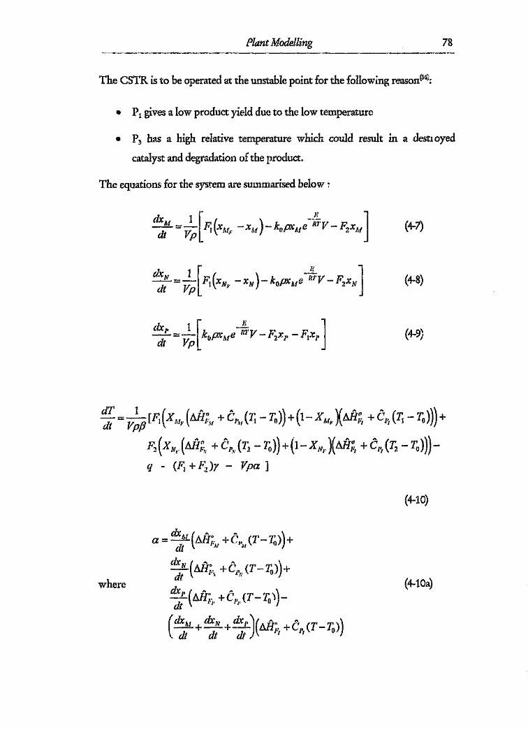
Plant Modelling 78
The CSTR is to be operated at the unstable point for the following reason(56i:
• P1 gives a low product yield due to the low temperature
o P" has a high relative temperature which could result in a destroyed
catalyst and degradation of the product.
The equations for the system are summarised below:
(4-7)
(4-8)
(4-9)
l~ :: V~p [11; (X u, (LVi;;\/ + CT1~Jr. - 7;})) + (1- X!lfF )( LVi;:/ + c; (r. - To))) +F2 (X Nt' (L'i1I;:'\ + C\, (7; - To)) + (1- X N1, )( illl;:j + (\ (7; -1~,)))--q - (F; + FJ)1 - Vpa]
(4-10)
where (4-10a)

Plant Modelling 79
(4-lOb)
r=xM(DiI;.. +[')' (T-To»)+.II .\I
xN(LVf;'~v +C/\ (T-Yo»)+(
A A \
X I' MI;'j. +Cpl'(T - To)} +
(1~xAf +XN +xl' )(AH;'i +c; (T - To»)
(4-lOc)
A detailed block diagram of this system is given in Appendix B. Figure 4-5
contains a simplified block diagram. This block diagram gives a better
understanding of the system and the interrelated properties.
Input!P.&F,
T
Ilea! Removed (q)
Figure 4-5 : Simplified block diagram of the CSTR
4.3.4 Parameter Values
The parameter values are chosen such that the steady state values are all achievable
by the available physical equipment'i" These are given ill Appendix A.
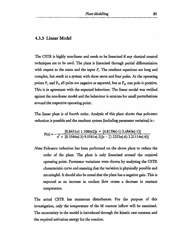
Plant Modelling 80
4.3.5 Linear Model
The CSTR is highly non-linear and needs to be linearised if any classical control
techniques are to be used. The plant is linearised through partial differentiation
with respect to the states and the input Fc' The resultant equations are long and
complex, but result in a system with three zeros and four poles. At the operating
points P I and P3' all poles are negative as expected, but at P2' one pole is positive.
This is in agreement with the expected behaviour. The linear model was verified
against the non-linear model and the behaviour is accurate for small perturbations
around the respective operating point.
The linear plant is of fourth order. Analysis of this plant shows that pole-zero
reduction is possible and the resultant system (including parameter variation) is :
pes) = -- S2 + [8.5546e(-3) 9,5561e(-3)]s - [1.3253e(-6) 3.21114e(-6)][8.8431el1.1080e2]s + [4.815ge(~1) S.6S40e(-1)]
Note: Pole-zero reduction has been performed on the above plant to reduce the
order of the plant. The plant is only linearised around the required
operating point. Parameter variations were chosen by analysing the CSTR
characteristic curve and ensuring that the variation is physically possible and
meaningful. It should also be noted that the plant has a negative gain. This is
expected as an increase in coolant flow causes a decrease in reactant
temperature.
The actual CSTR has numerous disturbances. For the purpose of this
investigation, only the temperature of the M reactant inflow will be examined.
The uncertainty in the model is introduced through the kinetic rate constant and
the required activation energy for the reaction.

Plant Modelling 81
4.4 Tank System
The tank system is chosen as a method of investigating dead time. Classical
control struggles with dead time as the control gains are linear. Fuzzy control
may offer some respite in this application as the control gains can be scheduled.
4.4.1 Rationale
The tank system is chosen as it illustrates a system which can have dead time. The
delay is assumed to be between the request for a change in flow and the actual
change in flow.
4.4.2 Assumptions
• Oscillations and ripples present on the surface are neglected.
The following assumptions are made in the derivation of the model:
• Laminar flow is assumed
• The valve characteristic is linear.
• The orifice equation is valid for tbis model.
• The density of the liquid is constant.

Plant Modelling 82'-~----~------'----
4.4.3 Limitations
This model is only used to highlight aspects of the control problem: and thus the
model might not reflect the practical system as it would be implemented.
4.4.4 Mathematical Model
The input to the plant is the control valve and the output is the tank level.
The control valve of the tank system is on the outlet. A tank system is a form of
capacity or integration. Thus the height of the tank can be given by :
h=-A1
j[qill-qlluIJit.p(4-11)
where qin and qOflt is the mass flowrate into and out of the tank respectively. The
tank is fed by an upstream supply with flow rate qiw This passes into the top of
the tank, giving the non-linear relationship:
(4-12)
where tt is the normalised valve position (0-+ 1).
The final equation for the tank (assuming a linear valve) is thus:
(4-13)
Dead time is included in the tank system. This dead time is implemented as a
delay between a request for a change in input flow and the response. This system

Plant Modelling 83
offers an ideal system to investigate dead time as it is a simple first order system
when linearised.
4.4.5 Physical Parameters
The physical parameters are chosen to represent a typical tank as would be found
in industry. The parameters are given in Appendix A.
4.4.6 Linearised plant
The tank system is linearised over all possible set point levels.
. [0.0422 0.0895].e-1d'\·P(s):::: s + [0.0093 0.0426]
The tank block diagram is given in Figure 4-6.
'Ij
-+i
i Tim~D~i;;ylI I
·····--[~~~~~~.~__I~.:.~~~~~)lai~.--~.-..~-.-------. i
II-.:i
Figure 4·6 : Ta11k block diagram

Plant Modelling 84
4.5 Miscellaneous plants
The following plants are also used in the investigation:
• FOPDT (First order plus dead time) system,
• nonminimum phase system.
These plants are used to investigate specific aspects of controllers.
The servo motor is a linear system with fast dynamics. Conflicting reports about
the role of fuzzy control with regard to linear systems makes this model
applicable for the investigation. The CSTR is a highly non-linear and unstable
plant. This plant is included in the investigation to highlight each controller's
ability to handle non-linear dynamics and large instability.
The tank system with dead time and various other systems are included to
illustrate specific control problems.

Controller Design and Comparison 85
5. Controller design and comparison
Chapter 4 introduced the models which are being used in the investigation. This
chapter summarises the design, implementation and results of the classical and
fuzzy controllers. First, the design methodology used for each of the QFT and
fuzzy controllers is presented. Then the controller design for each system is
discussed. The results and conclusions are given with a summary at the end.
5.1 Controller design approach
The aim of this investigation is to ensure a fair comparison between the classical
and fuzzy controllers. This requires that the information supplied to each
controller is the most appropriate for the control design methodology. This also
requires that the performance specifications chosen for each controller are equal
and have the same meaning. This aspect is not easy to achieve, as each design
technique requires the specification to be given in a different format. The classical
(QF1) meshed requires the specification bounds to be in terms of a required
frequency response! for whatever aspect of the plant the specification bound is
being imposed. For the fuzzy controller (which is not easily mapped into the
frequency domain), the specification bound is given as a qualitative requirement',
which will be met through iteration ..
Each design approach is discussed emphasising points which are relevant to this
particular study.
IOr the bounds Must be readily mapped into some form of frequency bound.
2 This is not true for ali forms of fuzzy controllers. Fuzzy controllers designed using a form of robust designtechnique can use some quantitative information in the design.

Controller Design and Comparison 86
5.1.1 QFT design
For QFT(35),like all classical techniques (except PID), a model is required of the
system to be controlled. The models need to be Iinearised around their respective
operating points. If more than one operating point is present, then this can be
included in the parameter variation (which leads to multiple plants). Some ..Jrm
of specification bounds are required for each system, These bounds vary
depending on the system and type of requirements. In the case of the S'~l'VO
motor, tracking bounds as well as robust stability and disturbance bounds are
required. In the CSTR, the tracking bounds are not necessary. In order to ensure
that the most is obtained from the classical approach, the bounds are made as tight
as possible, while still ensuring that the final control system is physically
realisable. Thus if the bounds are easily met with little gain, the bounds are made
more stringent. Simulation is used to verify that the controller meets the
performance specifications,
5.1.2 Fuzzy design
There is no specific methodology for designing and tuning a fuzzy logic
controller. These range from full a-priori knowledge with no tuning to on-line
adaptive fuzzy and hybrid systems. This investigation deals only with a manually
tuned fuzzy controller and fuzzy tuned classical controllers. Achptive fuzzy
systems often suffer from the problem inherent with neural networks : the final
controller, while working, does not disclose meaningful information about why
or what it is actually doing. In order for a fair comparison though, adaptive
classical control would need to be compared with adaptive fuzzy control.

Controller Design and Comparison 87
The fuzzy logic control design procedure followed is :
1. Define the system which must be controlled by specifying the inputs, outputs,
disturbances, sensors and system operating information available. Therefore
an overview of what must be controlled and the operating boundaries of the
system is required.
2. Define the control goals qualitatively and quantitatively. A~ a fuzzy system
cannot include the tracking or disturbance rejection bounds directly,
qr litative bounds are required. Quantitative bounds are needed to define the
required performance bounds. e.g. the step response must have a "time
constant" (a fuzzy system is non-linear and hence the time constant as defined
in the classical sense does not hold) of 10 seconds or the responsf. must be
within ~% of a set point after lOs. While these bounds cannot be directly
included, the fuzzy system car be tuned until they are achieved.
3. Understand the external dynamics of the system. This amounts to obtaining
the operator knowledge. For example, an operator who has used the system
manually, knows how the system responds to certain inputs. It should be
nc; 1 however, that operator knowledge is nUL;..i.wayseasily obtainable and
olen conflicting. This is, therefore, an "ideal" case when the operator
information is meaningful and easily extracted.
4. Define the type of inputs and outputs of the fuzzy controller. This includes
defining the required external dynamic components which determines
whether the output is an absolute value or an incremental one.
5. Define the universe of discourse ot the input and output. This includes the
range of values which must be included. These typically can be calculated
from external measurements or from design specifications.
(;i. Assign the fuzzy sets ·,vith their respective linguistic terms. The arrangement
of these sets is significant as the closer together the sets are, the finer the

Controller Design and Comparison 88
control which can be implemented resulting in a greater complexity. For large
fuzzy control input signals, the sets can be spaced far apart, U3 the exact value
of the current plant output is not. significant, aside from the fact that the
deviation from the setpoint is large, Typically the nwnber of sets is three, five
or seven. More sets and linguistic terms can be added later.
7. Assign the FAM bank or rule base. This is obtained Irorn converting the
knowledge gained from the operator (in step 3) into a set of rules.
8. The methods of fuzzification, connection, aggregation, implication and
defuzzification need to be defined (seeChapter L).
9. Generate the control surface. Every possible output, for every possible input
(over the universe of discourse) is shown in this surface, and hence the action
is deterministic. It is therefore possible for .he designer to have complete
control over all areas of the control surface. By examining the control surface
carefully, it is possible to identify any areas where the control is inappropriate
or missing. The magnitude of the output is important and it should be noted
whether the entire input and output space has been accounted for. It is typical
of some defuzzification methods (e.g. centroid), not to use the entire range of
the output space. This is due to the effect of averaging. This is compensated
for by increasing the output space.
10. Simulate and tune the fuzzy controller until it is within the desired
specification bounds. Tuning is usually difficult and reqUIres numerous
simulations. There are various methods which are employed in this
investigation:
• Examine the trajectory of the system plc tted on the control surface.
(i.e. a plot of Error vs. dError). Areas where the response is slow or not
understood can be clearly seen and corrective action taken.

Controller Design and Comparison 89
• Change the output sets ( if the input set positions are understood to be
correct and meaningful ), such that more or less control action is
applied at certain regions,
• Modify the rules when the action taken is clearly inappropriate for the
situation.
5.2 Controller specification and design
A controller for each plant is defined which satisfies given performance bounds.
The actual controllers and their respective plots (either Nichols or control
surfaces) are given in Appendix C (unless directly relevant).
5.2.1 Servo motor
Aim: To determine the controller's ability to deal with a well defined linear
plant, as well as clearly defined tracking bounds.
Plant Input: Signal voltage to amplifier
Output.' Motor angular position (in degrees)
5.2.1.1 plant model
The plant model for the QFT design case is described in Chapter 3. For the fuzzydesign, however, the model needs to be converted into a qualitative one such that

Controller Design and Comparison 90--------------~-
control rules can be obtained. Through a series of step tests it is possible to
qualitatively determine what voltage results in what motor speed. From this, the
input and output ranges, as well as the rules were generated.
5.2.12 QFTspecifications and design
The servomotor model is summarised in (5~1):
pes) = s2+[613 673]s+[3.1c4 6.4e4][7.6e5 1.2e6]
(5~1)
As can be seen, the motor model is second order and linear. The specification
bounds chosen for the step response are such that, ideally, the amplifier will not
saturate when the desired tracking is obtained. This was achieved through
analysing the ma., -.num speed to which the system could respond, assuming
limited voltage bounds. 'XTiththe parameter variation, the fast poles varies from
around ~50 rad/s to ~110 rad/s. This is a large model uncertainty to take into
account and should test the controllers significantly.
The QFT method is ideal for this plant as it is already linear) and the specification
bounds have been clearly defined. The bounds are summarised below:
• Tracking bounds: TJ~,(8):S; IT(s)F(s)l::; TF;,(s) (5~2)
where TF~.cs)=: i +2.(0.85).(100) + 1002 (S~2a)
and TIt;, (s):=: i +2. (0.65). (150) + 1502 (S-2b)

Controller Design and Comparison 91-----~--~------~--------~---
8 Robust stability: IT(s)1 S; 1.2 (5-3)
The final controller is :
s-~~+1G(s) := 0.295 127,,7 --~
( s )( s )5461+1 ,8357 +1
(54)
5.2.1.3 Fuzzy specifications and design
The fuzzy system specification bounds are given below:
• Tracking bounds: Track ,1. 10Hz sine wave (amplitude 180°) to within 5 %.
• Step Response: Reach 5% of set point value within 0.075 ('t' :::1 0.026s).
The tracking bounds are a test of the bandwidth of both systems. The QFT
bound is such that the servo -notor will track a 10Hz wave as well. The step
response bound is a qualitative interpretation of the QFT bound.
The controller choices and control surface are given in Appendix C. Centroid
defuzzification was used as the output is smoother than that obtained from other
methods.
To determine the rules, knowledge vf the servo motor's response to certain
voltages is required. This qualitative knowkdgc w?s obtained from step tests on
the simulation model. The operator knowledge together with logical reasoning
produced the FAM bank.
Increasing the voltage in any direction (positive or negative) causes the motor's
rotational speed to increase, therefore causing the angular position to change

Controller j)esign and Comparison 92
faster', The rules, based on this model can be generated. E.g. If the error is
positive and large (PM) and the servo motor is moving to increase this error (PM
or PS), then make the voltage such that it will change the direction and reduce the
error (PL)
5.2.2 CSTR plant
Aim: To test the ccntrollers on an unstable and highly non-linear plant.
Plant Input: Coolant flow
Output: Temperature of internal fluid
Disturbance: Temperature of incoming M reactant.
5.2.2.1 Plant model
The plant model for the QFT design case is described in Chapter 3. For the fuzzy
design, however, the model needs to be convened into a qualitative one such that
control rules can be obtained. The qualitative model of the CSTR is harder to
obtain than for the servo motor model. This is due to the operating point being
unstable. The operating point is obtained from examining the behaviour of the
plant. At temperatures above P2 (see Chapter 4), the temperature rises to a stable
point, and below P2' the temperature drops to another stable point. From this, an
approximate J"'_ rating point can be obtained. The maximum and minimum
I This is a qualitative interpretation of (5.1).
2 Due to the convention used, a PL voltage results in a PM error eventually.

I
'.
Controller Design and Comparison 93
coolant flowrates', and the possible temperature values are used to determine the
input and output bounds.
5.2.2.2 QFT design
The plant with parameter variation can be summarised in the form of a transfer
function as :
[8.8431el 1.1080e2]s + [4.815ge(-1) 5.6840e(-1)]pes) == - S2 + [8.5546e(-3) 9.5561e(-3)js - [1.3253e(-6) 3.21114e(-6)]
(5-5)
Note: Pole-Zero reduction has been performed on the above plant to reduce the
order of the plant. It should also be noted that the plant has a negative gain.
This is expected as an increase in coolant flowrate cause, a decrease in
reactant temper ature. In the design of the controllers, this negative sign is
ignored and instead, the gain signs are interchanged at the feedback error
calculation.
The plant system is slow with a step time constant in the region of 15 minutes.
The QFT design procedure followed involved choosing the specification bounds
and designing the controller. If the specification bounds were too tight and the
designed controller saturated the valve too quickly, the bound specifications were
reduced until the control action was physically realistic. This specification
method is used such that the controller design could be considered the best
1 The maximum and minimum flow rate are not the bounds of the fuzzy output range as the change in flowrate is the output. These values serve to indicate a rough value for the maximum rate of change which isused.

Controller Design and Comparison 94
achievable with a linear controller under the given conditions. This is important
as the fuzzy controller does not use bounds for its design as does the QFT,
therefore an optimal linear controller design is required for a comparison. The
specification for the controller design are:
, . I I i + 0.1 0 Is + 1 X 10⁻⁴Robust output disturbance bound: S(s)::::; 3 201' 02 1 10-'~{+ . s: + 1. s+ x ~
(5-6)
Robust stability bound: 18(8)1:::; 1.2 (5-7)
The robust stability bound corresponds to a phase margin of approximately 46°
and a gail! margin of 15dB. The gain margin is large as the CSTR is a highly non-
linear system, and this specification will enforce a higher robustness to model
parameter variations. A steady state error is allowed as this problem is a
disturbance rejection one and not a tracking problem. Thus no integrator is
required in the controller.
The plant is obviously unstable (due to the positive pole), and hence stabilising
the CSTR is a primary objective. No input disturbance rejection is specified, as a
specification on the output disturbance bound places limitations on the input
bound. Any input disturbance can be converted into an output disturbance, so
this is not seen as a limi: ing choice.
The controller designed is :
T 1G(S) = 0.001789 ( . s ')(-,-S' --)
1321 +1 3.631 +1
(5-8)
The Nichols plot of the plant, with the controller is given in Appendix C.

Controller Design and Comparison 95
5.2.2.3 Fuzzy Design
The fuzzy system is well suited to this system and the generation of the required
rules was easily achieved" The bounds for the CSTR are hard to quantify in terms
of a fuzzy controller, but they are given below:
• Stable
• Disturbance rejection: minimise the effect of all disturbances to within 1 % of
the set point within 100 seconds.
The disturbance rejection bound is a qualitative interpretation of the same bound
(in the frequency domain) given in the QFT design. This is obtained from
mapping the frequency domain bound into the time domain and examining
exactly what is required.
The choice of fuzzy system and the control surface is given in Appendix C. This
particular problem cannot be solved by a fuzzy system alone. If the output of the
fuzzy system is defined as the actual flowrate, the problem cannot be robustly
solved, for if the equilibrium point coolant flow rate is not constant and exact, the
fuzzy output is useless, and oscillations will result. The fuzzy output must
therefore be an incremental change in the flow rate. For this to be realisable, an
integrator is required after the fuzzy system, and hence a dynamic system is
required.
The rules chosen for this problem are logical and based on how the CSTR
responds to changes in coolant flow (step tests).
An increase in coolant flow causes the temperature to drop quickly. Therefore the
following rule would be logical: If the temperature is too high (error is PM) and
there is no change in the temperature, then the valve should be opened fast (open
fast), such that temperature drops (increase coolant flow).

Controller Design and Comparison 96
5.2.3 Tank system
Aim: The aim of the tank system is to investigate the controller's ability to
control a system with dead time.
Plant Input :Output flow rate.
Output: Level of water in the tai '.:.
5.2.3.1 Plant model
The plant model for the QFT design case is described in Chapter 3. The fuzzy
model is easy to determine since the system's response to change in input is
obvious (seesection 5.2.3.3).
5.2.3.2 QFT design
Numerous possible equilibrium points for different levels in the tank are used to
obtain the parameter variation in the plant. The controller is designed for the
tank model in (4d13) with dead time added (td=5s). The dead time introduces
significant lag onto the system. The dead time has converted a first order system
which is easy to control into a complex and difficult control problem. Like 1\1MP
systems, the dead time limits the maximum gain which can be added to the
system. The specifications only call for a stable system with as much open loop

Controller Design and Comparison 97--- --~-~.------~-
gain as is permissible. Meeting any additional specifications becomes secondary to
stabilising the system. The final controller is :
s--+1
G(s) = 0.03115 Q.0229
SC~~O+ 1)(5-9)
5.2.3.3 Fuzzy control
Like the QFT system, the aim with the fuzzy controller is to stabilise the system
and yet provide a fast response with as little oscillation as possible. Steady state
error was allowed in the system to try and prevent oscillation when the system
was near the equilibrium point. The rules were obtained though logic, but trying
to include the time delay into a rule is very difficult. The rules are typically
independent of time! and therefore taking time into account is difficult.
An increase in flow rate means that the tank will empty faster than before, and
the level will drop. A suitable rule would therefore be : if the level is too high
(NM) and there is no change ill the level, then open the valve fast (open fast) to
bring the level back down. As can be seen, the linguistic term "open fast" must
take the time delay into account.
IUnless a clock becomes the input to the fuzzy controller.

Controller Design and Comparison 98
5.3 Controller design and comparison for specific aspects
of plants
The plants discussed in this section are theoretical plants which are included to
illustrate certain aspects of the control problem. Although the plants are
theoretical, they do represent physical plant characteristics.
5.3.1 Non-minimum phase plant
Designing a linear controller to control a non-minimum phase plant in a feedback
loop is difficult. This is a system with a positive zero. High gain causes the stable
poles to move towards the positive zero, which causes instability. To illustrate
this concept, consider the following plant,
(s-7)P(s)-
(s+3)(s+4)(5-10)
Figure 5-1, shows the Nichols plot of the system.

Controller Design and Comparison 99
.31) ·2Si) ·1(~X:H."(oc1''''l Y:r.lli;-{~)
.100
Figure 5-1 : Nichols plot of non-minimum phase plant
The RHP (right hand plane) zero has the property of providing lag with
magnitude increase. Therefore if we try to reduce the lag through adding a LHP
zero, the resultant is a system with finite gain at infinite frequency (unrealisable
solution). Adding more LHP poles to prevent this results in too much lag. The
result is that a RHP zero provides an upper limit on the rain crossover frequency
Wc and the low frequency feedback benefits are minimised.
Examining the plant given by (5-10), the maximum gain which can be applied is 7
before the system becomes unstable. A gain of 2.69 is required if the robust
stability margin of IT{s) I< 1.2 is to be achieved. The steady state error for the
system with a gain of 5 (small oscillations, but stable) is still around 25%, which is
unacceptably high. Loop shaping is possible but as discussed before, it is
extremely difficult with little benefit. Adding an integrator introduces another
phase lag of 90°, therefore restricting the maximum gain to 1.7. This ensures no
steady state error, but oscillations are present. The NMP has limited the ability to
achieve the maximum benefits of the linear controller.
The fuzzy controller approach is well svited to this problem. Due to the fuzzy
system's non-linear characteristics the problem is avoided. A fuzzy controller for

Controller Design and Comparison. 100------------_._---
the above system is easy and quick to design. The knowledge which was used in
the design was the black box step test. From this, the only indication that the
system is more complex than a first order, or damped second order system, is the
initial negative respons? of the system. Using the time constant of the system,
ranges for the change in error are quantified, as well as the error range and the
control action range. The rules are straightforward and logical. It is assumed for
this problem, that saturation is not present in the control action. The output of
the fuzzy controller is actually a change in the required control action, hence, the
output is passed through an integrator before reaching the plant (s{'e section
5.2.2.3 011 the CSTR). The initial fuzzy system was conservative and a slow step
response resulted. After a few iterations, the step response had an acceptable rise
time with zero steady state error. The fact that the system is NMP had little effect
on the controller design.
No literature has been found on applying the fuzzy control technique to NMP
plants, As has been shown, fuzzy control may provide a quick and accurate tool
for control of such plants and should be investigated with further research. The
controller information is given in Appendix C.
Note: the fuzzy controller is 110t the optimal, nor does it ensure the fastest
response. Itmerely illustrates the point that this is a situation ideally suited
for ~ fuzzy controller. The response can be made faster (essentially, as the
gain is non-linea,', the step response time constant could be made infinitely
small, assuming no saturation). The problem, also found with the servo
motor controller, is that the fuzzy controller becomes difficult to tune
when very fast responses are required, as the overshoot must be prevented.
The aim of this problem is to show that the problem of NMP which
omplicatcs linear controller design can be easily overcome dUf' to the
non-linear nature cf the fuzzy controller.
The step respon~~sfor the two controllers are given in Figure 5-2 :

Controller Design and Comparison 101
15 -~-T-'·--~· - '-"~---'-'-'-r----~---r~-----'--~~-'-[--'-----T------
1
0$
____. ..i- _____ .._.i __ .. _-----Il " In IJ "'"
1:;;J
r~:"7c~:,';i,i::Jr &'~S,-'::::1~-~-r"-""-----'- ---'~'-"-'-'I
-- __ l_· ____ ···~
I. .- - - _. _I
,I
1 '--1
1
fO 1, 14 I, 15 mTIfJ
Figure 5-2 : Step response of the QFT and fuzzycontrollers for a non-minimum phase plant.
5.3.2 Highly non-linear plant
A highly non-linear plant (asymptotically unstable) is :
.tl == Xl'jX2 :::: u+ P.Xi
(5-11)
where Z"> O.
The system is highly unstable and approaches infinity in under 2 seconds
(depending on the value of P). The plant is easily Iinearised, but analysis of the
linear plant around the operating point (x!=O), shows that the variation in the
model behaviour for different initial conditions is large; and hence the QFT
technique requires use of all LTIE set(51l.The plant is, however, easily stabilised
using state feedback.

Controller Design and Comparison 102---- -~---".---
Designing a fuzzy controller for this plant is not easy. A fuzzy controller for the
situation when P= 1, was obtained and this stabilises the plant effectively. It is not
possible however, to stabilise the plant when P= 10 as the plant instability is too
fast, and it is difficult to track, "catch" and counter the response fast enough.
Theoretically, the fuzzy system should be able to stabilise the system, but the
design is difficult.
The conclusion reached from this controller design is that jf the plant can be
accurately modelled, linear feedback control, possibly with state feedback, offers a
better solution. The system could arguably be controlled through fuzzy control,
if access could be gained to the inner parts of the system that is state feedback
with fuzzy control.
5.3.3 Hybrid control of a first order plant with dead tirne
Dead time is a 111\1jorproblem in physical plants, and is present in numerous
industrial process planes. The presence of dead time necessitates the lowering of
the controller gain to maintain stability. Many methods have been proposed to
counter dead time, including:
• Smith predictor(:iB)
• analytical r ,dictor{59)
• general purpose algorir'im (Gautam and Mutharasan)(59)
The design proposed in this section is a hybrid controller comprising a Smith
predictor which is tuned by a fuzzy controller.
The Smith predictor is the best known dead time compensation technique and is
extensively used in industry(5S,59).It is model based and should ideally be

Controller Design and Comparison 103-~-----~----
implemented digitally. The development of the theory of the Smith predictor is
not given here, but Deshpande and Ash(59)et al give a good summary.
Consider a first order plant with dead time:
(5-12)
where K, is the process gain
ttl is the dead time and
r is the process time constant.
This system could represent numerous physical systems including a tank level,
conveyor system or a stirred tank (temperature).
MacLeod(45)developed a hybrid fuzzy-PID Smith predictor system which used a
similar first order system (conveyor belt). His fuzzy system tuned the gain of the
PI controller depending on the actual plant gain. The method of control posed in
this investigation is similar. Although the Smith predictor is a powerful control
technique, it does have problems. If the dead time is not known accurately and
hence differs from the actual dead time of the plant, then the system performance
degrades, and becomes worse the more inaccurate the estimate is. In order to
improve the robustness of the Smith predictor, it is proposed that a fuzzy system
be used to modify the dead time of the predictor such that it minimises the delay
error. A block diagram of a Smith predictor, including the adaptive fuzzy
proposal, is given in Figure 5-3.

Controller Design and Comparison 104
R(s)_ {:X:)" ... t('\/ ')s.J,," \/. \/ i- t - t .
Figure 5-3 : Adaptive Smith predictor control scheme
The problem with tuning the dead time is that if the system is in steady state, the
effect of the discrepancy will not be noticed until there is a step change or a
disturbance. Therefore, in order to tune the system, a series of step changes is
required. It is from these step changes that the tuning occurs. The fuzzy system
has two inputs, namely the plant output and the predictor output (both after the
delays). The output of the fuzzy system is the incremental change in the predictor
time delay estimation. The principle on which the system works is :
* The system must be near steady state and be stable. This means that the
predictor must have a reasonable guess of the actual delay, such that the
system can move to a steady state condition.
• When a tuning step is applied, the plant output and the predictor output are
examined by the fuzzy controller.
• The actual magnitude of the outputs IS not important provided the step is
above the specified noise threshold value in the fuzzy system. This means that

Controller Design and Comparison 105
the system need not be in perfect equilibrium and hence disturbances and
noise will not affect the tuning of the system provided they remain below this
noise threshold value. What is important is the timing of the two inputs. If
one of the step responses occurs before the other, then the predictor value of
the time delay is incremented accordingly.
• The system will also be independent of changes in the plant parameters. As
discussed above, it is only the timing and the threshold values which are
important.
.. This system will only change the time delay on the positive part of the step.
This can be changed if a faster tuned system is required, but the system
complexity will increase.
The method of tuning the system is not seen as impractical. It is obviously suited
to a system which is continually changing for example a tracking system. The
tuning mechanism can be made to work with other forms of signals including a
sine wave. In a disturbance rejection problem, the method proposed is aimed at a
plant where the operator has noticed that the system performance is not optimal,
and by running the s\,eptuning, they can readjust the dead time compensator, The
changes in the actual dead time value will only occur when the tuning is started
and not during normal operation. Unless the disi urbance can be measured, there
is no inherent method of tuning the dead time. If the disturbance can be
measured, then a system similar to the one above may be possible, where the
disturbance forms an input to the fuzzy system.
The results of the simulations were excellent and showed the fuzzy system tuning
the dead time accurately. It must be remembered, however, that this is a
simulation and the plant is only a first order system.
Figure 5-4, shows the step tuning for the system. The actual dead time is 6
seconds, but the initial predictor estimate is 4 seconds. The severe oscillation for
100 < t < 200 indicates the problem inherent with Smith predictors when the
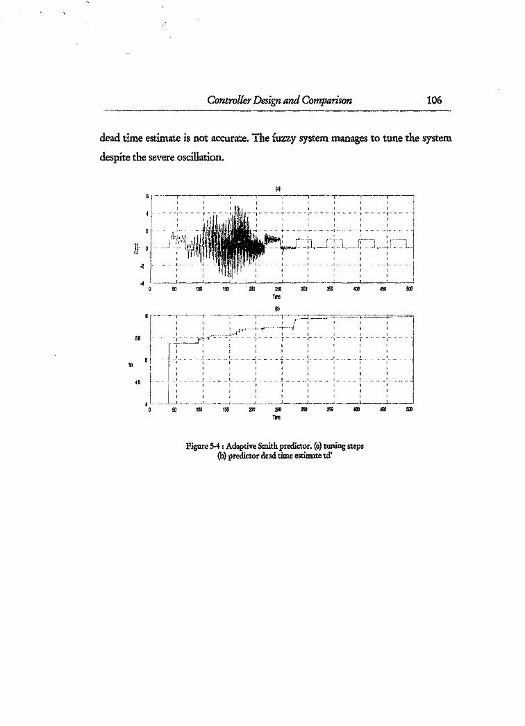
Controller Design and Comparison 106
dead time estimate is not accurate, The fuzzy system manages to tune the system
despite the severe oscillation.
('J
n-cs
·2
-450 100 150 200 250 £~ 3W 400 450 [Xl)
T'l"iI
(b)
55
I ..I
~ I
45 ... I
I
ill 100 150 200 2'"Ji) 300 350 400 450 500TI!1"~
Figure 5·4 : Adaptive Smith predictor. (a) tuning steps(b) predictor dead time estimate td'

Controller Design and Comparison 107
5.4 Simulation comparisons
Section 5.4 summarises the results of the comparisons between the fuzzy and
classical controllers. The comparisons are limited to specific control .esign
aspects, and a more general comparison about design issues is given in section 55.
5.4.1 Tracking
Servomotor: This forms the basic test for the comparison. The QFT controller
performs deterministically and is within the bounds as is expected for aU of the
plants. In contrast to this is the fuzzy controlled serve ir. While the nominal
plant meets the specifications well (an even a bett lonse than the linear
controller), the performance variation of the other plants is significant, with some
having large overshoot and others critically damped. This is Obviously a great
limitation of the fuzzy approach, as model uncertainty is very difficult to control
within the specification bounds (and its effect is unpredictable). Although it ispossible to ensure that it is within the bounds, it takes a large amount of time to
tune the controller to that degree .without using some form of training
mechanism (e.g. neural networks).
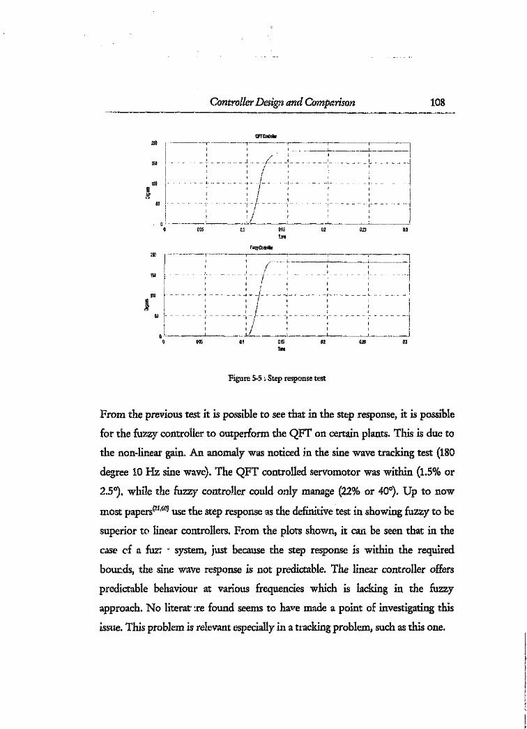
Controller Design and Comparison 108
.,
DIi5 0.1 0.15 02 DiS 02Ere
fllZrjComrllerlIB
15U
lro ./
'"I
Jr/
50 .. --i·· - - .- - - " -
0115 01 0.15 02 025 03Time
Figure 5·5 ; Step response test
From the previous test it is possible to see that in the step response, it is possible
for the fuzzy controller to outperform the QFT on certain plants. This is due to
the non-linear gain. An anomaly was noticed in the sine wave tracking test (180
degree 10 Hz sine wave). The QFT controlled servomotor was within (1.5% or
2.5°), while the fuzzy controller could only manage (22% or 40°). Up to now
most papers(21,60)use the step response as the definitive test in showing fuzzy to be
superior to linear controllers. From the plots shown, it can be seen that in the
case cf a fuz: " system, just because the step response is within the required
bounds, the sine wave response is not predictable. The linear controller offers
predictable behaviour at various frequencies which is lacking in the fuzzy
approach. No literar :re found seems to have made a point of investigating this
issue. This problem is relevant especially in a tracking problem, such as this one.

Controller Design and Comparison 109
£00
IW
-_..-···-~~-·-t----'-·--·-----i-~~~-~,--------,-·--~'_m---- ..--_
'. '. /. '\' '/-\ ' II I \ I I I i
,\ .... ,." r . '\! _, _,1.; __ \'. '.. ...,).I I I I ' I '
\ ' , ; \ ' , '\' I\ ,I \1 If I\ I -\ -/ \ - I:
\ /" '\ ( '\ II. \" /\ /~ '\ _j, - \ II\ I' '\ I ,I I'/' '\; ,\1I~ I ,II I/J____ -= -' __ ~ ~ ;___~ ~__L '::______
0.1 0.15T"",
01 025 03
100
OI, 0.1 015T",
02 025 0.3
Figure 5-6 : Sine wave tracking test
CSTR : While the problem is inherently one of disturbance rejection, the step
response forms a common and simple method for comparison between the two
systems. The fuzzy controller showed an excellent step response with a fast rise
time and no oscillation, even outside the operating point. What should be evident
in the response, however, is a "bend" in the step response when in the vicinity of
the set point. This is due to the "braking" rules being fired, which slow down the
response when approaching the set point. The QFT, as expected, works well
within the operating point bounds: but oscillates outside this point. This problem
highlights the advantage of this fuzzy approach, namely that the rules can take in
a wider operating region. With QFT control, all the operating regions must be
included in the design stage. The precise bounds of the operating region are not
clearly defined in the fuzzy design approach 1whereas the operating region bounds
in the QFT design are dearly defined before simulation.
1Unless a "robust" fuzzy design technique is used.

Controller Design and Comparison 110
27.2
27
20.8
20.6!
2D.4
2,2
2~
272
27
-! ". - - 258
.2li.n"E.'" ZlI4
262
204~) 500
06
(d)
ea
(el
08
06
- .1
1
. __ 1__ ___ ___J -
I
- -- - ~I- ...
I
.1 ~1 I _"
I I
oo 100 200 300
Time100 ,00 :lilJ
TiThl
Figure 5-7 : Step test on CSl'R.(a) - QFT controller step response;(b) - fuzzy controller step response;
(c) - control action for QFT controller;(d) - control action for fuzzy controller.
5.4.2 Disturbance rejection
CSTR: The disturbance applied is a step in temperature of the M reactant inflow.
Both controllers rejected the disturbance well. The QFT controller settled to a
new operating point within a few minutes, but the new point was 0.02 degrees
(0.001%) off the set point. The fuzzy controller limited the set point change to
within 0.003 of a degree before settling down slowly. Thus it can be concluded
that both controllers rejected the disturbance (which was a significant one)
effectively.

Controller Design and Comparison 111
26.011
_L _L
2CJ!7
r~~e((5;,j
leo
26057
Figure 5-8 : Step dista; b~nee rejection test results
A time varying disturbance was also tested. Again the temperature of the M
reactant inflow was changed through a O.otHz Sill wave of magnitude 2°. Again
both controllers maintained the CSTR within acceptable bounds, with the fuzzy
controller deviating slightly less.

Controller Design and Comparison 112
fj Z6G~
r~~ 2~,'E
~G,07j
1G.Q3
1-301
4S·J ~mTLT!3
100
~G.OO
2G.t61
~ L5_V..3
"-u"'2B.1l51
2GJ1'JJ
Figure 5-9 : Time varying disturbance test results
5.4.3 Noise suppression
Servo: Normally distributed band limited noise was used in the tests. Various
frequency bands were used from 10Hz to 200Hz. In all cases, the fuzzy system
exhibits "lightly better noise rejection than the linear system does. The
improvement varies from negligible (25Hz-150Hz) to a 50% reduction in response
(100Hz-200Hz). It is possible that each controller could exhibit better behavi ; ifdesigned differently, but it is believed that fuzzy control will allow better noise
rejection due to its non-linear nature which allows more flexibility with
scheduling the gains.
Figure 5-10 is a plot of both controller's noise response (50Hz-+150Hz) of mean
zero and standard deviation 0.4023. The QFT controlled system has a high
bandwidth which results in the noise having a significant effect on the system
output. The noise causes the QFT controller to continually saturate the amplifier,
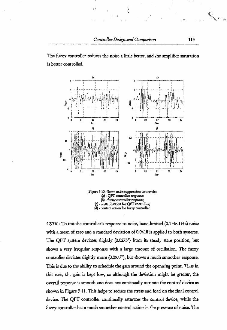
Controller Design and Comparison 113
The fuzzy controller reduces the noise a little better, and che amplifier saturation
is better cont rolled.
r1 nl~
03 03·2 ·1
..j ·201 02 0.3 0.4 0.1 02 03 0.4
Ticl Time
(e) (d)
020.5
f,r 8.;.]
'" ~'>
·D5·0.2
.1~I 0.2 0.3 0.4 0.1 02 0.3 0.4
Tem TL11l'
(a) (11)
Figure 5-10 ; Serve noise suppression test results(a) • QFT controller response;(b) • fuzzy controller response;
(,~)- control action for QFT controller,(d) - control action for fuzzy controller.
CSTR .'To test the controller's response to noise) band-limited (0.lHz-1Hz) noise
with a mean of zero and a standard deviation of 0.0418 is applied to both systems.
The QFT syster~'1deviates slightly (0.0273°) from its steady state position, but
shows a very irregular response with a large amount of oscillation. The fuzzy
controller deviates slig~,tiymore (0.0977°), but shows a much smoother response.
This is due to the ability to schedule the gain around the operating point. '1"'1.1I.1S in
this case, tl-. gain is kept low, so although the deviation might be greater, the
overall response is smooth and does not continually saturate the control device as
shown in Figure ~~·11.This helps to reduce the stress and load on the final control
device. The QFT controller continually saturates the control device, while the
fuzzy controller has a much smoother control action in •.I.~epl'esence of noise. The

Controller Design and Comparison 114~-------.----------windowing' technique offers a possible method of reducing the systems noise
sensitivity, as the gains around the operating point can be accurately set up to
"filter" out most of th ! noise. This offers a possible future research topic.
(a) ~)
2S.frl
20.1
511 ''10Tune
150
.• 0.4..)"i:
~ 02
08
£505
go
"".6
50 100 ~50 200T"1e
(eJ
08
0.6
"",04
102
50 il't f5ll a~lime
Figure 5-11: CSTR noise suppression test results(a) - QFT controller response:(b) - fuzzy controller response;
(c) - control action for QFT controller;(c) - control action for fuzzy controller.
~I 5.4.4 Unmcdelled dynamics/model variation
C:JTR : The unmodelled parameter variation tesc involves setting a new operating
coin, for the system. Both controllers manage to achieve this for the nominal
plant, but the fuzzy system does not have any oscillations. Thus this advantage of
I The windowing technique uses (at least) two fuzzy controllers. The first controller is used when the error IS
large and therefore gives coarse control. When the error is below a certain threshold, control is passed overto the other fuzzy controller which administers fine control over the plant. This allows individualcontrollers to be optimised for different areas of the operating region .
..

Controller Design and Comparison 115
the fuzzy system is illustrated, namely that it can be more robust over a great
variety of conditions as it is not designed for a specific case as is the QFT
controller'. This has a great implication when the uncertainty is large or the ideal
operating point of a system is not known. Both systems had trouble controlling
the plant when large unmodelled parameter variation is used or there are large set
point changes (QFT can handle this, but must be explicitly designed for it).
Analysis of the characteristic curve indicates that the system is very non-linear at
these points (small changes in coolant flow cause large variations in temperature)
and the controllers tend to overshoot due to this problem. The fuzzy system
cannot deal with this situation well as the req-iired actions are different when
approaching the extremities of the curve. Start up and shut down of a system like
this would normally be done by an operator, or it could be performed by another
fuzzy system. This demonstrates the area when fuzzy system design becomes
problematic. If the rules governing the control of a system are not constant, but
change depending on the system state, then multiple fuzzy systems must be used.
5.4.5 Non-minimum phase
The non-minimum phase plant was investigated in section 5.- -"The outcome of
this investigation is that the fuzzy controller offered an excellent method of
overcoming one of the limitations of classical control. The rules which are used
for the non-minimum phase plant are similar to those for a minimum phase plant,
and hence the design was relatively simple.
1The problem with the fuzzy approach, however, is that the response is not us predictable as it is with theclassical approach.

Controller Design and Comparison 116------_._-----._----
5.4.6 Dead time
Tank: The tank. system developed is used to investigate the control of dead time.
The classical system is straightforward to design, but as expected, the feedback •
benefits are severely limited by the nature of dead time (phase lag). The fuzzy
system, however, is 110tas easy to design. Defining the rules for a system with
dead time is harder than for a system without dead time. This is logical since it is
easier for an operator to control a simple process with no dead time, and hence
reduce the action to rules, than it is to control a simple action with dead time.
T' e actual rules become difficult to define and are plant specific. If the delay is a
certain length, then the braking rules need to be defined such that they are fired
when the plant reaches a certain part in its Error/dlirror trajectory. If the plant
changes, the required position of these braking rules changes and hence
oscillations occur. In the classical case, plant variations can be easily taken into
account, although the variation cannot always be reduced to the desired levels.
This can be seen with the fuzzy controller. The level fer which the fuzzy
controller is designed works well (but allowed a steady state error), but when a
different level set point is specified, then oscillations are present. Neither
controller is robust or offers any meaningful control. The classical approach has
the advantage of a clear representation of what the controller will achieve, while
the fuzzy approach allows non-linear gains to achieve better performance. The
conclusion reached from this is that neither system is suited and a time delay
compensation technique is required.

Controller Design and Comparison 117
15
01
J -- -- ----- --- _-o
-.---_j_~~--------
Figure 5-12: Dead time step response test
Hybrid: As discussed earlier, the hybrid system offers exceptional robustness in a
dead time situation, and therefore shows a good combination of qualitative and
quantitative k.iowledge in the controller design. The control offered is far
superior to either of the systems on their own, with a little added complexity.
5.5 Design Comparison,I
The following is a summary of the similarities and differences between the
classical and fuzzy control design techniques.

Controller Design and Comparison 118~---------------
Table 5·1 : Comparison between fuzzy and classicalcontrol design
Aspect Fuzzy DesignClassical Design
Par~eter A classical design technique Fuzzy control IS now startiag to
variation and such as QFT allows formally be able to handle parameter
uncertainty structured and unstructured variation through robust design
uncertainty to be easily taken techniques (using Sugeno style fuzzy
into account. systems) and usmg fuzzy numbers.
Specification of the fuzzy sets and
numbers is not definite and hence the
experience of the designer plays a large
role 111 the quality of the hlZZY
. controller. The fuzzy number method
of handling uncertainty is not well used,
and instead the uncertainty 15
incorporated into the fuzzy sets on the
universe of discourse.
Frequency
information
The classical design The fuzzy system offers no method of
technique uses frequency incorporatir-z frequency information
information directly in the directly into the design. Should there be
design _ through transfer some specific information which IS
functions', important and must be included,
external dynamic elements are required
(frequency analyser, differentiator etc},
I Or a variation of them e.g, state space.

Controller Design and Comparison 119
Design
Choices
Optimal
controllers
Table 5-1 (cont.): Comparison between fuzzy andclassical control design
Clear and definite design
option; with well
documented implications
characterise the classical
The designoptions in a fuzzy controller
are numerous and their effect ill-understood. This could be interpreted as
a fuzzy controller having greater
flexibility, and this is true, but their
effectsare not easilypredictable.
designtechnique.
In the QFT approach the There is no optimal controller m a
optimal controller is one fuzzy system ( if complexity is ignored
which meets all the). In theory, the fuzzy controller can
specifications exactly and provide control which is optimal, in the
"hugs" the required stability sense that no other form of controller
contour. Thus the optimal could be better (but could be equal).
controller is dearly defined, The problem is that the number of
although not always fuzzy sets and hence rules will tend to
obtainable. infinity.
Input and This information 1S not The input and output ranges of the
output ranges always known, but should plant, and hence the controller must be
be, when designinga classical known apnon. While these can be
controller. This information tuned later, a good estimate is required.
is essentialto be able to take Cut off filters are required to ensure
into account saturation. that the signalsare not outside the fuzzy
controller's definedrange.
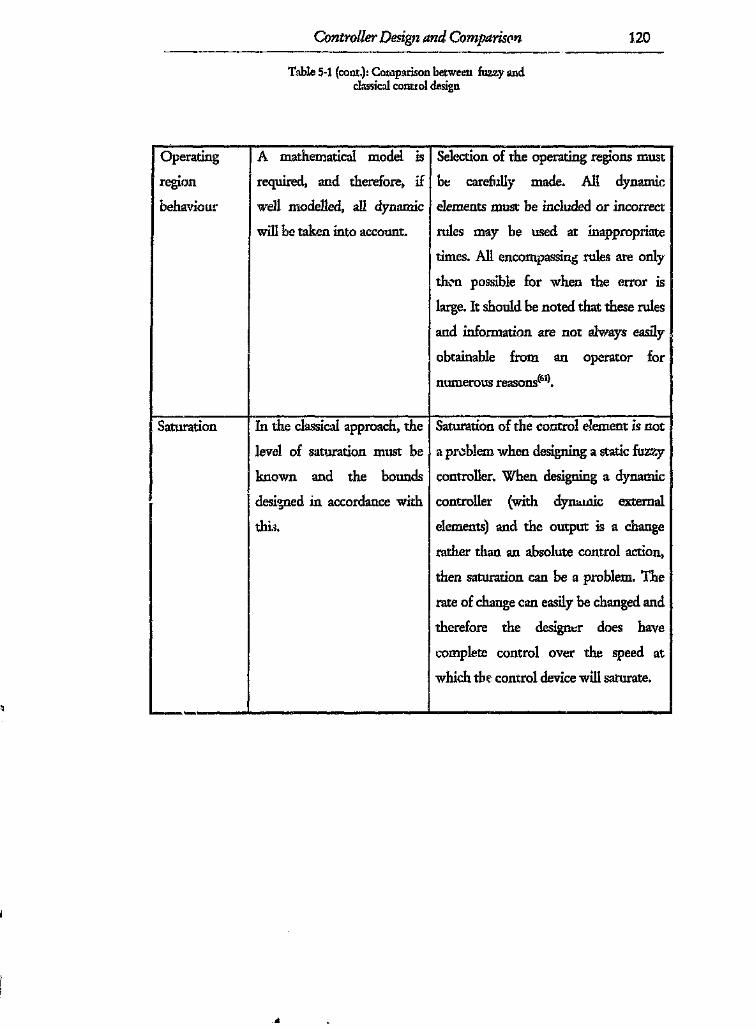
Controller Design and Comparison 120---.-~----
Operating
region
behaviour
Table 5·1 (cont.): Comparison between fuzzy andclassical control design
A mathematical model 1S Selection of the operating regions must
required, and therefore, if be carefully made. All dynamic
well modelled, all dynamic elements must be included or incorrect
will be taken into account. rules may be used at inappropriate
times. All encompassing rules are only
then possible for when the error is
large. It should be noted that these rules
and information are not always easily
obtainable from an operator for
numerous reasons(61).
Saturation In the classical approach, the Saturation of the control element is not
level of saturation must be a problem when designing a static fuzzy
known and the bounds controller. When designing a dynamic
designed in accordance with controller (with dynamic external
this, elements) and the output is a change
rather than an absolute control action,
then saturation can be a problem. The
rate of change can easily be changed and
therefore the designer does have
complete control over the speed at
which the control device will saturate.
~--------~------------------------------,----------------------~

Controller Design and Comparison 121
Stability
Table 5·1 (cout.): Comparison between fuzzy andclassical control design
Stability 111 linear classical Achieving a stable controller IS
control is well documented generally easy, but obtaining the desired
and the theory 1S well levels of performance is often difficult.
understood. II The servo motor illustrates this
problem, where the tracking bounds
Were veri hard to meet, but stability
was easily achieved. Designing to ensure
stability, without simulation, is difficult
and several methods have been
prop(l~ed(19.-IOft:>l).
Gain
Specification
Using a linear controller, the I-The fuzzy system offers the ability to
gains in certain regions of the specify gains at specific points in the
operating space cannot easily transient trajectory of the system.
be achieved and gam Therefore, if the Error/dError
scheduling is typically used. trajectory map is analysed, and portions
of slow movement are evident, the gain
111 that region can be increased.
Although this works well in theory,
achieving this level of proficiency
requires careful planning and
expenence.

Controller Design and Comparison 122
Table 5·1 (cont.) : Comparison betwee ,ul'...:..yandclassical control design
linearities
Plant non- The classical controller 18 The fuzzy system offers the ability to
typically linear and therefore cater for non-linearities in the system.
cannot cater for non- e.g. the tank system will empty and fill
linearities ill the same up at different rates. This effect can be
accounted for by changing the output
sets for opening and closing.
Noise --t-As discussed in section 3.2.3, If the gain around the o:")eratingpoint is
sensitivity T(s) must be kept small reduced. the fuzzy system can reduce
outside the control the system's sensitivity tc noise and
bandwidth to reduce the disturbance (e.g. use ?, windowing
effect of the noise. technique).
errors
information
Steady state The classical approach will .A typically designed fuzzy system will
have a steady state error., not allow for a steady state error unless
unless an integrator is used. the designer wishes one.
Design model A mathematical model IS Little mathematical model information
required for classical design. is required about some plants (but not
Qualitative knowledge is not all) for a controller to be designed.
easily incorporated. Qualitative operator knowledge IS
required. This IS illustrated by the
CSTR which was stabilised very easily.
The rules were obvious and simple. Yet
the control achieved was superior to the
classical with a fraction of the design
time.
IQFl' can bandit" aon-linearities through multiple linear plants,

Controller Design and Comparison 123
5.6 Advantages and disadvantages of fuzzy control
From the above comparisun the benefits of fuzzy control can be summarised as
follows:
• Fuzzy controllers can be highly non-linear. This means that the dosed loop
system can achieve performance unmatched by a linear classical controller.
1he interface to this non-linear control is easy to understand (i.e. rules) and
offers an intuitive method of implementing powerful control over a system.
• The non-linear nature means that the fuzzy controller is not bound by the
same restrictions that a linear controller is. This involves the inclusion of
plant non-linearities (e.g. saturation, slew rate) into the design as well as linear
performance restrictions (there is no response time! overshoot trade off).
• The ability to implement local control. Each area 01" the fuzzy control surface
can be optimised to suit the specific state that the plant is in. This differs from
the classical approach where one controller must suit all states (unless gain
scheduling is used).
• Ability to capture operator knowledge. This is possibly the greatest asset of
fuzzy control. Using classical control, only numerical knowledge can be used
in the design. With the fuzzy approach, qualitative kno: vledge can now be
included in the controller. This has implications when the qualitative
knowledge about a plant is comprehensive, but little is known quantitatively.
This qualitative knowledge has significant value in monetary terms, and a
method of using this could save significant design costs. There is no need to
pay large sums of money to develop a plant mathematical model, when a
qualitative one already exists.
• Noise suppression and disturbance rejection can be better handled. Fuzzy
controllers do not inherently reject noise better than the classical controller,

Controller Design and Comparison 124
but they do have the ability to. This is derived from their inherent non-linear
nature.
• Normally, when. a fuzzy controller is designed, it ensures that the system willnot have steady state error. This is in contrast to the classical problem where
high gain, or an integrator, is required.
• There are methods of using fuzzy logic systems to model a plant. Using the
inverse of this fuzzy model presents a method to apply control to the plant.
• Fuzzy controllers can implement complex objectives well. If a cost function
needs to be minimised or another supervisory approach is required, the fuzzy
controller is well suited. This is because supervisory objectives can easily be
reduced to a rule form. The higher the level of controller required, the more
complex the objectives become which increases the benefits which fuzzy
control has to offer.
.. High level adaptation of other controllers is possible. When control engineers
are designing a classical controller, they make choices based on their
knowledge of the plant. These choices can often be reduced to rule form
which can then be used to implement on-line changes to another controller.
The increased control performance comes from the ability to add more
information to the existing form of control.
• Adaptive fuzzy systems offer high robustness as they can change their
structure as the plant parameters change. This form of dynamic control
requires a very basic model ("\f the plant, while fine tuning can then be
performed while the plant is operating.
• The "fuzzy" nature of fuzzy control allows imprecise concepts and ideas to be
transformed into meaningful control actions which can be effectively used on
a plant. This is particularly important when the operator's knowledge is vague
and imprecise.

Controller Design and Comparison 125
• The control designer does not require detailed control theory to design a
workable fuzzy controller. This offers opportunities for less qualified
personnel to design controllers. The easy interface to the control concepts
provides a better situation for the operator to become involved in the desi~,~.
• The effect of external influences on a phnt are not always easily
mathematically definable. The fuzzy controller, using more sensors, can use
information about external influences to provide better control through the
use of more information which was ignored before.
The following disadvantages have been identified:
• There are very few analysis tools available. The biggest issue related to this is
the stability problem. Although methods have been proposed to address this
issue(40,39ct all, no overall solution has been found. This means that when a
controller is designed, the stability of the controller is always in question, as it
has not been proved stable for all states and inputs.
• No direct method of incorporating quantitative information is possible. As
illustrated by the servo motor where clearly defined tracking bounds are
present, the fuzzy controller cannot include these bounds in the design.
Repeated simulation is required to analyse the performance and ensure the\
closed loop system is within the specified bounds.
• Classical control is well defined and has a large body of theory and design
tools supporting it. Fuzzy control has no transparent design tools supporting
it and more work needs to be done to develop more design and analysis
techniques.
• The design process relies heavily on the designer to make choices regarding
certain aspects of the fuzzy controller (e.g. defuzzification method). The
number of choices are vast, with little understanding of the implications of
these choices.

\\
Ii
Contrc ller Desi[Tn and Comparison 126
• The design method is iterative and often time-consuming depending on the
plant being controlled. Classical control design methodologies offer
predictable controllers provided the modelling, non-linearity compensation
and design philosophy have been followed.
• Including frequency concepts in the "fuzzy" domain is difficult. The fuzzy
controller must be given the frequency information through a differentiator
or similar device. This is in contrast to the linear classical controller, .where
the frequency response of the syst ern can be well defined and information
regarding this domain easily included.
• Adaptive systems require a disturbance to be placed on a plant before the
adaptive system can make meaningful changes to the controller.
• If the fuzzy system is working well with one set of conditions, one cannot
infer that it will work with another set (e.g. although the step response may
be acceptable, the sine wave tracking response may not be).
• The system is far more complex than a simple transfer function controller.
This means that iml-l(:'K~ntation costs are usually higher, especially when
external dynamic elements are required.
• The quality of the final controller is largely dependant on the quality of the
designer. Two fuzzy control designers may come up with two controllers
which may both work within the specification bounds, but be very different.
The implication of this is that one controller may be more robust than the
other without quantifiable reasons. The classical control situation is different.
If the desired specificat.cn bounds are used in the QFT design process, the
controller obtained will resemble another controller designed by the same
process. The reason this is true is that the classical design technique (QF1)
quantifies the bounds such that the required controller. is one which meets
these bounds. The fuzzy control design techniques does not offer an easy

Controller Design and Comparison 127
method of including these bounds and hence the controller design level (under
or over designed) is not easily determined.
• There is no best controller in fuzzy control. As the design process is iterative,
the controller can always be improved upon, but the complexity increases as
does the design time.
,~ Fuzzy controllers are typically static systems. This means that external
dynamic elements may have to be added before effective control can be
obtained (e.g. an integrator or some form of storage element).
5.7 Summary
The design of the QFT classical controllers and the fuzzy controllers is very
different. Each uses the knowledge available in different ways and hence each has
benefits, based on the dominance of the nature of the technique and the
knowledge.
The fuzzy controller shows superior noise suppression and noise rejection in
most instances, which is due to the ability of the designer to scheduie non-linear
gains. The classical technique gives better control when the plant is hnear (servo
motor) or when fuzzy rules and sets are not easily obtainable. The CSTR
investigation demonstrates the power and possible future of fuzzy log.c control,
The combination of the two systems results in a powerful and robust controller.
This is achieved as it is now possible to combine both knowledge forms available
into a better controller.

Conclusion 128
6. Conclusion
Fuzzy control is a method of developing controllers for proct.sses by means of
multivalent linguistic information. The information which is used in the
controller design is thus not the same as that used in the classical control design. A
totally fair comparison is difficult for this very reason. That fuzzy control works!
is not disputed, but where it should be used needs to be qualified. 'The
investigation brought to light 3Qm"~ issues which are already known and
documented(lo,23,62.cr all, but new issues about the application of fuzzy control have
been discovered. The scope of this investigation was limited to pure fuzzy
systems, classical QFT systems and hybrid fuzzy/classical systems. Adaptive
fuzzy systems were not investigated! and this should be borne in mind when
reading the conclusions. The benefits of fuzzy control can be derived from two
characteristics of fuzzy systems, namely their non-linear nature and their ability
to capture multivalent linguistic information".
It should be noted that a fuzzy controller can always provide better control than a
linear classical controller, due to its non-linear nature. The development time,
cost and complexity all need to be included when comparing the systems.
The myth that fuzzy systems, "fuzzify", cloud and hide information is not true.
What it does is represent this knowledge 1n a different manner, which is often
more meaningful than bivalent mathematical knowledge.
Another myth is that fuzzy systems are more robust. While they have the ability
to be more robust through localised non-linear control, they are not inherently
I This would require a comparison between adaptive fuzzy control and adaptive classical control.
2 This has many consequences including the fact that the controller can use human rationale for its designmaking.

Conclusion 129
more robust. This advantage should be further investigated such that it can be
effectively used and clearly understood.
Fuzzy control caters for vague linguistic information. It results in a static non-
linear gain controller. This is an advantage at present due to the inadequate non-
linear classical control design tools. If such a tool were developed, the main
advantage of fuzzy control will be its ability to capture linguistic information.
Both classical control techniques and fuzzy control design techniques use
knowledge of the plant in the design, but in different forms. Classical control uses
a mathematical model, while fuzzy control uses a linguistic model.
From the literature reviewed ill Chapter 3 and the comparison detailed in
Chapter 5, it is suggested that fuzzy controllers offer the greatest benefits in the
following areas:
• If the process cannot be mathematically modelled either due to complexity
time or cost, then fuzzy control should obviously be used.
• When there is a large amount of qualitative knowledge about the plant
through vast operator experience, it is much cheaper to convert this into a
fuzzy controller than to develop mathematical models for use in classical
control.
• When the objectives are complex and require some form of human
"intelligence", fuzzy control can include this "intelligence" through rules.
• In a hybrid system where both operator knowledge and mathematical
knowledge can be combined into a system which will utilise them effc( ively.
• If the system dynamics are well defined, but highly non-linear, the fuzzy
controller ca . be easier and quicker to design than multiple linear controllers
to deal with the non-lmearity.

Conclusion 130.-----. ~.----
• If the performance bounds cannot be met with a linear controller, due to the
properties of linear controllers, then a non-linear fuzzy controller can be used
to achieve these bounds, but at the cost of an increased design time and high
complexity.
• When the system characteristics (e.g. non-mirumurn phase) make linear
control difficult.
• ITnoise or disturbances are problematic, fuzzy control can be used to reduce
the effect through careful design using its ability to implement localised
control.
• Automation of high-level objectives or when the objectives can be better
explained through rules rathe, chan mathematical formulas.
IT a classical controller is working well, there is 110 reason why it should be
changed. However, if the classical controller is not achieving satisfactory results,
then the fuzzy controller can offer methods of improving control through the
inclusion of more knowledge into the system. Many issues need to be addressed
before fuzzy control will be accepted as an addition to or replacement of classical
control. The question of stability, inclusion of numerical knowledge and various
aspects which have been discussed in Chapter 5 need tc be addressed. At present
fuzzy and classical control shoul-l be seen to be complementary. Each shows
significant power when used exclusively in their own domains', but when used in
regions ~ here their domains overlap, the better controller depends on the
situation. The type of specification bounds must be taken into account when
determining the type of control required. (e.g. the fuzzy controlled servo motor
could not track the sine wave but showed excellent results on the step test).
I The classical domain is totally quantitative with clearly defined models and bounds. The fuzzy domain canbe seen as a combination of both qualitative and quantitative information, but its ability to include thequantitative knowledge is limited.

Conclusion 131
When a full mathematical model (relatively linear) of the system is already
available then classical control will be sufficient (provided the requirements can be
met with a linear controller). If a mathematical model is incomplete or lacking, or
the dynamics are highly non-linear then the system will be better controlled with
a fuzzy controller. The complexity of the system and the objectives must be
borne in mind when choosing the form of control to be used,
6.1 Future research
There is a vast amount of research which needs to be done in the area of fuzzy
control. Two main areas can be identified:
• Design and analysis tools ; One of the major problems with fuzzy control is
the lack of cools for incorporating knowledge into the design and analysis of
the final design. The major problem is the issue of stability, How should
stability in terms of a fuzzy control system be defined ) How can one define
robust stability (stability margins) in the area of fuzzy control ? A method of
determining stability regardless of the type of system is required. This could
possibly be obtained from a combination of the plant and controller map
surface. The inclusion of tracking bounds and other bounds (noise, input
disturbance, output disturbance) need to be addressed.
• Quantification of the effects cf design options : The design of a fuzzy
controller involves numerous choices regarding the number and shape of
membership functions, fuzzification, defuzzificarion and various other aspects.
The effect of choosing one method over another is poorly understood. What
needs to be investigated and quantified is the effect each choice has 011 the
overall system, and therefore a method of quantifying robustness, noise

Conclusion 132
suppression, disturbance rejection and uncertainty must be incorporated into
the design.
Another area which needs investigation is the conversion from fuzzy model to
numerical model and vice versa. If a good method can be obtained to achieve this,
then both qualitative and quantitative knowledge can be used in the model and
controller design.

Appendix A: Model Parameters 133-----~----.
Appendix A :Model parametersA.I Servo motor
Table A.l : Model parameters for servo motor
Parameter Value Unit
KT 4.382 x 10⁻² Nm/A
Kb 39.4 x 10⁻³ ~ 48.2 X 10⁻³ V/(rad/s}
Jrnotor 29.57 x 10.(,~ 47.88 x 10⁻⁶ Nm.i
Bmotor 92.41 X 10⁻⁶ -"7184.15 X 10-6 Nsn.s/rad
Rm 0.8 Q
Lm 1.2 mH
-A,2 CSTR
Table A.2 : Model parameter values for CSTR
Parameter Meaning Value Units
M-Reactant
Fl flow rate of Minto 3.60789 moles.s"tank
XMF mole fraction of M in .002feed stream

i\
Appendix A: Model Parameters 134
LlHFM heat of formation of -640 kj.mole"M
CPM specific heat capacity 32.00 J 1 -loCI.moe.ofM
PM density ofM 555u6 moles.m?
Tl temperature of feed 18 °C ,
stream FI
N·Reactant
F2 flow rate of N into 3.60789 moles.s"tank
XNF mole fraction of N in 0.08feed stream
~FN heat of formation of -740 kj.mole?N
1----CPN specific heat capacity 29 J.mole", °CI
ofN
PN densityofN 55506 rnoles.m"
T2 temperature of feed 18 °Cstream F2
Inert
LlHFr heat of formation of -571.68 kj.mole'inert, I
CPl specific heat capacity 75.4 J.mole", °C:tof!
PI density of i 55506 moles.m?
Product
AHFl' heat of formation of -2400 j.mole"
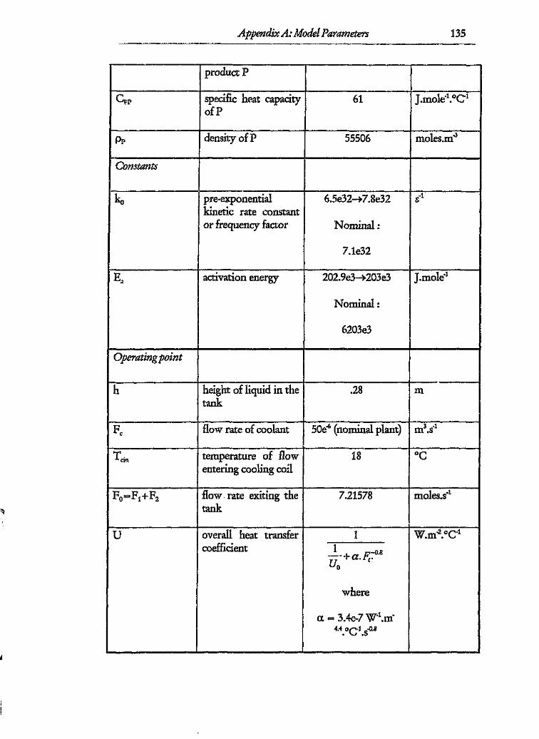
Appendix A: Model Parameters 135
I product P
Cpp specific heat capacity 61 J.mole-1.oG1
ofP
r--'pp density ofP 55506 moles.m"
Constants
k pre-exponential 6.5e32-+7.8e32 -10 s
kinetic rate constantor frequency factor Nominal :
7.1e32
Ea activation energy 202.ge3-+ 203e3 j.mole?
Nominal :
6203e3
Operating point
h height of liquid in the .28 mtank
Fe flow rate of coolant 50e-6 (nominal plant) m3.s-1
Tcill temperature of flow 18 °Centering cooling coil
Fo=F1+Fz flow rate exiting the 7.21578 rnoles.s"tank
U overall heat transfer 1 W.m-2.oGtcoefficient 1-- +a.p;:o,su,
where
a. = 3.4e-7 W-t.m-4.4.°Cl.SoO,8

[
Appendix A: Model Parameters 136
-~- Uo~3000w.n?:"G' ]
A.3 Tank
Table A.3 :Model parameter values for tank system
Parameter Meaning Value Units
r radius of tank 1 111
h height of tank 2 m
ho initial height of tank 1.5 m
(nominal)
p density of fluid 1 kg.m"
K valve coefficient 0.0669

Appendix B: Block Diagrams
Appendix B : Block Diagrams
These diagrams are extracted from Simulink under J\1ATLAB~.
B.1 Servo motor
Summary: Selection of the method of control and the existence of noise must be
made before simulation. These button control flags which are used by
the system. There is a dedicated plotting program which is opened by
clicking on the plotter button. The method of integration used for all
simulations is Linsim with a maximum step size of O.ls.
Methc.:2Of Contrciupeh Plottet :::J Positional Servomotor Control Setup
bySIJ/'l'm:m:1:JIUU: 1996
, UF J CONtroller iI, fuzzy Conttbl:=J
Seit'ct.NuiSf! OnfCff
C NONOI5i! JMdllRli:r=:J
:e6G!...
Send time to workspace
~Cicek Tim.
Add Noisa
Figure B.l: Servo motor main block diagram
137

Appendix B: Block Diagrams 138
.----~s
--_...~O",putlnHad/s
Model of ~enlOmo~cr
TIli5 Is n model cf1he servUrTI{ltor 'Jthi",'l bke"en inllut voltag~("'fi12't" and outputs In
radis.
Figure B.2: "Servo motor" subsystem
Figure B.3 : "Controllers" subsystem
~--------------~~
Figure B.4: "Noise" subsystem

Appendix B: Block Diagrams 139-,---~-.--~---~----- --~-,---------.----
B.2 CSTR
Summary: The cs~ must be initialised (constants and state variables loaded)
and the means of control and presence of noise and disturbances need to be
chosen. The relevant code is given in Appendix D. The integration method used
is Runge-Kutta 5 with a maximum step size of 1s.
Click To Plot Resut!s CSTR SIMULA TORby S.D. Florence
June 1996
Ciia BefCire SifOOfaUon
I InitialiseCS1!:J
Submenu For Pallli Variatlen
r Add?ann·"!:::JSeleU Noise Select tnsturtence C:'T=1I rlul"'~ I !lI=:e~dc::::::J Ili~.0" ~
[SCfPCUilJI---~ Controllers ~LI ~,~"" ~-E?-r1- . [Scn~r NO~S~" Sele~tControl
;.~:z/:laFigure B.S : Main CSTR System.
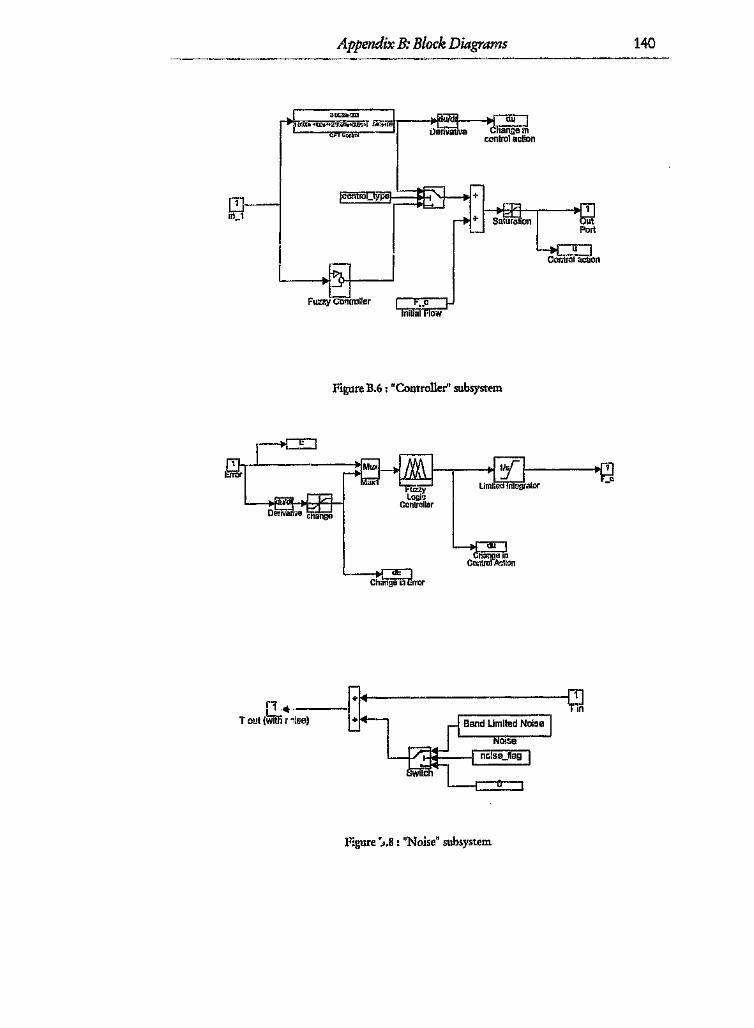
Appendix B: Block Diagrams
[2]_..iO_1
4----'Fuzzy Controller r--..."""-"
Figure B.6: "Controller" subsystem
~rt:_Denvat\"eW
~i3~Control k.:lion
c~lng;~n~rror
r'~ ~ ..11 ... _
Tout(Willi r1ise) + YBand limited'NO~J L. NOise
----~-----------~
Figure ·.>.8: "Noise" subsystem
140

m.-1=t===~~I---.---'-+-----f'i'IT Conlnbutons to
Chan~y~ ~1thalpy
F10
1r1f'F3[f.J1
FIO,);T: F2
I
Appendix B: Block Diagrams 141
Figure B.9 : "Hand Limited Noise" subsystem
l
..+
Fl' 2
Figure B.10: "CSTR" subsystem

Appendix B: Block Diagrams--~-------------------
142
~}---------+----------Temp8ratutu
m1f-uXm-Xm
~-------------~~Figure B.ll : "Mass balance equations" subsystem
kO'co'V'u
Figure B.ll; "Rare of reaction" subsystem
Figure B.13 : "Block Ill" subsystem

Appendix B: Block Diagrams~---- ---------------
143
~I+----l
~ruQ} +ConslZnt
Figure B.14 : "Block IV & V" subsystem
(U(3)'Ac'u(2)+ Tel'(u(1 )'looo'4100-u(3)' AcI2»lluil)'IOOO'4 '186+u(3)'AcJ2)
co
Figure B.1S :"q" subsystem
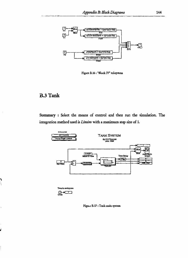
Appendix B: Block Diagrams 144
Figure B.16: "Block IV II subsystem
B.3 Tank
Summary : Select the means of control and then run the simulation. The
integration method used is Linsim with a maximum step size of 1.
Ce!JC\CJ(i.trc.1
TANK SYSTEMBy SD.Florence
June 1996
G~Crock
Figu.e B.17: Tank main system

Appendix B: Blade Diagrams 145
..rncOI;t!crAction
Oulilut
Figure B.iS ; "Controller" subsystem
Figure B.19 : "Tank" subsystem

Appendix B: Block Diagrams 146-~---~----------------------------
B.4 Nonminimum phase plant
Summary: The integration method used is Rtmge-Kutta 5 with a step size of 10.
Nonminimum Phase PlantBy S.D.Florence
June 1996
-~- s- MUle ESa(s+3)(s+4)
ani .ux I Auto-~caleGraph
~a~
Time to workspace
~Clock t
Figure B.20 : Nonminimum phase plant system

Appendix B: Block Diagrams 147
B.5 First order system with dead time
Summary: The set point .isa series of steps. The nominal set point is the value of
the normal operating set point before a step is imposed on it. Tuning is only
performed on the "up" portion of the step.
C9-+C!:JClock
L_
First Order System with Dead Time{3y S.O,FIIJ"",(;e
June 1996
Normal F•• dback
Feedback Etror Em
U'~[0\. 'gn
NOMinm-setPClint
Figure B.21 : First order system with dead time

Appcn,.{ix C: Controllers 148------.~----~.-
Appendix C: Controllers
This section summarises all the controllers used in the investigation.
C.l QFT controllers
C.l.1 Servo motor
Ccntroller :
The Nichols plot is given below.
I!O
&J
.~ ~5a ·200X "","(itgtIe) Y 1IogniI""'ldB)
·100
Figure C.l : Nichols plot of servomotor controller

Appendix Co Controllers
C.1.2 CSTR
Controller:
O(S) = 0.001789 (' s )'(s 1132i + 1 b.631 + 1)
The Nichols plot of the plant, with the controller is:
20
(_:_ - -, 1- - -_.
i... I
.... - ,---·~o
~Q
.il)
-<C
,100
.1!-U
·35IJ
f - - - t- -I
- - - - -t -"
,300 .2[ij ·100
~pt""'(iI<!IIt")V:~-"'(<!!Ii·100
Figure C.2 ; Nichols plot of CSTR controller
149

Appendix C: Controllers 150
C.l.3 Tank
Controller:
s---+1G(s) == 0.03115 0.0229
s( 10~~0+ 1)
The Nichols plot for the system is :
l_I
. .l _ .__I
·ID
·Zl
.'iJ
.:;:j) ·lSl
Figure C.3 : Nichols plot of tank controller

Appendix C: Controllers 151
C.2 Fuzzy controllers
The designed fuzzy controllers are given in this section. For each controller, the
choices made, rules and control surface are given. The exact membership
functions for each controller have not been included.
Table C.l summarises the symbols used in the rule base.
Table C.l : Fuzzy set symbols
-Symbol Meaning
NL Negative large
NM Negative medium
NS Negative small
N Negative
Z Zero
P Positive
PS Positive small
PM Positive medium
PL Positive large
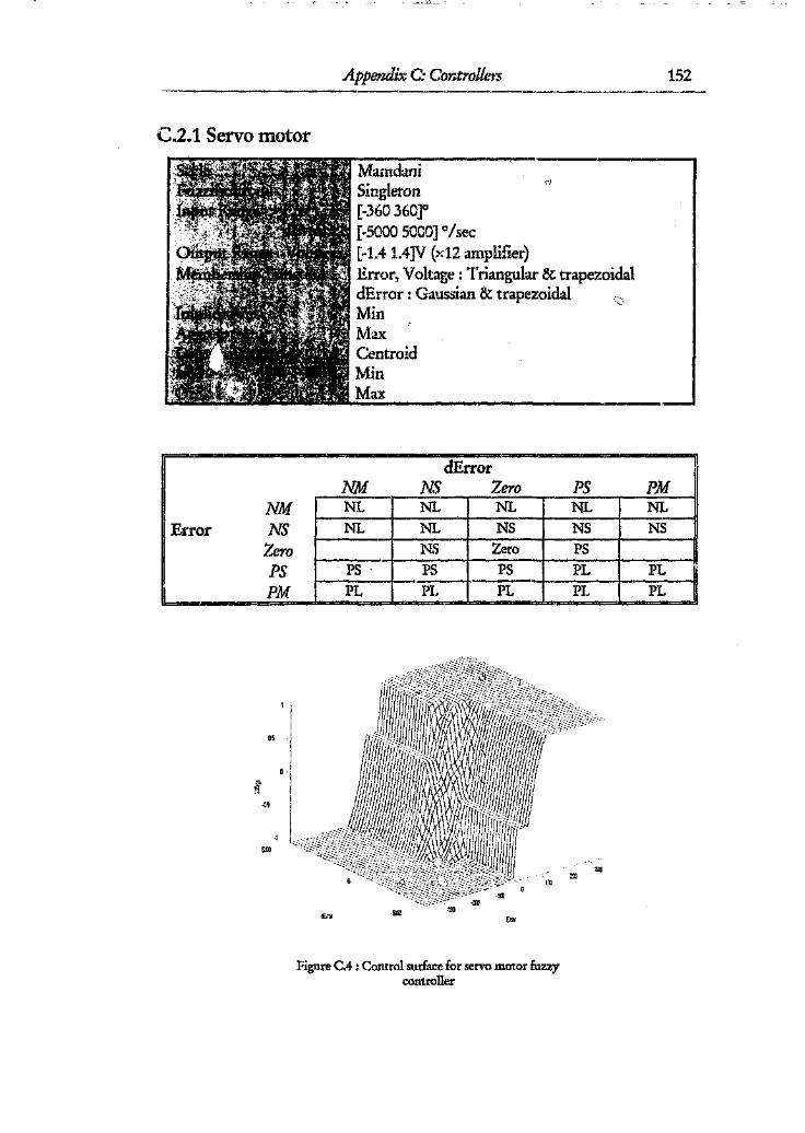
Appendix C' Controllers 152
C.2.1 Servo motor
MamdaniSingleton[-360360]°[-5000 5000] a/sec[-1.4 l.4]V (>d2 amplifier)Error, Voltage: Triangular & trapezoidaldError : Gaussian & trapezoidalMin
-,_,
MaxCentroid:MinMax
I- =1dError
NM NS Zero PS PMNM NL NL NL • NL NL
IError NS l'TL NL NS NS NSZero NS Zero PS
I PS PS PS PS PL PL,,- -II PM PL PL PL PL PL
UI
"~~5
.-00
Figure C.4 : Control surface for servo motor fuzzycontroller

Appendix Co Controllers
r::.2.2 CSTR
.====.:=0:...
dErrorN Zero P
LW dose fast close fast close fast
NS close fast dose slow I close slow
ero close slow no change open slowf.-.
PS open slow open slow open fast
~ open fast open fast open fast
cs
o
Figure C.5 : Control surface for CSTR fuzzycontroller
153
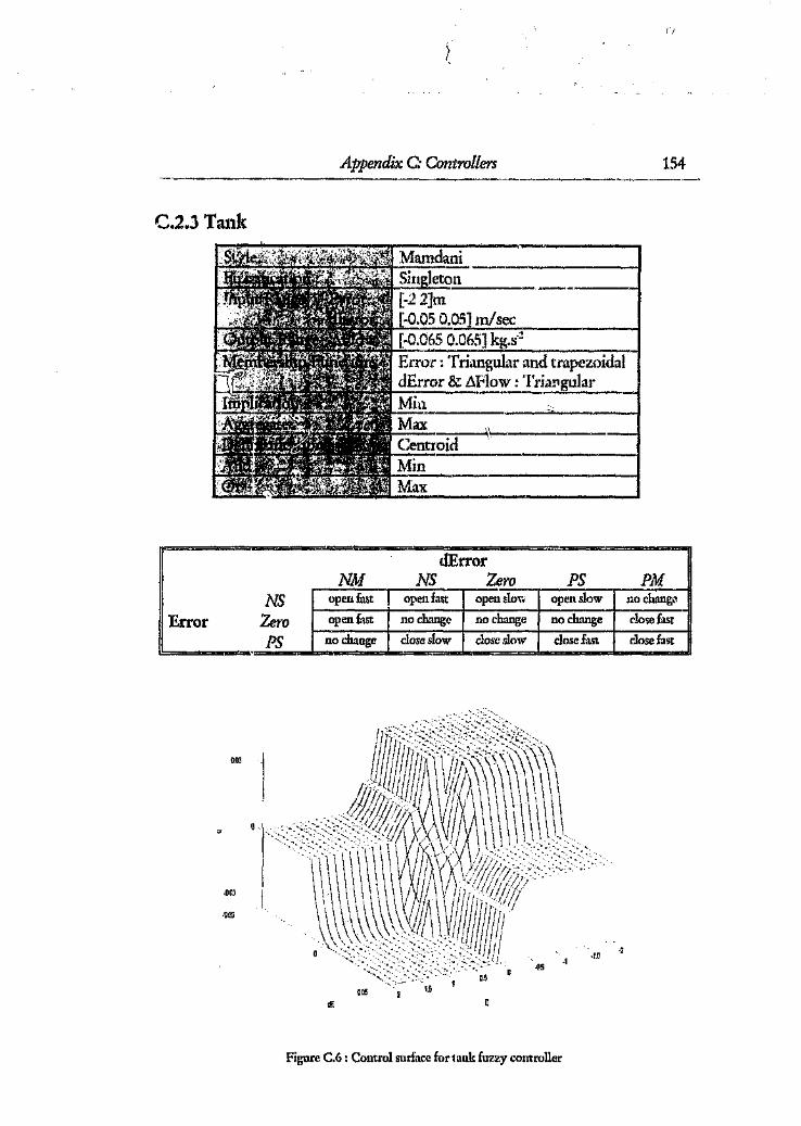
C.2.J Tank
(,I
Appendix C: Controllers 154
Error
l'======~'
om
- - - --dError
NM NS Zero PS PMNS openfast open fast open sloe open slow no change
Zero open fast 110 change no change no change close fast
PS no change dose slow close slow dose fast clo~cfast . ij
.Hi ·2
0.05 15
Figure C.G : Control surface for tank fuzzy controller
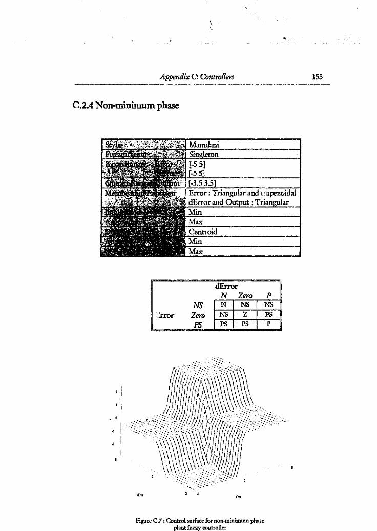
Appendix C: Controllers--_._-----_-
C.2.4 Non-minimum phase
dError7N zero P
NS N NS NS
ero NS Z PS
PS .....J_ps PS i)'".
·2
·5
Figure C.; : Control surface for non-minimum phasetaut fuzz controller
155

Appendix C: Controllers
C.3 Hybrid Controller
<:.3.1 <:lassical
Controller:
38.42G(s) :::: 1 ? 0.4053
100.62 s: + 2 -100.6 s + 1
Nichols chart (no dead time):
.10
.2')
.J(J
-10
.:;0
.QJ
.70
.3;"
.-t--I
.3i!iJ ·2m ·,00X:1'ha1ll(i(-;"b) y v,agrAt!I.(ctu)
·150
Fi~re C.8 : Nichols plot for hybrid ~mith predictorcontroller (QFT section)
156

\I'-
J(
Appendix C: Crmtrollers 157
C.3.2 Fuzzy
1- '""' . ==r
P hatNM NS Zero PS PM
NM z Z Z Z zNS Z Z Z Z Z
P Zero Z Z Z PS PMPS Z Z NS Z z
I PM z z NM Z Z
DB
04
Figure C.9 : Control surface for hybrid Smithpredictor controller (fuzzy section)

Appendix D: Mit TLAB* Code 158,-_--------
Appendix D :MATLAB® Code
This section includes the significant MATLAB" code which was written for this
investigation.
Note: Only code for the servo motor and CSTR is gIven. All other code
generated is not included as it is derived closely from the given code. Some
of the code given works ill conjunction with the Simulink models given in
Appendix B,
D.l Servo motor
D.1.1 servo tf.m
(~************~**************~*************,,*** servomocor o posit.ionnl Centrol .**~l **********************~******************
n. Linear Model G"merator
" Prepared by S.D.Florence
" First Edit : october 1995
Last Edit : June 19%
" Calculates the transfer function of the servo motor
Inputs : NOlle
':' Outputs : transfer funct.ion : n, d
zeros, poles and gain: z,p,k
format compact;
'.',Kt : 'I'orqup Constant [4. 382<;>-2J
I:t. ~" (\. 382e-2i
~ Rb : Back EMFConstant [39.4e-3 48.2e-3]

Appendix D: j11ATLAB2 Code___________ o __ ~ _
fill ~ 39.4e-3;
':;i(b ,~ 48.2e-3;
"Ra Armature Resistance [0.13 1.2]
Ra 0.8;
J Noment of Inertia [29.578-6 47.88e-6)
.J ~ 29. 57e-6;\iJ : ,17.88e-6;
OJ T,a Armature Inductance [1. 2e-3]
La 1.2e-3;
B Rotational Friction [92.41e-6 184.15e-6J
B "" 92.41e-6;'liB = 184.15e-6
'0- Servo AmplifieI:
Ea 1;
o. Tra.1sfer Function
n ~ [\Kt/ (J*La) iJ;
d [1 (B/J+Ra/La) «Ra*B) / (I.a*J) + (I(t*Kb) / (La*J» OJ;
[z,p,kl~tf2zp(n,d);
D.1.2 ptnap_s.m
<' ********************" *** Plot ur Men.u ***
.~ ********************
" Prepared by S.D.Flor;"nceFirst Edit November 1995
Last l':tiit ,June 1996
" Prepares and plots the S8t-VO motor gr.a hs
159

Appendix D: MA TLAB~ Code
For use IVith the Simu,link model
"Inputs op_no (from simulink)
.. ouputs Graphics
g:i:id_on 1;
hold on 0;
if op__no 1
figNumber ~ 1;
figNurr~er~figure( ...
'Name', 'Data Plotting', ...
'NumberTitle', 'orf', .••
'Uni ts' , "nozma l i.aed ' , ...
'Position', [0.10 0.45 0.65 0.45J);
0P._no = 2;
end;
if op_no .,<.
h '" uimenu (figNumber, 'Label', '",,!neral');
uimenu(h, 'Label', 'Toggle Zoom', •• ,
'Callback', 'op_no=100;pmap_s');
h = uimenu(figNumber, 'Label', 'Plant');
uimenu(h, 'Label','Plot Tracking Position', •.•
'Ca]'lback', 'op_Ilo"'3; pmap_s;');
tlimenu(h, 'Label', 'Plot Velocity (Ract/5) ', •.•
'Separator', 'on', .••
'Callback' , 'QP__1'J.o=!J;pmap_s;');
ui',16nu (h, 'Label' , 'Plot Vel.ocity (PPM)', •••
'Callback' , 'op_Ilo=5; pmap._s;' J;
h ~ uimenu(figNumber, 'Label', 'Controller');
uamonu (h , 'X,abel' , 'Plot Cont: 'J1 Action', ..•
'Callbacl;' , 'op_no"'10; pmap_s; t) ;
uimenu(h, 'Label', 'Plot Error', ••.
'Separator', 'on', •.•
'callback', 'op_no"'11; pmap_.s; I"
uimenu(h, 'Labe).', 'Effect of Pre-Filter', .•.
'Callback', 'op_uooo12; pmap_s;');
h .~ uimenu (figNwuber, ':Label' , 'Fuzzy Aspects' J ;
uiraenu (h, 'Lahel' , 'Plot Hap Trajl,ctol'Y', •.•
'Callbacl:', 'op'_no~15; pmap_.s;' J;
160

Appendix D: .ArIATLAB· Code 161
h = uimenu(figNurnber, 'Label', 'Noise');uimenu(h, 'Label', 'Plot KOlse', ..•Callback', 'op_l'o",l':;;pmap__s;');
uimenu(h, 'Label', 'Plot Distribution', ..•'Callback', 'op_no~17; pmap__s;');
end;
if up_no 100
ZOOffii
end;
if op_no 101
hold_pn -(hold_on);
end;
if op_no 3
if hold_on == 0, cIa;else hold on, end;plot(t,r,'w',t,theta, 'r');ti tle ('Tracking Of Servomotor')
l:] abel ('Time (s)');
ylabel('Degrees');if grid_on ="' 1, grid, end;
end;
if op_no 4
if l101d._on "'= 0, cIa;else hold on, end;plot(t,w);title ('Velocity')>:label ('Time (s) ');ylabel('Rad/s');if grid_on == I, grid, end;
ondr
if cp_no 5

Appendix D: MATLAB~ Code 162
if hold_on =~ 0, cIa;else hold on, end;plot (t,60*11/ (2*pi) );title ('Velocit.:,")xlabel('Time (5) ');
ylabel ('RPH' ) ;
if grid__on == I, grid, end;
end;
if OP_110 10
if hold_on == 0, cIa;else hold on, end;plot(t,u);title ('Control Action')xl ebe l (''rime (s)');
ylabel('Normalised Control');if grid_on == 1, grid, end;
end;
if op_no 11
if hold_on == 0, cIa;else hold on, end;plot(t,r-theta);tit:e('Error Signal')::label('Time (~;)');ylabel('Degrees');if grid_on == 1, grid, end;
end;
if op_no 12
if hold_on == 0, cIa;else hold on, end;plot(t/r/'l~' ,t,r_dash, 'r'll
ti tJ.e ( I Effect of Pre-Filter - Before and After')xlabel ('Time (5)');
ylabel('Deqrees');jf grid_on == 1, 9rid, end;
end;

Appendix D: MATLAB· Code
if 0p_.no 15
if hold_on ~~ 0, cla;else hold on, end;plot (,,*60/ (2*pi), (r-theta], 'r');
hold on;number = ronnd(linspace(l,length(t) ,10»:
112 = u(number);
theta2 = theta (nwnbal');
r2 ~ r (nurnbez) ;
plot (1'12*60/ (2*pi), [r2-theta2], '\'10');
ti tIe ( 'r·!ovement in Hap')
,;label(,RPW ) ;
ylabel (,Error' ) ;
if grid __on ~= 1, grid, end;
hold off;axis{[-2500 ~~OO -360 360JI;
end;
if op_no 16
if hold_on == 0, cIa;else hold on, end;
subplot (211);
plot{t,n);
grid
subplot(212);
tJ.tle{'Nrise - Unfiltered')
::labelC"rime CS)');
ylabeI{'Pegrees');
plot (t, n_filt) ;
grid;
ti tle C'Noise - Filtered')
xl abe.l ('Time (s»');
ylabel('Degrees');end;
if op_no 17
if hold_on =~ 0, cIa;else hold on, end;subplot (211);
hist (n);
title('Noise - Ur,£ilteT.ed')
subplot(21<:);
163

Appendix D: M4TLABO Code
hist (n_filt) ;title('Noise - Filtered')
cndr
D.l.3 qft_serv.~n
~ ***************~*************\j *** Servomotor QFT Design ***" ***** of.-**·k***** ***************
Prepared By S.D.FlorenceFirst Edit : July 1995
" Last Edit : June 1996
" QFT deSign for servo mrtor
" Inputs : None':i Outputs : Graphics, and variables as selected
elc;clear;format compact;
" Assumptions made
model valid to 50Hz i.e. second order sufficient
******~**************~**********************************Part r :PROBLEH DATA
computing the boundary of plant templatesdisp ('Computing plant templates (20 plants at 8 fl::equencies)•..• ")dravmoH
G ~ 1; 613; b 3.1e4;
for k [7.6e5,1.2e6}*180/pl,nump(c,:) ~ k; denp(c,:) [1,a/b,O]; c c + 1:
end
164

Apperulix D: MATLAB~ Code
a = 673;
Zox: k ~ ['1.6e5,1.2('6]*15:l/pi,
nump(c,:) = It; denj;:(c,:) [l,a,b,Ol;cend
a - 613; b = 6.4e4:for 1: [7.6e5,1.2e6]"1o'0/pi,
nump(c,:) = k; denp(c,:) [1,a,b,O]; cend
a = 373; b ~ 6.~e4:for k = [7.6e5,1.2e6]*180/pi,
nump(c,:) = ]:; denp{c,:) [l,a,b.O];cend
a = 613; b = 5e4;for k = [7.6e5,l.2e6]*lBO/pi,
nump(c,:) = k: denp(c,:) [1,a,b,O];cend
\'; Compute responses
w = [.01, .1,1,6,10,20,lDO,le3.1e5]*~*pi;
Wb=[.1,6,lO,le3]*2*pi;P=freqcp (nump,denp, VI) ;
disp(' .)
disp ('plctt:npl (H, 11b,P); ':.shol'l templates')
dr awnow
plottmpl (t'l, wb,?). tale (. Plant 'l'emplates ') ;
qpause;close(gci);
~ *****************************+'********* '*******
':; Part II:
'2; BOUNDS
disp(' .)disp('Computing bounds ••• ·)disp( 1 .)
disp ( I bdbI=si.nobnda(1, \'1, vt, 1<1, P, rn; ':,u.arginsI ) ;
<lra~mOl'I
c + 1;
c + 1;
c + 1;
c + 1;
n, W in Hertz
165

Appendix D: MA TLABQ Code 166
" *** Robust r·jarqin t'leight *.;._,*
H c' 0; define radius
hdb.l=a i.sobnds (1,1'1,\-1b,I'll, P, Rl;
di,sp i 'p.lotbnds (bdbl), ',ishm-l bounds');
plotbnds (bdbl) ,title ('Robust ~lilrgins Bounds');
qpause;cl.Jso(qcf);
o~"* * Tracl:ing Bounds "X * *
d iap t ' ')
disp ('bdb7~sisobnds (7, vs,Hbd7,WI, P); ~;tracl:ing bounds');
dr ill'mOI'1
':, • * * Upper Bound * * *
Im_u .c. 150;
nil wn,_uA2;
du [1 2*zota_u*11H u Im~uA2l;
mll~£reqcp (nu,du, ~1);
" *** LO\-1crBound ***
1'111_1 ,- 100;
zeta. 1 O. 8~);
ul \'/ll_1"2;
dl (1 2*~:'.!t:i! l"I-ln 1 \'m_l"'2];
ml~freqcp(nl,dl,w);
v17~·[abs (ron); abe(ml) J; '," t racki.nq Heightbdb7'~sisobnds (7, \'I, ~;bd7, 1:17, P) ;
rlisp ( ' plotbnds (bdb'l); ':,shoNboundsr);
plotbncis(bdb7),Litle('l\obust Tl:acking Bounds');q!)dUDo;clOSf;(gcf) ;
clillP (' ')

Appendix D: At.1ATLI1B$ Code
dl ap ( 'bdb~gIpbnds (bOOl,tdb 7); ~,gl:ouping bounds')
dr"I'mm'j
bdb"'gr:pbnds(bdbl,bdb7);disp ('plotbnds (boo); ':;ShON all bounds')
plotbnds (bdb) , ti tle ('1,largio:> and Tracking Bounds');
qpause;close(gcf);
<> Intersection Of Bounds
disp(' ')di sp (' ubdb=aoct.bnda (bdb); ':;intersect bounds')
dell'mm'!
ubdb~sectbnds(bdb);disT' (' plotbnd~ (ubOO); 'i.sho\') bounds')
dr aunow
plotbnds(ubdb),title('Intersection of Bounds');
qpausor close (qcf') ;
o **************~********************.*******************',; Part UI:
n. DESIGN
(lisp,' ')
disp t ' Deslgn' )'.li,sp ('lpshape (vll,ubdt, nLD,dLO,delO,ncll,dcO); 'Hoop shaping')
crrawnownompt~l; nLO"·numpmompt , :); dLO~denp (nompt, :); o, nomina]. plant
del()~,O;
vrl=Loqspace (-2. ~, 200) ;
neU 0 2.310Je-003 2.9500e-OOl];deO 12.19128-008 2.0278e-004 1.0000e+000J;Ipsha.pe (I'll, ubdb, nLO, dLO,<lelO, ncO, deO); ':,qpnuse;numu=ncur donc=dcur
G"'lJ::eqcp (numc, done, N) ;
di.ap (' ')
disp ('pfshape ('I, \'),1'lbd7,vl7, P, [1, G, 1, rlfO, ctfO); ;~pre-filter shilpinq')
dr awnovr
pf.'lnLlpe(7,11,\'lbd"l,I'J'i,P, (],G,l,l1f(',dfO); qpauser
numFc'l"lfO; <teuF,·dfO;
167

Appendix D: .lhATLAB' Code
" Part IV:
c ANALYSIS
disp t ' ')
d.isp ( 'llnalysis .••. ' )
p~fn'qcp (nump, denp, 111);
G~freqcp(numC,dE~nC,wl) ;
F~"fr:eqcp (numF, denb', I'll);
di.sp t ' ')
disp ( ' chks i.so (1, ~/l, wi , P, R, G); ";marg:l.ns spec')
dral-ffio\1
ch);s.!.so(l,I·/l,vll,P,R,G) ;
qp2.use; close (gc:f) ;
disp(' '};
disp('chJ;silJ"(7,1~1,vn,p,R,G, [l,P); "ltracking spec')
dravmov/
Lnd=f Lnd(1~1<~~15);
mu= [ J; mf= 1]; \17'" [ ] ;
mu"'freqcp(800. [1 40 80C],t'l1);
ml~fJ:l:oqcp(2, [1 2),I'il);
vl7'" labs (nu) ; abs (rru ) ]; 'Ci t ruckanq w-,ight
chksi so (7, I'll (ind), 117(:, ind), p (:, ind), n, G(Lnd}, [J, F(ind);
qpause:close(gcf);
D.2 CSTR
D.2.1 c curve.m
******l****************************************W***~.**Characteristic Curve of CSTR t10del
~ ************+*~*********k******************************
" c'l'ep"I.L! by S. D. Florene,;
" Fil',t Edit: October. 1995" Las t Ldi~ : Febr.uat'y 1996
" Genel'atl~s the chdractel'i5tic curve fur ,I CS'l'R
168

Appendix D: M11LAB~ Code
" Inputs : NoneOutputs : Graphics
clear;
':, *** [·1Flot'1 ***dHfm ~ -640e3; J.mole(-l)Cpm C~ 32.00; ':; J.moll,(-l).deg K(-ll
rO_ln ~ 55506; mole.m(-3)
Tl 18; ~ deg(C)ITl 3.60789;
Xmf = 0.002;
~, *** N FIoH ***dHfn ,~ -740e3; e. ,T.mole(-l)
Cpn '" 29.00; ',',J.mole{-l).deg 1\1-1)
rO._n ~ 55506; ':, mole.m{-3)T2 18; ';, deg(C)F2 3.60789;
Xnf = 0.08;
~ *** InGrts ***dHfi = -571.6883; \i J.mo!e(-l)Cp:i ,~ 75.-115; " J.mole(-1) .deg I{{-l)ro_i ~ 55506; \i mole.m{-3)
*** P Flow ***
ro_p 55506;~, mole.m(-3}
dHfp -240083; ',', J.mole( ,1)
Cpr- = 61.00; 'C. ,J.mole(-I) .cr-riro_p " 55506; ':,mole.m(-3)
~ *** Constan~s ***kO 7.1832; ~ a(-1)
Ea 203e3; J.mole{-l)R ~ 8.3144; " J.mole.C(·'l)
c. *** Tank ***O.2tJ; m
s "" 0.41; m
V (s*s) *h; .,', m(3)
• *** Cooling Coil ***
Heat of FOl'mation of M3pecific Heat of NDensity of HTemperature in
Heat of Formation of NSpecific Heat of NDensity of N'Iemperature in
Heat of formation of inertsSpecific Heat of inertsDensity of inerts
Density of P
Heat of formation of PSpecific Heat cf PDensity of P
Pr~-el{p. kinetic !.ate constant
Ideal gas constant
Initial HeightSidevo lume
169

Appendix D: MATLAB- Code
Tei ~ 18; ; Initial Temperature of inert
coil~dl.ameter 0.015;coil_diamE:ter_in ~ 0.0130;
coil_lE:ngth ~ 6.9008;
V_ccil = coil __length*pi * (coil_diameter_in/2) "2;
Ae ,~ cOil_lengti1*2*pi *coi 1_diameter/2;
"j *;.....Assumptj,ons
rc l:O_P;
TO 25; ~ dogIe)UO :~OOO;
alpha = 3. 4e-7;
Reference 'rernperatm:e
T 20:0.05:32; ~ Temp range
F,_c ~ 50e-6; 'J
Fe ~ F._c;
Coolant flow
" Heat Added
for i~1:1ength(T)
Xln = Fl *Xmf/ (Fl+F2+kO*ro*v*e::p (-Ea/ (R" 1'1' (i) +273.15) ) ) ) ;
rate_terrn_init '" kO*~o*V*Xrn*e"p(-Ea/(R*(T(i)+273.15))J;
Xn (n*Xnf - rate_texrn_init) I ([,'1+1"2);
xp rate_.terrn_initl (FHF2);
h_in (i I 1"1*(Xmf* (dHfm+Cpm* ('1'1-TO) )+ (l-XInf) * (dHfi+Cpi * (Tl~'),'O) ) ) + ...
F2* (Xnf* (dHfn+Cpn* (T2-'i'O) J';' (J -Xnf ) * (dHfi+Cpi* (T2-10) ) ) - •••
(6'l+F2) * (Xtn'k(dHfm + Cprn*(T(i)-TO» + •••
Xn*(dI!fn + r:pn*('l'(iJ-TO» +
Xp*(dHfp + Cppi'(T(i)-';'O» +
(l-Xm-Xn-Xp) * (dHfi+Cpi"('I{i)-'£C»));end;
Bea;, Removed
for L=L: length ('f)
u ~ 1/«1/00) + alpha*Fc"(-0.8»;
tn " Fc*416Ge3 - U*Acl2;
tn U'Ac*T(i) + Tci*tn;
ttl C" Fc*41U6e3 + U*:.c/2;
o
170

\I,
Appendix D: MATLAB3 Code
'rCO"~ tn/td;
'I'cave ~ (Tci+'.i.'col/2;
q (i) '" tJ*Ac* (T (i) -Tcave);
plot(T.q,'w',Tr~_inr 'w');hold on;
x l aheL(' 'l'emperature (degrees C)');
ylabel ( 'Heat/'l'ime' ) ;
':,title('q removed by coil (linear) and q for.med by reaction');
grid;
supt':'tle('System characteristic Equation');
spota=linspace(10,length(T)-lO,8);plot (T(spots) r q(spotS) , '~IO' r T (spot.a) ,h_in (spots) , '\H') ;
D.2.2 lin cstr.m
function [num,den]"'l~cstr_c(n)
" *******w***************~*o -;1.'** Linear CSTR Nadel ***1~ *************************
\'; Created by S. D.Florence
". E'irst Edit : 23 Septt.~mber 1995
" Last Edit : 3 February 1996
Gc'nerates the linear model of the CS'fR at one of the three
" equilibrium points.
" Inputs", ouput s
n - poi.nt numbez (1,2,3)
num,den - transfer function
format compact;
I' *****l***************.***~************************
171

Appendix D: MATLAS'" Code
':, *** H 1"101'1 ***dHfm ,~ -640e3; " J .rno.le (-1)
pm _c 32.00; 'Z; J.mole(-I) .deg K(-l)
ro~"m ~ :;5506; ~';moJe.m(-3)
Tl 18; ", deg (C)
l"1 3.60789;
Zmf ~ 0.002;
~ *** N Flow ***dllf n = -7~O('d; " ,T.mole(-l)
Cpn ~ ~~9.()0; ':; J.mole{-I) .deg K(-1)
ro_u = 55506; '0 mole.Ia(-3)
T2 18; ',; deq te)
F2 3.60789;
Xuf = 0.08;
~ *** Inerts ***dUfi = -571.68e3; ~ J.rnole(-l)
Cpi "" 75.415; " J.!f<ole(-l) .c\eg 1,(-1)
rO_i = 55506; " mole.m(-3)
ro_p
dHfp55506; ':; mole.mt-3)
··2400e3; 'J J.mole{-1)
Cpp = 61.00; ,?, J.rnole(-l) .C(-I)
ro_p = 55506; .:; mole.m{-3)
':; *** Const.ant.s **'_\:
7.1e32; '" s(-1)
Ea 203e3; 0 J.mole(-l)
R ~ 8.3144; " J',mole.C(-l)
h 0.:-1B; m8 ~ 0.41; r-. m
V (s*s) *h; ':; m(3)
" *** Cooling Coil ***
'rei ~. 18; ',i
coil_Cliarneter = 0.015;
coil diameter_in"" 0.0138;
eoil.1')ngth = 6.')008;
V_,coil ~, coil._length "pi * (coil __dinrneter._in/2) "2;
i\c '" cOil_)enLJtll*2*pi*coil_,IJ.al!L<"ter/2;
Heat of FormaU.on of H
Specific Heat ot H
Density of N
Temperature in
Heat of Formation of NSpecific Heat of NDensity of N
T2mpe:rature in
HE:,at of formation of inerts
Specififc Heat of ine£ts
Density of inerts
Density vi PHeat of formation of PSpecific Heat of PDensity of l'
Pre-expo kinetic r.ate constant
Ideal gas constant
Initial HelghtSide
Volume
Ini tial Temper.ature of Lnert
172
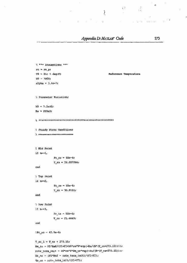
Appendix D: MATLABG Code 173
'Zi * ** Assurnption.s Ie **ro ro_p:TO 25: " deg(C)HO 3000;
Heference Temperature
alpha ~ 3.4e-7:
Paremeter V<1riat.ion;
1:0 7.1e32:Ea 203e3;
11 **************************************************
" St:eady state Conditions
'0 Mid Pointif n=~l,
FC_55 ~ 50e-6:T_E5 ~ 26.057964:
end
',', Top Point
if n~=2t
FC_55 ~ 50e-6:T_ss ~ 30.9101;
end
':,LOI'1Point
Fc_"s ~ 50e-6;'j' DS 'c 21./l649;
end
',';Pc s s 42.ge-6;
}[1\l~S[J Fl ">:mfl (F1+F2-1 J:O*ro*V*e::p(-Ea/ {R* ('r_s,'J+273 .15))));rate,,~t.Q):m ..iIlit ~ J:O*ro1.V*Xm,_J3s*el:p (-Ba/ (R* (T~"'s+,273 .15»);
(E'l*Xnf _, r:ate,tenu_init)!{Fl+F2);
r:dtl'_ tnrm __inj,tl (F1+1:'2);

i\_),
Appendix D: MA7LtiBO Code 174
':i Derived Steady State Conditions
Beta_ss :oo_"ss*Cpm + Xn_ss*Cpn + Xp_ss*Cpp + '"
(I _ Xm_ss - Xfl_SS - Xp_ss)*Cpi;
u ~ 1/«I/UO) + alpha * Fc_ss"(-0.8»;
Teo (U*Ac*'I'_SS + 'I'ei'" (Fc_ss*4186e3 _. U*Ac/2» I. "
(Fc_ss*4186e3 + U*Ac/2);
Tave_ss ,~ (Tei + 'rca) /2;
q_.ss U*Ac*(T_Ss - Tave~os}i
Gamma ss Joo_ss* (dHtm + Cpm* ('1'_S5-TO» + .•.
Xn_f.!'!* (dRtn + Cpn* (T_5S-TO» +
XP_5S* (dHtp + Cpp* ('1'_5S-TO» +
(1. - Xm_5S _ Xn._ss -XI'_55) * (aHti + Cpi< ('1'_ss-TO) ) ;
alpha_ss 0;
(l?1* (Xmf* (dHfm + Cpm*(TI-TO» + (1 Y.mf) * (dHii -1- Cpi" (TI-TO) ) ) + •••
F2*(XnZ*(dHfn + Cpn*(T2-TO» + (1 - }\nf)* (dHfi -1- Cpi*('1'2-TO»»;
TB_ss (C - q_ss - (Fl+F2) *Ga.'11ll\a_ss - V"ro;'alpha._ss);
k_ss j:O*V*ro*exp (-Eal (R*T_ss_kl ) ;
.,**************************************************
Pattial DifferentiuJ ..';
dU_d~'c O. 8*alpha* « (l/UO) !-alpha*Fc_ss" (-0.8) )" (-·2» *Fe_ss" (-1. B) ;
';, output '1'emperature ('l'co)
d'I·co._dT
dTco_dFC
tPAcl (FC_.55*1000*4186+ {U*Ac/2»;
(dU_dl"c*lIc*T_ss + Tci*(4186€,j - dU_dFc*Ac/2»* ••.(Fc_ss*41B6e3 + U*Ac/2) h (··ll +
(U*Ac*T_ss + 'rci* (Fc_.ss*l1186.3 - U*Ac/2» * •••

Appendix D: MATLAB~ Code
(-1) * [4186e3 + dU_dFc*Ac/21 * (Fc_sr;*4186e3 + U'kAc/2) A (-2);
", Average Temperatm:e
dTav_dT ~ 0.5*dTco_dT;
dTav_dFc = O.5*dTcO_dFC;
"; q - Ellergy from system
dq_dXm 0;dq_dXn 0;
dq_dXp 0;dq_dT U*Ac - U*Ac*dTav_dT;
dq_dFc dU_dFe * AC*T_ss - dU_dFc*Tave ss*Ac - d'fav_dFc*U*Ac;
n, dalpha - differantial term;
dalpha~dXm = G;dalpha_dXn = 0;dalpha_dXp = 0;dalpha_dT 0;
dalpha_dFc 0;
n, Beta
dBeta._ dXnt = Cpm - Cpi;
dBeti1 dXn Cpn - Cpi;
dBeta_dilp Cpp - epi;
dBeta dT 0;dBeta _dFe 0;
" Gamma -
dGalTlIll2t__dxm ~~ [dHfm + cpm * ('I'_Ss - 1'0» - dHfi - Cpi* (T_ss - TO);
dGamma_dXn (dRfn + Cpn * (T_ss - 10» - dHfi - Cpi*(T_ss - TO);
clGam.na__dl(p (dHfp + Cpp * (T_S3 - '.r0» _ dRE - Cpi* IT_ss - TO):
dGalTlIlla__dT Xm_ss*Cpm + Xn__ss*Cpn + XP_Ss*Cpp +
(1 - Xm_ss - Xn_ss - Xp_ss)*Cpi;
dGarruna_dFc 0;
\'; Temperature
dBeta2_dXm ~ (-,1/ (Beta_ss"2) ) *dBeta_dXm;
175

ciBeta2_dXndBeta2_dXpdBeta2_dTdBeta2_dFc
Appendix D:MATL1B~Code 176
(-1/(Beta_ss"2» *clBeta_dXn;(-1!(Beta_ssA2»*dBeta_dXpi(-11 (Beta_ss"2» *dBeta_dT;(-1/(Beta_ssA2»)*dBeta_d2c;
dTB dxn
dTB_dY..m ~ (-dq_rL\I;u, •. (Fl-t-F2) *dGamma_diLT - V*ro*dalpha_dXm);
dTB_~lXp
dTB d'!'
dTB dFc
(-dq_cll(n _ (Fl+F2) *dGamma_dXn - V*ro*dalphae,cL'{n);
(-dq_dXp - (Fl'!-F2) *clGaroma_dXp - V*r0*dalpha_dXp);
r-dq_oI - (Fl+F2)*dGarmna_dT - V*ro*dalpha_dT);
(-dq_dFc - (Fl+F2) *dGam;l1a_dFc - V*r:n*dalpha._dFc);
d'r_dJ(ffi ~ (11 (V*r0» * (dBeta2_dXm * TB_ss + (l/Beta_ss) *dTB_dX!l1);
dT_dxn (11 (V*ro)" (dBeta2_d]{n * TB_Ss + (l/Beta_ss) *dTB_dXnl;
dT_d:;p (11 (V*ro»" (dBeta2_dXp * TB_ss + (I/Beta_ss) *dTB_ciXp);
dT_dT (11 (V*ro) l" (dBeta2_d'1.' .. TB_ss + (l/Beta._ss) "dTB_dT.);
dT_dFC (1/(V*ro»*(dBeta2_dii'c .. TB_ss + (1/Ileta_5s)*riTB_dFc);
" Xm concentration
dk_dxn-. = 0;
dk_dXI1
dl:_dXp
dk_dT
dk_dFc
0;0;kiI~'ro*V* (Ea/R) * (11 (T_ss_k"2J ) *e};p (-Eal (R*T_5S_kl) ;
0;
dJ:m_clXn
dXm_dXm ~ (1/(v*ro»*(-FI-F2-k_ss);
dXm_dXp
dXm_d1'
dXm._dE'c
0;0;- (11 (V*!;o» *)(m._ss*dk_dT;
0;
" l{n Concentration
dXu_dXm '" -k_5S/ (l:O*V) ;
rlXn__dXn (1/ (ro*V»" (-Fl-F2);
dXn_d:(p
dXll_d'J'
dXll_dFC
0;- (11 (V*ro» "Xm_ss*dk_dT;
0;
" Xp concent rat.Jon

AppendixD:MATLAB" Code
d:;p_dXm = k_ss/ (ro"'!);
dXp_dXn
dXp_dXp
dXp_d'l'
dXp_dFc
0;(1/(V*rol)*(-FI-F2);
{II (V*ro)) 1:i{n_ss*dk~d11;
0;
~ *******************************************
n State ::'.~ace
A [dYm_dXmclXIJl__dXn dXm_dXp dXm_dT; .•.
dXn_dXm dXn_dXn dXn_d.Xp dXn_dT; ••.
dXp_dY.mc:xp_cLXndXp_dXp dXp_dT; •.•
dT_w.m dT_dXn dT_dXp d'r_dT];
B [dXIJl_dFc;dXn_dFc;dXp_dFc;dT_dFc];
C [0 () 0 1];
'"C [1 0 0 0];
D [OJ;
[nurn,denj ~ ss2tf(A G,D);[z,p,k] = tf2zp(num,den);
disp\'Results :');
disp(['Gain :']);
disp(k);
disp(['Zaros :']);
disp(z};disp(['Poles :']);
disp (p);
da sp t ' •••••••••••••••• ');
disp ( 'Transfer Function');
da sp tnum) ;
disp ( ,-.------ ---------------------------, ) ;
diap Idon) ;
':;Removepoles/;:eros that cancel
d~sp(' ');
[num_mill, den jni n] =mi.nz ea l (num, den) ;
dis.',) ( , 11inm!.sc"d Transfl2r Function is :');
177

Appendix D: Mi1TLAB$ Code-~----~-.~-----~---~---------------------
disp (numrni.nj r
disp ( ,------------------------.------------------, ) ;
disp (den_min) i
d.isp t ' ');
IZt"P/J~J tf2zp (m:m_min, den_min);
disp(['Gain :']};
disp(k};
disp ( [ 'Zeros :']);
disp(z);
disp(['Poles :']);
disp(p) ;
D.2.3 i cstr.m
k**********************************~****
<j -k** Initialise SJ.mulink CSTP.Model +**~ *~**************************************
~ By S~D.FlorenceFirst Edit: October 1995
n. Last Edit : June 1996
Initialise the CSTR simulation
n. For use ~1ith Simulink modeI
o, Inputs : None
, Outputs : Variables to workspaco
<::1c:;
c1isp (- Clearing Variables .•.• ' );
di.sp('Initialising Vadables ••• ·);
c'.Hfm ~ -640e1; " ,;.mole(-l)
Cpm ~" 32.0(1; ';, ,J.mole(-ll.der Iq-l~
ro_m '" 55506; c" mole.m(-3)
Heat of Formation of M
Specific heat of H
Density of N
TI 18; 'cO; deg(C:, T(;mperature in
PI 3.60789;
)(mf '" 0.002;
Ii,
178

,j
----.--_"-~----Appendix D: Mil T'...AB- Code 179
dHfn = ,,740e3: J.mole(-l)Cpn '" 2.9.00; ':i J.mole(~l) .deg 1((-1)
LO_l1 ~ 55506- '~\rnole.tr.(-])
T2 18; deq(C)P" .3.60789;
xru ,~ 0.08;
*** Inerts ***dHfi ~ -571. 68e3: '" J.male(-l)
Cpi ~ "i5.415: " J.mole(-l) .deg K(-1)
ro_i ~ S5501i; " rrale.m(-'3)
~ .** P flow·'·ro_p~.'Hfp
55506; ';; mal,~.m(-3)
-2,100e3: ~i J .mo Le (-1)Cpp'" 61.00: '" J.mole{-l) .C{-l).ro__P ~ 55506; 'J mol,".m{-3)
~ *** Constants ***kO 7.1e32; ':' s{-l.)
203e3; ';; ,I.male(-l)Ea
h 0.28: \,ms=O.41:n·m
V (s=s) *h: ?: m~3)
" **. Cooling Coil ***
'rei ~ 18; '0
coil_di,ameter '" (1. (l15;
coil~diam(,ter_Ln = O.Ol38;
Goil_length'" 6."008;V_coil '" coil_length*pi* (coil_diameter_inn) ~2;
Ac "' cOl~_length"2*pi *coil_diameter/2;
,,';*** Assumptiuns 'A**
1:0 ro._p;
TO 25: ':i deg (C)UI) 3000;
,,1ph2 ". 3.4e-7;
Heat af Formation of NSpecific Heat of NDensity of NTemperature in
Heat of formation of inertsgpecififc Heat of in2rtsDensity of ine~ts
Density of l?
Heat. of formation of l?
Specific ~eat of PDensity of P
Pre-expo kinetic rate constantR ~ 8.3144; '" J.mole.C(-l)Ic'cal gas constant
Initial HeightSideVolume
!nirial Temperature of inert
Reference Ternpel'ature
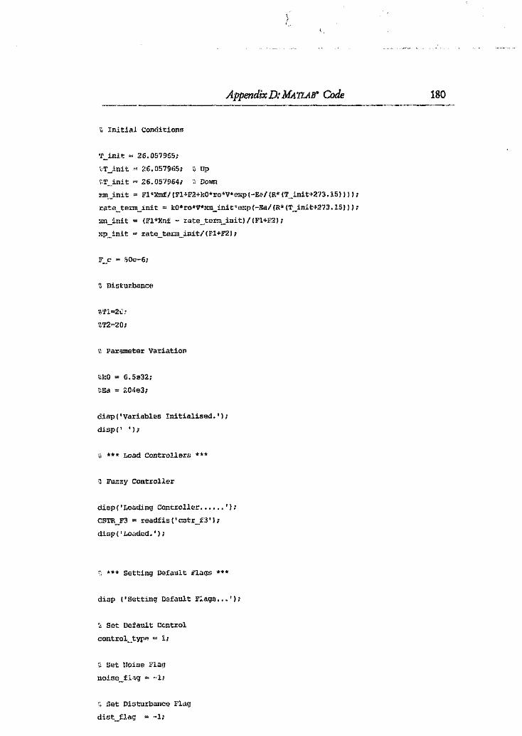
Appendix D: MA'!LAB· Code-_-----_.----
" Initial Conditions
'P_inlt ~ 26.057%5:
'"T_init
""T_init
26.057965; u Up
26.057964; "Do:-m
xm__init F1"Xmf/ (FHF2+l~O*ro*V*el:p (-E0/ (R*(T_init+273 .15) ) ) );
rate_terID_init = kO*ro*V*xnl_init-'e;-:p (-Eal (R*('I'_init+273 .15) »;::n__init (Fl*Xnf _. rate_term_init) I (];'1+E'2);
l:p_init rate_term_initl (Fl+F2);
F_c 50e-6;
':, Distur.bance
?;T2==20;
':i Par ametier; Variation
C,';}:O 6.5332;
';;Ea 204e3;
disp('Variables Initialised.');
disp t ' ');
':, *** Load Controllers ***
" Fuzzy Controller
disp('Loading Controller ..••.. ');
CSTR_F3 = readfis ('cstr_f3');di sp ( ,Loaded. ' ) ;
_,*** setting Default ""lags ***
disp ('Setting Default F::'ags ..• ');
',\ Set Default Control
control_typA = 1;
,;, Set !loise Fla9
noc.sc ....,fl.1g :.;.;·~l;
'.', Set Disturbance Flag
dist __flag = -1;
180

Appendix D: M41ZAB& Code 181
disp ( 'FJ.acys Set.'):
disp{ ,
dlap ('CS'l'P. Initialised.');
D.2.4 qft_cstr.m
*************k**~***~******
*** QFT Design for CSTR ***" ***************************
',; Author: S. Florence
n. First Edit : February 1996
~ Last Edit : June 1996
n Interactive design for CSTRo Requi!""s the QFT tooLbox
.' Inputs : None
"-i Outputs : Graphics, and variables as selected
" Specs as lJiv,"n in main report
clear;
pst'? 1· p., 0 Pause flag
clc
echo off
clc
PROBLEDl DATA
','; compute the boundary of the plant templates
disp ( IComputing plant templates.... ')
dralIDOI"I
r = 1; k = 8.8431e1; b = 4.815ge-l; ct = 8.5546e-3;for e = -[1.3253e-6 1.ge-6 2.5e-6 3.2114e-6],nump(c,:) ee [J{,b]; denp(c,:) ~ [I,d,e]; c ~ c + 1;
end
t = 8.8431e1; b = 4.81598-1; d = 9.5561e-3;for 8 = -[1.32538-6 1.98-6 2.58-6 3.21148-6],

Appendix D: MATLAB" Code
[k,b]; denp(c,:)nurop{c,:)endk ~ 8.8431e1; b = 5.6840e-1; d = 9.556]e-3;
c + 1;
for e = -[1.3253e-6 1.ge-6 2.5e-6 3.2114e-6],nurnp(c,:) = [k,b]; denp(e,:) = [l,d,e]; c ~ C -1- 1;
endt = 8.8431el; b = 5.6840e-l; d = 8.5546e-3;for e = -[1.3253e-6 1.98-6 2.5e-6 3.2114e-61,l1ump;c,:) = [k,bJ; denp,c,:j = [1,dteJ; e = c + 1;
end
k = 1.1080e2; b = 4.815ge-1; d = 8.55468-3;for e = -[1.3253e-6 1.ge-6 2.5e-6 3.2114e-6J,nump j c. r) = [k,b]; denp(c,:) = [l,d,e]; c = c + 1;
endk = 1.1080e2; b = 4.81598-1; d = 9.5561e-~;for e = -[1.3253e-6 1.ge-6 2.5e-6 3.2114e-6],nump(e,:) = [k,b]; denp(c,:) = [l,d,eJ; c = ~ + 1;
endk = 1.1080e2; b = 5.6840e-l; d = 9.55618-3;for e = -[1.3253e-6 1.ge-6 2.5e-6 3.2114e-6],nump(c,:) = [k,bJ; denp(c," [l,d,e1; c = c + 1;
endk = 1.1090e2; b = 5.6840e-l; d = 8.5546e-3;for e '"-[1.3253e-6 1.ge-6 2.58-6 3.2114e-6J,!lump(e,:) = [k,b]: denp(c,:) = [l,d,e]; c e- c + 1;
end
'xU Nominal Plant ***
nump(e,:) ~[9.9281e+001r 5.3098e-001J;denp(c,:) ~[1.0000e+000, 8.9364e-003, -2.58008-006]; c~ c+l;
diSp('No of Plants :');
disp(c-l);
disp(' ');
nompt c-l; ':i define nominal plant case
" Compute ;:-f~[;pOn,ses
t1 ~ [0.0001,.001,.0).,.1,1];)?~"fr(?qcp(nump,denp, :~);
182

Appendix D: .MA TLAB· Code 1.82
I1.WVP(,:,: }
.nd
k = 8.8431e1; b = 5.6840e-1; d = 9.5561e-3;
[1:,b]; d,::',p{c,:) [l,d,e): c = c + 1;
for e = -[1.3253e-6 1.ge-6 2.5e-6 3.2114e-6],nump(c,:) ~ [k,b]; denp(c,:) '" [l,d,e]; c '"c + 1;
end
k = 8.8431e1; b = 5.6840e-1; d = 8.5546e-3;for 0 ~ -(1.3253e-6 1.ge-6 ~.5e-6 3.2114e-6J,nnmp(c,:) = [J:,bJ; denp tcv r) = [l,d,el; c = ,•• 1;
end
1: = 1.1080e2; b = 4.815ge-1; d = 8.5546e-3;e = -[1.3253e-6 1.98-6 2.5e-6 3.21146-6J,
nump(c,:) = [k,bJ; denp(c,:) = [l,d,el; c = c + 1;endk = 1.108082; b = 4.815ge-1; d = 9.5561e-3;for e = -[1.3253e-6 1.ge-6 2.5e-6 3.2114e-6],GWup(c,:) = [k,DJ; denp(c,:) = (l,d,eJ; c = c + 1;
endk = 1.1080e2; b = 5.6B40e-1: d = 9.5561e-3;for e = -[1.32538-6 1.ge-6 2.5e-6 3.2114e-6I,nump(c,:) ", [k,D]; rl;',np(c,:)'" [l,d/eJ; c = c + 1;
endk = 1.108082; b = S.6840e-1; d = 8.55~6e-3;for. e = -[1.3253e-6 1.ge-6 2.5e-6 3.2114e-6J,nump j cj r ) = [k,b]; denp Icy r ) '" [l,d,e]; c = c + 1;
end
"i **', Nominal Plant ***
nump(c,:) ~[9.9281e+001, 5.3098e-001];
denp(c,:) "'[1.0000e+000, 8. 936,le-003, -2.5800e-006]; c= c+l;
disp ( INo of Plants : I ) ;
disp(c-l);
disp( I ');
nompt c-l; ". def Lne nominal plant case
'" ccmput e responses
1·/ '" [0. COOl, .001,•:)1, .I,lJ;P~"freq:::p(nump,denp, \'1) ;

Appendix D: MATLAB~ Code
disp ( INo of freq points
dl sp (le::lgth ('~I " ;
disp(' ');
.1\ •. /'
dispi' ')
disp (' plottmpl (1'1, ~l, P, nompt); '/'ShO\'1 templates I )
dr awnow
plottmpl (v1, \'], P, nompt), title (' Plant Templates ')
if pse qpause; end
close(gcf);
'i; *** Robust 11argin ***
d l sp I" I)
disp(IComputing bounds .•. 'l
disp(I ')
disp (' bdb l=sf.soonds (1, \'1,wbdl , til, P, R,nompt); '!;margins ")
dravmO\v
I"bdl ~ [.0001,.001,.01,.1,1J; 'I; compute bounds at all frequencies in Iv
I'll ~~1.2; ?i de tine .,eight
bdbl ~ sisobnds(2,w,wbdl,111,P,R,noropt);
disp (' plotbnds (bOO1); ',;shoN bounds ')
plotbnds (bdbl) r ti tLe ( IRobust ~largins Bounds I ) ;
~f pse qpause; end
close(gcfl;
*'h Output Disturbance ***
disp(I ')
d LSP('bdb2~sisobnds (2, u, \1bd2, \'12,P, R,nompt l ; ';,output disturbance rejection ')
dz awnow
\~bd2~[.OOOl,.(J01,.OlJ; "the frequency array
r'j2~abs (freqcp ([1,1. 01e-l, 1e-4], [1,2.01,1. 02, 1e-2J I N)I;
bdb2 ~ s isobnds (2, \'1, \']bd2,\']2, P, R,nompt) ;
disp ( 'plotbnds (bdb2); ',isho,,] bounds' )
dz awnow
plotbnds (bdb2l, title('Hobllst Output Disturbance Rejection Bounds');
183

Appendix D: MATLAB0 Code------
184
if pse qpause; end
clos'= (get) ;
;.** Input Disturbance Bounds ***
ddsp t ' ')dz sp {' bdb3~.sisobmls (3, tv,Hbd3, 1']3,P, R,nompt); ',;input disturbance reJection' j
dr awnow
;;bd3~ [ •0001, •001, .01]; '; the frequency array
\'/3 ~ 1000; ~i define Iveight
:';I'13=o3bs(treqcp (100* [1, 1.Ole-I, 1e-4J, [1. J. 01, 1.02, 1e-2J, w) ;
bd',,3 ee sisobnds (3,1'/,vibd3,\'13, P, a, nO!l1pt);disp ('plotbnds (bOO3); 7;shOl']bounds')
plotbnds(bdb3),title('RoDust Input Di.sturbance Rejection Bounds');
if pse qpause; end
close (gef) ;
disp(' t)
disp ( 'bdb=grpbnds (bdbl, bdb2); 'i,grouping bound,;')
dialmO\']
bdb=qrpbnds (habl,bdb2);
d:isp,'plotbnds(bdb); ,;\shml all bounds')
plotbnds lbdb) , title (' A"-l Bounds');
U: pse qpause; end
cl.ose (gcfl;
a1.Sf (' ')
uf.sp (' ubdb=sect.bnds (bdb); '(,intersect bounds')
dl~aI-mO\';
ubdb=sectbnds(bdb);
di.sp (' plotbnds (ubob); ShOH hounds' J
dr atcnow
plothnds (ubdb) , title t ' Intersection of Bounds');
if pse qpauser end
close(gcf);
_, *~~~******-.l '1:11'********** DESIGN ***~"****************'!<r****1t**
dj.sp(' ')
disp ( 'Design' )
dd sp (' Lpshape (~Il, UbrJ.b,nLO, dLO, delO, ncO, ,kO); ':.loop shaping')
disp(' ')
nGO~[1 ;dcO=[j; Initial controller

Appendix D: MA 71..A.3S Code 185
'2; cont ro l l.er 1 - causes oscil1ations
~kO = (.2479*0.00876*3.11/.1961)*(i.789*4.789);
~[ncOfdcOJ~zp2tf,[-.1961J, [-O.008876,-3.11,-0.B43B+4.714i,-0.8438-4.714i]',kO);
" Controller 2 - Alsc Oscillations
~;J;O "" (.::A47"0.00876*8.397*6*6/.196l);
~[nc0,dcO]~zp2tf([- 1961], [-0.008876,-8.397,-4.8+3.6i,-4.8-3.61] ',kO);
~kO = (.005171*0.0009226*0.4868/.0138);
'HneO, dcO]=zp2tf (l-'O. 013S], [-0.0009226, -0.4868] , , kO);
~ Fin.l controller
kO = (0.001806*1.321*3.631);[ncO, deO] =zp2tf ([], [-1. 321, -1. 631] , r kO);
wI = .logspace(-5,2,lCO); 'i; define a frequency array for loop shaping
nLO=nump(nompt,:); dLO=denp(nompt, :);
delOc,O; ',', no delay
lpshape (;11, ubdb, nLO,dLO,delO, nco, dcO);
qpause;
numC=ncO; denG"'dcO;
"l ANALYSIS
disp{' .)
disp ( 'l'.nalysi.s •••. ' )
disp ( 'He-define a more dense plant template (100 points) ...• ' )
dralmow
P~freqcp(nt1mp,denp,lvl) ;
G'=freqcp (numc, denC, I'll) ;
dispe' , J
disp (' cnxai so (1, I'll, ~11,P, H,G); ~;margins spec')
drawnow
chkai so (I, I'll, I'll, P, H, G) ;
qpause;close(gcf);
di.sp t ' ')
disp (' chksa so r2, \'11,'1'12, P, R, G); ':,output disturbance rejection spec')

Appendix D: MATLAB~ Code
draHl10N
ind~find(wl<=lOJ;
\'12~abs (freqcp (0. 02* [I, 64,748,2,100], [1,14.4,169], .vl»;
chks i so (2, \11(ind) ,N2 (ind),!? (:, ind), tt, G(::'nd) ) ;
qpause;close(gcf);
d.i.ep t ' .)
disp (I chks i.so ~3,HI, v13, P, R,G); ~:;input dj sturbance rejection spec')
dr ;-11101'/
chksiso (3,v/1(ind) , 1'13, P (:,ind) r Ro'G (ind») ;
qpause;close(gcf);
186
References 187
References
1 Radecki T. An evaluation of the fezzy set theory approach to information
retrieval, in Trappl R., Findler N.V. and Horn '1/., Progress in Cybernetics and
Systems Research, Vol. 11 : Proceedings of a Symposium organised by the
Austrian Society for Cybernetic Studies, Hemisphere Publishing Company,
1982.
2 Zadeh, L.A. A fuzzy-algorithmic approach to the definition of complex or
imprecise concepts, Systems Theory in the Social Sciences! 1976, pp 20i.
3 Zadeh, LA Fuzzy Sets, Information and Control, Vol. 8, 1965, pp 338-353.
4 Zadeh, L.A. Outline of a new approach to the analysis of complex systems and
decision processes, IEEE Transactions on Systems, Man and Cybernetics, Vol.
SMC-3, No.1, 1973, pp 28-44.
5 Zadeh, L.A. Calculus of fuzzy restrictions. In L.A. Zadeh, K.S.Fu, K. Tanaka
and M. Shimura (editors), Fuzzy Sets and Their Applications to Cognitive and
Decision Processes,Academic Press, 1975, pp 1-39.
6 Mamdani, E.H. Application of fuzzy algorithms for control of a simple dynamic
plant, Proceedings of the IEE, Vol. 112, 1974,pp 743-753.
7 Mamdani, E.H. and Assilian, S. A fuzzy logic controller for a dynamic plant,
International journal ofMan-MachineSttidies, Vol. 7,1975, pp 1-13.
B Kickert W.].M. and van Naute Lemke H.R. Application of a fuzzy controller in
a warm water plant, Automatica, Vol. 12, 1976,pp 301-308.
9 Pedrycz W. Fuzzy Control and Fuzzy Systems, 2nd (extended) edition, Research
Studies Press Ltd. England 1993.
10 Jager, R. Fuzzy Logic in Control, PhD Thesis, Technical University Delft, 1995.

\,
References 188
11 Mendel, J.M. Fuzzy Logic Systems for Engineering: A Tutorial, Proceedings of
the IEEE, VoL 83, No.3, March 1995, pp 345-377.
12 Kosko, B. Neural Networks and Fuzzy Systems: A Dynamical Systems Approach to
Machine Intelligence, Prentice Hall Inc, 1992.
13 Sugeno, M. Industrial Applications of Fuzzy Con vol, Elsevier Science Pub. Co.,
1985.
14 Heckenthaler T. and Engell S. Approximately time-optimal fuzzy control of a
two-tank system, IEEE Control Systems, June 1994, pp 24-30.
15 Jang, J.S.R. and Gulley, N. Fuzzy Logic Toolbox for Use with llMTLAB, The
Mathworks Inc., Natick, Mass, 1995.
16 Shaw, I. Introducing Fuzzy Logic, Compuiecb, Vol. 8, No.3, March-June 1992.
17 Apptronix Inc, Fuzzy Logic - From Concept to Implementation, Doc. No.
EDU01V10-0193, 1993.
18 von Altrock C. NeuroFuzzy Technologies, Sensor Review) Vol. 12, No.3.,
1994, pp 15-17.
19 Bannatyne R. Development of fuzzy logic in embedded control, Sensor Review,
Vol. 14, No.3, 1994, pp 11-14.
20 Kong S.G. and Kosko, B. Adaptive fuzzy systems for backing up a truck-and-
trailer, IEEE Transactions on Neural Netwotks, Vol. 3, No.2, March 1992, pp
211-223.
21 Li, Y.F. and Lau C.C. Development of fuzzy algorithms for servo systems,
IEEE Control Systems Magazine, Apri11989, pp 65-71.
22 Pritchard, C.j. Determining signal levels in robustly controlled plants using
frequency domain closed loop system specifications, PhD Thesis, University of
the Witwatersrand, 1995.

References 189
13 Thomas, D.E. and Arrnstrong-Helouvry B. Fuzzy logic control- A taxonomy
of demonstrated benefits, Proceedings of the IEEE, Vol. 83, No.3, March 1995,
pp 407-421.
2·} Pfeiffer B. and Isermann R. Criteria for successful applications of fuzzy control,
Engineering Applications of Artificial Intelligence, Vol. 7, No. .3, 1994, pp 245-
253.
25 Kosko, B. Fuzzy Tbinking: T7JeNew Scienceof Fuzzy Logic, Flamingo, 1994.
26 Black, M.Vagueness: An Exercise in Logical Analysis, Philosophy of Science,
Vol. 4, 1937, pp 427-55.
27 Zadeh, L.A. The concept of a linguistic variable and its application to
approximate reasoning, Information Sciences, Vol. 8, pp 199-249, and Vol. 9,
1975, pp 43-80.
28 Sugeno, M. Fuzzy measures and fuzzy integrals : a survey, In M.M. Gupta,
G.N. Sardis and B.R. Gaines (editors), Ft}zzy Automata and Decision Processes,
North-Holland Publishers, 1977, pp 89-102.
29 'Yang, L.X. arid Mendel, J.M. Fuzzy basis functions, universal approximation
and orthogonal least square learning, IEEE Transactions on Neural Networks,
Vol. 3, 1992, pp 807-813.
30 Kosko, B. Fuzzy systems as universal approximators, IEEE International
Conference on Fuzzy Systems, 1952, pp 1153-1162.
31 Procyk, T.J. and Mamdani, E,H. A linguistic self-organising process controller,
Automatica 15, 1979, pp 15-30.
31 Bartos, F.J. Fuzzy logic continues to grow, well guarded by user's wraps,
Control Engineering, September, 1994, pp 47~51.
.13 Shahian, B. and Hassul, M. Control System Design using .MA TLAB, Englewood
Cliffs Prentice-Hall, 1993.
References 190
34 Horowitz, I.M. Qttantitath'e Feedback Theory (QFI), Volume 1, QFT
Publications, Boulder, Colarado 80303, 1992.
35 Azvine, K and Wynne, R.J. A review of quantitative feedback theory as a
robust control system design technique, Transactions of The Institute of
Measurement and Control, Vol. 14,No.5, 1992,pp 265-279.
36 Borghesani, C Chait, Y and Yaniv O. Quantitative Feedback Theory Toolbox for
use with MATLAB', The Math'\}7orksInc, 1994
37 Driankov, D. Hellendoorn, H. and Reinfrrrk, M. An Introduction to fuzzy
control, New York, USA, Springer-Verlag, 1993.
38 Malki, H.A., Li, H. and Chen, G. New design and stability analysis of fuzzy
proportional-derivative control systems, IEEE Transactions on Fuzzy Systems,
Vol. 2, No.4, pp 245-254.
39 Johansen, T. A. Fuzzy Model Based Control: Stability, Robustness ..rId
Performance Issues, IEEE Transactions on Fuzzy Systems, Vol. 2, No.3, 1994, pp
221-233.
40 Tanaka, K. and Sano, M. A robust stabilisation problem of fuzzy control
systems and its application to backing up control of a truck-trailer, IEEE
Transactions on Fuzzy Systems, Vol. 2, No.2. 1994,pp 119-133.
41 Tanaka, K. ana Sugeno, M. Stability analysis and design of fuzzy control
systems, Fuzzy Sets and Systems 45, 1992,pp 135-156.
42 Chen, C., Chen P, and Chen, C. Analysis and design of fuzzy control system,
Fuzzy Sets and Systems 57, 1993, pp 125-140.
43 Mamdani, E..H. Twenty years of f,lZZY control : experiences gained and lessons
learnt, IEEE, 1993,pp 339-344.
44 Deshpande, P.B. and Ash, R.H Elements of Computer Process Control with
Aduanced Control Applications, Instrument Society of America, 1931.

References 191
45 Macl.eod, I.M A controller incorporating a fuzz}' logic adaptive mechanism for
processes with long dead times, Fuzzy Logic in Control Systems, Rand
Afrikaans University, Auckland Park, October 19~2, South African Council
for Automation and Computation.
46 Rodd, M.G., Verbruggen H.B. and Krijgsman A.j. Artificial intelligence in real-
time control, Engineering Applications of Artificial Intelligence, Vol. 5, No. :),
1992,pp 385-399.
47 Rodd, M.G. Safe AI - is this possibles, Engineering Applications of Artificial
Intelligence, Vol. 8, No.3, 1995,pp 243-250.
48 Umbers I.G. and King P.]. An analysis of human decision-making in cement
kiln control and the implications for automation, International [oumal of Man-
Machine Studies, Vol. 12, 1980, pp 11-23.
49 Bernard, J.A. Use of a rule based system for process control, International
Conference on Industrial Electronics, IEEE Control Systems Magazine, October
1988, pp 3-12.
50 Song, J.J and Park, S. A fuzzy dynamic learning controller for chemical pn ess
control, Fuzzy Sets and Systems 54, 1993,pp 121-133.
51 Feng, F.C. and Sheng, N.Y. Application of fuzz: logic in the speed control of
ac servo systems and an intelligent inverter, IEEE Transactions on Energy
Conversion, Vol. 8, No.2, June 1993,pp 312-318.
52 Assayama, H., Burton, P., Gerstacker, }., Kohono, T. Matsui, S. and
O'Lionaird, E. Fuzzy logic control of perlite plant, Computing and Control
Engineering journal, IEEE, December 1994,pp 293-298.
53 D' Azzo, J.} and Constantine, H.H. Linear Control System Analysis and Design :
Conoentionnl and Modern, McGraw-Hill, 2nd Edition, 1~81.
54 Gordon, A. The Design and Construction of a Prototype Testbed for Laboratory
Experimentation and Controller Testing, MSc Project Report, University of the
Witwatersrand, 1996.

\\,
References 192
55 Balchen, J.G. and Mumme', K.I. Process Control: Structures and Applications,
Van Nostrand Reinhold Company, New York, \988.
56 Stephanopoulos, G. Chemical Process Control : An Introduction to Theory and
Practice, Prentice Hall, New Jersey, 1984.
57 Horowitz 1. Quantitative feedback theory, lEE Proceedings Pt. D : Cont-rol
Theory and Applications, VoL 129, No.6, 1982, pp 215-226.
58 Roffel B. and Chin P. Computer Control in the Process Industries, Lewis
Puixishers, USA, 1937.
59 Deshpande, P.B. and Ash, R.H. Elements of Computer Process Control with
Advanced Control Applications, Instrument Society of America, 19l:l1.
60 Lovrich, A.I. and Hellenthal, B. Servo Control of a DC-brush Motor using
Fuzzy Logic, Quantum, 1995,pp 21-23.
61 Efststhiou J. Expert systems, fuzzy logic and rule-based control explained at
last, Trans. Inst. M.e, Vol. 10, No. 4, July-September 1888,pp 198-206.
62 Redelinghuys D. and Stothert A. The myth-application of fuzzy logic,
QttantHm, June 1995,pp 16~20.


Author: Florence, Stuart Douglas.Name of thesis: An investigation into the merits of fuzzy logic control versus classical control.
PUBLISHER:University of the Witwatersrand, Johannesburg©2015
LEGALNOTICES:
Copyright Notice: All materials on the Un ive rs ity of th e Witwa te rs ra nd, J0 han nesb u rg Li b ra ry websiteare protected by South African copyright law and may not be distributed, transmitted, displayed or otherwise publishedin any format, without the prior written permission of the copyright owner.
Disclaimer and Terms of Use: Provided that you maintain all copyright and other notices contained therein, youmay download material (one machine readable copy and one print copy per page)for your personal and/oreducational non-commercial use only.
The University of the Witwatersrand, Johannesburg, is not responsible for any errors or omissions and excludes anyand all liability for any errors in or omissions from the information on the Library website.
Top Related