


Languages
Pages
Legal


Analysis of Limited Area Models for Wind Power Prediction
Enel Green Power, Innovation and Sustainability:
Federico Fioretti, Fabrizio Bizzarri, Gianmatteo Cirillo
Enel Green Power, Europe Area, Commercial Officer: Claudio Pregagnoli
Enel Ingegneria e Ricerca, Research and Innovation: Umberto De Angelis
CNMCA National Meteorological Center of the Italian Air Force:
Francesca Marcucci, Lucio Torrisi, Roberto Tajani
Abstract: Allo scopo di migliorare l’accuratezza delle previsioni per impianti rinnovabili di generazione elettrica alimentati da fonte eolica, un nuovo modello NWP (Predizione Numerica del Tempo) è stato testato come input ai modelli statistici sviluppati dall’ENEL. I campi di previsione forniti dal modello operativo NWP (COSMO-ME) del Servizio Meteorologico dell’Aeronautica Militare sono stati usati e confrontati con un sistema di riferimento interno
dell’ENEL, basato su un differente modello NWP, per valutare le prestazioni per le previsioni di energia eolica per il giorno stesso e per il successivo. I test sono stati effettuati su un numero significativo di parchi eolici per verificare l’affidabilità del lavoro. La prestazione di COSMO-ME è molto buona rispetto alla predizione per il giorno stesso, ma sembra sostanzialmente allineata rispetto al modello per quanto riguarda le previsioni per il giorno successivo.
Abstract.
In order to improve the accuracy of wind power predictions, a new mesoscale NWP (Numerical Weather Prediction) model was tested as input to the statistical downscaling models developed by ENEL. Forecast fields provided by the operational CNMCA NWP model (COSMO-ME) were used and benchmarked to a reference ENEL’s internal system, based on a different NWP model, to evaluate performance on intraday and next-day wind power predictions. The test has been carried out on a significant number of wind farms in order to assure work reliability. COSMO-ME performance is very good with regard to intraday predictions but seems substantially aligned with the reference model for what concerns the next day predictions.
• Keywords: wind speed forecasting; wind power prediction, neural network, limited area models,
energy yield forecasting.
1 Foreword
Enel Green Power (hereinafter ENEL GP) is the Enel Group Company
dedicated to developing and managing energy generation from renewable
sources at an international level, with a presence in 17 Countries among
Europe, the American continent, Africa and Asia. Enel GP has an installed

capacity of over 10 GW and with more than 740 plants in operation around
the world.
Enel Ingegneria e Ricerca (hereinafter Enel E&R) has the mission of serving
Enel Group by managing the engineering processes related to the
development and construction of power plants. Enel E&R also coordinates
and supplements the Group’s research activities, ensuring the scouting,
development and leveraging of innovation opportunities in all Group
business areas, with a special focus on the development of major
environmental initiatives.
Enel GP has been working for many years in the field of wind power
forecasting, together with Enel E&R, that has been developing renewable-
power forecast models for Enel GP plants in the last years.
As the national weather service in Italy, SeMAM – Servizio Meteorologico
dell’Aeronautica Militare (Italian Air Force Meteorological Service) has a
special responsibility for the general public and industry in the country.
SeMAM is a scientific/technical organization whose activities are determined
by the Ministry of Defense, with the primary aim to provide meteorological
and climatological data, products and services of highest quality for both
purposes, support the Italian Air Force and the Nation.
Following WMO – World Meteorological Organization, the meteorological
and climatological mission of SeMAM is related with protection of life and
property, conservation of the environment, sustainable development and
increase of the quality of living and promotion of science and technology. For
this reason, all working processes are clearly structured and continuously
improved with regard to their efficiency. The global network of National
Meteorological Hydrological Services and the partners in Europe secure the
daily exchange of meteorological data. Finally, the CNMCA – Centro
Nazionale di Meteorologia e Climatologia Aeronautica – is the main
operational Centre of SeMAM, where all those processes and observation
networks are managed.
2 State of the art
The penetration of renewable energy plants is increasing steadily in the
energy sector; as their contribution to the total energy production is
becoming more and more relevant, their intermittent operation mode can
cause problems of integration in the electrical grid, introducing uncertainty
in electrical loads needed by the Transmission System Operators (TSOs) in
order to balance the electrical system. In order to reduce this unbalancing as
much as possible, TSO, utilities and other renewable-energy producers
started years ago to develop tools capable of forecasting the power that could
be produced by renewable-energy plants. Typically these tools use weather
predictions, statistical and fluid-dynamic models (for wind) in order to
provide a quantitative profile of the power that can be produced by one or
more renewable-energy plants; the typical time horizon needed is 48-72
hours ahead.

So it becomes extremely useful to be able to forecast the wind power that
can be produced by wind farms (and other non-programmable renewable
energy sources as well, such as photovoltaic or run-of-the-river hydro), in
order to stimulate new wind power installations and in order to bring down
the costs for balancing the electrical system, and to bring down the cost of
electric energy as well.
3 Wind power forecasting in ENEL 3.1 The Enel forecasting system
In the past years several models for wind power forecasting have been
developed by Enel E&R in order to forecast the power production of wind
farms owned by Enel GP. This kind of models needs, as driving data, weather
forecasts from NWP models. Wind speed and wind direction are the most
important parameters to be taken into account, but pressure, temperature and
others may also be used in addition to them. Values of such variables,
available over a three-dimensional grid of points surrounding the considered
wind farm, need to be scaled to the hub height of each farm’s turbine. This
calculation procedure, known as downscaling, may be performed using a
physical approach or a variety of statistical techniques; at Enel E&R both the
possibilities have been widely investigated, resulting in the development of
consolidated CFD (Computational Fluid Dynamics) and ANN (Artificial
Neural Network) models.
A complete forecasting system, based on such downscaling models, has been
realized by mid 2010 and since then it has been producing daily predictions
for all the so-called relevant (>10MW) Enel GP wind farms, with a 72h time
horizon and hourly resolution.
A conceptual scheme of ENEL forecasting system is shown in Figure 1.

Figure 1 – Architecture of ENEL Forecasting System
Weather predictions, coming from a regional (or mesoscale) model, are
downloaded every morning from the Service Provider FTP server. Data are
stored and immediately used as input to the CFD and ANN models. The daily
wind power forecast (here called “powertable”) is then generated and stored
to be shared with operational users and for future reference. An optional
HTML page may be produced to graphically represent the forecasted power
profile, if required. Models used in everyday operation are built as shown on
the right, each of them requiring its own appropriate information. In order to
be realized, CFD models need orography, surface roughness and land use
information, besides to site data regarding turbine position, their hub height,
their power curve, rotor diameter and so on. On the other hand, ANN models
can work without any information about terrain and wind farm characteristics
but need extended time series of NWP variables (wind speed, wind direction,
etc.) and time-overlapping operational data from wind farm SCADA (mainly
turbine wind speed and power data).
3.2 Regional NWP Models
Weather predictions suitable to wind farm scale are generally provided by
regional NWP models, also known as mesoscale or limited area models
(scales between two and a few hundred kilometers).
Unlike global models, limited-area models cannot work on their own. They
always need to be driven by boundary conditions at the limits of their
domains and initial conditions as well. The model’s initial state (analysis)
must also be specified, using algorithms that combine information from
observations and results from a numerical model (short-range forecast) or an
interpolation of the global model’s instantaneous fields.
Most regional NWP models use nested grids, with a lower-resolution grid
covering the full domain and successive higher-resolution grids covering
smaller fractions of that domain.
Higher resolution models are the key to the improvement of local weather
forecasts, and therefore wind power prediction. For this reason there is a
constant effort to make models working on smaller scales, although it is
commonly accepted that meteorological processes have a reduced
predictability at those levels and that initialization of a high resolution model
may require an excessive number of observations. Nevertheless some
“external factors” like orographic flow, which is affected by terrain geometry,
can be very well modelled even on small scales with only the computational
load acting as a limiting constraint.
3.3 Downscaling models and wind-to-power conversion
All the models developed at Enel for wind power prediction basically fall into
two groups. When no data from wind plants are available, a CFD

(Computational Fluid Dynamics) model is built from orography maps, local
roughness information and turbine data. This kind of model allows to
estimate the wind fields over the wind farm area, starting from the values of
wind module and direction at a certain point in the space. In practice, these
points are selected among those of the three-dimensional model grid of
available weather forecasts. The forecasted wind in that point is therefore
scaled to the wind turbine hub height and is ready to be converted to power
by using the turbine power curve, which is the relation between wind speed
and power, as shown in Figure 2.
This is a powerful method to build a model when absolutely no plant data are
available but it lacks precision if the model is not calibrated at least with a
minimum set of plant measurements of turbine wind speed.
On the other hand, neural network models may be realized quite easily if
wind farm data exist, as no other information is required. Furthermore, being
inherently calibrated, they also perform very well.
Figure 2 – Statistical or fluid-dynamic downscaling of NWP data for wind power prediction
A typical power curve for a wind generator is depicted in Figure 3. The
conversion of available wind power, which is proportional to the cube of the
wind speed, into actual power varies nonlinearly, with zero output below a
minimum speed threshold (around 3 m/s), a rapid output in growth until the
machine attains its nominal power (around 15 m/s), and a constant output
above that level until the cut-off speed is attained (around 25 m/s).
Since the power curve is non-linear, the forecast errors relative to wind speed
will result in power errors in a peculiar way. Errors at very low speeds are
irrelevant since the output is always zero. Errors in the flat region of the power
curve (between around 15 and 25 m/s) are also irrelevant as the output is
constant. Errors at low-to-moderate speeds (3–12m/s) are highly penalized, as a
small error in speed leads to a large error in power. Finally, the worst errors are
obtained near the cut-off speed (around 25 m/s), when the system shifts
abruptly from maximum output to zero output (or vice-versa).
Surface-layer wind speed and wind direction are directly affected by
topographic effects at different scales, thus making wind forecast resolution
highly relevant.

Figure 3 – Typical Wind Turbine Power Curve
3.4 Downscaling models based on artificial neural networks
Neural models developed by ENEL for wind power production have a basic
scheme like that depicted in Figure 4. The model is built through neural
network training, that is giving, as “examples” to the network, time series of
matched input and output variables.
Figure 4 – Neural network for a single turbine
A selection of meteorological variables coming from the mesoscale NWP
model grid point is entered as input to the network. Possible parameters to use
may be wind speed horizontal components (u, v), pressure (p), temperature (T
), and others. The neural network is then trained using, as target, the
corresponding values of wind speed measured at the hub height. Once trained,
the model will be able to return the appropriate values of wind speed for each
turbine (si) as function of the input variables (u,v,p,T,etc.):
0
200
400
600
800
1000
1200
1400
1600
1800
2000
0 5 10 15 20 25 30
Po
we
r
wind speed [m/s]
cut-off speed
cut-in speed
i

si = f(u,v,p,T,etc.)
Wind speed needs to be converted to power as described before. Alternatively,
a direct training of the neural network using power as target in spite of wind
speed is possible. In this case the power curve shown in figure 3 will be
embedded in the neural model. In other words, another regression function will
result from the training that can be written as follows:
Pi = f(u,v,p,T,etc.)
where Pi is the power of the i-th wind generator.
After several trials in a variety of situations, the first method (i.e. wind speed
training and successive conversion to power) has proved to perform better.
A simplified ANN model may be realized using as target the wind farm
aggregated power in spite of the detailed wind speed components for each
turbine of the plant. The power data series come from the recordings of actual
wind farm energy output realized by the metering systems at the final delivery
point. In such cases a CFD model may be realized but it requires long time,
availability of another kind of data (detailed terrain description and wind
turbine information) and, in any case, even just a few plant data are necessary
for a final calibration of the model.
.
Figure 5 – Power data from Metering System
Power data from metering incorporate mean turbine availability and
dispatching commands from TSO, so they require a more frequent update of
the model through a re-training on a continuously renewed set of data.
Furthermore, they inherently contain all the power curve characteristics,
including machine power limitations as well.
The training of a neural network model with metering data is quite easy, so it
should certainly be the method of choice in a variety of situations, going from
lack of turbine data times series to the need of rapid implementation of a new

model, and finally for testing purpose as in the case of new meteorological data
availability. For that reason, this has been applied to the test case described at
paragraph 5.
3.5 Model performances and improvement strategies
Model performances, in order to be considered reliable, cannot be referred to
spot measures but must be evaluated for the whole forecast horizon, e.g. 25-48
hours for a day-ahead forecast, and must be extended over long periods of time
to have statistical significance.
One of the basic criteria for measuring model performance is the Normalized
Mean Absolute Error (NMAE), usually expressed as percent. Referring to
power this will be:
where PP is the predicted power, PM is the measured power and Pnom is the
wind farm (or single turbine) nominal power.
Prediction errors are strongly related to the wind farm terrain complexity. The
average value of the NMAE ranges between 8-10% (flat terrain) to 20%
(highly complex terrain) as shown in Figure 6, where RIX, Ruggedness Index,
is a quantitative measure of orographic complexity.
Pnom
n
PP MP 100 x NMAE % =
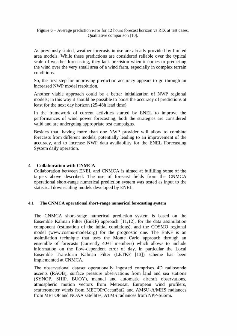
Figure 6 – Average prediction error for 12 hours forecast horizon vs RIX at test cases.
Qualitative comparison [10].
As previously stated, weather forecasts in use are already provided by limited
area models. While these predictions are considered reliable over the typical
scale of weather forecasting, they lack precision when it comes to predicting
the wind over the very small area of a wind farm, especially in complex terrain
conditions.
So, the first step for improving prediction accuracy appears to go through an
increased NWP model resolution.
Another viable approach could be a better initialization of NWP regional
models; in this way it should be possible to boost the accuracy of predictions at
least for the next day horizon (25-48h lead time).
In the framework of current activities started by ENEL to improve the
performances of wind power forecasting, both the strategies are considered
valid and are undergoing appropriate test campaigns.
Besides that, having more than one NWP provider will allow to combine
forecasts from different models, potentially leading to an improvement of the
accuracy, and to increase NWP data availability for the ENEL Forecasting
System daily operation.
4 Collaboration with CNMCA
Collaboration between ENEL and CNMCA is aimed at fulfilling some of the
targets above described. The use of forecast fields from the CNMCA
operational short-range numerical prediction system was tested as input to the
statistical downscaling models developed by ENEL.
4.1 The CNMCA operational short-range numerical forecasting system
The CNMCA short-range numerical prediction system is based on the
Ensemble Kalman Filter (EnKF) approach [11,12], for the data assimilation
component (estimation of the initial conditions), and the COSMO regional
model (www.cosmo-model.org) for the prognostic one. The EnKF is an
assimilation technique that uses the Monte Carlo approach through an
ensemble of forecasts (currently 40+1 members) which allows to include
information on the flow-dependent error of day, in particular the Local
Ensemble Transform Kalman Filter (LETKF [13]) scheme has been
implemented at CNMCA.
The observational dataset operationally ingested comprises 4D radiosonde
ascents (RAOB), surface pressure observations from land and sea stations
(SYNOP, SHIP, BUOY), manual and automatic aircraft observations,
atmospheric motion vectors from Meteosat, European wind profilers,
scatterometer winds from METOP/OceanSat2 and AMSU-A/MHS radiances
from METOP and NOAA satellites, ATMS radiances from NPP-Suomi.

The CNMCA-LETKF data assimilation system is being operationally used
twice a day (00 and 12 UTC runs) to initialize the high-resolution non-
hydrostatic model COSMO integrated up to 72 hours over the Mediterranean-
European region (COSMO-ME, Figure7). The main characteristics of the
CNMCA operational NWP system are:
• The system is running on the Mediterranean-European domain having a
0.0625° grid spacing (7 km) and 40 vertical levels. The configuration is defined
on a rotated regular grid, the coordinates of rotated North Pole are (47.0,-10.0).
Lateral Boundary conditions from IFS (ECMWF-European Center for
Medium-range weather forecasts) deterministic run.
• Figure7: COSMO-ME domain
5 Case study description and results
COSMO-ME forecasts up to 72 hours, starting at 00UTC, over one year period
(that is long enough for wind power purposes), have been provided for testing
by CNMCA. The meteorological data set covers an extended grid centered
over Sicily, where several ENEL Green Power wind farms are located. The
NWP parameters supplied for this test case were wind speed, wind direction,
temperature, pressure and Pasquill stability class, but only the first two have
been used at this preliminary stage. Time series covered the whole year 2012
and were available for 12 lower vertical levels for each one of the grid points.

Figure8– Grid areas, extension and position for COSMO-ME and reference model
NWP data from an internal reference model was adopted as benchmark for this
analysis, while a time series of registered power values from metering system
was used to train the models and to evaluate the prediction errors.
The model chosen here, for an easy preliminary evaluation, was the simple
metering-based neural network described before.
The analysis was carried out for six wind farms (hereinafter referred to with
Test Site 1, Test Site 2, etc.) so that reliable results could be obtained.
NWP models under test were evaluated for the same day prediction (forecast
horizon: 1-24 hours ahead) and for the day-ahead prediction (forecast horizon:
25-48 hours ahead). The two grids for NWP data did not exactly overlap but a
sufficient number of grid points were nevertheless available for a first
performance comparison. NWP data, in either case, were available for the
aforementioned 12 vertical levels whose heights are comprehended
approximately between 0 and 1200 m above ground level.
The first eight months of NWP data were used to train the neural models,
leaving the last four for the testing phase. ANN models were trained and
evaluated in the same conditions for both the NWP data time series.
Results for the intraday prediction are summarized in Table 1 and plotted in
Figure 9.
Table 1 – Performance comparison for intraday prediction (training 1 Jan – 31 Aug,
testing 1 Sep-31 Dec 2012)
Reference [%] COSMO-ME [%]
NMAE CORR NMAE CORR
COSMO-ME
Reference Model

Test Site 1 13.70 0.70 11.78 0.78
Test Site 2 12.15 0.78 10.59 0.81
Test Site 3 9.82 0.79 8.60 0.83
Test Site 4 11.08 0.81 9.49 0.85
Test Site 5 8.80 0.75 7.64 0.80
Test Site 6 11.82 0.76 10.11 0.81
As shown in the table above, COSMO-ME performs very well for all plants.
NMAE is always lower and correlation is steadily higher compared to the
values obtained for the reference model.
Figure9– NMAE% comparison for the intraday prediction
Results for the next day prediction, reported in Table 2 and Figure 10, seem to
get worse compared to the first ones.
Table 2 – Performance comparison for the next day prediction (training 1 Jan – 31
Aug, testing 1 Sep-31 Dec 2012)
Reference [%] COSMO-ME [%]
NMAE CORR NMAE CORR
Test Site 1 14.19 0.68 13.70 0.72
Test Site 2 12.53 0.74 11.92 0.79
Test Site 3 9.80 0.78 9.78 0.80
Test Site 4 11.25 0.79 11.42 0.80
0,00
2,00
4,00
6,00
8,00
10,00
12,00
14,00
T.S.1 T.S.2 T.S.3 T.S.4 T.S.5 T.S.6
NM
AE
%
COSMO-ME Reference

Test Site 5 8.66 0.77 8.75 0.77
Test Site 6 12.01 0.74 11.54 0.77
Prediction errors, as expected on a longer time horizon, increase for both the
reference and COSMO-ME models, but while this growth is minimal and in
some cases negligible for the reference model, it shows a rise for COSMO-ME.
The observed behaviour can be explained considering the differences between
the compared models. COSMO-ME and the reference model are both area
limited models covering the Euro-Mediterranean region, using the same
boundary condition from ECMWF-IFS forecasting system. While the
numerical core of the models is quite similar, the main difference is the
definition of the initial conditions (analysis field): the reference model
estimates initial conditions using a method based on Newtonian relaxation
(nudging of observations), while the COSMO-ME is initialized by an analysis
evaluated through a new method based on the ensemble Kalman filter
algorithm (LETKF), that has been proved to perform better than some
traditional methods (3DVAR). Moreover in a regional model of such
dimensions, the signal coming from the boundary conditions has impact on the
forecast starting from the second day, while in the first day of prediction the
quality of the initial conditions drives the quality of forecasted field. Because
of these considerations it can be concluded that the COSMO-ME model is
expecting to perform better at day one because of the better analysis
evaluation, while at day two the performances of the two models should be
similar because the effects of boundary conditions becomes more important. It
can be also observed that the better quality of COSMO-ME forecast is
depending on the use of a state-of-the-art data assimilation scheme (LETKF
algorithm). The CNMCA is using the new method with encouraging results
since 2011. At that time the choice to move from 3DVAR to LETKF algorithm
has been pioneering, being the CNMCA the first center using operationally an
ensemble-based data assimilation system at regional scale.

Figure10– NMAE% comparison for the next-day prediction
Another analysis can be carried out in order to compare the performances
between the COSMO-ME model and the reference one, regarding the
unbalanced volumes of energy.
In order to estimate these unbalanced volumes of energy, the unbalancing
index IS can be introduced.
This index represents the percentage of the unbalanced volumes of energy
above the franchise level, in respect to the predicted energy.
Herebelow the calculations necessary to obtain this index are shown:
Em = hourly produced energy;
Ep = hourly predicted energy (corrected with the unavailability);
FR = franchise level (0% - 10% - 20%)
On an hourly basis, the following parameters have to be calculated:
EABS = |Em-Ep|
VOL_BURDEN = If ( EABS>FR*Ep) Then ( EABS – FR*Ep ) Else
(0)
Therefore the unbalancing index IS is calculated as follows:
where the summation is extended to the whole analysis period.
0,00
2,00
4,00
6,00
8,00
10,00
12,00
14,00
T.S.1 T.S.2 T.S.3 T.S.4 T.S.5 T.S.6
NM
AE
%
COSMO-ME Reference
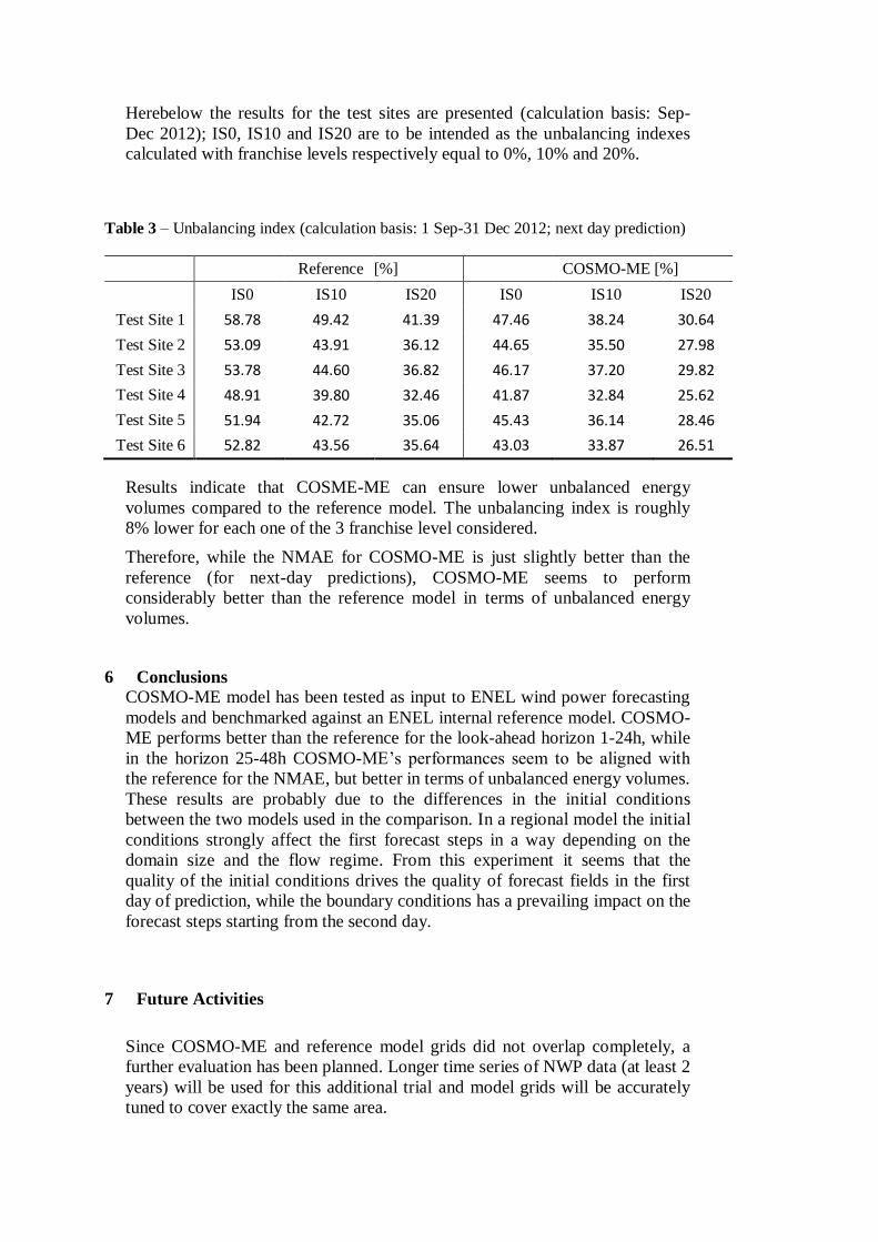
Herebelow the results for the test sites are presented (calculation basis: Sep-
Dec 2012); IS0, IS10 and IS20 are to be intended as the unbalancing indexes
calculated with franchise levels respectively equal to 0%, 10% and 20%.
Table 3 – Unbalancing index (calculation basis: 1 Sep-31 Dec 2012; next day prediction)
Reference [%] COSMO-ME [%]
IS0 IS10 IS20 IS0 IS10 IS20
Test Site 1 58.78 49.42 41.39 47.46 38.24 30.64
Test Site 2 53.09 43.91 36.12 44.65 35.50 27.98
Test Site 3 53.78 44.60 36.82 46.17 37.20 29.82
Test Site 4 48.91 39.80 32.46 41.87 32.84 25.62
Test Site 5 51.94 42.72 35.06 45.43 36.14 28.46
Test Site 6 52.82 43.56 35.64 43.03 33.87 26.51
Results indicate that COSME-ME can ensure lower unbalanced energy
volumes compared to the reference model. The unbalancing index is roughly
8% lower for each one of the 3 franchise level considered.
Therefore, while the NMAE for COSMO-ME is just slightly better than the
reference (for next-day predictions), COSMO-ME seems to perform
considerably better than the reference model in terms of unbalanced energy
volumes.
6 Conclusions
COSMO-ME model has been tested as input to ENEL wind power forecasting
models and benchmarked against an ENEL internal reference model. COSMO-
ME performs better than the reference for the look-ahead horizon 1-24h, while
in the horizon 25-48h COSMO-ME’s performances seem to be aligned with
the reference for the NMAE, but better in terms of unbalanced energy volumes.
These results are probably due to the differences in the initial conditions
between the two models used in the comparison. In a regional model the initial
conditions strongly affect the first forecast steps in a way depending on the
domain size and the flow regime. From this experiment it seems that the
quality of the initial conditions drives the quality of forecast fields in the first
day of prediction, while the boundary conditions has a prevailing impact on the
forecast steps starting from the second day.
7 Future Activities
Since COSMO-ME and reference model grids did not overlap completely, a
further evaluation has been planned. Longer time series of NWP data (at least 2
years) will be used for this additional trial and model grids will be accurately
tuned to cover exactly the same area.

Some investigations will be carried out also for the look-ahead time horizon
49-72h.
Enel is also planning to develop new forecasting models, with different
mesoscale models as input.
8 References [1] Giebel G. et al. (2011). The State-Of-The-Art in Short-Term Prediction of Wind Power: A Literature Overview,
2nd edition. ANEMOS.plus. [2] PetersenE.L. et al. (1998). Wind Power Meteorology. Part I: Climate and Turbulence. Wind Energy, 1, 2-22
(1998) [3] PetersenE.L. et al. (1998). Wind Power Meteorology. Part II: Siting and Models. Wind Energy, 1, 55-72 (1998) [4] Ranaboldo M. (2013)Multiple Linear Regression Mos For Short-term Wind Power Forecast.Lambert Academic
Publishing AG & Co. KG [5] Louka P. et al. (2008).Improvements in wind speed forecasts for wind power prediction purposes using Kalman
filtering. Journal of Wind Engineering and Industrial Aerodynamics, 96(12). DOI:10.1016/j.jweia.2008.03.013 [6] C. Monteiro et al. (2009).Wind Power Forecasting: State-of-the-Art. Argonne National Laboratory, U.S.
Department of Energy.http://www.osti.gov/bridge [7] Z. Liu, W. Gao, Y.-H. Wan and E. Muljadi (2012). Wind Power Plant Prediction by Using Neural Networks.
Conference Paper. IEEE Energy Conversion Conference and Exposition.Raleigh, North Carolina. September 15–20, 2012
[8] Junhui Huang et al. Wind Energy Forecasting: A Review of State-of-the-Art and Recommendations for Better Forecasts. Final Report California Renewable Energy Forecasting, Resource Data and Mapping
[9] Rodrigues A. et al. EPREV - A wind power forecasting tool for Portugal. European Wind Energy Conference and Exhibition 2007, EWEC 2007
[10] Giebel G, Kariniotakis G. Best Practice in Short-Term Forecasting. A Users Guide. Reference to the ANEMOS project, http://www.anemos-project.eu
[11] Bonavita M, Torrisi L, Marcucci F. “The ensemble Kalman filter in an operational regional NWP system:
Preliminary results with real observations”, Q. J. R. Meteorol. Soc., 134, 1733-1744, 2008
[12]Bonavita M, Torrisi L, Marcucci F. “Ensemble data assimilation with the CNMCA regional forecasting system”,
Q. J. R. Meteorol. Soc., 136, 132-145, 2010 [13] Hunt, B. R., E. Kostelich, I. Szunyogh, 2007: Efficient data assimilation for spatiotemporal chaos: a local ensemble transform Kalman filter. Physica D, 230, 112-126
Top Related