


Languages
Pages
Legal


Florida International UniversityFIU Digital Commons
FIU Electronic Theses and Dissertations University Graduate School
6-12-2014
Analysis of Kepler Active Galactic Nuclei Using ARevised Kirk, Rieger, Mastichiadis (1998) ModelSarah M. DhallaFlorida International University, [email protected]
Follow this and additional works at: http://digitalcommons.fiu.edu/etd
This work is brought to you for free and open access by the University Graduate School at FIU Digital Commons. It has been accepted for inclusion inFIU Electronic Theses and Dissertations by an authorized administrator of FIU Digital Commons. For more information, please contact [email protected].
Recommended CitationDhalla, Sarah M., "Analysis of Kepler Active Galactic Nuclei Using A Revised Kirk, Rieger, Mastichiadis (1998) Model" (2014). FIUElectronic Theses and Dissertations. Paper 1521.http://digitalcommons.fiu.edu/etd/1521

FLORIDA INTERNATIONAL UNIVERSITY
Miami, Florida
ANALYSIS OF KEPLER ACTIVE GALACTIC NUCLEI USING A REVISED KIRK,
RIEGER, MASTICHIADIS (1998) JET MODEL
A thesis submitted in partial fulfillment of the
requirements for the degree of
MASTER OF SCIENCE
in
PHYSICS
by
Sarah Mohammed Dhalla
2014

To: Interim Dean Michael R. HeithausCollege of Arts and Sciences
This thesis, written by Sarah Mohammed Dhalla, and entitled Analysis of Kepler ActiveGalactic Nuclei Using a Revised Kirk, Rieger, & Mastichiadis (1998) Jet Model, havingbeen approved in respect to style and intellectual content, is referred to you for judgment.
We have read this thesis and recommend that it be approved.
Caroline Simpson
Walter Van Hamme
James R. Webb, Major Professor
Date of Defense: June 12, 2014
The thesis of Sarah Mohammed Dhalla is approved.
Interim Dean Michael R. HeithausCollege of Arts and Sciences
Dean Lakshmi N. ReddiUniversity Graduate School
Florida International University, 2014
ii

© Copyright 2014 by Sarah Mohammed Dhalla
All rights reserved.
iii

DEDICATION
To my family
iv

ACKNOWLEDGMENTS
A big thanks to my advisor and my committee members for helping me through this
process.
This paper includes data collected by the Kepler mission. Funding for the Kepler mission
is provided by the NASA Science Mission directorate.
v

ABSTRACT OF THE THESIS
ANALYSIS OF KEPLER ACTIVE GALACTIC NUCLEI USING A REVISED KIRK,
RIEGER,& MASTICHIADIS (1988) JET MODEL
by
Sarah Mohammed Dhalla
Florida International University, 2014
Miami, Florida
Professor James R. Webb, Major Professor
Active Galactic Nuclei (AGN) are cores of distant protogalaxies, with a supermassive
blackhole at the center surrounded by an accretion disk, and bipolar jets. Blazars, a subset
of AGN, have their jets aligned with our line of sight. Emission from blazars is highly
variable on all timescales and frequencies. Microvariabilityrefers to rapid continuum
variations that arise within the jet. Bhatta et al. (2013) suggest a modified Kirk, Rieger, &
Mastichiadis (1998) model (KRM) to explain microvariability. The KRM model assumes
that when shock waves passes though the jet, each turbulent cell encountered produces
a pulse of emission characterized by cell size, local density enhancement, and magnetic
field strength. NASA’s Kepler has monitored optical emission from four AGN. We use the
modified KRM model to analyze micro-variations in these Kepler data. The distribution
of cell sizes computed from these data is consistent with the distribution expected from a
turbulent plasma.
vi

TABLE OF CONTENTS
CHAPTER PAGE
1 Introduction 11.1 Active Galactic Nuclei (AGN) . . . . . . . . . . . . . . . . . . . . . . . . 11.2 History of AGN . . . . . . . . . . . . . . . . . . . . . . . . . . . . . . . . 21.3 AGN Classification . . . . . . . . . . . . . . . . . . . . . . . . . . . . . . 31.4 Blazar Variability . . . . . . . . . . . . . . . . . . . . . . . . . . . . . . . 5
2 Modeling Microvariability 82.1 AGN Jets . . . . . . . . . . . . . . . . . . . . . . . . . . . . . . . . . . . 82.2 Model . . . . . . . . . . . . . . . . . . . . . . . . . . . . . . . . . . . . . 92.3 Revised KRM Model . . . . . . . . . . . . . . . . . . . . . . . . . . . . . 102.4 Previous Data . . . . . . . . . . . . . . . . . . . . . . . . . . . . . . . . . 16
3 Multi-color Study of 0716+71 19
4 The Kepler Mission 234.1 Kepler Space Telescope . . . . . . . . . . . . . . . . . . . . . . . . . . . . 234.2 Kepler Data Pipeline . . . . . . . . . . . . . . . . . . . . . . . . . . . . . 26
5 Data Analysis 295.1 Pulse Fitting . . . . . . . . . . . . . . . . . . . . . . . . . . . . . . . . . . 29
5.1.1 Zw 229-15 . . . . . . . . . . . . . . . . . . . . . . . . . . . . . . 335.1.2 KA 1925+50 . . . . . . . . . . . . . . . . . . . . . . . . . . . . . 335.1.3 KA 1858+48 . . . . . . . . . . . . . . . . . . . . . . . . . . . . . 335.1.4 KA 1904+37 . . . . . . . . . . . . . . . . . . . . . . . . . . . . . 34
6 Conclusion and Future Work 44
List of References 41
Appendices 43
vii

LIST OF TABLES
TABLE PAGE
1 WEBT Campaign Data . . . . . . . . . . . . . . . . . . . . . . . . . . . . 16
2 Kepler AGN Source Information . . . . . . . . . . . . . . . . . . . . . . . 27
3 Pulse Fitting Data . . . . . . . . . . . . . . . . . . . . . . . . . . . . . . . 29
4 Zw 229-15 Pulse Fitting Data- Cadence 6 . . . . . . . . . . . . . . . . . . 50
5 Zw 229-15 Pulse Fitting Data- Cadence 7 . . . . . . . . . . . . . . . . . . 51
6 KA 1858+48 Pulse Fitting Data- Cadence 6 . . . . . . . . . . . . . . . . . 53
7 KA 1858+48 Pulse Fitting Data- Cadence 7 . . . . . . . . . . . . . . . . . 55
8 KA 1925+50 Pulse Fitting Data- Cadence 6 . . . . . . . . . . . . . . . . . 57
9 KA 1925+50 Pulse Fitting Data- Cadence 7 . . . . . . . . . . . . . . . . . 60
10 KA 1904+37 Pulse Fitting Data- Cadence 7 . . . . . . . . . . . . . . . . . 62
viii

LIST OF FIGURES
FIGURE PAGE
1 A model of AGN by Urry and Padovani . . . . . . . . . . . . . . . . . . . 2
2 Classifications of AGN depending on their observational angle. . . . . . . . 4
3 A model of a turbulent jet . . . . . . . . . . . . . . . . . . . . . . . . . . . 9
4 Revised KRM model . . . . . . . . . . . . . . . . . . . . . . . . . . . . . 10
5 Pulse shapes for two different frequencies . . . . . . . . . . . . . . . . . . 14
6 Clockwise hysteresis loop . . . . . . . . . . . . . . . . . . . . . . . . . . . 15
7 Counter-Clockwise hysteresis loop . . . . . . . . . . . . . . . . . . . . . . 15
8 Results of the 2009 WEBT Campaign . . . . . . . . . . . . . . . . . . . . 17
9 V band light curve of 0716+71 fitted with 7 pulses . . . . . . . . . . . . . . 18
10 I band light curve of 0716+71, fitted with 8 pulses . . . . . . . . . . . . . . 19
11 Spectral index vs. V band flux . . . . . . . . . . . . . . . . . . . . . . . . 20
12 V (green) and I (red) band pulse shape . . . . . . . . . . . . . . . . . . . . 20
13 Kepler’s field of view, centered in the constellation Lyra and Cygnus . . . . 22
14 Kepler spacecraft . . . . . . . . . . . . . . . . . . . . . . . . . . . . . . . 23
15 Sample light curve of Zw 229-15 . . . . . . . . . . . . . . . . . . . . . . . 25
16 SAP (red) and PDC SAP (blue) light curves . . . . . . . . . . . . . . . . . 25
17 Shape of the Kepler pulse (frequency=575 nm) . . . . . . . . . . . . . . . 27
18 Zw 229-15 cadence 6 fitted light curve . . . . . . . . . . . . . . . . . . . . 32
19 Zw 229-15 cadence 7 fitted light curve . . . . . . . . . . . . . . . . . . . . 32
20 Zw 229-15 cadence 6 and 7 frequency distribution of cell size . . . . . . . . 33
21 KA 1925+50 cadence 6 fitted light curve . . . . . . . . . . . . . . . . . . . 34
22 KA 1925+50 cadence 7 fitted light curve . . . . . . . . . . . . . . . . . . . 34
ix

23 KA 1925+50 cadence 6 and 7 frequency distribution of cell size . . . . . . 35
24 KA 1858+48 cadence 6 fitted light curve . . . . . . . . . . . . . . . . . . . 36
25 KA 1858+48 cadence 7 fitted light curve . . . . . . . . . . . . . . . . . . . 36
26 KA 1858+48 cadence 6 and 7 frequency distribution of cell size . . . . . . 37
27 KA 1904+37 cadence 7 fitted light curve . . . . . . . . . . . . . . . . . . . 37
28 KA 1904+37 cadence 7 frequency distribution of cell size . . . . . . . . . . 38
x

1. Introduction
1.1. Active Galactic Nuclei (AGN)
Active Galactic Nuclei (AGN) are the extremely luminous and unresolved cores of
distant galaxies. Current AGN models propose a Super Massive Black Hole (SMBH) as
the central engine surrounded by an accretion disk. This accretion disk is thought to supply
the SMBH by the injection of matter and magnetic fields. Some AGN are strong sources
of radio emission (radio-loud quasars). These AGN generally have bipolar jet outflows
that extend from the central core of the SMBH and move outwards at relativistic speeds
(0.95c to 0.99c) to a few kiloparsecs (kpc) from the central core. Figure 1 illustrates the
AGN model from Urry & Padovani (1995). Compared to a typical galaxy, AGN have 102
to 104 times the power output with luminosities ranging from a reported 1042 erg/s to 1048
erg/s. However, because some of the AGN cores are obscured by dust and others may be
affected by relativistic beaming, these cores may be much more luminous than reported.
When viewed in the optical, AGN cores appear as unresolved point sources with angular
sizes of much less than 1 arcsec (00).
A key property of AGN is flux variability. Flux variability is observed in all
frequencies and on all timescales. Observations across the electromagnetic spectrum
show that the amplitude of these variations is dependent on frequency. For example,
high amplitude optical variability is often associated with a compact radio structure and
strong high energy �-ray emission. The emission is also linearly polarized because of
synchrotron radiation, thus distinguishing the AGN from stars and galaxies.
Many AGN also have spectra that are characterized by broad optical emission lines,
which is unlike any typical galaxy. Galaxies generally show a thermal spectrum with
stellar absorption lines. The QSO broad emission lines are thought to originate from thick
clouds that are near the central region and are known as the Broad-Line emission Region
1

Fig. 1.— AGN model by Urry and Padovani (1995) illustrating the components of AGNwhich consist of the central engine, accretion disk and bipolar jets.1
(BLR). Narrow lines in the AGN spectra emanate from a thick cloud that encloses the
central broad line region. The BLR region consists of relatively low density clouds several
kpc away from the central engine. In fact it is because of their unique spectra that AGN
were actually first identified as new objects in the universe.
1.2. History of AGN
In 1960 Allan Sandage obtained a photograph of radio source 3C 48 which showed a
faint nebulosity surrounding a stellar object. The spectrum showed broad emission lines
at unfamiliar wavelengths and photometry showed that the stellar-like emission was also
1http://heasarc.gsfc.nasa.gov/docs/cgro/images/epo/gallery/agns/index.html
2

variable with an excess of ultraviolet emission. Several other objects similar to 3C 48 were
found and named quasi-stellar radio sources (QSRS/QSO) or quasars. Allan et al. (1962)
found that 3C 273 consisted of two components: the underlying nucleus and a bright radio
jet emanating from a stellar, point-like source. Maarten Schmidt in 1963 was pondering
the optical spectrum of quasar 3C 273 and found that the emission lines at unfamiliar
wavelengths were actually the Balmer series of hydrogen with a redshift of z=0.158
(Schmidt 1963). He conjectured that the extreme redshift was the result of cosmological
expansion (receding at a rate of 47,000 km/s). This made 3C 273 an extremely distant
object.
During the same time, Cuno Hoffmeister discovered and observed a variable star
named BL Lacertae (BL Lac). Later, MacLeod and Andrew (1968) associated a radio
source with BL Lac. BL Lacertae’s flat spectrum had no emission or absorption lines.
Later, in the 1970s, BL Lac demonstrated the same radio characteristics as other AGN
and because the spectral and radio observations showed that BL Lac behaved similarly to
many AGN, but lacked broad emission lines, it was classified as separate type of AGN.
These different classifications are described below.
1.3. AGN Classification
Active galactic nuclei are classified by many properties that they exhibit. Since there
is no one universal classification system, some AGN may fall into two or more categories
based on their observed properties. In general, they are classified on the basis of their
radio, optical or �-ray emission. An attempt to reconcile this with a physical picture led
to the model where you see different AGN depending on the observed angle to the line of
sight (see Figure 2).
In the viewing angle classification system, Seyfert galaxies are a class of AGN that
are observed at an angle of 0� to 30� with respect to the disk. They were originally divided
3

Fig. 2.— Classifications of AGN depending on their observational angle (Torres 2004).2
into two subclasses: Seyfert I and Seyfert II galaxies. Seyfert I galaxies have luminous
nuclei and have strong emission in the blue optical continuum. They also have broad and
narrow emission lines and are radio quiet. Furthermore, their narrow emission lines show
high ionization. Seyfert II galaxies differ from Seyfert I galaxies in that they have weak
emission lines and sometimes no blue optical continuum and only narrow emission lines
are visible. Radio loud quasars make up another group of AGN and can be subdivided
into broad line radio galaxies (BLRG) and narrow line radio galaxies (NLRG). Broad line
radio galaxies are similar to Seyfert I galaxies and NLRG are similar to Seyfert II galaxies
except that in both cases they are radio loud.
Another class of AGN is the QSO which combines objects such as BL Lac (and other
similar objects) and optically violent variable (OVV) quasars. These objects are at an
observational angle of nearly 0� with respect to the jet, making the host galaxy difficult to
2http://ned.ipac.caltech.edu/level5/March04/Torres/Torres2 4.html
4

image. Steep spectrum QSOs show strong extended emission much more frequently than
do flat spectrum QSOs. BL Lacertae objects show neither broad nor narrow emission lines.
Their optical spectra show highly polarized continuum, are highly variable, exhibit strong
radio emission and emit in the X-ray spectral region. OVV quasars show variability like
BL Lac objects but otherwise have a normal QSO spectrum. Their continuum emission is
highly variable and is thought to originate in a relativistic jet orientated close to the line of
sight. BL Lac objects can be further classified as high-frequency BL Lac objects (HBL)
and low-frequency BL Lac objects (LBL) on the basis of how much energy is contained in
the peaks of their spectral energy distributions (SEDs). Blazars are the combined group of
BL Lac objects and OVV quasars whose flux variability properties are described in detail
in section 1.4.
1.4. Blazar Variability
Blazars include flat spectrum radio quasars (FSRQs) and BL Lac objects. Blazars
have rapid high amplitude flux variability throughout the electromagnetic spectrum on
all time scales, highly variable polarization, large beaming factors and high luminosities.
The spectral energy distribution of blazars is usually a double peaked curve in which
the low energy peak falls between the radio and x-ray region and the high energy peak
falls in the �-ray region. The low energy peak is attributed to the relativistic electrons
in the jet producing synchrotron emission, whereas the high energy peak is attributed
inverse-Compton emission due to the up-scatter of either the synchrotron photons or
external photons by the relativistic electrons.
Initially the best models to explain relativistic jets were the synchrotron self-Compton
(SSC) models (Marscher & Gear 1985; Ghisellini & Maraschi 1989). These models
claim that the synchrotron mechanism produces the smooth, polarized and variable low
energy continuum of blazar spectra whereas the Comptonization of synchrotron radiation
5

is responsible for the high energy component. The Energetic Gamma Ray Experiment
Telescope (EGRET) aboard the Compton Gamma Ray Observatory, discovered very high
and rapid variable MeV-GeV fluxes in many OVV quasars that exceeded synchrotron
fluxes by factors of 10 or more (von Montigny et al. 1995). Thus an external photon field
from either the accretion disk or broadline emission clouds might supply the scattered
photons.
As previously stated, a characteristic of blazars is that their continuum emission is
highly variable. This variability can be sub-categorized as long-term variability, short-term
variability and microvariability. Long-term variability refers to variations that occur on
timescales of months to years. Short-term variability refers to variations on timescales
of weeks to months and microvariability refers to variations that occur on timescales of
minutes to hours. Each type of variability gives insight into the specific physical processes
in the jet and disk. For example, long-term variability is most likely the result of changing
accretion rates onto the black hole, short-term variability to major shock wave events
that occur in the jet, and microvariability to the inhomogeneity and turbulence within the
jet (Marscher 2005). Since the jet of the blazar is closely aligned to the line of sight,
the non-thermal radiation from the jet dominates the radiation from the accretion disk.
Thus we assume that the variations are associated with physical processes in the jet,
not in the disk. It is important to note that the variations seen in blazars are intrinsic
and independent of location or atmospheric effects. It was shown that two telescopes at
different locations, and with different CCD cameras and observing conditions, observe the
same microvariations. (Pollock et al. 2007).
Short-term continuum variability could be due to particle acceleration in the blazar jet.
Particle injection and particle acceleration at the base of the relativistic jet is often thought
to be the cause of rapid variability at high energies (GeV-TeV). In this case, the radiation
and kinetic energy of the particles are converted from the kinetic and internal energy of
the jet itself. Another widely used model of particle acceleration in jets explains high
6

amplitude short term flares by collisions of inhomogeneities ejected by the central engine
with different bulk Lorentz factors and different velocities down the jet (Sikora, Begelman,
& Rees 1994). The collisions accelerate the particles and heat the electrons to medium
energies which are then accelerated relativistically by shockwaves. “Microvariability”
refers to low amplitude, extremely rapid continuum variations that must occur within the
jet. The next section and the remainder of this thesis concentrates on models for these
rapid microvariations.
7

2. Modeling Microvariability
2.1. AGN Jets
As stated previously, the current model of most radio-loud AGNs consists of bipolar
jets emanating from the central black hole. These jets can appear to be short or long,
straight or curved, smooth or knotted and extend to several kilo-parsecs from the central
core. These jets deposit power into the surrounding lobes (observed at radio wavelengths)
(Begelman, Blanford, & Rees 1984). Since the jets in blazars are viewed with nearly a 0�
viewing angle, beaming effects are strong and can therefore distort apparent geometry and
show superluminal apparent speeds.
The jets are accelerated by differential rotation of the polodial component of the
magnetic field in the ergosphere, or in the inner disk. The twisting magnetic fields
emanating from the ergospehere most likely aid in collimating the jets (Meier, Koide, &
Uchida 2000). Active galactic nuclei variability is seen over the entire electromagnetic
spectrum, and the intensities of the variations are amplified by relativistic beaming.
To estimate the amount of energy in the jet, assumptions regarding the intensity of the
magnetic field and amount of relativistic beaming in the jet must be made. The simplest
assumption is that the energies are equally partitioned between the magnetic field and
particle energy density.
Although the source is unresolved at high energies, we can resolve the compact radio
knots that are synchrotron self-absorbed. This allows us to calculate the energy density
in the magnetic field and the energy density in the radiating electrons separately. Perhaps
the dominant process by which particles are injected into the base of the jet is through
pair creation (Meier, Koide, & Uchida 2000). Photons in the ergosphere of the central
blackhole and accretion disk enter the jet and pair-create off the magnetic field.
8

2.2. Model
To better understand the processes occurring in these jets we can try to model the
continuum radiation and variations seen in blazars. In the present thesis we consider the
shock-in-jet model to explain the optical variability properties seen in blazars. This model
involves a shock passing though the jet and accelerating electrons to high energies. The
shockwaves also compress the magnetic field, amplifying it, and the particles cool by
interacting with the magnetic field and emitting synchrotron radiation. Marscher & Gear
(1985) tried to explain superluminal knots seen in radio wavelengths and X-ray variability
observed in 3C 273 by claiming that they arise from shock waves passing through an
adiabatic conical, relativistic jet. According to Sikora et al. (2001) these individual shock
events are caused by velocity irregularities. Sokolov et al. (2004) claimed that the flares
were a consequence of the collision of relativistic shocks with some stationary structures
such as a Mach disk. A diagram of a turbulent jet from Marscher & Gear (1985) is shown
in Figure 3.
Fig. 3.— A model of a turbulent jet by Marscher & Gear (1985).
As the shockwave travels through the turbulent plasma it excites individual cells,
which then emit a pulse of synchrotron emission. The amplitude and shape of the pulse
depends on the size of the cell, magnetic field and local density enhancement. However
we note that if the flow of the plasma is laminar, there are no individual cells and we will
see a flare but not microvariability (Bhatta et al. 2013).
9

2.3. Revised KRM Model
To describe a short term flare seen in Mkn 501, Kirk, Rieger, & Mastichiadis (1998)
(hereafter KRM) modeled a shock wave passing through a cylindrical jet and interacting
with a density-enhanced region of uniform magnetic field. The KRM model states that
electrons are accelerated and emit synchrotron radiation as they cool. The duration of the
pulse is therefore related to the size of the density-enhanced region. By revising this model
slightly we can describe the microvariations seen in blazars. Instead of considering just
one density-enhanced region as the KRM model did, we consider several density-enhanced
regions modeled as cylindrical cells (see Figure 4).
Fig. 4.— Revised KRM Model: Turbulent cells are modeled as cylinders filling the plasmajet. Cells of higher density are bluer and cells of lower density are redder. The shock frontis shown as moving from left to right.
As the shock wave hits each individual cell, a pulse is generated whose duration
is dependent on the size of the cell and whose amplitude depends on the density
enhancement. To mathematically describe the KRM model, as done in Kirk, Rieger &
Mastichiadis (1998), we consider two regions of each cell: the acceleration zone and the
emission zone. We consider the frame in which the plasma is at rest in the jet frame.
10

The acceleration region is considered to be very small and occurs at the shock front
which is modeled as a delta function. The diffusion equation in 2.1 describes the electron
distribution when a plane shock wave hits electrons with energy �0 in the acceleration
zone. The electrons are accelerated to a maximum energy �
max
.
@N
@t
+@
@�
✓�
t
acc
� �
s
�
2
◆�N +
N
t
acc
= Q�(� � �0). (2.1)
The first term on the left describes the change in number of particles N, at a specific
energy, over time and the third term is the escape term. The second term on the left
(quantity in brackets) contains two terms: the acceleration term and the loss of energy due
to synchrotron radiation, with � given in equation 2.2.
�
s
=4
3
�
T
m
e
c
2
✓B
2
2µ0
◆. (2.2)
The term on the right side describes the particle injection rate. Kirk, Rieger & Mastichiadis
(1998) solved this differential equation using the Laplace transformation method to obtain
the solution:
N(�, t) = a
1
�
2
✓1
�
� 1
�
max
◆(tacc�tesc)/tesc
⇥⇥ (� � �0)⇥ (�1 (t)� �) . (2.3)
This is the solution given certain boundary conditions (�0 < � < �1(t) and N(�,t)=0),
where ⇥ is the Heaviside step functions and a is a constant:
a = Q0tacc�tacc/tesc
0
✓1� �0
�
max
◆�tacc/tesc
. (2.4)
If one considers that the electron begins at some energy �0, then after a certain time t, the
electron may not have reached �
max
, but instead reaches �1(t):
�1(t) =
✓1
�
max
+
1
�0� 1
�
max
�e
�t/tacc
◆�1
. (2.5)
11

As particles are accelerated, they travel downstream in the plasma where they cool by
emitting synchrotron radiation. This therefore is considered to be the emission zone and is
restricted to length L, the maximum extent of the emission region,
L =t
b
u
s
1� u
s
/c
. (2.6)
Just as there was a diffusion equation to describe the particle density in the acceleration
zone, there is a similar equation to describe the particle density in the emission zone,
however this time there is no acceleration term.
@n
@t
� @
@�
��
s
�
2n
�=
N(�, t)
t
esc
� (x� x
s
(t)) . (2.7)
Here n is the number density per unit length for a given energy and x
s
(t) is the position of
the shock front. Following a similar procedure as done in the acceleration zone, if we solve
the differential equation for the emission zone using the Greens synchrotron function,
P (⌫, �) = a
s
z
0.3exp(�z), (2.8)
where a
s
=p3e2⌦sin✓
2⇡c is a constant, and z ⌘ 4⇡⌫/ (3⌦sin✓�2), with ⌦ = eB
m
the electron
gyro frequency, and ✓ the angle between the magnetic field direction and the line of sight,
we get the solution
n (x, �, t) =a
u
s
t
esc
�
2
1
�
� �
s
✓t� x
u
s
◆� 1
�
max
�(tacc�tesc)/tesc
⇥⇥⇥�1 (x/u
s
)� (1/� � �
s
t+ �
s
x/u
s
)�1⇤.
(2.9)
Here we have used boundary conditions such that acceleration begins at x=0 and t=0, and
that the shock moves with constant speed u
s
. This describes the emission at a particular
energy. In order to determine the total intensity of the emission we must first integrate the
12

intensity for a single energy and single time, over the spatial volume.
Zn(x, �, t)dx =
a
(1� usc
)�(tacc+tesc)/tesc(max)
(�
max
�
)2⇢[�
max
�
� t
t
acc
+x(1� u
s
/c)
u
s
t
acc
]tacc/tesc�
x1(t)
x0(�,t)
.
(2.10)
Equation 2.11 is an expression for the synchrotron radiation emitted while the particle is in
the emission zone. However we must also consider the contribution to the intensity given
by the particle while it is in the acceleration zone.
I0 (⌫, t) =
Z ZP (⌫, �)n (x, �, t+ x/c) dxd�. (2.11)
If the magnetic field in front of the shock front was the same as the magnetic field after the
shock front then we can just simply use 2.11. However for the t > t
on
(where t
on
is the
time the shock begins), we have an extra term
I
s
(⌫, t) =
Zd�P (⌫, �)
ZdxN(�, t)�[x� u
s
(t+ x/c)] =
a
(1� usc
)�(tacc+tesc)/tesc(max)
Zd�P (⌫, �)(
�
max
�
)2(�
max
�
� 1)(tacc+tesc)/tesc.
(2.12)
Therefore the total emission would be given by
I (⌫, t) = I0 (⌫, t) + I
s
(⌫, t). (2.13)
If we now would like to model variability we can increase the particle injection rate by a
factor of 1+⌘f
for a time t
f
. We then have that
Q (t) = Q0 for t < 0 and t > t
f
and
Q (t) = (1 + ⌘
f
)Q0 for 0 < t < t
f
.
(2.14)
13

Our total intensity now becomes
I (⌫, t) = I1 (⌫, t) + ⌘
f
[I1 (⌫, t)� I1 (⌫, (1� u
s
/c) tf
)] . (2.15)
We used the computer language IDL by Exelis to write a program to solve the above
equation. The pulse program calculates and plots the shape of the curve (Figure 5)
resulting from the equations above (Bhatta et al. 2013). The pulse program in IDL is
included as Appendix I. As seen in Figure 5, the shape of the pulse is dependent on the
frequency of the emission.
Fig. 5.— Pulse shapes for two different frequencies: ⌫ = 4.3 ⇥ 1016 Hz (blue) and ⌫ =4.3 ⇥ 1017 Hz (red). Input parameters : B=2 Gauss, Q = 609.3 m�3s�1 and time of flaret
f
= 1.25/tacc
.
The size of the cell can then be computed by using the width of the pulse:
cellsize = t
flare
⇥ �c
t
flare
=1
2⇥ pulsewidth .
(2.16)
The model also predicts the behavior of the spectral index as the flare evolves. The
spectral index is a measure of the dependence of flux on frequency. If the information
14

about changes in injection propagates from high to low energies by synchrotron cooling
(or any other cooling method), the spectral index exhibits a clock-wise loop-like pattern
when plotted against the flux at the lower frequency (Figure 6). This pattern has been
observed by several sources in different wavelengths e.g. OJ 287 (Gear et al. 1986), Mkn
421 (Takahashi et al. 1996; Kirk, Rieger & Mastichiadis 1998). If the spectral index
is plotted against the higher frequency observed where cooling and acceleration times
are equal, the loop-like behavior is still present except that the direction is now counter
clock-wise (Figure 7).
Fig. 6.— Clockwise hys-teresis loop produced whenspectral index is plottedagainst flux of lower fre-quency (Kirk, Rieger &Mastichiadis 1998).
Fig. 7.— Counter-Clockwise hysteresis loopproduced when spectral in-dex is plotted against fluxof higher frequency (Kirk,Rieger & Mastichiadis1998).
Before we can quantify luminosities or sizes in the source rest frame, we must
consider that these objects are at a very high red shift and the jet speeds are relativistic, so
relativistic corrections need to be made using a revised Doppler Factor
Correction Factor =z
� (1� �cos')(2.17)
(Kembhavi & Narlikar 1999) where � is the Lorentz bulk factor, � is the velocity, ' is the
angle between the jet and the line of sight and z is the redshift.
15

2.4. Previous Data
The first test to the revised version of the KRM model was done on the 2009 Whole
Earth Blazar Telescope (WEBT) campaign. For this campaign, Bhatta et al. (2013)
collaborated with 36 observatories in 16 countries to create a 78.88 hour light curve of
0716+71. The details of the campaign are listed in Table 1.
The short term and long term trend in the light curves were subtracted so that only
microvariations remained. The location of each pulse was determined to be the center of
each local peak in the data and its amplitude and size were determined by a best fit to
the data. Bhatta et al. (2013) fit 35 pulses to the light curve with a correlation coefficient
of 0.98, showing that the model correctly described the light curve behavior. However
because the WEBT data were only taken in a single filter, the R filter, they were unable to
test the hysteresis loop change in the spectral index.
Rafle et al. (2012) simultaneously conducted a microvariability study to test the KRM
model using data from the long term monitoring campaign of 0716+71 by Montagni et al.
(2006) from 1996-2003. Rafle et al. (2012) fit pulses to 37 individual light curves, each
with an average duration of nine hours. Each light curve had an average of 6.43 pulses
and a maximum and minimum correlation coefficient of 0.997 and 0.85, respectively.
Similarly, the spectral index test was not able to be completed since there were no
simultaneous multi-frequency observations available.
Table 1 WEBT Campaign Data
Time Length of Campaign 78.88 hrsNumber of Data Points 2613Mean Magnitude (R) 13.75Amplitude 0.31Standard Deviation 9.8 %
16

Fig. 8.— Results of the 2009 WEBT Campaign (Bhatta et al. 2013).
In order to verify that the KRM correctly describes the microvariations seen in
blazars, simultaneous multi-frequency observations need to be made in order to determine
if the spectral index changes with time in a hysteresis loop manner predicted by the model.
For this we require simultaneous observations of the same object with two different filters.
The spectral variability analysis is detailed further in chapter 3.
In addition to testing spectral variability, the pulse model needs to be tested on
more than just one object. We have data on several objects taken with the Southeastern
Association for Research in Astronomy3 (SARA) 0.9-m telescope, however these data
posed a few problems. Because the duration of a night is a maximum of about nine hours
and because the uncertainty in the flux was at times large, we were unable to determine
whether the pulses from SARA data were actually one pulse or two convolved pulses.
Another problem is the relatively large error in the SARA data compared to the expected
effect.
3Southeastern Association for Research in Astronomy (http://saraobservatory.org/).
17

3. Multi-color Study of 0716+71
In order to further test the KRM model, we carried out an attempt to test for the
frequency hysteresis predicted by the KRM model. This part of our study focused on
the spectral index analysis of 0716+71. Blazar 0716+71 is a bright BL Lac object with a
redshift of z=0.31 ± 0.08. This object was chosen since it has a duty cycle of about 95.3%,
meaning it is nearly always undergoing microvariability (Webb et al. 2010). Since we only
needed one clearly isolated pulse to produce the expected spectral hysteresis, we were able
to use the SARA 0.9 m telescope located in Kitt Peak, Arizona. The observations were
taken in Johnson & Cousins V and I bands simultaneously. The bands were chosen since
they are the most widely separated of the optical frequency bands to which our cameras
are sensitive. The simultaneous light curves are shown in Figure 9 and 10.
Fig. 9.— V band light curve of 0716+71 fitted with 7 pulses. Data taken on 4/03/13 withSARA 0.9-m telescope.
Finally, spectral variability was plotted against V band flux for one isolated pulse
(Figure 11). Analysis showed there was no smooth hysteresis loop as predicted by the
18

Fig. 10.— I band light curve of 0716+71, fitted with 8 pulses. Data taken on 4/03/13 withSARA 0.9-m telescope.
KRM model, although there was a loop structure (beginning at 9.0 mJy and looping
counter clockwise to 9.12 mJy). Not much confidence can be placed in the loop structure
seen in the data since the error in flux was quite large. Perhaps the bands are not as
separated enough in frequency to produce the spectral variability within error. As seen
in Figure 12, the pulse shape for the V and I bands are not dramatically different. In the
timescale of this thesis, we were unable to gather simultaneous data from two widely
separated frequency bands.
19

Fig. 11.— Spectral index vs. V band flux.
Fig. 12.— V (green) and I (red) band pulse shape.20

4. The Kepler Mission
4.1. Kepler Space Telescope
An additional test of the KRM model is fitting long, continuous and high quality data
sets. In 2010, the Kepler satellite telescope observed four AGN intensively and with high
precision. On March 7th, 2009, NASA launched Kepler into an Earth-trailing heliocentric
orbit. Kepler’s primary mission was to detect transiting Earth-size planets in the habitable
zone of F through M type stars in the constellations Lyra and Cygnus. These data sets
spanned three months each and are excellent candidates for our study. Since Kepler was
trying to detect planetary transits, which only last a fraction of a day, it was important
that the field of view was not blocked during any time of the year. Furthermore, it was
important to have a large number of stars in the field of view (FOV), while at the same
time not be on the galactic plane in order to reduce field confusion. This led to the field
of view being large enough to monitor ⇠ 100,000 stars in the constellations Cygnus and
Lyra (Figure 13). Every quarter, Kepler rolled 90 degrees about its optical axis in order to
keep the sun on the solar panels and keep the radiators pointed to deep space to cool the
focal plane. This meant that although the same area of the sky was observed, a particular
star could be in one of four different parts of the focal plane depending on the season (Van
Cleve et al. 2009).
Kepler has a 0.95-m aperture Schmidt telescope with a 94.6 million pixel CCD
detector array, which contains both the Science and Fine Guidance Sensor (FGS) pixels.
The diameter of the FOV is 115.6 FOV is 115.6 deg2 and is covered with active pixels.
The “frame” is considered the set of pixels collected by one repetition of the CCD
clocking cycle and the integration time is the interval between reads of a given pixel.
Observing periods are defined as “cadences” and are the set of co-added and stored
pixels over a certain amount of time. Kepler collects two main types of cadences:
short cadence and long cadence. The default exposure time for a short cadence is
21

Fig. 13.— Kepler’s field of view, centered in the constellations Lyra and Cygnus (VanCleve et al. 2009).
54.2 seconds whereas the default exposure time for a long cadence is 1626 seconds
(https://archive.stsci.edu/mast faq.php?mission=KEPLER).
Every month, data are downlinked through the High Gain Antenna (HGA) and
processed by the Data Management Center (DMC) and then archived at the Space
Telescope Science Institute (STScI). Data calibration and download is discussed in more
detail in the next section, however it is important to note that Kepler does not download
full images. Furthermore, since Kepler is designed to repeat observations precisely it does
not have many user options. There are no filters or integration parameters that a user
can select and only Kepler magnitudes and counts (e/second) are recorded. Instrument
calibration and long-term operating parameters were fixed during the Commissioning
Phase which was concluded on May 12th, 2009 (Van Cleve et al. 2009).
22

Fig. 14.— Kepler spacecraft (Van Cleve et al. 2009).
Initially Kepler was supposed to last 3.5 years, but as a result of interference from the
spacecraft, additional time was needed to complete the mission. The extended mission was
supposed to last until 2016, however on May 11th, 2013 a second of four gyroscope-like
reaction wheels failed, meaning the current mission needed to be modified. “K2,” also
known as “Second Light”, is a newly proposed plan presented in November 2013. K2
would use Kepler’s remaining capability to collect data on supernovae, young and old
stars, and AGN. The orientation of the spacecraft must be nearly parallel to its orbital path
around the sun to achieve necessary stability. Instead of the four rolls per year as before,
K2 would study a specific portion of the sky for 83 days and turning 4.5 times per year
(http://www.nasa.gov/kepler/keplers-second-light-how-k2-will-work/#.Uz2Z9vldV0Y).
In addition to the 2,740 planetary candidates, Kepler also found 3 new AGN (KA
1904+37, KA 1925+50, KA 1858+48) in its initial phase. These new, serendipitously
discovered AGN happened to lie in the observed field, along with AGN Zw 229-15, and
had well-observed light curves. After it was realized the Kepler had observations of
these four AGN, several analyses of their light curves were conducted which are further
described in section 5.1.
23

4.2. Kepler Data Pipeline
The science pipeline consists of several steps. Once every month, data are transmitted
from the spacecraft to the Mission Operations Center, located at the Laboratory for
Atmospheric and Space Physics (LASP) in Boulder, Colorado and then to the DMC. The
data are then sent to the Kepler Science Operations Center (SOC). The pipeline consists
of several steps and allows for parallel processing of the data. First, raw pixel data are
downlinked to the Calibration module (CAL). This produces calibrated pixels of the target
object and the background. The data are then processed by Photometric Analysis (PA),
which removes sky background and extracts simple aperture photometry. Before a light
curve is created, the data go through Pre-search Data Conditioning (PDC). The pre-search
data conditioning step removes systematic errors such as pointing drift, focus changes, and
thermal transients and is specific to the detection of extra-solar planets (Jenkins 2010).
Kepler has unprecedented data quality with its . 0.1 % repeatability. A sample
light curve of Zw 229-15 is shown with error bars in Figure 15. An independent check
of Kepler data was done by the ground-based Lick AGN Monitoring Campaign (LAMP)
for Zw-229-15. The light curves show very good agreement between Kepler and LAMP
within the 1% errors of LAMP. Kepler errors are however much smaller than LAMP errors
and currently there is no way to be sure that systematic errors are not affecting the data.
There are small short-term discontinuities following monthly downloads that are believed
to be due thermally induced focus changes (Mushotzky et al. 2011).
Two types of flux measurements are recorded, PDC SAP FLUX and SAP FLUX. The
differences between these two measurements lie in the correction factor for some of the
short-term gain effects. Since PDC SAP FLUX count rates are identical to the SAP FLUX
count rates only offset by a constant, the variations are identical in each set (Figure 16).
We use the SAP FLUX rates in our analysis so as not to remove any small variations that
may have been removed by the PDC processing, but are intrinsic to the quasar.
24

1.17
1.18
1.19
1.20
1.21
1.22
1.23
1.24
x104
540
550
560
570
580
590
600
610
620
630
TIM
E / B
JD -
2454
833
SAP_FLUX / e-/s
Fig.
15.—
Sam
ple
light
curv
eof
Zw22
9-15
.Err
orba
rsar
ein
clud
ed,b
utar
eve
rysm
all.
1.17
1.18
1.19
1.20
1.21
1.22
1.23
1.24
1.25
1.26
x104
540
545
550
555
560
565
570
575
580
585
590
595
600
605
610
615
620
625
630
TIM
E / B
JD -
2454
833
SAP_FLUX / e-/s
SAP
FLU
XPD
C S
AP F
LUX
Fig.
16.—
SAP
(red
)and
PDC
SAP
(blu
e)lig
htcu
rves
.
25

5. Data Analysis
5.1. Pulse Fitting
Because Kepler has such large temporal coverage, sampling one point every 30
minutes, and excellent data quality, we are able to use the Kepler data sets to study the
microvariability in the four Kepler AGN (Table 2) in our microvariability study. Because
of the flux discontinuity, these data sets cannot be combined into one large data set,
however each quarter contains 3 months of continuous data which is a factor of 10 longer
than even the WEBT 0716+71 observation.
In this thesis, we have applied the modified KRM jet model to the variations seen in
the Kepler AGN data. Because the Kepler data sets are of such high quality, we can use the
KRM model to analyze the properties of the Kepler AGN jets through the microvariability
pulse analysis. Recall that Kepler has no filters, therefore the “Kepler magnitude” is
defined as the spectral response of the CCD convolved with the color of the target (Van
Cleve et al. 2009). At present, there is no reliable conversion from Kepler magnitudes to
the standard Johnson & Cousins magnitude system used in other light curves. We modeled
the pulse shape based on the peak spectral response of Kepler which is centered on 575
nm. The resulting pulse shape is shown in Figure 17.
In order to fit the pulses to the data, we used the IDL pulse fitting program,
documented in Appendix II. In our model, each pulse corresponds to the shockwave
hitting a density-enhanced region within the jet. By convolving the pulses, we treat the
light curve as a convolution of pulses from the turbulent cells that vary in size, density, and
location within the jet. We take the center of the pulse to be the center of each individual
feature seen in the light curve and then adjust the Full Width Half Max (FWHM) of the
pulse, retaining the shape, to fit the feature.
26

Table 2 Kepler AGN Source Information
Source Name RA (J2000) Dec (J2000) z
Zw 229-15 19 05 26.0 +42 27 40 0.028KA 1925+50 19 25 02.2 +50 43 14 0.067KA 1858+48 18 58 01.1 +48 50 23 0.079KA 1904+37 19 04 58.7 +37 55 41 0.089
Fig. 17.— Shape of the Kepler pulse (frequency=575 nm). Time and Flux units are arbi-trary in this figure.
27

The center of the cell therefore gives us the location of the cell, the amplitude corresponds
to the density enhancement within the cell, and the pulse width to the size of the cell. The
best fit to the data was determined by using a combination of the FWHM and amplitude
that produced the highest correlation coefficient to the data. Cadences 6 and 7 were chosen
for each object (except for KA 1904+37 because no cadence 6 information was available)
for the analysis. Details of the pulses fitted for each object are shown in Appendix III.
Table 3 summarizes the analysis giving the cadence number, number of points in each
data set, number of pulses fit, average cell size (AU), correlation coefficient and degrees
of freedom4. Errors are not noted, however fits were performed until the correlation
coefficient was highest.
4The degrees of freedom are defined as (#points� (#pulses⇥ 3)� 1).
28

Table 3 Pulse Fitting Data
Galaxy Name Cadence Number Number of Average Cell Correlation DegreesName Number of Points Pulses/Cells Size (AU) Coefficient of Freedom
Zw 229-15 6 4276 38 35.83 0.98 41617 4227 42 34.65 0.99 4100
1925+50 6 4277 55 36.70 0.99 41117 4226 52 40.34 0.99 4069
1858+48 6 4277 46 31.34 0.99 41387 4226 37 28.51 0.99 4114
1904+37 7 4227 26 54.70 0.99 4148
29

5.1.1. Zw 229-15
The cadence 6 and 7 light curves for Zw 229-15 are shown in figures 18 and 19. The
cadence 6 light curve had a total of 4,276 points and we fit 38 pulses with a correlation
coefficient of 0.985 and 4161 degrees of freedom. Cadence 7 had a total of 4,227 points
with a total of 42 pulses and a correlation coefficient of 0.99 and 4100 degrees of freedom.
The average cell size for cadence 6 was 35.82 AU and for cadence 7 was 34.65 AU. The
frequency distribution of cell sizes is shown in Figure 20. The figure clearly shows that
most cells are of a smaller size consistent with the distribution of cell sizes expected in a
turbulent plasma.
5.1.2. KA 1925+50
For object KA 1925+50, cadence 6 had a total of 4,277 points and 55 pulses and a
correlation coefficient of 0.99. Similarly, cadence 7 had a total of 4,226 points and 52
pulses total. The average cell size for KA 1925+50 is similar to that of Zw 229-25. Again,
the cell size frequency distribution is consistent with the turbulent plasma assumption
(Figure 23).
5.1.3. KA 1858+48
Fitted light curves for KA 1858+48 cadence 6 and 7 are shown in Figure 24 and 25,
respectively. Again cell sizes seem to be consistent with the first three objects in our study
and the cell size frequency distribution is therefore consistent with the cell size distribution
for a turbulent plasma.
30

5.1.4. KA 1904+37
The last object in our study, KA 1904+37 did not have data during cadence 6 so only
cadence 7 was analyzed. KA 1904+37 had a total of 27 pulses in 4,227 points. The cell
size frequency distribution is similar to the other objects, with most cells ranging 40-60
AU in size.
31

Fig. 18.— Zw 229-15 cadence 6 fitted light curve, where the red lines represent the pulsesand the black, data points.
Fig. 19.— Zw 229-15 cadence 7 fitted light curve, where the red lines represent the pulsesand the black, data points.
32

Fig. 20.— Zw 229-15 cadence 6 and 7 frequency distribution of cell size.
33

Fig. 21.— KA 1925+50 cadence 6 fitted light curve, where the red lines represent thepulses and the black, data points.
Fig. 22.— KA 1925+50 cadence 7 fitted light curve, where the red lines represent thepulses and the black, data points.
34

Fig. 23.— KA 1925+50 cadence 6 and 7 frequency distribution of cell size.
35

Fig. 24.— KA 1858+48 cadence 6 fitted light curve, where the red lines represent thepulses and the black, data points.
Fig. 25.— KA 1858+48 cadence 7 fitted light curve, where the red lines represent thepulses and the black, data points.
36

Fig. 26.— KA 1858+48 cadence 6 and 7 frequency distribution of cell size.
Fig. 27.— KA 1904+37 cadence 7 fitted light curve, where the red lines represent thepulses and the black, data points.
37

Fig. 28.— KA 1904+37 cadence 7 frequency distribution of cell size.
38

6. Conclusion and Future Work
The analysis of Kepler objects using the KRM model showed that the average cell
size for each object was ⇠ 37.4 AU. The WEBT Campaign produced a 78.88 hour light
curve of 0716+78 fitted with 37 pulses. The average cell size was 36.50 AU. When
compared to the light curves in the Kepler study, we see that the average cell sizes are very
similar. Because the cell sizes in all objects (including 0716+71) seem to be similar, we
can assume that the same processes are occurring in these AGN jets. Furthermore, we can
see that there are very few cells that are larger than 60 AU, which further agrees with the
theory that the larger cells in a turbulent plasma may be unstable and break apart.
In order to verify our results, we would like to further study the Kepler objects using
the SARA 0.9 m telescope. Since Kepler does not have standard calibrated magnitudes,
we can observe the objects with multiple filters and perform aperture photometry using
comparison stars in the field to get a baseline calibration for the Kepler observations. By
observing these objects in multiple filters, we can also perform the spectral analysis to
determine if there is a difference between the results found in the 0716+71 spectral study.
With regards to the spectral study of 0716+71, we did not recover the hysteresis loop-like
structure as predicted by Kirk, Rieger & Mastichiadis (1998). Our group is still in the
process of replicating the graphs and code that were presented in their paper. It is possible
that the V and I frequency bands are not separated widely enough. Therefore, in order
to verify the model, our group plans to write a proposal to use the Keck Observatory’s
near-infrared and optical telescopes (located in Mauna Kea, Hawaii) to observe 0716+71
simultaneously. Recall, since we only need one isolated pulse to perform the spectral
study, we hope that we can recover the spectral hysteresis loop as predicted by Kirk,
Rieger & Mastichiadis (1998).
In addition to the proposed observational runs, we also plan to improve the model
to make it more realistic. The current model assumed that all the cells in the jet are
39

cylindrical, therefore we need modify the program to allow for spherical cells. In
addition, we would like to simulate variability using a distribution of cell sizes consistent
with plasma turbulence. Our model also assumes that the magnetic field in the jet is
homogenous and does not vary as a function of jet radius. Our model does not consider
high energy particle processes and only takes into account the synchrotron emission due to
synchrotron radiation and excludes Compton contribution. Furthermore, to make the pulse
fitting process more efficient, we plan to automate the fitting process..
40

List of References
https://archive.stsci.edu/mast faq.php?mission=KEPLER.
http://www.nasa.gov/kepler/keplers-second-light-how-k2-will-work/#.Uz2Z9vldV0Y.
Allen, L.R., Anderson, B., Conway, R.G., et al. 1962, Mon. Not. Roy. Astron. Soc., 142,477.
Begelman, M. C., Blandford, R. D., & Rees, M. J. 1984, Rev. Mod. Phys., 56, 255.
Bhatta G. et al., 2013, A&A, 558, 92.
Gear W.K., Robson E.I., Brown L.M.J. 1986, Nature, 324, 546.
Ghisellini G., & Maraschi L. 1989, ApJ, 340, 181.
Jenkins, J. M., Caldwell, D. A., Chandrasekaran, H., et al. 2010, ApJ, 713, L87.
Khembhavi G. & Narlikar J. 1999, Quasars and Active Galactic Nuclei, CambridgeUniversity Press.
Kirk J.G., Rieger, F.M., & Mastichiadis, M. 1998, A&A, 333, 452.
Marscher, A.P., & Gear, W.K 1985, ApJ, 298, 114.
Marscher, A. 2005, MSAI, 76, 168.
Mc Leod, A., & Andrew, B.H. 1968, Astrophys. Let., 1, 243.
Meier, D. L., Koide, S., & Uchida, Y. 2000, Science, 291, 84.
Montagni, F., Maselli, A., Massaro, E., et al. 2006, A&A, 451, 435.
Mushotzky R. F., Edelson R., Baumgartner W., et al. 2011, ApJ, 743, L12.
Pollock J. T., Webb J. R., & Azarnia G. 2007, AJ, 133, 487.
Rafle, H., Webb, J.R., & Bhatta, G. 2012, jSARA, 7, 33.
41

Schmidt, M., 1963 Nature 197, 1040.
Sikora M., Begelman M.C., & Rees M.J. 1994, ApJ, 421, 153.
Sikora, M., Blazejowski, M., Begelman, M. C., et al. 2001, ApJ, 554, 1; Erratum: ApJ561, 1154 (2001).
Sokolov, A., Marscher, A.P., & McHardy, I.A. 2004, ApJ, 613, 725.
Takahashi T., Tashiro M., Madejski G., et al. 1996, ApJ, 470, L89.
Torres, D.F., 2004 http://ned.ipac.caltech.edu/level5/March04/Torres/Torres2 4.html
Urry, C.M., Padovani, P. 1995, PSAP, 107, 803,http://heasarc.gsfc.nasa.gov/docs/cgro/images/epo/gallery/agns/index.html
Van Cleve, J., Caldwell, D., Thompson, R., et al. 2009, Kepler A Search for TerrestrialPlanets, Document KSCI-19033-001 NASA Ames Research Center, Kepler InstrumentHandbook Manual (Pasadena, CA: SSC), https://archive.stsci.edu/kepler/manuals/KSCI-19033-001.pdf
von Montigny C. et al. 1995, ApJ, 440, 525
Webb, J. R., 2010, BAAS, 21642011W. 14
42

APPENDIX I- Pulse Program (Bhatta et al., 2013) Pro Make pulse, Flare,Tm
COMMON parameters,gama max,gama not,cs,us,tacc ; Common parameters shared by
the program and the function below
;/ constants/
amp=5.0 ; A normalization number of the amplitude of the pulse
B=1.0e-3/amp ; Maganetic field
cs=3.0e+8 ; Speed of light
us=0.1*cs; Speed of shock
rho T= 6.65e-29 ; Thompson scattering constant
m e=9.1e-31 ; Mass of electron
mu 0=!pi*4.0e-7 ; Pearmeability for free space
gama not = 10.0 ; Minimum Lorentz factorof the electrons
gama max=1000.0 ; Maxmimum Lorentz factor of the electrons
beta s = 4.0/3.0*rho T(m e*cs)*(B2̂/(2*mu 0)) ; A constant in the KRM equations
tacc=1/(gama max*beta s) ; accelaration time
tesc=2.0*tacc ; escape time
Q=609.31; A normalise particle injection rate for the back ground intensity and divided by
2 for the fact that the injection is enhanced by a factor of 2
data length=gama max-gama not ; the difference between the maximum and minimun
Lorentz factors of the electrons
data interval=0.5
data nums=data length/data interval
43

power=(tacc-tesc)/tesc
pwr=(tacc+tesc)/tesc
a=Q*tacc*gama not(̂tacc/tesc)*(1-gama not/gama max) ; a constant is equation 2.5
factor = 1/gama not -1/gama max
as=4.1e-36*B
Nu=4.3e14; Optical frequency for the R filter
time=50 ; Time arrry
tm=fltarr(Time)
t m=fltarr(Time)
Flux=fltarr(Time)
Flux2=fltarr(Time)
Intensity=fltarr(Time)
For k=0,Time-1 do begin tm(k)=(k+1.0)*tacc*0.1 ; Time loop
t=tm(k)
x1= t*us/(1-us/cs) ; Position of shock wave front
gama1=1/(1/gama max+factor*exp(-t/tacc)) ; Instantaneous Larentz factor given by the
equation 2.5
;print,”gamma1 is”,gama1
;/This part of the program ensure that incoming gamas are less than
; /gama1
r=gama not+findgen(data nums+1.0)*data interval
;print,r y1=where(r lt gama1,count) ; Finds the total number of elements statisfying the
44

condition
gama=fltarr(count)
gama=r(0:count-1); Creating subarray from r
;print,gama
;/New variables declarations
N=fltarr(count); particle density
sync func=fltlarr(count) ; Green’s synchrotron function given by the equation 2.8
z=fltarr(count) ; A term is the equation 2.8
P=fltarr(count)
F=fltarr(count) ; Flux given by the equation 2.11
;/This part of the program calculates the flux
For i=0,count-1 do begin
;Length=(t-tb)/(1-us/cs)
x0=transcedental(gama(i),t)*us*tacc ; Cooling length calculate by the transecdental
function
N1= a*gama max2̂/(0.9*gama maxp̂wr*gama(i) 2̂)*(gama max/gama(i)-t/tacc+x1*(1-
us/cs)/(us*tacc)-1)(̂tacc/tesc) ; Number density at the shock wave front
N0= a*gama max2̂/(0.9*gama maxp̂wr*gama(i)2̂)*((gama max/gama not-1)*exp(-
x0))(̂tacc/tesc) ;Number density at the end of the cooling length
N(i)=N1-N0
z(i)=23.8e-13*Nu/gama(i)2̂
P(i)=as*z(i)0̂.3*exp(-z(i)) ; The synchrotron function
45

F(i)=N(i)*P(i)
Endfor
Flux(k)=int tabulated(gama,F)*4409.98*1e+23;/ 4409.98*the first fatctor is correction
tf=20 j=k-tf
if (j lt 1) then Flux2(k)=0 else Flux2(k)=Flux(k-20)
norm factor=int tabulated(gama,N)
Endfor
Flare=2*(Flux-Flux2)
Return
End
; This function finds the solution of the trascendental equation ?? for given � and hence
estimates the cooling length.
Function transcedental, gama,t ; The inputs for this function are � and time
COMMON parameters
x=findgen(100000)*0.001
y1=(gama max/gama not-1.0)*exp(-x)
y2=gama max/gama-t/tacc+x*(1-us/cs)-1
ans=min(abs(y1-y2),index)
return, sol
End
46

APPENDIX II- Pulse Fitting Program (Bhatta et al., 2013) Pro Pulse Fitting
; This program fits the light curve and reproduces it from the given center time, amplitude
and width.
; Reading the data
npts=2613 ; Number of points in the file
datain=fltarr(2,npts)
readf,1,datain
close,1
; x= time and y= flux
x=datain(0,*)
y=datain(1,*)*1000.0 ; Scaling for better numbers
;Read the parameter from the parameter file
openr,2,”C: parameters.dat”
data=fltarr(4,28)
readf,2,data
close,2
center=data(1,*) ; Second column of the parameters fiel is the center location of the pulse
background=min(y) ; the minimum of the flux is taken as the background flux level
AMP=data(2,*) - background
FWHM=data(3,*) ; Fourth column is the width of the pulse
Width=FWHM/2.335*13 ; Scaling to fit the data
47

; The flare data obtained from the previous program
flare=[0.00321419 , 0.0140696 , 0.0412252 , 0.135276 , 0.320829 ,$
0.735687, 1.16632 , 1.86539 , 2.86370 , 3.91220 ,$
4.94337, 6.10291 , 7.31108 , 8.35510 , 9.36189 ,$
10.2908, 11.0439, 11.7778, 12.3548, 12.8509, $
13.2998, 13.6546, 13.9295, 14.0824, 14.1086, $
13.8645, 13.5780, 12.9947 , 12.0968 , 11.1282, $
10.1632 , 9.05835 , 7.89404 , 6.88743 , 5.91146,$
5.00740 , 4.27543 , 3.55865 , 2.99553 , 2.51124, $
2.07212 , 1.71124 , 1.41603 , 1.17464 , 0.967543, $
0.800632 , 0.659771 , 0.546742 , 0.448608 , 0.370576]
; New variable declartaion
new x=fltarr(35,2613)
flare1=fltarr(35,2613)
Fitting=fltarr(2613)
For i= 0,35 do begin
for j=0,2612 do begin
new x(i,j)=(x(j)-center(i))*50/width(i)+23.0 ; The offset for the center is 23.0 and 50 is
the total number of points in the pulse
flare1(i,j)=interpolate(flare,new x(i,j), cubic=-0.5,missing=0)/14.1086*AMP(i)
Endfor
48

Endfor
For k=0,2612 do begin
Fitting(k)=total(flare1(*,k))+min(y) ; The pusles co-adding on top of the background
Endfor
plot,x,y ; Plotting the light curve
oplot,x,fitting,psym=3 ; Overplotting the fitting with different symbol
print,correlate(y,flare1) ; Correlation coefficient
End
49

APPENDIX III- Pulse Fitting Data
Table 4:: Zw 229-15 Pulse Fitting Data- Cadence 6
Pulse Number Location Size (AU)
1 544.5 45.31
2 548.2 45.81
3 550.35 27.02
4 551.5 13.18
5 553.15 49.43
6 555.5 29.66
7 556.65 40.86
8 558.55 42.84
9 559.65 44.49
10 562.7 54.54
11 565.9 39.87
12 568.15 32.95
13 572.5 125.9
14 577.85 31.31
15 581.38 62.62
16 583.3 16.47
17 584.9 32.95
18 587 49.43
19 589 16.47
20 591.2 39.54
21 593.15 26.36
22 594.55 19.77
Continued on next page
50

Table 4 – Zw 229-15 Pulse Fitting Data- Cadence 6
Pulse Number Location Size (AU)
23 596.2 29.66
24 598 13.18
25 600.8 36.25
26 602.6 13.18
27 604.15 28.01
28 608.8 26.36
29 610.1 23.07
30 612.8 59.32
31 616.2 39.54
32 618.7 39.54
33 620.2 11.53
34 622.4 59.32
35 624 16.47
36 624.7 16.47
37 626.5 32.95
38 628.7 29.66
Table 5:: Zw 229-15 Pulse Fitting Data- Cadence 7
Pulse Number Location Size (AU)
1 630.5 18.12
2 631.3 8.23
3 631.9 18.12
Continued on next page
51

Table 5 – Zw 229-15 Pulse Fitting Data- Cadence 7
Pulse Number Location Size (AU)
4 632.65 47.78
5 637.85 88.98
6 641.8 41.19
7 643.27 22.41
8 645 42.84
9 648.3 42.84
10 650.6 29.66
11 652.6 32.95
12 655.05 36.25
13 658.2 47.78
14 661.8 54.38
15 664.65 36.25
16 665 16.47
17 667.1 34.93
18 668.7 23.07
19 669.85 29.66
20 670.37 22.41
21 672.15 29.66
22 674.2 31.31
23 676.3 31.31
24 677.7 21.42
25 679.53 47.78
26 682.1 18.127
27 682.8 47.13
Continued on next page
52
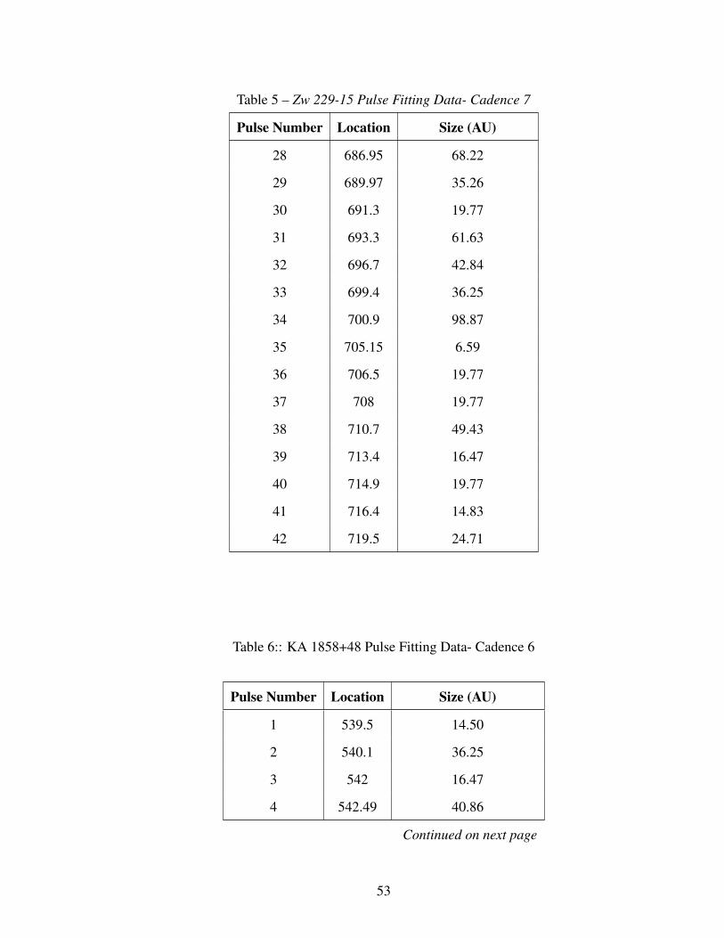
Table 5 – Zw 229-15 Pulse Fitting Data- Cadence 7
Pulse Number Location Size (AU)
28 686.95 68.22
29 689.97 35.26
30 691.3 19.77
31 693.3 61.63
32 696.7 42.84
33 699.4 36.25
34 700.9 98.87
35 705.15 6.59
36 706.5 19.77
37 708 19.77
38 710.7 49.43
39 713.4 16.47
40 714.9 19.77
41 716.4 14.83
42 719.5 24.71
Table 6:: KA 1858+48 Pulse Fitting Data- Cadence 6
Pulse Number Location Size (AU)
1 539.5 14.50
2 540.1 36.25
3 542 16.47
4 542.49 40.86
Continued on next page
53

Table 6 – KA 1858+48 Pulse Fitting Data- Cadence 6
Pulse Number Location Size (AU)
5 544.215 32.95
6 546. 47.58
7 547 59.32
8 550.15 39.54
9 551.5 19.77
10 552.6 23.07
11 553.9 13.18
12 554.2 42.84
13 556.7 131.83
14 561.6 42.84
15 564.6 59.32
16 565.4 49.43
17 567.2 39.54
18 567.9 32.95
19 568.98 16.47
20 570.2 22.74
21 571.71 21.42
22 573.06 19.77
23 574.1 12.19
24 575 32.95
25 576.75 21.42
26 578.25 24.71
27 579.2 13.18
28 580.4 26.36
Continued on next page
54

Table 6 – KA 1858+48 Pulse Fitting Data- Cadence 6
Pulse Number Location Size (AU)
29 582.1 23.07
30 583.2 13.18
31 584.1 19.77
32 587 115.35
33 589.9 13.18
34 592.5 46.14
35 595.9 54.38
36 598.9 42.84
37 599.15 28.01
38 601.1 36.25
39 603.4 59.32
40 612.8 79.09
41 617.5 65.91
42 619.9 32.95
43 621.1 16.47
44 624.4 65.91
45 627.1 23.07
46 629.6 39.54
Table 7:: KA 1858+48 Pulse Fitting Data- Cadence 7
Pulse Number Location Size (AU)
1 631.8 164.79
Continued on next page
55

Table 7 – KA 1858+48 Pulse Fitting Data- Cadence 7
Pulse Number Location Size (AU)
2 636.45 28.01
3 639.4 49.43
4 641.4 27.02
5 643.2 31.31
6 645.4 32.95
7 648.1 41.85
8 651.5 51.74
9 654.2 36.25
10 654.75 13.18
11 656.5 32.95
12 658.8 32.95
13 660.3 16.47
14 662.15 55.04
15 663.5 14.83
16 665.1 29.66
17 666.4 19.77
18 667.9 44.49
19 671.25 50.42
20 674.5 46.14
21 676.15 26.36
22 678.4 54.38
23 680.7 25.37
24 682.4 28.01
25 683.9 21.75
Continued on next page
56

Table 7 – KA 1858+48 Pulse Fitting Data- Cadence 7
Pulse Number Location Size (AU)
26 685 13.18
27 686.3 44.49
28 689 34.60
29 691.07 31.31
30 693.6 52.73
31 699.3 85.69
32 702.8 28.01
33 704.55 23.07
34 709.2 42.84
35 713.3 69.21
36 716.2 39.54
37 719.4 52.73
Table 8:: KA 1925+50 Pulse Fitting Data- Cadence 6
Pulse Number Location Size (AU)
1 540.7 194.45
2 546.3 44.49
3 548.1 31.31
4 549.2 29.66
5 550 18.12
6 551.15 22.41
7 552.1 26.69
Continued on next page
57

Table 8 – KA 1925+50 Pulse Fitting Data- Cadence 6
Pulse Number Location Size (AU)
8 552.96 25.37
9 554.8 32.62
10 555.3 29.66
11 556.9 27.35
12 558.68 24.88
13 560.1 19.77
14 560.58 6.59
15 560.78 6.59
16 561.2 13.18
17 562.3 36.25
18 564.7 32.95
19 566.7 29.66
20 568 13.18
21 569 6.59
22 569.7 56.02
23 572.5 32.95
24 572.7 13.18
25 573.92 18.12
26 574.8 6.59
27 576 56.02
28 578.9 36.25
29 580.9 27.02
30 582.8 28.67
31 584.3 18.12
Continued on next page
58

Table 8 – KA 1925+50 Pulse Fitting Data- Cadence 6
Pulse Number Location Size (AU)
32 585.4 13.18
33 585.8 24.71
34 587.85 65.91
35 590.3 26.36
36 591.2 19.44
37 592.45 24.71
38 593.85 56.02
39 594.5 25.70
40 595.5 9.88
41 596.7 32.95
42 599 32.95
43 601 29.66
44 602.7 26.36
45 604.45 29.66
46 606.7 39.54
47 611.8 62.62
48 615.5 44.49
49 617.2 16.47
50 619.6 41.19
51 621.4 16.47
52 623.3 33.94
53 625.4 29.66
54 627.35 29.66
55 629.3 27.35
59

Table 9:: KA 1925+50 Pulse Fitting Data- Cadence 7
Pulse Number Location Size (AU)
1 630.65 19.77
2 633 88.98
3 634.7 9.88
4 635.4 9.88
5 636.25 14.83
6 637.8 29.00
7 639.6 26.36
8 640.05 29.66
9 640.75 11.53
10 642.1 32.95
11 643.55 15.81
12 644.4 11.53
13 644.85 22.41
14 646.3 6.59
15 647.1 49.43
16 649.2 24.71
17 650.6 9.88
18 651.8 59.32
19 654.8 32.95
20 656.5 23.07
21 658.3 29.66
22 660.7 29.66
Continued on next page
60

Table 9 – KA 1925+50 Pulse Fitting Data- Cadence 7
Pulse Number Location Size (AU)
23 662.3 13.18
24 664.1 9.88
25 665.5 19.77
26 667.3 9.88
27 669.3 34.60
28 671.8 36.25
29 674.1 25.37
30 678.9 98.87
31 680.95 23.07
32 683.2 30.65
33 685.6 35.92
34 688.3 39.54
35 690.6 30.65
36 693.05 36.25
37 695.3 29.66
38 697.5 32.95
39 699.3 21.42
40 700.5 16.47
41 701.2 9.88
42 701.8 18.12
43 702.6 26.36
44 703.8 34.60
45 706.6 42.84
46 708.15 14.83
Continued on next page
61

Table 9 – KA 1925+50 Pulse Fitting Data- Cadence 7
Pulse Number Location Size (AU)
47 709 32.95
48 711.7 72.50
49 714.8 29.66
50 716.7 26.36
51 718.1 18.78
52 719.5 23.07
Table 10:: KA 1904+37 Pulse Fitting Data- Cadence 7
Pulse Number Location Size (AU)
1 630.4 82.39
2 636.6 131.83
3 643.1 39.54
4 646 49.43
5 649.1 16.47
6 652.4 46.14
7 655.5 42.84
8 658.2 29.66
9 661.6 52.73
10 665.9 62.62
11 670.5 56.02
12 675 56.02
13 677.5 29.66
Continued on next page
62

Table 10 – KA 1904+37 Pulse Fitting Data- Cadence 7
Pulse Number Location Size (AU)
14 679.6 36.25
15 684.5 98.87
16 687.5 42.84
17 690.9 60.97
18 694.8 56.02
19 697.7 39.54
20 698.2 23.07
21 701.3 82.39
22 706.1 65.91
23 711 79.09
24 715.8 65.91
25 716.2 26.36
26 719.4 49.43
63
Top Related