


Languages
Pages
Legal


Analysis of Bioswale Efficiency for Treating SurfaceRunoff
A Group Project submitted in partial satisfaction of the requirements of the degree
Master of Environmental Science and Management
Donald Bren School of Environmental Science and Management
University of California, Santa Barbara
By
William W. GrovesPhillip E. HammerKarinne L. Knutsen
Sheila M. RyanRobert A. Schlipf
Advisors:
Jeff Dozier, Ph.D.Thomas Dunne, Ph.D.
Analysis of Bioswale Efficiency for Treating Surface Runoff Page ii
Analysis of Bioswale Efficiency for Treating Surface Runoff
As authors of this group project, we are proud to archive it in the Davidson
Library so that the results of our research are available for all to read. Our
signatures on the document signify our joint responsibility in fulfilling the archiving
standards set by Graduate Division, Davidson Library, and the Bren School of
Environmental Science and Management.
William W. Groves
Phillip E. Hammer
Karinne L. Knutsen
Sheila M. Ryan
Robert A. Schlipf
This Group Project is approved by:
Jeff Dozier, Ph.D.
Thomas Dunne, Ph.D.

Analysis of Bioswale Efficiency for Treating Surface Runoff Page iii
Acknowledgements
The Bioswale Group would like to thank the following organizations for their
contributions in funding our research:
• Wynmark Company
• University of California Toxic Substances Research & Teaching Program,
Coastal Component
We also thank the following individuals for their valuable assistance:
Mark Linehan, Wynmark Co.
Kim Schizas, Wynmark Co.
J.T. Yean, Fuscoe Engineering
Cal Woolsey, Fuscoe Engineering
Tom Dunne, Bren School Professor
Jeff Dozier, Dean of the Bren School
John Melack, Bren School Professor
Trish Holden, Bren School Professor
Linda Fernandez, Visiting Professor
Darcy Aston, Santa Barbara County Water Agency

Analysis of Bioswale Efficiency for Treating Surface Runoff Page iv
Description of the Group Project
The group project is a major component of the degree requirements for Master’s
students in the Donald Bren School of Environmental Science and Management
at the University of California, Santa Barbara. The project allows a group of
students to tackle an issue involving both scientific investigation and
management considerations. This process is meant to serve as a realistic
introduction to working as an environmental professional. It provides the
opportunity to work and communicate successfully in a team and to complete a
professional project. The group structure allows for broader research and
analysis of environmental problems than an individual could achieve. The
process prepares individuals to successfully apply both technical and managerial
skills to solving the myriad of complex issues that face the environmental
community. The time frame for project completion is one year.

Analysis of Bioswale Efficiency for Treating Surface Runoff Page v
Abstract
Analysis of Bioswale Efficiency for Treatment of Surface Runoff
William W. Groves
Phillip E. Hammer
Karinne L. Knutsen
Sheila M. Ryan
Robert A. Schlipf
A bioswale is a low-gradient, open channel possessing a cover of vegetation
through which all surface runoff is directed. Our analysis focused on the use of a
bioswale to improve water quality exiting the site of a new project development in
Goleta, CA. Field samples and modeling predictions were used to evaluate the
overall performance of the bioswale and its contribution to decreasing pollutant
loading to the sensitive estuary, Devereux Slough. The U.S. EPA Storm Water
Management Model (SWMM) aided our understanding of future bioswale
functioning when vegetation is fully established, and this model was used to
analyze potential design modifications. We determined that the bioswale is a
cost-efficient method for addressing the project developer’s main concerns: flood
containment capacity, wetland mitigation, and reduction of pollutant loading off
site.

Analysis of Bioswale Efficiency for Treating Surface Runoff Page vi
Executive Summary
The Camino Real project is a commercial development located in Goleta,
California that includes a shopping center, entertainment facilities, associated
parking lots, and playing fields. Stormwater runoff from the project site
eventually reaches Devereux Slough, a nearby estuary. A bioswale was installed
to minimize the potential impacts of stormwater runoff to Devereux Slough. This
bioswale is expected to reduce the peak rate and total volume of stormwater
runoff and to reduce total suspended solids and pollutants in stormwater runoff
exiting the site.
The bioswale is a low-gradient, open channel possessing a dense cover of
vegetation through which all surface runoff is directed. The bioswale decreases
the speed of flows, acts as a stormwater detention facility, and allows suspended
solids to settle out. Aboveground plant parts filter particulates and their
associated pollutants as runoff passes slowly and evenly through the channel.
The pollutants are then incorporated into the soil where they may be immobilized
and/or decomposed by plants and microbes. The bioswale is considered a
creative means of controlling runoff, and has the potential to improve water
quality, mitigate wetland loss, provide flood containment, and improve the
aesthetics of the project site. As such, the bioswale has hydrologic, chemical,
and biological functions. Economic considerations are also an important aspect
for assessment of the bioswale and are addressed in the report.
The three main questions the Bioswale Group Project sought to answer were:
1) To what extent does the bioswale improve water quality?
2) What is the total impact of the bioswale in the Devereux Creek Watershed?
3) Given other available options, is the bioswale a cost-effective water treatment
method?

Analysis of Bioswale Efficiency for Treating Surface Runoff Page vii
To answer these questions, the bioswale group modeled the hydrology and water
quality of the bioswale, sampled and analyzed stormwater at the site, and
evaluated economic aspects of the use of a bioswale. The bioswale group
project used the Storm Water Management Model (SWMM) to simulate the
hydrologic and water quality processes of stormwater runoff for the Camino Real
Project site. Modeling output included total flow volumes, total pollutant loads,
hydrographs, and pollutographs for a wide range of storm events. These output
values allowed for the assessment of potential changes in stormwater runoff
quantity and quality resulting from the presence of the bioswale. We determined
that the bioswale is cost-effective, taking into account its threefold purpose: flood
containment capacity, wetland mitigation, and reduction of pollutant loading off
site. Conclusions and recommendations were based on interpretations of field
data and site observations, as well as on information from relevant documented
studies.

Analysis of Bioswale Efficiency for Treating Surface Runoff Page viii
Table of Contents
TABLE OF CONTENTS VIII
1.0 INTRODUCTION ................................................................................................... 1
1.1 PURPOSE AND NEED OF INVESTIGATION .................................................................4
2.0 BACKGROUND ..................................................................................................... 7
2.1 GENERAL DESCRIPTION OF CAMINO REAL PROJECT SITEAND ASSOCIATED AREAS ........................................................................................7
2.2 BIOSWALE DESCRIPTION .......................................................................................112.3 DEVEREUX SLOUGH ..............................................................................................162.4 STUDY DESCRIPTION .............................................................................................18
3.0 HYDROLOGIC AND HYDRAULIC PROCESSES .............................................. 21
3.1 CLIMATE ................................................................................................................213.2 HYDROLOGY OF THE SITE......................................................................................213.2.1 MEASUREMENTS AND CALCULATIONS OF OBSERVED FLOW .........................223.2.2 METHODOLOGY FOR CALCULATIONS OF PREDICTED FLOWS
WITHOUT THE ORIFICE PLATE..........................................................................333.2.3 RESERVOIR ROUTING ......................................................................................383.2.4 DETENTION TIMES ...........................................................................................403.3 HYDRAULIC DESIGN..............................................................................................423.4 SEDIMENT TRANSPORT..........................................................................................44
4.0 MODELING ......................................................................................................... 47
4.1 PURPOSE OF MODELING HYDROLOGIC AND CHEMICAL QUALITY PROCESSES ....474.2 SCREENING MODELS .............................................................................................484.3 DESCRIPTION OF SWMM ......................................................................................504.4 DESIGNATING SUBCATCHMENTS...........................................................................524.5 PARAMETERIZATION..............................................................................................554.6 CALIBRATION ........................................................................................................634.6.1 CALIBRATION OF STORMWATER RUNOFF QUANTITY.....................................634.6.2 CALIBRATION OF STORMWATER RUNOFF QUALITY .......................................74

Analysis of Bioswale Efficiency for Treating Surface Runoff Page ix
4.7 MODELING RESULTS..............................................................................................83
5.0 CHEMICAL PROCESSES ................................................................................... 93
5.1 POLLUTANTS IN STORMWATER RUNOFF ...............................................................935.1.1 SEDIMENT........................................................................................................945.1.2 NUTRIENTS ......................................................................................................945.1.3 METALS...........................................................................................................955.1.4 HYDROCARBONS .............................................................................................965.1.5 PESTICIDES AND HERBICIDES..........................................................................975.1.6 OXYGEN-DEMANDING SUBSTANCES ..............................................................975.1.7 BACTERIA........................................................................................................975.1.8 FLOATABLE DEBRIS ........................................................................................985.2 SAMPLING REGIME AND CHEMICAL ANALYSIS OF STORMWATER
AT THE CAMINO REAL BIOSWALE .........................................................................985.3 CHEMICAL SAMPLING RESULTS ..........................................................................1035.4 DISCUSSION OF CHEMICAL RESULTS...................................................................1055.4.1 WATER QUALITY CRITERIA ..........................................................................1075.4.2 SEDIMENT QUALITY CRITERIA......................................................................1095.5 TRANSPORT AND FATE OF CONTAMINANTS AT CAMINO REAL ..........................110
6.0 BIOLOGICAL CONSIDERATIONS ................................................................... 113
6.1 PHYTOREMEDIATION ...........................................................................................1146.1.1 PHYTOREMEDIATION MECHANISMS OF ORGANIC CONTAMINANTS.............1166.1.2 PHYTOREMEDIATION MECHANISMS OF HEAVY METALS .............................1176.1.3 PLANT SELECTION FOR THE BIOSWALE ........................................................1186.1.4 PLANT SPECIFICS...........................................................................................1196.1.5 SYNOPSIS OF RESEARCH ON THE UPTAKE ABILITY OF VARIOUS PLANTS....1206.1.6 LIMITS OF PHYTOREMEDIATION....................................................................1236.1.7 VEGETATION ESTABLISHMENT AND GROWTH..............................................124
7.0 ECONOMIC AND REGULATORY CONSIDERATIONS .................................. 127
7.1 WHY A BIOSWALE? .............................................................................................1277.1.1 COSTS ............................................................................................................1327.1.2 BENEFITS.......................................................................................................1337.2 REGULATORY FRAMEWORK FOR STORMWATER MANAGEMENT........................136
8.0 DESIGN ASSESSMENT ..................................................................................... 139
8.1 EXISTING BIOSWALE DESIGN STANDARDS .........................................................139

Analysis of Bioswale Efficiency for Treating Surface Runoff Page x
9.0 CONCLUSIONS ................................................................................................. 143
9.1 TO WHAT EXTENT DOES THE BIOSWALE IMPROVE WATER QUALITY? .................1439.2 WHAT IS THE TOTAL IMPACT OF THE BIOSWALE IN THE DEVEREUX CREEK
WATERSHED? ......................................................................................................1459.3 GIVEN OTHER AVAILABLE OPTIONS, IS THE BIOSWALE A COST-EFFECTIVE WATERTREATMENT METHOD? ....................................................................................................149
10.0 REPORT RECOMMENDATIONS ..................................................................... 151
10.1 EXPAND BIOSWALE MANAGEMENT PLAN ..........................................................15110.1.1 IDENTIFY TEAM MEMBERS ...........................................................................15210.1.2 ASSESS SOURCES OF POLLUTANTS ...............................................................15210.1.3 SOURCE REDUCTION .....................................................................................15210.1.4 INSPECTION ...................................................................................................15310.1.5 MAINTENANCE ..............................................................................................15410.2 REVIEW PERFORMANCE OF THE BIOSWALE ........................................................15710.2.1 MINIMUM CHEMICAL ANALYSIS RECOMMENDATIONS FOR BOTH SEDIMENT AND
WATER ...............................................................................................................15810.2.2 CHEMICAL SAMPLING CONSIDERATIONS......................................................16010.3 MAINTAIN OIL AND GREASE DEVICES ................................................................16410.4 REMOVE ORIFICE PLATE .....................................................................................16510.5 MODIFY ENERGY DISSIPATOR.............................................................................165
11.0 REFERENCES ................................................................................................... 167
12.0 PERSONS AND AGENCIES CONTACTED ...................................................... 173
APPENDIX A .................................................................................................................. A-1
A-1 HYDROLOGY CALCULATIONS .................................................................................A-1A-2 FLOW INTO THE BIOSWALE THROUGH THE ORIFICE PLATE WHEN UNDER APRESSURE HEAD ......................................................................................................................A-1A-3 FLOW EXITING THE BIOSWALE ...............................................................................A-3A-4 FLOW LEAVING THE BYPASS PIPE ..........................................................................A-4A-5 FLOW LEAVING THE ENERGY DISSIPATOR .............................................................A-4

Analysis of Bioswale Efficiency for Treating Surface Runoff Page xi
APPENDIX B .................................................................................................................. B-1
APPENDIX C .................................................................................................................. C-1
C-1 INTRODUCTION TO BEST MANAGEMENT PRACTICES..........................................C-1C-1.1 POLLUTION PREVENTION PRACTICES ...........................................................C-2C-1.2 POLLUTION REDUCTION PRACTICES ...........................................................C-10C-2 FACTORS INFLUENCING THE CHOICE OF STORMWATER BEST MANAGEMENT
PRACTICES .........................................................................................................C-14
APPENDIX D .................................................................................................................. D-1

Analysis of Bioswale Efficiency for Treating Surface Runoff Page xii
List of Figures
Figure Page
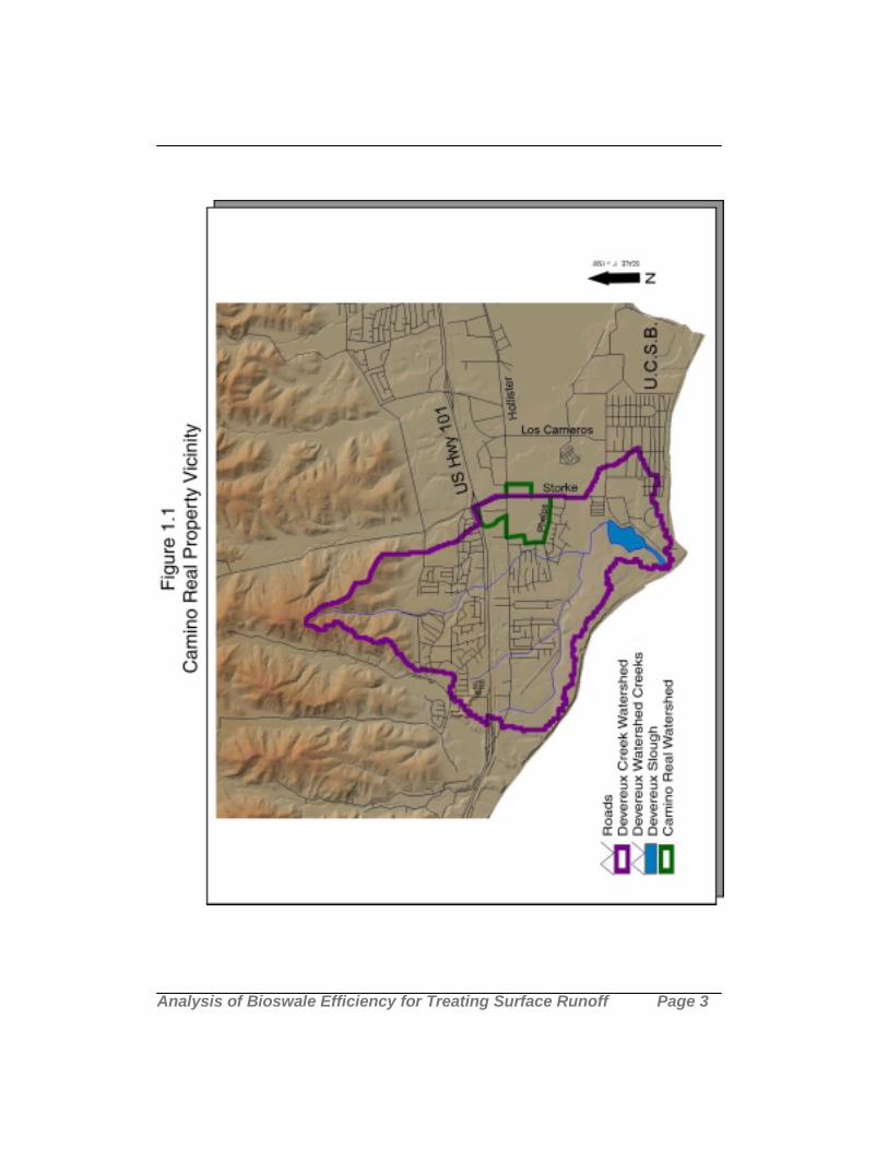
Figure 1.1 Camino Real Project Vicinity 3
Figure 2.1 Camino Real Project Site 9
Figure 2.2 Plan View of the Bioswale 12
Figure 2.3 Bioswale Backbay 15
Figure 2.4 Devereux Creek Watershed 17
Figure 3.1 Orifice Plate at the Forebay Inlet 23
Figure 3.2 Water Elevation in the Bypass Pipe Causing the Inlet
Pipe to be Under a Pressure Head 24
Figure 3.3 Energy Dissipator Discharge to the Natural Area 29
Figure 3.4 Forebay, Weir, and Berm 32
Figure 3.5 Storage-Outflow Relationship for the Bioswale 39
Figure 3.6 Hydrograph Routing through the Bioswale for a
0.15 in/hr, 2 Hour Storm 40
Figure 3.7 Detention Times of the Bioswale 41
Figure 4.1 Modeling Runoff Subcatchments 54
Figure 4.2 1/24/99 Hyetograph for Runoff at the Splitter Structure 66
Figure 4.3 1/24/99 Calibrated Hydrograph for Runoff at the
Splitter Structure 67
Figure 4.4 2/9/99 Hyetograph for Runoff at the Splitter Structure 67
Figure 4.5 2/9/99 Calibrated Hydrograph for Runoff at the
Splitter Structure 68
Figure 4.6 1/24/99 Values Observed in the Field with
Calibrated Hydrographs for the Bioswale Inlet 69

Analysis of Bioswale Efficiency for Treating Surface Runoff Page xiii
Figure 4.7 2/9/99 Values Observed in the Field with
Calibrated Hydrographs for the Bioswale Inlet 69
Figure 4.8 1/24/99 Values Observed in the Field with
Calibrated Hydrographs for the Bioswale Outlet 70
Figure 4.9 2/9/99 Values Observed in the Field with
Calibrated Hydrographs for the Bioswale Outlet 70
Figure 4.10 Calibrated Pollutograph and Observed Values for
Bioswale Inlet for the 2/9/99 Storm Event 76
Figure 4.11 Observed Values and Calibrated Pollutograph of TSS
Leaving the Bioswale Outlet for the 2/9/99 Storm Event. 79
Figure 4.12 Calibrated Pollutographs and Estimated Field Values of
Copper for the Bioswale Inlet on 2/9/99 81
Figure 4.13 Calibrated Pollutographs and Estimated Field Values of
Phosphorous for the Bioswale Inlet on 2/9/99 81
Figure 4.14 A Hydrograph and Pollutograph for TSS for the Simulation 90
Figure 5.1 Stormwater Sampling Locations 101
Figure 5.2 Erosion of Bioswale Banks 108
Figure 5.3 Transport and Fate of Pollutants at Camino Real 111
Figure 7.1 Schematic Design of a Fossil Filter® 129
Figure 7.2 Schematic Design of Stormceptor® Stormwater
Treatment Device 130
Figure 8.1 Example Bioswale from the King County Surface Water
Design Manual 142
Figure 9.1 Existing Land Use in the Devereux Creek Watershed 146
Figure 9.2 Land Use in the Devereux Creek Watershed 148

Analysis of Bioswale Efficiency for Treating Surface Runoff Page xiv
Figure C.1 Silt Fences Used During the Construction Phase of the
Camino Real Development C-4
Figure C.2 Bioswale with Mulch Applied to Slopes for Stabilization C-6

Analysis of Bioswale Efficiency for Treating Surface Runoff Page xv
List of Tables
Table Page
Table 3.1 Climatic Information for Santa Barbara, CA 21
Table 4.1 Subcatchment Parameter Values 59
Table 4.2 Subcatchment Parameter Values 60
Table 4.3 Pollutant Settling Velocity Distribution 63
Table 4.4 Comparison of Preliminary Estimates and Calibrated
Values of Parameters 68
Table 4.5 TSS Settling Velocity Distributions 78
Table 4.6 Error Between Calibrated Pollutographs and Estimate
Field Values for Copper and Phosphorous (2/9/99) 82
Table 4.7 Comparison of Bioswale Functioning With and
Without Orifice Plate 85
Table 4.8 Removal Efficiencies of the Bioswale 86
Table 4.9 Removal Efficiencies of the Bioswale and Natural Area in
Percentage of TSS Generated by the Study Site 87
Table 4.10 Removal Efficiency of the Bioswale in Percentage of TSS
Generated by the Study site 91
Table 5.1 Date, Location and Total Rainfall of Each Sampling Event 103
Table 5.2 Summary of Event Mean Concentration (EMC)
Values (mg/L) for Selected Pollutants of Samples
Collected at the K-Mart Location 104
Table 5.3 Summary of Event Mean Concentration (EMC) Values
(mg/L) for Selected Pollutants for Three Rain Events 105
Table 5.4 U.S. EPA Water Quality Criteria 106
Analysis of Bioswale Efficiency for Treating Surface Runoff Page xvi
Table 5.5 Summary of Student’s t-test of Apparent Differences in EMC
for Samples From Bioswale Inlet and Outlet 108
Table 5.6 Summary of Recommended Sediment Quality Criteria
and Forebay Sample Results 110
Table 6.1 Contaminants Suitable for Phytoremediation 118
Table 6.2 Bioswale Plant List 119
Table 7.1 Construction Costs of the Bioswale 132
Table 7.2 Comparison of Benefits Between the Bioswale and
Stormceptor® 133
Table 8.1 Dimensions of the Bioswale at Camino Real and
King County Recommendations 140
Table 10.1 Management Issues and Actions 154
Table 10.2 Recommended Parameters for Assessing the
Effectiveness of BMPs 159
Table A.1 Flow From the Site and Flows into the Bioswale and
Bypass Pipe With the Orifice Plate A-6
Table A.2 Flows Exiting the Energy Dissipator A-7
Table A.3 Storage-Outflow Relationship for the Bioswale A-8
Table A.4 Hydrograph Routing Through the Bioswale A-8
Table A.5 Flow From the Site into Bioswale and Bypass Pipe
Without the Orifice Plate A-9
Table A.6 Depth-Volume-Outflow Relationships for Bioswale Forebay,
Bioswale Backbay, and Natural Area A-10

Analysis of Bioswale Efficiency for Treating Surface Runoff Page xvii
Table D.1 Water Sampling Data from 11/7/98 Sampling Event at
K-Mart D-1
Table D.2 Soil Sampling Results for Composite Forebay Soil
Collected on 1/19/99 D-2
Table D.3 Water Sampling Data from 1/24/99 Sampling Event at
Camino Real Bioswale and Natural Area D-3
Table D.4 Water Sampling Data from 1/31/99 Sampling Event at
Camino Real Bioswale D-4
Table D.5 Water Sampling Data from 2/9/99 Sampling Event at
Camino Real Bioswale and Natural Area D-5

Analysis of Bioswale Efficiency for Treating Surface Runoff Page xviii
List of Acronyms
ACOE Army Corps Of Engineers
BMP Best Management Practice
CSO Combined Sewer Overflow
CWA Clean Water Act
EIR Environmental Impact Report
EMC Event Mean Concentration
EOA Eisenberg, Olivieri & Associates, Inc.
EPA Environmental Protection Agency
NPDES National Pollutant Discharge Elimination System
NURP Nationwide Urban Runoff Program
PAH Polycyclic Aromatic Hydrocarbon
SLAMM Source Loading and Management Model
SWMM Storm Water Management Model
TPH Total Petroleum Hydrocarbons
TSS Total Suspended Solids

Analysis of Bioswale Efficiency for Treating Surface Runoff Page 1
1.0 Introduction
The Camino Real project is a commercial development located in Goleta,
California that includes a shopping center, entertainment facilities, associated
parking lots, and playing fields. Stormwater runoff from the project site
eventually reaches Devereux Slough, a nearby estuary. (Figure 1.1). To
minimize the potential impacts of stormwater runoff on Devereux Slough, the
project’s developer, Wynmark Company, decided to install a bioswale. This
bioswale, designed by Fuscoe Engineering, is expected to reduce the peak rate
and total volume of stormwater runoff and to reduce total suspended solids and
pollutants in stormwater runoff exiting the site.
The bioswale is a low-gradient, open channel possessing a dense cover of
vegetation through which runoff is directed during storm events. The bioswale
decreases the speed of flows, acts as a stormwater detention facility, and allows
suspended solids to settle out. Aboveground plant parts filter particulates and
their associated pollutants as runoff passes slowly and evenly through the
channel. The pollutants are then incorporated into the soil where they may be
immobilized and/or decomposed by plants and microbes. The bioswale is
considered a creative means of controlling runoff, and has the potential to
improve water quality, mitigate wetland loss, provide flood containment, and
improve the aesthetics of the project site. As such, the bioswale has hydrologic,
chemical, and biological functions. Economic considerations are also an
important aspect for assessment of the bioswale and are addressed later in this
report.
The Bioswale Group Project is divided into four main components to reflect these
functions: hydrology, chemistry, biology and economic considerations. Each
component had a separate scope of work with 2 or 3 people specifically in

Analysis of Bioswale Efficiency for Treating Surface Runoff Page 2
charge of that aspect of the group project. This ensured that each area of study
received sufficient coverage, with everyone equally involved. Overlap between
the separate components allowed all group members to participate and to have
an understanding of each aspect.
Analysis of Bioswale Efficiency for Treating Surface Runoff Page 3

Analysis of Bioswale Efficiency for Treating Surface Runoff Page 4
1.1 Purpose and Need of Investigation
The three main questions the Bioswale Group Project sought to answer were:
1) To what extent does the bioswale improve water quality?
2) What is the total impact of the bioswale in the Devereux Creek Watershed?
3) Given other available options, is the bioswale a cost-effective water treatment
method?
The main focus of the group project was to analyze the functioning and
effectiveness of the bioswale. We wanted to know what impact the bioswale has
not only on the development site itself, but also in relation to the whole watershed
and its implications for Devereux Slough. It is important to note that the
completion of the group project did not coincide with the completion of all building
construction and paving at the Camino Real Development, therefore several
project findings are preliminary.
The Camino Real development is one of many changes in land use within the
Devereux Creek Watershed that have impacted the sensitive wetland and
estuarine habitat of the Devereux Slough (Davis, et al., 1990). Water flows from
the 2732 acre watershed to the 42 acres Devereux Slough Estuary. Stormwater
runoff from the watershed carries sediment and contaminants from the
watershed to the Slough. Historical land use changes have increased sediment
supply to the Slough, resulting in a reduction in the total size of the Slough and
the quality of its wetland habitats (Davis, et al., 1990). From 1965 to 1985, the
University Exchange Property immediately north of the Slough was the most
significant source of increased sedimentation. Erosion from this property has
created a fan-delta with a volume of 486,000 ft3 which occupies 13.3% of the
surface area of the Slough and has displaced 6.5% of its total volume (Davis, et

Analysis of Bioswale Efficiency for Treating Surface Runoff Page 5
al., 1990). This study also found that dissolved oxygen demand from the
watershed was negatively impacting the water quality in Devereux Slough.
Continuing urbanization of the Devereux Creek Watershed threatens to
exacerbate water quality problems for the Devereux Slough. Although 61% of
the watershed has already been urbanized by residential, commercial, and
industrial development (de la Garza and Ryan, 1998), development of the
watershed, including the Camino Real shopping center, continues to change the
quality and quantity of stormwater runoff to the Slough.
Goleta will continue to develop and grow along with the entire Santa Barbara
area. In coastal regions it is important that each new change in land use be
evaluated for potential impacts to the ecosystem. It is well documented that
developments greatly decrease pervious ground cover and increase runoff rates.
This runoff is initially characterized by an increased suspension of particles and
pollutant loads, which are detrimental to downstream areas. However, once
construction is completed, sediment loads are expected to decrease and the
system tends to stabilize. A bioswale is one solution to this problem, and this
report provides useful information for planners and developers to decide if a
bioswale is feasible given their own specific site limitations.

Analysis of Bioswale Efficiency for Treating Surface Runoff Page 6
This page intentionally left blank

Analysis of Bioswale Efficiency for Treating Surface Runoff Page 7
2.0 Background
2.1 General Description of Camino Real Project Site andAssociated Areas
The following discussion is based on information provided in the 1997 Camino
Real Project Environmental Impact Report (EIR).
The Camino Real project is an 83-acre development with a variety of land uses.
It is located at the southwest corner of Storke Road and Hollister Avenue in
Goleta, CA. Major components of the development include up to 500,000 square
feet of retail stores and other entertainment and commercial facilities. The
development contains approximately 25 acres of recreation areas and open
space, and parking spaces for approximately 3,300 cars (Figure 2.1).
The Marketplace is composed of 500,000 square feet of retail space and is
located on the northern half of the project site. 14.5 percent of the approximately
46-acre Marketplace is landscaped, with the rest of the area devoted to building
space and parking. The southern half of the project site is primarily comprised of
playing fields, open space, the bioswale, and the natural area. This combined
area is approximately 37-acres and is mostly pervious, with impervious paved
areas for approximately 400 parking spaces.
The topography of the project site slopes gently towards the south at gradients
ranging from one to two percent. The development site is part of a larger
drainage area that consists of 159 acres that is bounded on the north by U.S.
101 and includes the K-Mart Shopping Center (east of the project site) and the

Analysis of Bioswale Efficiency for Treating Surface Runoff Page 8
Santa Barbara Business Park (also east of the project site). All runoff from this
larger drainage area is directed to the bioswale and/or natural area.
A 36.3 acre section of this larger drainage area, bounded by U.S. 101 on the
north and Hollister Road on the south, consists primarily of non-native grasses.
Within this area is a housing development currently under construction and a
service station which are not a part of the Camino Real Development. The
topography of this area slopes gently towards the southeast at an overall
gradient of 1.5 percent. Approximately 33 percent of this area is impervious.

Analysis of Bioswale Efficiency for Treating Surface Runoff Page 9

Analysis of Bioswale Efficiency for Treating Surface Runoff Page 10
The 26.7 acre area comprised of the K-Mart Shopping Center and the Santa
Barbara Business Park to the east of the project also drains to the project site.
The K-Mart Shopping Center consists of commercial buildings and parking
space, with limited landscaping. The topography of this area slopes gently to the
south at a slope of 0.7 percent. Approximately 95 percent of this area is
impervious. The Santa Barbara Business Park is also located across Storke
Road to the east of the project site. It is comprised of office buildings, parking
space, and landscaping. This area slopes gently to the north at a slope of 0.8
percent and is approximately 83 percent impervious.
The existing drainage ditch on the west side of Storke Road has been replaced
with a closed storm drain pipe system. Existing storm drains from the east side
of Storke Road servicing the K-Mart Shopping Center and the Santa Barbara
Business Park have been connected to this new system. The area to the north
of the project site bounded by U.S. 101 and Hollister Road is also connected to
this system. The storm drain turns westerly at the newly constructed Santa
Felicia Drive and southerly through the parking lot before it drains into the
bioswale splitter unit. From the splitter, stormwater is either routed to the
bioswale or around the bioswale to an existing low-lying wetland depression (the
"natural area"), depending upon flow volumes. Under low-flow conditions, all
stormwater runoff is routed to the bioswale, which eventually drains to the natural
area, while under larger flow conditions, a percentage of flows bypasses the
bioswale and is routed directly to the natural area (see Figure 2.2). An additional
small pipe drains an approximately 0.5 acre playing field area adjacent to the
bioswale into the bioswale forebay. Flows from this pipe are relatively
insignificant, reaching approximately 1 cfs during the 25 year storm event. The
drainage outlet for the natural area consists of two 4.5-foot storm drains at
Phelps Road that ultimately discharge into Devereux Slough. The bioswale,
along with the natural area and adjacent playing fields, have the capacity for
storage of a 100-year storm.

Analysis of Bioswale Efficiency for Treating Surface Runoff Page 11
2.2 Bioswale Description
The project has resulted in changes to drainage patterns and an increase in
impervious surfaces, particularly on the northern portion of the site, due to the
construction of parking lots, roads, walkways, and structures. Increases in runoff
will occur due to the increase in

Analysis of Bioswale Efficiency for Treating Surface Runoff Page 12

Analysis of Bioswale Efficiency for Treating Surface Runoff Page 13
impervious surfaces and the increase in irrigation of landscaped surfaces and
turf. Increased runoff from the project could result in decreased water quality in
Devereux Slough due to the washing of pollutants from paved surfaces and
landscaped areas.
To address these concerns, the project has incorporated a bioswale to aid in the
control of stormwater runoff and its associated pollutants. The bioswale was
designed to perform three major functions:
Improve the Quality of Stormwater Runoff – The bioswale was constructed to
physically filter contaminants and facilitate the chemical and biological processes
that remove pollutants from stormwater runoff. The most important processes by
which the bioswale is expected to remove pollutants are sedimentation, filtration,
absorption, and vegetative uptake. Of these processes, sedimentation is
anticipated to be the most effective means for removing particulates and their
associated pollutants (Cunningham, et al., 1997).
Stormwater Detention – The bioswale was designed to provide stormwater
detention, which results in several benefits. The detention of stormwater reduces
peak flows from the site, thereby mitigating possible downstream flood hazards.
Decreased flow rates due to detention also promote the sedimentation of
particulates and their associated pollutants. Furthermore, lower flow rates
reduce and elongate the pollutant loading to downstream receiving waters
(Cunningham, et al., 1997).
On-site Replacement of Riparian Habitat – The bioswale is designed to
replace riparian habitat through onsite wetland mitigation. It will frequently have
saturated soil conditions, even during periods of no rainfall, because of irrigation
of the landscaping and washing of pavement. The plants chosen to go into the
bioswale are riparian and wetland native California species. The selected plants

Analysis of Bioswale Efficiency for Treating Surface Runoff Page 14
also are expected to perform wetland functions, such as taking up nutrients,
heavy metals, and organic contaminants that have settled into the soil of the
bioswale (Cunningham, et al., 1997).
The bioswale (Figure 2.2) is located at the southern end of the Marketplace area
and receives flows from the Marketplace, the area bounded by U.S. 101 and
Hollister Ave., the K-Mart Shopping Center, and the Santa Barbara Business
Park. The majority of the playing fields to the east and west of the bioswale drain
to the natural area. The bioswale is comprised of a two-staged filtration/retention
system. Runoff initially enters the bioswale structure at the storm drain splitter
directly to the east of the bioswale. This structure routes low flows to the
bioswale, while high flows are routed around the bioswale to the natural area.
Flows routed to the bioswale enter its forebay through an 1.5-foot diameter pipe.
The forebay is 26 feet wide, by 110 feet long and stores water to a depth of
approximately 2 feet. The primary purpose of the forebay is to provide
stormwater detention and particulate settling.
If the water depth in the forebay is below 2 feet, water is primarily conveyed to
the bioswale backbay through eleven 0.33-foot diameter pipes. These pipes
provide evenly distributed flows from the forebay to the backbay. Once the water
depth is above two feet, water from the forebay also flows over a broad, crested
weir to the backbay. The backbay is approximately 75 feet wide, by 290 feet
long, with a depth of approximately 4.5 feet (Figure 2.3)

Analysis of Bioswale Efficiency for Treating Surface Runoff Page 15
Figure 2.3Bioswale Backbay
When flow enters the backbay it moves along a series of meandering channels
which were designed to slow runoff velocity, carry runoff through riparian habitat,
and promote sedimentation, filtration, absorption, and vegetative uptake of
stormwater pollutants. This flow eventually ponds in a micropool at the far end of
the backbay, before leaving the bioswale through a 2-foot diameter pipe.
Flow leaving the bioswale enters the natural area. This area is a topographical
depression at the southern project site boundary adjacent to Phelps Road and
covers approximately 1.05 acres. It contains a stand of willow scrub and coastal
freshwater marsh that existed before development occurred (Cunningham, et al.,
1997). Due to its low gradient, detention storage capacity, and vegetative cover,

Analysis of Bioswale Efficiency for Treating Surface Runoff Page 16
the natural area is expected to act similarly to the bioswale in terms of improving
the quality of stormwater runoff from the project site.
2.3 Devereux SloughThe Camino Real development lies within the Devereux Creek watershed (Figure
2.4). This watershed covers an area of approximately 2,732 acres and stretches
northward from the mouth of Devereux Creek at sea level to the Santa Ynez
Mountains at an elevation of 525 feet (de la Garza and Ryan, 1998). Devereux
Creek empties into Devereux Slough which, including the area south of El
Colegio Road and the north and south fingers of Devereux Slough, contains 70
acres of wetland habitat. The quantity and quality of habitat within the slough are
currently threatened by: sediment loading, which reduces the capacity of the
slough to retain water; its total size; continued residential development in the
Devereux Creek Watershed, which increases contamination of runoff; and exotic
plant species, which displace native plants and alter habitats.
All runoff from the Camino Real Development exits through drainage pipes, then
passes underneath a housing area located to the south of the development, and
subsequently surfaces at Ocean Meadows Golf Course south of the housing
area. Water then flows through a vegetated channel within the golf course,
undergoing further filtration, and then drains to Devereux Slough.

Analysis of Bioswale Efficiency for Treating Surface Runoff Page 17

Analysis of Bioswale Efficiency for Treating Surface Runoff Page 18
2.4 Study Description
Our analysis is divided into four main sections: Hydrological Processes,
Chemical Processes, Biological Considerations, and Economic Considerations.
Following is a brief description of each section, and the intended goals.
This analysis focuses heavily on the hydrologic and hydraulic aspects of the
bioswale. Hydraulics and hydrology, along with site geology, are fundamental in
choosing a stormwater treatment system, as they provide the foundation for what
methods are feasible given the site conditions. This information is also required
to quantify how the bioswale functions and its overall effectiveness. Water
samples from the development site were collected from several rain events and
chemically analyzed. These data were used to calibrate the Storm Water
Management Model, which was then used to simulate possible future storms and
show how the bioswale and natural area would perform.
The chemical section describes which chemicals are regarded as potential
problems in surface runoff according to literature reviews, and then lists the
chemicals we tested in our analysis. An explanation is provided on why these
potential pollutants were chosen, followed by a description of our sampling
regime and analysis. This section pinpoints which pollutants are of most concern
given the particular site conditions.
The biological section focuses on phytoremediation, which is the use of plants to
remediate polluted water or soil, and summarizes relevant literature. The
bioswale is vegetated, mostly with wetland plant species that are expected to aid
in pollutant degradation. Included is a list of plant species in the bioswale and
known information on their role in phytoremediation. Also discussed are limits to
the establishment and growth of vegetation within the bioswale and the
classification of the bioswale as on-site wetland mitigation.

Analysis of Bioswale Efficiency for Treating Surface Runoff Page 19
The economic section evaluates the cost-effectiveness of the bioswale given
certain requirements such as wetland mitigation, minimization of pollutant-loading
offsite, and flood containment. The potential for aesthetic enhancement and
maintenance of good community relations were also a priority. We present a
summary of costs associated with bioswale construction and discuss benefits of
the bioswale versus alternative treatment options. This information provides
information for future land planning decisions.
We complete the analysis with conclusions and recommendations based on
current data. The study was conducted during the construction phase of the
project therefore several of our findings are preliminary. Ongoing research
should be conducted to fully understand and assess the performance of the
bioswale as a stormwater runoff management practice.

Analysis of Bioswale Efficiency for Treating Surface Runoff Page 20
This page intentionally left blank

Analysis of Bioswale Efficiency for Treating Surface Runoff Page 21
3.0 Hydrologic and Hydraulic Processes
3.1 ClimateSanta Barbara County has a Mediterranean climate with warm, dry summers and
cool, often wet winters. Inland, weather tends to be more seasonal.
Temperatures in the county can drop into the 20s in the northern interior during
winter nights, although coastal temperatures remain mild - with highs in the mid-
60s and lows in the 40s. Spring starts the warming trend toward summer when
average temperatures range from the low-70s along the coast to the mid-80s in
the valleys and the low-90s further inland. Precipitation falls predominantly
between November and March. Monthly temperature and precipitation data are
listed in Table 3.1.
Table 3.1Climatic Information for Santa Barbara, California
Jan Feb Mar Apr May Jun Jul Aug Sep Oct Nov Dec AnnAverageDaytimeTemp (°F)
63 65 65 68 69 71 74 75 75 73 69 65 69
AveragePrecip (in) 3.8 3.4 2.8 1.2 0.2 0.1 0.1 0.1 0.3 0.4 1.8 2.4 16.124 HourMaximumPrecip (in) 4.0 4.0 4.5 1.7 1.2 0.4 0.9 1.0 3.0 2.4 2.9 2.6 4.5
3.2 Hydrology of the Site
The Camino Real watershed, which drains the Camino Real Development and
the surrounding area, is 159 acres. The majority of the 159 acres is largely
impervious commercial and residential development with extensive parking lots.
Forty-one acres are primarily composed of playing fields, which will drain directly
to the natural area. The primary purpose of the bioswale is to mitigate pollutants

Analysis of Bioswale Efficiency for Treating Surface Runoff Page 22
associated with parking lot runoff. Stormwater is routed to the bioswale from the
surrounding area through a pipe network. Near the bioswale forebay, a flow
splitter in the piping system divides flow. A 1.5-foot diameter pipe conveys flow
to the bioswale, and a 5.5-foot diameter pipe is placed directly above this pipe to
route additional flow directly to the natural area in the case of a high flow event.
This split flow design has two functions: 1) It directs all low flow events, small
storms, irrigation, and site washdowns to the bioswale and 2) It directs the first
portion of a high flow event, large storms to the bioswale. Since the bioswale
can only treat a limited volume of stormwater runoff, this split flow design
maximizes its pollutant filtration capacity by treating highly concentrated low
flows and the first flush of larger storms. The two primary means of mitigating
stormwater runoff in the bioswale will be through the settling of particulates and
plant filtration. Both of these removal mechanisms are more efficient the longer
the water is present within the bioswale. Therefore detention times were
calculated for a number of storm events in order to determine the effectiveness of
the bioswale.
The Storm Water Management Model was used to determine the routing and
volume of runoff from the Camino Real project site, and a Fuscoe engineering
report (1997) was consulted to determine the amount of flow discharging from
the natural area. For the storm events sampled flows were measured at the inlet
and outlet of the bioswale and the outlet of the natural area (Figure 2.2). The
purpose for taking these measurements was to determine a mass loading for
problematic pollutants associated with stormwater runoff, and the effectiveness
of the bioswale and natural area in mitigating these pollutants. All of the flow
measurement results are included in Appendix D.
3.2.1 Measurements and Calculations of Observed Flow

Analysis of Bioswale Efficiency for Treating Surface Runoff Page 23
This section describes the methodology used for determining field
measurements. In evaluating the design of the bioswale it was important to get a
quantitative understanding of the conveyance of water to the bioswale, through
the bioswale, and to the natural area. Currently, a one-foot orifice plate is placed
over the 1.5-foot inlet pipe to the forebay to help aid in flow measurements
(Figure 3.1).
3.2.1.1 Flow Entering the Bioswale
To calculate the flow entering the bioswale, the height of water with respect to
the orifice plate was recorded, and a chart provided by Fuscoe Engineering was
then consulted to determine the amount of water entering the bioswale.
However, the orifice plate proved to be useful only in very low flows because
measurement markings became covered by ponded stormwater. Consequently,
the flow to the bioswale had to be calculated based on the upstream head and
the head at the exit of the inlet pipe (Figure 3.2).
Figure 3.1Orifice Plate at the Forebay Inlet

Analysis of Bioswale Efficiency for Treating Surface Runoff Page 24
Figure 3.2Water Elevation in the Bypass Pipe Causing the Inlet Pipe to be under a
Pressure Head

Analysis of Bioswale Efficiency for Treating Surface Runoff Page 25
The velocity leaving the orifice plate is assumed to be similar to that of a
submerged jet (Daugherty, et al., 1985). Therefore, the following equation was
used to calculate the velocity of water entering the bioswale.
(3-1) V0= (2*g*∆H)1/2
Where: V0 = the velocity of the discharge (ft/s)
g = gravitational acceleration ( 32.2 ft/s2)
∆H = the change in head (ft)
The height of water was measured at the entrance to the forebay and at the exit
of the bypass pipe using a dipstick. It was the intention of the bioswale group to
measure the upstream head where the bypass pipe and inlet pipe to the bioswale
meet. Unfortunately, the parking lot adjacent to the bioswale went under
construction a few days before the first rain event and the manhole where
measurements could be taken was temporarily paved over. As a result, inflow to
the bioswale had to be estimated. The height at the exit of the bypass pipe was
extrapolated back to where it would cause the inlet pipe of the bioswale to be
under a pressure head (Figure 3.2). For the January 24th and February 9th rain
events this height was assumed to be 0.33-feet (2”), higher than the height
recorded at the exit of the bypass pipe. There will be further discussion as to
why adding two inches is a valid estimate for these sampling events when the
estimation of head water for large flows from the bypass pipe is discussed. The
following equation was then used to calculate the resulting flow to the bioswale.

Analysis of Bioswale Efficiency for Treating Surface Runoff Page 26
(3-2) Q = K*A0*(2*g*∆H)1/2
Where: Q = the discharge in (ft3/s)
K = coefficient
A0 = area of the orifice plate (ft2)
g = gravitational acceleration ( 32.2 ft/s2)
∆H = the change in head (ft)
The coefficient (K) was determined from tables relating it to the Reynolds number
of approach and the orifice to pipe diameter ratio (Daugherty, et al., 1985). This
calculation is provided in Appendix A. Table A.1 in Appendix A illustrates flows
to the bioswale and bypass pipe as well as the height changes between the
bypass pipe and the inlet pipe for a number of flow events.
3.2.1.2 Flow Exiting the Bioswale, Bypass Pipe and Natural Area
In determining the amount of flow leaving the bioswale backbay, Manning’s
equation was used when the flow was not under a pressure head. In all storm
events sampled the flow leaving the backbay behaved as open channel flow.
This same theory was applied for the bypass pipe and the outlet pipes of the
natural area. The Manning equation is:

Analysis of Bioswale Efficiency for Treating Surface Runoff Page 27
(3-3) V = 1.49*R2/3*S1/2/n
Q = V*A
Where: V = velocity (ft/s)
R = hydraulic radius (ft)
S = slope of the hydraulic grade line (ft/ft)
n = Mannings roughness coefficient (s/ft-1/3)
A = area of the pipe (ft2)
Q = discharge (ft3/s)
The slope of the bioswale exit pipe, the bypass pipe, and the outlet pipes of the
natural area were determined from consulting Fuscoe Engineering’s design
plans. Manning’s roughness coefficient values were determined from consulting
a table which provided Manning’s roughness coefficient values for a wide range
of surface and channel types (Daugherty, et al., 1985). A dipstick was used to
determine the height of water leaving the bioswale exit pipe, the bypass pipe,
and the outlet pipes of the natural area. In determining the hydraulic radius and
area for flow in a partially filled pipe, a table consisting of geometric relationships
for circular pipes was consulted (Hammer, et al., 1993).
3.2.1.3 Observed Backflow from the Energy Dissipator to the Bioswale
During the sampling of storm events, we observed that the water leaving the
bypass pipe and bioswale exit pipe was accumulating in the energy dissipator.
Because the timing of sampling at the exit of the bioswale was based on
previously calculated detention times, a concern was raised that due to water
accumulating in the energy dissipator an exit loss could significantly increase the
detention time of the bioswale. There was also a concern that in the case of a
heavy rain event, runoff would accumulate so rapidly in the energy dissipator that

Analysis of Bioswale Efficiency for Treating Surface Runoff Page 28
a reverse pressure gradient could form, thereby causing water to flow back into
the bioswale. Therefore calculations had to be performed which took water
accumulation in the energy dissipator into consideration.
To calculate the flow leaving the energy dissipator it was necessary to determine
its precise dimensions. Onsite measurements revealed that the length of this
device was approximately 21 feet, with a width of 16 feet. Water leaves the
energy dissipator through three 0.5-foot openings (Figure 3.3). Once the water in
the energy dissipator reached a height of 2.75-feet it would leave through the
whole width of 16 feet. It was determined that the equation for a suppressed
rectangular weir would be most appropriate to calculate flow through the three
0.5-feet openings. If the height of water exceeded 2.75-feet, the equation for a
broad-crested weir would be used to determine the flow of this additional water.
Considering the effects of the velocity of approach will yield the following
equation for a suppressed rectangular weir (Daugherty, et al., 1985, and U.S.
Bureau of Reclamation, 1984).
(3-4) Q = 3.33*L*[(H + h)3/2 –h3/2]
Where: Q = discharge (ft3/s)
L = length of the weir (ft)
H = height of water relative to the crest (ft)
h = V2/2g (ft)
The length of the weir was measured in the field, and the height of water relative
to the crest was measured in the field while sampling, but could also be
determined theoretically based on the amount of flow entering the energy
dissipator. This is possible, since the flow is expected to reach a steady state
very quickly because the device is so small. The height of water should be
measured at a distance upstream at least four times that of the maximum head

Analysis of Bioswale Efficiency for Treating Surface Runoff Page 29
employed due to drawdown (Daugherty, et al., 1985). This was taken into
consideration in field measurements as well as theoretical calculations. Since
the velocity approaching the sharp-crested weir will be critical before it moves
over the weir, the Froude number is one (Daugherty, et al., 1985). Therefore the
velocity of approach can be calculated from the Froude number as follows:
(3-5) F = V/(g*H)1/2
Where: F = Froude number (1 for critical flow)
V = velocity of approach (ft/s)
g = gravitational acceleration ( 32.2 ft/s2)
H = the depth of the water (ft)
From these values it is possible to calculate the discharge of the energy
dissipator for any value of H as well as the amount of water that will accumulate
in it (Figure3.3).
Figure 3.3Energy Dissipator Discharge to the Natural Area

Analysis of Bioswale Efficiency for Treating Surface Runoff Page 30
Table A.2 in Appendix A indicates the height of water in the energy dissipator,
the resulting discharge to the natural area, and field observations. It was
concluded that a reverse pressure gradient would form causing the bioswale to
begin filling at the outlet even in the case of a small rain event. Currently, the
total flow from the site would only have to be about 10 ft3/s for this to occur. On
February 9, 1999 a reverse pressure gradient was observed and the bioswale
began filling at its outlet. As a result, calculations of detention times for observed
conditions in the bioswale were only made for small rain events, as it would be
difficult to incorporate this phenomenon.
3.2.1.4 Calculation of Observed Detention Times
Once discharge relationships for associated heights and volumes within the
bioswale were determined, it was possible to estimate detention times for water
in the forebay and backbay. The capacity of the forebay before the weir begins
to transfer flow to the backbay is roughly 6000 ft3. For the purpose of calculating
its detention time, it was assumed that the water entering the forebay was
leaving at the same rate unless otherwise observed. The following equation was
used to estimate the detention time of the forebay.
(3-6) td = V/Q
Where: td = the detention time of the forebay
(seconds)
V = the volume of the forebay (ft3)
Q = outflow (ft3/s)

Analysis of Bioswale Efficiency for Treating Surface Runoff Page 31
As noted above, it is very likely that the weir will be discharging water to the
backbay, thus it is likely that a steady state will be reached in the forebay.
However, if the weir was not activated, flow to the backbay would have to be
measured leaving the eleven 0.33-foot diameter pipes (Figure 3.4), and the
height of water would have to be measured in the forebay to determine its
volume at partial capacity. With these measurements the above equation could
still be employed to determine the detention time of the forebay.
The detention time of the backbay is estimated by measuring the height of water
at the outlet pipe. For this height, the volume of water present in the backbay
can be determined as well as the rate at which it is discharging. The volume of
water that has ponded was determined from consulting the Fuscoe Engineering
plans (1997) for variations of elevation in the backbay. The ponding elevations
derived from the Fuscoe Engineering plans matched well with visual
observations while sampling. The water present in channels flowing to the
ponded area was also considered in calculating the detention time. The speed at
which this water reached the ponded area was determined to be irrelevant, since
the time for the ponded area to discharge was much greater than the time of
travel through the backbay. In calculating the detention time of the backbay
equation 3-6 can be used.
Analysis of Bioswale Efficiency for Treating Surface Runoff Page 32
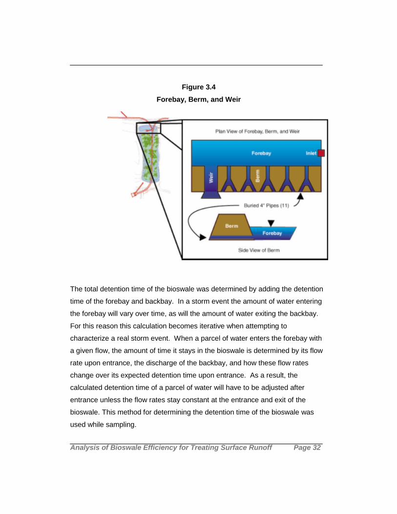
Figure 3.4Forebay, Berm, and Weir
The total detention time of the bioswale was determined by adding the detention
time of the forebay and backbay. In a storm event the amount of water entering
the forebay will vary over time, as will the amount of water exiting the backbay.
For this reason this calculation becomes iterative when attempting to
characterize a real storm event. When a parcel of water enters the forebay with
a given flow, the amount of time it stays in the bioswale is determined by its flow
rate upon entrance, the discharge of the backbay, and how these flow rates
change over its expected detention time upon entrance. As a result, the
calculated detention time of a parcel of water will have to be adjusted after
entrance unless the flow rates stay constant at the entrance and exit of the
bioswale. This method for determining the detention time of the bioswale was
used while sampling.

Analysis of Bioswale Efficiency for Treating Surface Runoff Page 33
In calculating the flow leaving the natural area a dipstick was used at the outlet
pipes to determine the height of water at exit in this detention basin. The height
measurements at the outlet area of the natural area were approximate as the
pipe was not readily accessible and the dipstick had to be read from a distance of
about ten feet. Manning’s equation was used to calculate the resulting
discharge.
3.2.2 Methodology for Calculations of Predicted Flows without theorifice plate
3.2.2.1 Removal of the Orifice Plate
The purpose of this section is to provide flow calculations for the bioswale for
how it is expected to perform in the future. In studying the bioswale, it has
become apparent that the orifice plate will have to be removed for optimal
bioswale performance. Although the orifice plate is a useful tool in flow
measurement, it is a flow impediment. The orifice plate is causing a significant
amount of flow to be routed around the bioswale that would otherwise have been
treated. Since the main purpose of the bioswale is to catch the first flush of
pollutants associated with stormwater runoff, the orifice plate is detrimental to the
effectiveness of the bioswale. Consequently, we have recommended the
removal of the orifice plate and calculated flows without the orifice plate.
However, without the orifice plate, different methods have to be employed for
determining the hydrological processes within the bioswale.
The effect of removing the orifice plate on the conveyance of flow to the bioswale
was significant. As stated earlier, it was not possible to calculate large flow
events for the bioswale with the orifice plate as the energy dissipator would
accumulate too much water, thereby causing the bioswale to receive water at

Analysis of Bioswale Efficiency for Treating Surface Runoff Page 34
both its inlet and outlet. Without the orifice plate it was possible to calculate flows
up to the twenty-five year storm.
3.2.2.2 Flow at the Bioswale Inlet
The bioswale inlet pipe will behave as open channel flow until it becomes ponded
to an elevation above the height of the 1.5-foot diameter pipe. Since the forebay
fills up quickly, the flow to the bioswale will frequently be under a pressure head
(Figure 3.2). To calculate this flow the energy equation was employed.
(3-7) ρ1/λ1 + V12/2g + z1 = ρ2/λ2 + V2
2/2g + z2 + hL
Where: ρ/λ = pressure head (ft)
V2/2g = velocity head (ft)
z = elevation head (ft)
hL = head loss (ft)
ρ = pressure (lb/ft2)
λ = specific weight (lb/ft3)
v = velocity (ft/s)
g = gravitational acceleration (ft/s2)
When flow to the bioswale is under a pressure head several terms in this
equation are negligible. The pressure heads at both the inlet of the forebay and
the splitter are zero since they are measured at the water surface (Figure 3.2).
The velocity head at the inlet to the forebay is zero since it is measured at the
water surface of this reservoir. The velocity head at the splitter is zero since the
flow to the bioswale is perpendicular to flow coming into the splitter, it is flowing
in the y direction and the concern is the amount of flow to the bioswale which is
in the x direction. Thus, for this application equation 3-7 can be rewritten as
follows:

Analysis of Bioswale Efficiency for Treating Surface Runoff Page 35
(3-7) ∆Z = hL = f*L*V2/D*2g
Where: ∆Z = the change in elevation between points
one and two (ft)
f = the friction factor (dimensionless)
L = the length of the pipe (ft)
V = the velocity (ft/s)
D = the diameter of the pipe (ft)
g = gravitational acceleration (32.2 ft/s2)
The change in elevation the upstream head was estimated from consulting a
culvert capacity chart for a circular concrete pipe with a diameter of 5.5-feet (U.S.
Bureau of Public Roads, March 1965). The length of the bypass pipe is 420 feet,
however, the 5.5-foot diameter bypass pipe has a broken slope. For the first 23
feet the slope is 0.146 and for the last 397 feet it is 0.002. Since all the other
requirements for the use of the culvert capacity chart were met, the chart can still
be used even if a broken slope is present within the pipe (U.S. Bureau of Public
Roads, March and December 1965). Following the procedure outlined for the
use of the culvert capacity charts with a broken slope, it became apparent that
the effect of the broken slope present on the upstream headwater for a given flow
exiting the bypass pipe is negligible. Manning’s equation with a slope of 0.002
was used to calculate the flow leaving the bypass pipe, and a culvert capacity
chart was consulted to obtain the height of the water upstream (Figure 3.2).
Thus, for a given amount of flow bypassed around the bioswale the upstream
head can be calculated. The results of this analysis and are presented in
Appendix A in Table A.1. The culvert chart does not provide upstream head
estimates for low flows. However, for low flow events, the height change
estimate given by the culvert chart between the exit of the bypass pipe and its
upstream water surface would be between zero and 0.33-feet (4-inches). Since

Analysis of Bioswale Efficiency for Treating Surface Runoff Page 36
it is not known if the subsequent decrease in height change is linear, a value of
0.17-feet (2-inches) was estimated for flows that the culvert capacity chart does
not provide. The amount this would change the flow to the bioswale is not
significant.
For the bioswale inlet head a flow to the bioswale was estimated for the change
in elevation between the head at the inlet and the upstream head at the splitter
(Figure 3.2). Since the forebay is expected to reach a steady state under such
conditions, a trial and error process could be employed to determine the flow to
the bioswale for a given upstream head. The application of Moody’s diagram
shows that the Reynolds number was significant enough to cause a constant
friction factor for the flows in question.
3.2.2.3 Flows From the Forebay to the Backbay
In determining the amount of flow from the forebay to the backbay, the equation
for a broad crested weir was used (Daugherty, et al., 1985).
(3-8) Q = L*g1/2*(2/3)3/2*H3/2
Where: Q = flow in ft3/s
L = length of the weir (ft)
g = gravitational acceleration (32.2 ft/s2)
H = height of flow over the weir (ft)
The elevation throughout the forebay was assumed to be constant. This
assumption matched well with observed conditions. During one storm event the
elevation at the bioswale inlet was measured at 19 feet above mean sea level,

Analysis of Bioswale Efficiency for Treating Surface Runoff Page 37
while an elevation of 19.15 feet would be expected from calculations. This
discrepancy is small and may be due to the weir not being constructed exactly as
the site plans indicated or possibly an error in field measurements.
Determination of the flow from the forebay to the backbay through the eleven
0.33-foot pipes was difficult since the pipes branch out into twenty-two pipes
before exiting into the backbay. These pipes will initially be under a pressure
head and then once they branch out, will start behaving as open channel flow.
The pipes should each convey a similar amount of flow to the backbay.
However, during sampling events it was evident that flow exiting these pipes was
inconsistent. Some pipes were approximately half full, while others were
conveying a trickle of water. Therefore, the amount of discharge through these
pipes had to be estimated based on field observations. The discrepancy in flow
through these pipes may have been due to clogging from sediment.
3.2.2.4 Flow from the Backbay to the Natural Area
In estimating the amount of flow leaving the backbay, Manning’s equation was
used if the flow was behaving as open channel flow. However, for rain events up
to the 25-year storm, this pipe will be under a pressure head. The energy
equation was used in calculating this flow. The pressure head at the exit of the
backbay and the entrance to the energy dissipator will be zero since they are
measured at the water surface. The velocity head at the exit of the backbay
should be zero since it is measured at the water surface of this reservoir. In the
energy dissipator the velocity head is assumed to be negligible because it is
measured at the water surface directly above the 2-foot exit pipe of the backbay.
In estimating the change in height between the bioswale exit and the energy
dissipator, a trial and error process was once again necessary. In calculating the
detention time for design rain events, a discharge through the bypass pipe was

Analysis of Bioswale Efficiency for Treating Surface Runoff Page 38
assumed. From this discharge the upstream headwater and the subsequent flow
to the bioswale can be calculated as outlined above.
3.2.2.5 Backflow to the Bioswale in Large Flows
Since the flow out of the bypass pipe and the flow leaving the bioswale is known,
the energy dissipator chart can be consulted to determine the height of water in
this device to achieve the outflow desired. If the height of water in the energy
dissipator is known, the height of water necessary for the correct conveyance of
flow from the bioswale can be calculated through a trial and error process. With
the orifice plate removed the possibility of a reverse pressure gradient in the
energy dissipator is unlikely since the amount of flow into the bioswale is
significantly increased. Due to the iterative nature of this calculation, it cannot be
completely ruled out, but if a reversal of flow was to occur it would most likely be
in a heavier storm after the problematic first flush had already been captured by
the bioswale. Even if a reverse pressure gradient were to occur, it would be
overcome in a few minutes as flow builds up in the bioswale.
3.2.3 Reservoir Routing
The purpose of performing reservoir routing on the bioswale for a design storm is
to determine if the Storm Water Management Model (SWMM), discussed in
Section 4 is properly routing stormwater through the bioswale. The discussion of
reservoir routing follows Dunne and Leopold’s reservoir routing method (1978).
To apply reservoir routing to the bioswale it was necessary to first determine its
storage-outflow relationship. The height of water in the bioswale and its
associated volume and discharge have been derived earlier in this report.
Calculations for storage-outflow relationships are included in Appendix A, Table
A.3. In this example the chosen time increment was 15 minutes. Figure 3.5
illustrates the storage-outflow relationship for the bioswale.

Analysis of Bioswale Efficiency for Treating Surface Runoff Page 39
Once the storage-outflow relationship has been derived it is possible to route
stormwater through the bioswale. The Storm Water Management Model was
used to produce an inlet hydrograph. A 0.15 in/hr, two-hour storm was the
design storm used in this example. The values for hydrograph routing through
the bioswale are presented in Table A.4 in Appendix A. From the inlet
hydrograph it was possible to determine the inflow into the bioswale for 15-
minute time steps. The average inflow rate is calculated for each 15-minute time
step. At the beginning of an interval the outflow is taken from the previous
interval to determine (S1/∆t – O1/2) in column 4 in Table A.4, by consulting Figure
3.5. In column 5, (S2/∆t + O2/2) is determined by adding the average inflow for
this interval to (S1/∆t – O1/2). Figure 3.5 can be consulted again to determine the
outflow rate at the end of the time interval. This process is repeated as illustrated
in Table A.4 in Appendix A.
Figure 3.5 Storage-Outflow Relationship for the Bioswale
0.005.00
10.0015.0020.0025.0030.0035.0040.00
0.08
0.78
2.21 3.9 5 5.9 14
.9
Rate of Outflow (cfs)
Stor
age-
Out
flow
fu
nctio
ns (c
fs)
s(t)-o/2s(t)+o/2

Analysis of Bioswale Efficiency for Treating Surface Runoff Page 40
The expected outlet hydrograph of the bioswale from the Storm Water
Management Model closely matches with the outlet hydrograph obtained from
reservoir routing (Figure 3.6). Therefore, according to reservoir routing the Storm
Water Management Model appears to be producing a fairly accurate outlet
hydrograph for the bioswale.
3.2.4 Detention times
In calculating the detention times, the bioswale is assumed to be at a steady
state, so the flow that is going to the bioswale should be leaving the bioswale at
the same rate. With a hydrograph, reservoir routing can be used to determine
the amount of outflow and its timing for a given amount of inflow. The
determined outflow can then be used to calculate the detention time for a parcel
of water. The steady-state assumption does not consider that outflow will be
changing over time for a parcel of water as reservoir routing does. But, for the
purpose of illustrating how the bioswale will perform for a number of outflows the
steady-state assumption was used. Figure 3.7 plots expected detention times of
Figure 3.6 Hydrograph Routing through the Bioswale for a 0.15 in/hr 2 hour storm
0.0
2.0
4.0
6.0
8.0
10.0
0 30 60 90 120
150
180
210
Time (minutes)
Rat
e of
Out
flow
(cfs
)
Rate of Inflow(SWMM)Reservoir RoutingOutflowSWMM outflow

Analysis of Bioswale Efficiency for Treating Surface Runoff Page 41
the bioswale without the orifice plate using a steady-state assumption. In
applying this plot to a storm event, outflows would have to be recorded
throughout the storm and then averaged for the expected time a parcel of water
stays within the bioswale. The Storm Water Management Model, which is further
discussed in Section 4, could also be used as it produces a similar outlet
hydrogaph to the one obtained from reservoir routing.
Figure 3.7Detention Times of the Bioswale
The detention time will decrease for inflows up to about 15 ft3/s, and then begin
to slowly increase for inflows up to 40 ft3/s (Figure 3.7). While intuitively the
detention time of the bioswale would be expected to decrease as the inflow
increases, the design of the bioswale causes an increasing detention time with
increasing inflow. As with most detention basins, the residence time will be high
in low flow events, but as the volume of the detention basin increases due to
inflow, the drop off in detention time becomes less dramatic (Figure 3.7).
However, in the case of the bioswale at Camino Real, once the inflow begins
increasing above 15 ft3/s, there is a significant increase in the amount of flow that
is routed through the bypass pipe, thus increasing the height of water in the

Analysis of Bioswale Efficiency for Treating Surface Runoff Page 42
energy dissipator. Since the flow exiting the bioswale will be under a pressure
head, the elevation in the bioswale will have to increase more than expected to
make up for the increased height in the energy dissipator. The kink in Figure 3.7
around an inflow of 15 ft3/s is when the effect of the energy dissipator becomes
noticeable. The energy dissipator causes the flow to level out from an inflow of
about 20 ft3/s to an inflow of about 35 ft3/s. From an inflow of 35 ft3/s to an inflow
of 40 ft3/s, the detention time begins to increase at a linear rate. The second kink
in the curve is due to a changing control mechanism for the height of water in the
forebay. Up to this point, flow was being transferred from the forebay to the
backbay over a broad crested weir. With an inflow of greater than 35 ft3/s the
backbay will pond to the same elevation of the forebay. Therefore, the elevation
of water in the bioswale became constant throughout. The detention time of the
forebay began to increase from this time step forward as discharge of water to
the backbay had become less efficient. Consequently, the result is a slight
increase in detention time when inflows increase from 35 to 40 ft3/s.
3.3 Hydraulic Design
The purpose of the following section is to discuss the hydraulic design of this
bioswale, and possible improvements that could have been made given the
limited space available. In studying the hydraulic design of the conveyance of
water through the bioswale and around it, we emphasize the following areas for
discussion: hydraulic design, the slope of the bypass pipe, and the use of an
energy dissipator. The overall sizing of the bioswale will not be discussed in this
section, as there was a limited amount of space available for its design.
The use of a forebay and backbay in the design of the bioswale is recommended
in a number of studies, and is instrumental in increasing the detention time of the
bioswale (Wanielista, et al., 1986). The use of a bypass pipe is recommended

Analysis of Bioswale Efficiency for Treating Surface Runoff Page 43
and since the purpose of a detention basin is to catch the first flush of pollutants,
if a bypass pipe is not present the detention basin would be overrun with water,
therefore causing it to be less effective. The fundamentals of an effective
detention basin design for the treatment of urban stormwater runoff are present
in the design of this bioswale. However, there are a few areas in the design of
this bioswale, which are not optimal for bioswale performance.
If the capacity of the forebay were increased, this could significantly increase the
detention time of the bioswale for smaller rain events, thereby causing it to be
more effective in its ability to remove pollutants. See the modeling results
(Section 4.7) for further discussion of this subject.
Another area of concern is the slope of the bypass pipe and the use of an energy
dissipator. As noted above a break in the slope exists in this 5.5-foot pipe. Flow
leaves this pipe with a slope of 0.002, yet the average slope for the whole pipe is
0.01. The optimum slope of a culvert of this size can be calculated by the
following formula (Simon, 1986).
(3-9) Soptimum = 111*n2/D1/3
Where: n = Manning’s roughness coefficient (s/ft-1/3)
D = diameter of the pipe (ft)
S = the slope of the pipe (ft/ft)
It should be noted that these units do not cancel out, so it is assumed that the
coefficient will remedy this discrepancy. For the 5.5-foot concrete culvert the
optimum slope for the conveyance of water is 0.01. But, as noted above the
water is discharged to the energy dissipator with a slope of only 0.002.
Therefore, the culvert is not discharging the optimum amount of water due to its
smaller gradient and resultant slower velocity.

Analysis of Bioswale Efficiency for Treating Surface Runoff Page 44
The impetus behind putting an energy dissipator at the discharge points of
culverts is to slow down the velocity to prevent erosion. However, this energy
dissipator is designed so that it accumulates water, because flow is allowed to
only discharge through a very small area. As flow is ultimately discharged
through these three 0.5-foot openings, the energy dissipator actually increases
the velocity, thereby defeating its ability to mitigate erosion processes (Figure
3.3). However, the same characteristics of the energy dissipator that cause it to
increase the velocity, also cause it to accumulate water. This has the effect of
increasing the detention time of water within the bioswale for reasons outlined
earlier in Section 3.2.2.
3.4 Sediment Transport
As sediment accumulates in the bioswale there is the possibility that it could be
scoured up in a heavy rain event, causing pollutants originally removed by the
bioswale to be loaded to the natural area and possibly to Devereux Slough. In
determining if such an event will occur it is necessary to obtain the distribution of
sediment sizes that have been deposited, where it accumulates, as well as the
velocity that would cause particles of a certain size to become mobile. Since the
possibility of sediment transport is most likely in the case of a heavy rain event,
the bioswale would be functioning as one channel as it would be entirely
submerged in water. Therefore, it is possible to calculate the velocity of water
through the bioswale by applying Manning’s equation using a width of 75 feet, a
slope of 0.0045 and the depth that would convey the flow in question. To
determine where and how particles will accumulate in the bioswale further field
work would be necessary, although it is likely that most sediment particles will
accumulate in the forebay or the back of the backbay as this is where stormwater
ponds within the bioswale. Since most pollutants are trapped in fine grain
sediments, the transport of this type of sediment is of most concern. The

Analysis of Bioswale Efficiency for Treating Surface Runoff Page 45
deposition rates of sediment and fine-grained particles could be estimated based
on the removal efficiency of the bioswale for the rain events sampled. However,
the bioswale is currently under construction and the size of the particles that are
currently being loaded could change significantly once construction has been
completed. Due to the inherent inaccuracy of sediment transport equations and
the fact that construction of the site will be completed later this year, it would be
inappropriate to make the number of estimates listed above and apply this year’s
sampling data to the possibility of future sediment transport events

Analysis of Bioswale Efficiency for Treating Surface Runoff Page 46
This page intentionally left blank

Analysis of Bioswale Efficiency for Treating Surface Runoff Page 47
4.0 Modeling
4.1 Purpose of Modeling Hydrologic and Chemical QualityProcesses
The bioswale group project used a computer-based model to simulate the
hydrology and chemical quality of stormwater runoff for the Camino Real Project
site. Use of a model was necessary due to the limited time frame and funding of
the group project. A wide range of different sized storm events, needed to
accurately characterize the performance of the bioswale, were not available for
field observation and sampling from December 1998 through February 1999.
Storms which occurred in the study area during this time were generally small.
Furthermore, funding was not available for an extensive flow gauging and
chemical sampling program. As a result, it was not possible to determine the
functioning of the bioswale and project site for varying storm sizes through a field
observation and sampling program alone. Modeling was therefore used by the
bioswale group project to determine the functioning of the bioswale and project
site for a wider range of storms of varying sizes than could be sampled during
this project.
The model was used for a broad range of applications and analyses, including:
• Determination of output values such as total flow volumes, total pollutant
loads, hydrographs, and pollutographs for a wide range of storm events.
The bioswale inlet and outlet flows were calculated, together with the
outlet of the whole project site. These output values allowed for the
assessment of changes in stormwater runoff quantity and quality resulting
from the presence of the bioswale for different sized storm events.
Changes in runoff quantity and quality due to the routing of runoff through

Analysis of Bioswale Efficiency for Treating Surface Runoff Page 48
the natural area at the southern end of the project site were also
determined.
• Analysis of the design of the bioswale and the project site. Design
parameters such as the length, width, depth, and depth-volume-discharge
relationships of the bioswale forebay and backbay were altered within the
model in order to assess their impacts on the effectiveness of the
bioswale.
• Analysis of environmental impacts to the Devereux Slough resulting from
the development of the Camino Real Project, including anticipated
impacts from the project if the bioswale had not been utilized.
4.2 Screening Models
We conducted a literature search to determine which models with both hydrologic
and water quality capability were available. Three models were identified as
meeting the requirements: the United States Geological Survey Source Loading
and Management Model (SLAMM) (Pitt and Voorhees, 1993), the P8 Urban
Catchment Model (Walker, 1990), and the United States Environmental
Protection Agency Storm Water Management Model Version 4.0 (SWMM)
(Huber and Dickinson, 1988). After investigating the models and performing
short sample runs on them, we determined that SWMM would be the most
effective model. We based this decision on the following:
• SWMM is capable of modeling inter-storm event buildup of pollutants for
any given land use. Other models were only capable of modeling inter-
storm event pollutant buildup for street surfaces. Since the a large
fraction of the Camino Real project is comprised of parking lots, modeling
of pollutant buildup on parking lot surfaces is necessary. Parking lots can

Analysis of Bioswale Efficiency for Treating Surface Runoff Page 49
accumulate pollutant buildup at different rates than street surfaces
(Manning, et al., 1977), making the distinction necessary.
• SWMM is capable of modeling the piping of the project site's storm sewer
system. This capability is necessary because of a splitter structure found
on site. This splitter structure diverts some water around the bioswale
during large flows. To determine the effectiveness of the bioswale, it is
necessary to model the amounts of water routed through the bioswale
and diverted around the bioswale for a given storm event.
• SWMM is flexible in the level of modeling detail it allows. SWMM can be
used as a planning tool or as a design tool. As a planning tool, it can be
used for an overall assessment of an urban runoff problem. As a design
tool, it can be used to simulate all aspects of urban hydrologic and quality
cycles, including rainfall, surface and subsurface runoff, flow routing
through a drainage network, storage, and treatment.
• SWMM allows for the use of site-specific parameters rather than pre-
assigned parameters. Parameter values can vary widely from site to site.
By allowing for the entry of site-specific parameters, SWMM provides the
potential for higher levels of modeling accuracy.
• SWMM is the most common water quality model used in engineering
practice. This results in a large technical support base. Questions
regarding the model can be directed to the model's designer or other e-
mail forums. In addition, SWMM is Windows-based, making it the most
user-friendly model. The other models were DOS-based, with limited
access to technical support.

Analysis of Bioswale Efficiency for Treating Surface Runoff Page 50
4.3 Description of SWMM
The EPA's SWMM is a comprehensive hydrological and water quality simulation
model developed primarily for urban areas (Huber and Dickinson, 1988). It is
capable of both single-event and continuous simulation for almost all
components of rainfall, runoff, and water quality processes within a catchment.
SWMM is comprised of various modules or blocks, which can simulate different
components of the hydrological cycle (Tsihrintzis and Hamid, 1998).
The RUNOFF block was used in this study for stormwater runoff simulations.
Surface runoff is computed in SWMM for any rainfall hyetograph, considering
land use type and topography, and accounting for infiltration losses to pervious
areas, surface detention, overland flow, and channel/pipe flow. The RUNOFF
block can also simulate the quality of stormwater runoff within a drainage basin,
and the routing of flows and contaminants along storm drainlines, leading to the
calculation of a number of hydrographs and pollutographs (Tsihrintzis and
Hamid, 1998).
In the RUNOFF block, the drainage area to be modeled is divided into
subcatchments based on predominant land use and overland drainage patterns.
Values for parameters such as topography, infiltration capacity of pervious areas,
width of flow, Manning's roughness, and surface detention are entered into the
model for each subcatchment. When provided with a hyetograph, the model
then uses these parameters to calculate overland flow. Each subcatchment's
overland flow is calculated based on the Horton infiltration equation, surface
detention, and nonlinear reservoir routing using Manning's equation (Huber and
Dickinson, 1988). For a designated time step, overland flows from each
subcatchment are summed to determine the total overland flow. Plotting
summed overland flows for each time step provides a hydrograph of runoff for
the study site.

Analysis of Bioswale Efficiency for Treating Surface Runoff Page 51
SWMM simulates the chemical quality of overland flow based on linear or
exponential buildup of pollutants during dry weather preceding the simulated
storm event. Built-up pollutants are suspended in overland flow based upon an
exponential washoff equation dependent on subcatchment runoff rates. Pollutant
loads for various subcatchments are routed and summed with their associated
overland flow.
Overland flow data from the subcatchments is then entered into the
TRANSPORT block to simulate flow routing. The TRANSPORT block routes
flows through a simulated sewer system. It is capable of simulating the
functioning of conduits of various sizes and shapes, including flow dividers such
as the bioswale splitter system described in Section 3.0. Flow routing proceeds
downstream through the designated sewer system for each incremental time
step. Flow for each time step is computed by the model through the use of a
kinematic wave approach which assumes a cascade of conduits, in which
disturbances are allowed only to propagate in the downstream direction (Huber
and Dickinson, 1988). Division of flow is simulated based on a series of data
sets provided by the user, which describe diverted and undiverted outflows for a
given inflow quantity. Chemical quality of flows through the TRANSPORT block
is simulated by advection and mixing (Huber and Dickinson, 1988).
SWMM is also capable of simulating the storage of flows and their associated
pollutants, such as the storage that occurs in the bioswale and natural area of the
study site. The STORAGE block performs this function. Flows enter the
STORAGE block from the TRANSPORT block and proceed through the storage
unit based on model computations derived from the Puls method (Huber and
Dickinson, 1988). Flows leave storage units as dictated by depth-volume-outflow
relationships provided by the model's user.

Analysis of Bioswale Efficiency for Treating Surface Runoff Page 52
Pollutants are removed from flows within storage units based on the depth-
volume-outflow relationship within the storage unit and settling velocities of
suspended particles. Within the model, pollutants are assumed to be sorbed
onto suspended particles of various size ranges. This assumption is based on
the observation that significant amounts of pollutants are commonly associated
with the street dust which is carried in suspension by street runoff (Novotny,
1981). Direct runoff measurements by the Nationwide Urban Runoff Program
also support this finding, as suspended solids in stormwater runoff were found to
carry nutrients, metals, and other pollutants (U.S. EPA, 1983). As flows are
detained within a SWMM storage unit, particle settling is simulated based on the
proportion of particles found in various settling velocity ranges. The proportion of
TSS or a pollutant found in each settling velocity range is provided by the model
user. Settling velocity distributions for TSS and other pollutants in stormwater
runoff have been measured by the Nationwide Urban Runoff Program (U.S. EPA,
1983). Particles and their associated pollutants which settle out during the
detention period are removed from flows. SWMM calculates the total loads of a
pollutant entering a storage unit and total loads which are detained by the
storage unit due to settling. Pollutographs for the inlets and outlets of storage
units are also calculated.
4.4 Designating Subcatchments
SWMM's data requirements make it necessary to divide the study site into
subcatchments. This division was based predominantly on surface flow patterns
and areas of similar land use. As construction of the site has yet to be
completed, the site's hydrologic design plans were used to identify surface flow
patterns, while plans for the finished site were used to determine predominant
land uses. Six subcatchments were identified. See Figure 4.1 for the location
and relative size of the subcatchments. The housing development across
Hollister Road, north of the Camino Real Project, was designated as

Analysis of Bioswale Efficiency for Treating Surface Runoff Page 53
Subcatchment #100. The main parking areas and commercial developments of
the Camino Real Project were designated as Subcatchment #200. The K-Mart
and its associated parking areas across Storke Road were designated as
Subcatchment #300. The business park area located south of K-Mart was
designated as Subcatchment #400. The playing fields to the west of the
bioswale and natural area were designated as Subcatchment #800, while the
playing fields and fire station to the east of the bioswale and natural area were
designated as Subcatchment #900. While Subcatchment #100, 300 and 400 are
not part of the Camino Real Project, they are included in the modeling because
their runoff is routed to the bioswale and natural area of the Camino Real Project.

Analysis of Bioswale Efficiency for Treating Surface Runoff Page 54

Analysis of Bioswale Efficiency for Treating Surface Runoff Page 55
4.5 Parameterization
SWMM requires parameterization of the following characteristics for each
subcatchment: area, percent of area which is impervious, width of predominant
flow pattern, slope, Manning’s roughness coefficient, depression storage,
infiltration parameters, pollutant buildup rates, and pollutant washoff rates.
These parameters are used by the model to calculate overland flow from the
subcatchment for a given storm event. SWMM calculates overland flow for each
subcatchment based on infiltration, surface detention, and nonlinear reservoir
routing using Manning's equation.
The quantity of overland flow for each subcatchment is determined by SWMM
using the area, percent impervious, infiltration, and surface detention parameters.
The area of each subcatchment controls the amount of rain which falls on it
during a model run, thereby dictating quantity of overland flow generated by each
subcatchment. The area of each subcatchment was determined from the Fuscoe
Engineering plans.
The percent of each subcatchment that is impervious was determined from
onsite inspections and consultation of the engineering plans. Due to the irregular
shape of landscaping in the developed subcatchments, it is believed that there is
the potential for an approximate ∈5% error in the estimation of this parameter.
The percent impervious parameter is used by SWMM to determine how much
area of a subcatchment is influenced by infiltration. Infiltration is considered by
the model since it influences quantities of overland flow. The time variation of
infiltration rates were calculated in the model runs. Infiltration rate calculations
performed by the model were based on the Horton infiltration equation, shown
below:

Analysis of Bioswale Efficiency for Treating Surface Runoff Page 56
(4-1) Fp= fc + (fo – fc)e-kt
Where: Fp= infiltration capacity of the soil (ft/sec)
fc = minimum or ultimate value of Fp (ft/sec)
fo = maximum or initial value of Fp (ft/sec)
t = time from beginning of storm (sec)
k = decay coefficient (sec-1)
Infiltration parameter estimations for the pervious areas of subcatchments were
made based on soil type, soil moisture and vegetation cover. Soil Conservation
Service Soil Maps were consulted to determine soil types for the study area. The
Soil Conservation Hydrology Handbook (1972) was then consulted to determine
that the hydrologic classification of the soils of the study site was type “D”. The
soil moisture and the amount vegetation cover were estimated based on site
plans. From this information it was possible to consult tables in the SWMM
User's Manual and estimate the minimum (fc) and maximum (fo) value of the
infiltration capacity of the soil (Huber and Dickinson, 1988). A default decay
coefficient (k) of 0.00115 sec-1 was used as an estimate, as no field data
was available (Huber and Dickinson, 1988).
The surface detention parameter (in inches) also impacts the quantity of overland
flow, as it represents the amount of water which does not run off the
subcatchment surface. In SWMM, water stored as surface detention on pervious
areas is subject to infiltration, while surface detention stored on impervious areas
is depleted only by evaporation (Huber and Dickinson, 1988). Surface detention
was determined for both pervious and impervious areas of subcatchments based
on the slope and surface type of the subcatchment. The SWMM User's Manual
provided typical surface detention data, based on these parameters. Surface
detention values for each subcatchment were interpolated from this data set
Analysis of Bioswale Efficiency for Treating Surface Runoff Page 57
(Huber and Dickinson, 1988). Since the surfaces and slopes of the
subcatchments were not entirely uniform, the percentage of error in the
determination of the surface detention parameter values is expected to be
approximately ∈10%.
To determine the timing of flows from each subcatchment, SWMM utilizes
nonlinear reservoir routing using Manning's equation. Parameters that impact
the timing of overland flows in SWMM include width of flow, average slope, and
Manning's roughness for each subcatchment.
To determine the width of flow of each subcatchment, the location and length of
the main drainage channel in each subcatchment was first identified from the site
engineering plans, which plotted their locations. This information was used to
determine a skew factor, which is calculated to account for the impact of
irregularly shaped subcatchments on the widths of flow from the subcatchments
(Di Giano, et al., 1977) (eq. 4.2). The skew factor was then used with the length
of the main drainage channel to determine the width of flow of the subcatchment
(eq. 4.3). Variables and calculation of the skew factor and subcatchment width of
flow are exhibited below.
(4-2) Sk = (A2 – A1)/A
Where: Sk = skew factor
A1 = Smaller area to one side of the main drainage channel
A2 = Larger area to the other side of the main drainage
channel
A = Total Area

Analysis of Bioswale Efficiency for Treating Surface Runoff Page 58
(4-3) W = (2 – Sk)*L
Where: W = Width of flow
L = Length of the main drainage channel
Sk = skew factor
Calculations of width of flow for a subcatchment are dependent upon identifying
the location of the main drainage channel and measuring its length. While this
was measured from site engineering plans, secondary channels and meanders
could not be identified. The potential for error in this measurement is believed to
be approximately ∈10%.
The average slope of each subcatchment was determined from the Fuscoe
Engineering plans. Manning’s roughness coefficients were determined from
consulting a table which provided average Manning's roughness coefficient
values for a wide range of surface and channel types (Chow, 1959).
To determine the amount of a pollutant available for suspension in stormwater
runoff, SWMM considers pollutant buildup rates for the various land uses in a
study area. The amount of pollutant available is dependent upon the
subcatchment land use and length of the preceding dry weather period. Total
Suspended Solid (TSS) buildup rates (lbs/acre-day) for each subcatchment were
calculated based on the subcatchment's predominant land use (Lager, et al.,
1977). An exponential build-up equation was used:
(4-4) Lt = QFACT(2) *(1-e-QFACT(1)t)
Where: Lt = constituent quantity at time t (lbs/acre)
t = preceding dry weather period (days)
QFACT(1) = build-up parameter exponent (day-1)
QFACT(2) = build-up parameter coefficient (lbs/acre)

Analysis of Bioswale Efficiency for Treating Surface Runoff Page 59
Values for the parameters QFACT(1) and QFACT(2) were derived from average
buildup rates of TSS for various land uses provided in the SWMM User's Manual
(Huber and Dickinson, 1988).
Pollutant buildup rates for copper and phosphorus were estimated as a
percentage of the buildup of total suspended solids as provided in the SWMM
User's Manual (Huber and Dickinson, 1988). As these percentages can be
highly site specific, these values can be modified for calibration purposes (Huber
and Dickinson, 1988). Calibration of this parameter is discussed in Section 4.6.2.
In spatially variable subcatchments, weighted average parameter values were
calculated to get the most reasonable estimate for that parameter. Tables 4.1 -
4.2 illustrate the values that were used as input in SWMM to simulate the as-built
functioning of the bioswale and project site.
Table 4.1Subcatchment Parameter Values
Sub-catch-ment
Area(Acres)
Imperviousness (%)*
Slope Width ofFlow
(Feet)*
Manning’sn of
ImperviousAreas
Manning’sn of
PerviousAreas
InfiltrationParametersof PerviousArea, fc
and Fo(inches/hr)
100 36.3 33.0 0.0150 3322 0.012 0.030 0.02 and 1.5200 52.2 97.5 0.0096 1400 0.012 0.030 0.02 and 1.5300 13.5 99.0 0.0072 1760 0.012 0.020 0.02 and 1.5400 15.2 89.5 0.0083 1552 0.012 0.035 0.02 and 3.0800 19.1 7.0 0.0100 2585 0.014 0.030 0.02 and 3.0900 14.1 33.0 0.0170 750 0.014 0.030 0.02 and 3.0
* = Values altered for calibration purposes in Section 4.6.1.

Analysis of Bioswale Efficiency for Treating Surface Runoff Page 60
Table 4.2Subcatchment Parameter Values
Sub-catchm
ent
DepressionStorage ofImpervious
Areas (Inches)
DepressionStorage ofPervious
Areas (Inches)
Buildup Ratesfor TSS
(lbs/acre*day)QFACT(2)
Buildup Ratesfor Copper
(lbs/acre*day)QFACT (2)
Buildup Ratesfor Phosphorus(lbs/acre*day)
QFACT(2)100 0.06 0.25 0.82 0.00014 0.03200 0.03 0.15 1.04 0.00018 0.04300 0.04 0.10 1.04 0.00018 0.04400 0.03 0.15 1.04 0.00018 0.04800 0.06 0.25 0.02 0.000003 0.0008900 0.06 0.25 0.02 0.000003 0.0008
To determine the amount of built-up pollutants which will become suspended in
stormwater runoff for a given storm event, SWMM considers the washoff of the
pollutants. Washoff is the process of transport of constituents from a catchment
surface during the period of runoff (Warwick and Tadepalli, 1991). In SWMM, the
rate of washoff of pollutants is dependent upon the subcatchment runoff rate and
two washoff parameters, WASHPO and RCOEF. The following wash-off
relationship was used by the model, which describes wash-off at each time step
to be proportional to the runoff rate Qt to a power WASHPO:
(4-5) Mt = RCOEF*QtWASHPO
Where: Mt = constituent load washed off at time t (lbs/sec)
Qt = catchment runoff rate (cfs)
WASHPO = wash-off parameter (dimensionless)
RCOEF = wash-off parameter coefficient (lbs/sec*[cfs]-WASHPO)
The original pollutant washoff rate coefficients (RCOEF and WASHPO) were
estimated based on a typical range of values provided in the SWMM User's
Manual for urban runoff (Huber and Dickinson, 1988). These parameters are
generally used as calibration parameters, to be altered to fit observed field values
(Huber and Dickinson, 1988). Calibration of these parameters is discussed later.

Analysis of Bioswale Efficiency for Treating Surface Runoff Page 61
To simulate flow and pollutant routing through the splitter structure, a flow divider
was modeled in SWMM. Runoff from the developed areas of the study site is
routed to the splitter structure. The splitter structure then routes flows to the
bioswale, or around the bioswale to the natural area when flow conditions to the
bioswale exceed the bioswale inlet’s flow capability (Figure 2.2). Within the
model, runoff and its associated pollutants from the developed areas of the study
site were routed to the flow divider to simulate this condition. Division of flow
within the flow divider was simulated based on a series of data sets provided to
the model. These data sets described the quantity of flows to be routed to the
bioswale or bypassed to the natural area for a given inflow quantity. Calculation
of these data sets is discussed in Section 3.0. Runoff from the playing fields
(Subcatchments 800 and 900) was routed directly to the natural area within the
model, as this is what occurs at the study site (Figure 4.1).
To calculate the effect of detention in the bioswale and the natural area on the
flows and chemical quality of stormwater runoff, the bioswale forebay, bioswale
backbay, and natural area were modeled as separate storage facilities within
SWMM. Modeling of these areas in this manner was necessary in order to
simulate their detention properties, and the impacts these properties have on the
chemical quality of stormwater runoff. Detention within each storage unit
(bioswale forebay, bioswale backbay, and natural area) was modeled by
providing the model with up to 16 data sets describing the units' geometry and
hydraulics. Each data set represented a depth of ponded water within the
storage unit. Parameters for each data set included the corresponding surface
area of the ponded water, corresponding volume of the ponded water, and the
corresponding depth-treated outflow relationship from the storage unit. Due to
the irregular shape and contours of the bioswale forebay and backbay, the level
of error in calculating these units' volume capacity for a given depth of ponded
water is estimated to be approximately ∈10%. The depth-treated outflow
relationship dictates the detention time of flows through the storage unit.

Analysis of Bioswale Efficiency for Treating Surface Runoff Page 62
Calculations used in determining the values of these data sets for the bioswale
forebay and backbay are discussed further in Section 3.0. Table A.6 includes the
values used. The values of these data sets for the natural area were obtained
from Fuscoe Engineering's site plans and are also included in Table A.6 (Fuscoe
Engineering, 1997).
To model the pollutant removal characteristics of the bioswale forebay, bioswale
backbay, and natural area, SWMM utilizes particle size and settling velocity
distributions. Significant amounts of pollutants are commonly associated with
street dust which is carried in suspension by street runoff (Novotny, 1981).
Suspended solids carry nutrients, metals, and other substances in stormwater
runoff (U.S. EPA, 1983). SWMM therefore characterizes pollutants by their
association with suspended solids of various particle size ranges.
In SWMM, settling velocities in stormwater runoff are assigned to each particle
size range based on settling column tests using urban runoff (Driscoll, 1983).
Removal of a particle size range by a storage unit (bioswale forebay, bioswale
backbay, and natural area) is then based on the settling velocity of the particle
size range and the detention time of the unit. If flows are detained in a storage
unit long enough for a particle size range to settle out, the proportions of TSS
and pollutants found in this particle size range are removed from the runoff by the
storage unit. The proportion of TSS and other pollutants found in each settling
velocity range in stormwater runoff was determined based on values used in the
P8 Urban Catchment Model (Walker, 1990). These values are based on results
of the Nationwide Urban Runoff Program (U.S. EPA, 1983). The settling velocity
distributions of pollutants modeled in SWMM are included in Table 4.3 below.

Analysis of Bioswale Efficiency for Treating Surface Runoff Page 63
Table 4.3Pollutant Settling Velocity Distribution
Pollutant Settling Velocity Distribution(% by weight)
SettlingVelocity (ft/hr)
TSS Copper TotalPhosphorus
0 (DissolvedParticles)
0 40 30
0.00 – 0.03 20 20 23.30.03 – 0.30 20 20 23.30.30 – 1.50 20 20 23.31.50 – 7.00 40 0 0
Though the proportions of pollutants found in the various settling velocity ranges
were derived from results from the Nationwide Urban Runoff Program, the
proportions can be site specific (Walker, 1990). For this reason, the proportions
of pollutants found in various settling velocity ranges were used as calibration
parameters where necessary. Calibration is discussed in the next section of this
report.
4.6 Calibration
The objectives for the calibration of the modeled stormwater runoff quantity
included the following:
• Matching the simulated hydrograph timing and shape with measured field
values; and
• Matching the simulated peak discharge with measured peak discharge in
the field.
4.6.1 Calibration of Stormwater Runoff Quantity
To calibrate the stormwater runoff quantity aspect of the model, the predicted
hydrographs were matched with values observed in the field to achieve the
required timing and magnitude of the flow peak and shape of the modeled

Analysis of Bioswale Efficiency for Treating Surface Runoff Page 64
hydrograph. Rainfall was generated in the model by input of Santa Barbara
County rainfall data from the Goleta Fire Station located adjacent to the site.
This site records the duration of time between every 0.04 inches of rainfall. This
rainfall data was extrapolated to 10-minute interval rainfall intensities for use in
the model. Model generated hydrographs based on this rainfall were then
calibrated to field observations by adjusting the quantity and timing input
parameters reported in the SWMM User's Manual (Huber and Dickinson, 1988).
These parameters were adjusted within the estimated range of error used in their
original measurement (Huber and Dickinson, 1988). Measured and simulated
hydrographs were matched by plotting both of the hydrographs on the same
graph and altering calibration parameters to achieve the best visual fit.
Stormwater runoff quantity calibration was based on two storms of relatively
small magnitude. During the period of study (December 1998 through February
1999) there were few significant storms for field measurement. Calibration of the
quantity aspect of the model for the simulation of large storm events would have
benefited from additional field measurements of larger storms.
The hydrographs calibrated represent runoff from the developed areas of the
study site. These areas are the housing development north of Hollister Road
(Subcatchment 100), the Marketplace of the Camino Real Project (Subcatchment
200), the K-Mart Shopping Center (Subcatchment 300), and the business park
(Subcatchment 400) (Figure 4.1). These areas represent all of the areas that
drain to the splitter structure located directly upstream from the bioswale (Figure
2.2). The splitter then directs flows to the bioswale and around it to the natural
area during large flows. Hydrographs were calibrated for the splitter structure
inlet, the bioswale inlet, and bioswale outlet (Figure 2.2).
To calibrate the hydrographs generated at the splitter structure, the two
parameters adjusted were the "percent impervious" parameter and the "width of
Analysis of Bioswale Efficiency for Treating Surface Runoff Page 65
flow (W)" parameter. The "percent impervious" parameter was adjusted to
calibrate the magnitude of the flow peak and the shape of the hydrograph, while
the "width of flow" parameter was adjusted to calibrate the timing of the peak of
the hydrograph. The percent of each subcatchment that was impervious was
originally measured from site plans and by field inspection. Due to the
complicated and irregular landscaping of much of the study area, the error in the
original measurement was estimated to be approximately œ5%. Preliminary
predicted hydrograph peaks and volume at the splitter structure were higher than
observed values. The "percent impervious" parameter was therefore decreased
for each subcatchment by 5% from its original measurement in order to match
simulated and measured hydrograph peak flow and volume.
The width of flow measurement derived earlier in this section applied only to the
main drainage channel. Since the width of flow measurement did not originally
include secondary drainage channels or account for channel meanders, the error
in the original measurement was estimated to be at least œ10%. Preliminary
model-generated hydrographs for runoff at the splitter structure peaked later than
the observed values in the field. The width of flow parameter was therefore
reduced by 10% to match the simulated and measured timing of the flow peak.
Once the stormwater runoff quantity aspect of the model was calibrated, the
average error in peak flow timing of runoff from the developed areas between
simulated and observed values was approximately 10 minutes. This was for
calibration based on two storm events, where rainfall lasted for approximately 3.3
– 4.5 hours. The error in peak flow magnitude was approximately 1.1 cfs for the
1/24/99 storm, when peaks flows in the field were observed at 5.8 cfs (an error of
19% of observed values). The error in peak flow magnitude was approximately
0.3 cfs for the 2/9/99 storm, when peaks flows in the field were observed at 6.9
cfs (an error of 4% of observed values). It should be noted that relatively few
field observations of flow were made due to lack of flow gauging instruments.

Analysis of Bioswale Efficiency for Treating Surface Runoff Page 66
Figures 4.2 and 4.3 show the 1/24/99 hyetograph and the 1/24/99 calibrated
hydrograph for runoff at the splitter structure. Figures 4.4 and 4.5 show the
2/9/99 hyetograph and the 2/9/99 calibrated hydrograph for runoff at the splitter
structure. Table 4.4 exhibits original estimates of parameter values and
calibrated parameter values for developed area subcatchments.

Analysis of Bioswale Efficiency for Treating Surface Runoff Page 67

Analysis of Bioswale Efficiency for Treating Surface Runoff Page 68
Table 4.4
Comparison of Preliminary Estimates and Calibrated Values of Parameters
EstimatedPercent
Impervious
CalibratedPercent
Impervious
Estimated Width ofFlow
Calibrated Width ofFlow
Subcatchment100
33.0 31.3 3322 2990
Subcatchment200
97.5 92.6 1400 1260
Subcatchment300
99.0 94.1 1760 1584
Subcatchment400
89.5 85.0 1552 1396
With the runoff from the developed areas of the study site (Subcatchments 100 –
400) calibrated, calibration of hydrographs for flow routed to the bioswale inlet
was not necessary. Error for the timing of the peak flow of the 1/24/99 event was
approximately 10 minutes, while no error was observed in the timing of the of the
peak flow of the 2/9/99 event. The error in modeling the magnitude of the peak
flow for both events was approximately 0.1 cfs for peak flows of 3.5 and 3.6 cfs.

Analysis of Bioswale Efficiency for Treating Surface Runoff Page 69
Figures 4.6 and 4.7 show values observed in the field with calibrated
hydrographs for the bioswale inlet.

Analysis of Bioswale Efficiency for Treating Surface Runoff Page 70
For the bioswale outlet, the predicted hydrograph for the 1/24/99 storm event
peaked approximately 45 minutes after the observed peak. No error was
observed for the magnitude of this peak, however. For the 2/9/99 storm event,

Analysis of Bioswale Efficiency for Treating Surface Runoff Page 71
no error was observed in the timing of the peak of the modeled hydrograph. The
magnitude of the modeled peak was 0.3 cfs higher than the observed peak of 2.6
cfs. Modeled flow values for this storm event were an average 22% higher than
observed values. Figures 4.8 and 4.9 show values observed in the field with
calibrated hydrographs for the bioswale outlet.
It is believed that the error seen between the predicted hydrographs and
observed values at the bioswale outlet may be due to infiltration within the
bioswale. The model does not account for infiltration within storage units such as
the bioswale forebay, bioswale backbay, and natural area. The lack of infiltration
in the modeled bioswale may account for a higher magnitude of the modeled
hydrograph for the bioswale outlet.
Calibration of predicted hydrographs for the bioswale outlet was attempted by
altering the volume parameter in the depth-volume-outflow relationship used by
SWMM. Modeled outflows from the bioswale forebay and backbay are based on
this relationship, which is discussed above in Section 4.5. Due to the irregular
shape and contours of the bioswale, determination of the volume of runoff held
by the bioswale for a given ponded depth was estimated to have an error of
∈10%. Since the magnitude of modeled hydrographs was greater than that of
the observed values, the volume held by the bioswale was decreased by 10%
within the model. Alteration of this parameter had minimal impact on timing and
magnitude of flows. Likewise, the Manning's roughness value for the bioswale
forebay and backbay was increased and decreased. This parameter also had
very little impact on modeled hydrographs for the bioswale outlet.
The insensitivity of the model to calibration of storage unit parameters prevented
further calibration of the hydrographs for the bioswale outlet. The modeled
hydrograph for the 1/24/99 event peaks approximately 45 minutes later than the
observed values, while the magnitude of the 2/9/99 modeled hydrograph is an

Analysis of Bioswale Efficiency for Treating Surface Runoff Page 72
average 22% higher than the observed values. While more accurate calibration
was desired, the present level of calibration is believed to be adequate for the
following reasons:
• The higher magnitude of flows for the modeled hydrographs suggests that
the model predicts flows leave the bioswale faster than observed. The
modeled detention times of the bioswale are therefore shorter that those
observed in the field. With shorter detention times, the model is
predicting less settling of pollutants in the bioswale. The model therefore
under-predicts the effectiveness of the bioswale in removing TSS and
other pollutants from stormwater runoff. As a result, modeled
pollutographs for the bioswale outlet can be seen as worst-case
scenarios. The actual performance of the bioswale is expected to be
somewhat more effective.
• Though detention times for the bioswale are under-predicted by the
model, other parameters are available for calibration of the effectiveness
of the bioswale in removing pollutants from stormwater runoff. For
example, the proportion of pollutants found on various particle size
ranges can be altered. The proportions can be changed so that more of a
pollutant is partitioned to larger particles within the model. A greater
proportion of the pollutant would thereby be associated with a greater
settling velocity. The pollutant will then settle out in a shorter time period,
countering the effect of shortened detention time used by the model. This
method of calibration is discussed further in Section 4.6.2.
• Comparison of a SWMM generated hydrograph for the bioswale outlet
and a reservoir routing generated hydrograph for the bioswale outlet
proved to be very similar. The magnitude and timing of the peaks were

Analysis of Bioswale Efficiency for Treating Surface Runoff Page 73
identical. Total flow volume also appeared to be very similar, based upon
visual fitting of the two hydrographs. This comparison between the two
hydrographs corroborates the SWMM bioswale outlet hydrograph results.
Both modeling methods calculated similar hydrographs for the bioswale
outlet, indicating that the SWMM calculations are relatively accurate.
Furthermore, the hydrographs help confirm that the SWMM model
conserves mass of flows through the bioswale. See Section 3.0 for
further discussion of the calculation of the reservoir routing generated
hydrograph.
• When the error of the modeled hydrographs of the two storm events are
averaged together, the magnitude of the error is not prohibitive. The
average error in the magnitude of the modeled peak flows of the two
storms is approximately 6%. The average error of the modeled average
flows of the two storms is approximately 15%. The average error in the
modeled timing of the peak flows is approximately 22.5 minutes.
Flows routed to the splitter structure and bioswale are from the developed areas
of the study site (Subcatchments 100, 200, 300, and 400). The playing fields to
the east and west of the bioswale and natural area (Subcatchments 800 and
900) do not drain to the bioswale. These areas drain directly to the natural area
at various locations along the natural area's length. Though outflow from the
natural area was modeled, the entrance of flows to the natural area at various
locations along its length made modeling of its outflows difficult to incorporate.
For this reason, calibration of the natural area outflow hydrographs was not
conducted.

Analysis of Bioswale Efficiency for Treating Surface Runoff Page 74
4.6.2 Calibration of Stormwater Runoff Quality
During the period of this study, the bioswale had been recently constructed. The
soil of the bioswale and its surrounding slopes was disturbed, and the vegetation
within the bioswale had not yet become established. As a result, the bioswale
had not reached its full potential in removing pollutants from stormwater runoff.
However, the model was calibrated to simulate the bioswale's present
effectiveness in removing pollutants. This helped to create an accurate model,
as modeling results could be checked against results observed in the field.
Modeling runs conducted with calibrated parameters are useful in exhibiting the
effectiveness of a bioswale in its early stages of development. Furthermore,
calibrated modeling runs provide the means for comparison between present
bioswale performance and bioswale performance in the future. During the
comparisons, the level of improvement of the bioswale's effectiveness could then
possibly be attributed to particular changes within the bioswale that were
observed in the field.
Calibration of the modeled stormwater quality was performed in a manner similar
to the stormwater quantity calibration. Simulated pollutographs for a variety of
constituents were compared with values observed in the field. The constituents
modeled in SWMM were TSS, copper, and phosphorus. Measured and
simulated pollutographs were matched by plotting both of the pollutographs on
the same graph and altering calibration parameters to achieve the best visual fit.
TSS was the first constituent to be calibrated. As discussed previously in Section
4.5, the model considers pollutants in stormwater runoff to be sorbed to TSS.
The quantity of pollutants present in stormwater runoff is determined to be a
fraction of the TSS load. The build-up and wash-off of these pollutants is
therefore dependent on the build-up and wash-off of TSS. The quantity of TSS
built-up is dependent upon the subcatchment land use and length of the

Analysis of Bioswale Efficiency for Treating Surface Runoff Page 75
preceding dry weather period. Values for the parameters used to derive average
buildup rates of TSS for various land uses were provided in the SWMM User's
Manual and were not altered for calibration (Huber and Dickinson, 1988).
The 2/9/99 data set was used to calibrate the TSS pollutographs. This data set
was used because it is representative of runoff from the whole project site in its
present state, and includes data for both the inlet and outlet of the bioswale. It
was also chosen because the TSS values were similar to those collected during
a storm event on 1/31/99. 1/31/99 data was not used because reliable flow data
is not available for this date. Data from 1/24/99 were not used because
laboratory analysis was performed by a different laboratory and results varied
from the 2/9/99 and 1/31/99 results by over an order of magnitude, even though
all storm events were similar in size, intensity, duration, and length of preceding
period of dry weather.
Two quality parameters (WASHPO and RCOEF) were used to calibrate the
magnitude and timing of the TSS pollutograph routed to the bioswale inlet from
the developed areas of the study site. During calibration, these parameters can
be widely modified, as they "may be varied in order to calibrate the model to
observed data" (Huber and Dickinson, 1988). RCOEF and WASHPO were
calibrated until the TSS pollutograph magnitude and timing matched measured
values, based on visual fitting of the graphs. These parameters are used in the
following equation to simulate washoff from a subcatchment:

Analysis of Bioswale Efficiency for Treating Surface Runoff Page 76
(4-5) Mt = RCOEF*QtWASHPO
Where: Mt = constituent load washed off at time t (lbs/sec)
Qt = catchment runoff rate (cfs)
WASHPO = wash-off parameter (dimensionless)
RCOEF = wash-off parameter coefficient bs/sec*[cfs]-WASHPO)
Preliminary values suggested by the SWMM User's Manual for WASHPO and
RCOEF are 2.0 and 1.0, respectively. The calibrated value for WASHPO was
1.05, while the calibrated value for RCOEF was 0.075. Calibrated values may
vary from preliminary values due to the unfinished nature of portions of the study
site. Preliminary values represent values for completely developed sites, while
the study site was partially under construction during the study period.
At the bioswale inlet, timing of the peak of the calibrated pollutograph had an
error of approximately 10 minutes from the peak observed in the field.
Magnitude of the calibrated peak varied from that of the observed peak by

Analysis of Bioswale Efficiency for Treating Surface Runoff Page 77
approximately 2% of the observed peak. Calibrated values of TSS varied from
observed values by an average of approximately 8% of the observed values.
Figure 4.10 shows the calibrated pollutograph and observed values for bioswale
inlet for the 2/9/99 storm event.
In addition to the calibration of the coefficients RCOEF and WASHPO, it was also
necessary to calibrate the proportion of TSS found in various particle ranges
within the model. Calibration of this parameter was performed due to the
unfinished nature of the bioswale. It is an effective means for modeling the
effects of the presence or lack of aquatic vegetation in detention ponds and
wetlands (Walker, 1990). At the time of sampling, the bioswale had recently
been graded and planting was not yet completed. The soil was therefore bare
and disturbed in many areas of the bioswale. This bare and disturbed soil may
have become easily suspended, explaining the relatively small difference
between TSS levels observed in the field at the bioswale inlet and outlet. In
addition, the bare soil slopes surrounding the bioswale could have been a source
of loading of suspended sediments within the bioswale. Erosion of these slopes
during storm events was observed (Figure 5.2).
In order to calibrate the model to illustrate the functioning of the unfinished
bioswale, the proportion of TSS found in various settling velocity ranges was
altered. The P8 Urban Catchment Model (1990) provided typical values for the
partitioning of TSS into various settling velocity ranges in stormwater runoff.
These values were based on measurements made by the Nationwide Urban
Runoff Program (U.S. EPA, 1983). The settling velocities for the various particle
size ranges of TSS in stormwater runoff were based on settling column test using
urban runoff (Driscoll, 1983). This parameter was calibrated by increasing the
proportion of stormwater runoff TSS found in the lower settling velocity ranges,
while decreasing the proportion found in the higher settling velocity ranges. By
altering the settling velocity distribution of the TSS found in the stormwater runoff,
the total averaged settling velocity of TSS was lowered, and the model removed

Analysis of Bioswale Efficiency for Treating Surface Runoff Page 78
less TSS from the stormwater runoff in the bioswale due to settling. This allowed
for the model to more accurately predict the pollutograph for TSS leaving the
unfinished bioswale. Calibration of this parameter countered the apparent
resuspension or loading of TSS within the unfinished bioswale.
The typical settling velocity distribution of TSS in stormwater runoff, based on
Nationwide Urban Runoff Program measurements (U.S. EPA, 1983), and the
calibrated settling velocity distribution of TSS are shown in Table 4.5. The
documented TSS settling velocity distribution was used during modeling to
represent the bioswale's anticipated effectiveness in removing TSS from
stormwater runoff in the future, when the bioswale's soil and vegetation have
become established. The calibrated TSS settling velocity distribution was used
to represent the bioswale's effectiveness during the study period.
Table 4.5TSS Settling Velocity Distributions
TSS Settling Velocity Distribution (% by weight)Settling Velocity (ft/hr) Documented Settling
Velocity DistributionCalibrated Settling
Velocity Distribution0 (Dissolved Particles) 0.0 0.0
0.00 – 0.03 20.0 40.00.03 – 0.30 20.0 40.00.30 – 1.50 20.0 15.01.50 – 7.00 40.0 5.0
Using the calibrated settling velocity distribution for TSS, the pollutograph
generated by the model at the bioswale outlet for the 2/9/99 storm event had an
error in peak time estimation of 10 minutes. The concentration of TSS at the
peak of the calibrated hydrograph varied from the observed concentration by
approximately 10% of the observed concentration. The average error of
calibrated concentrations of TSS was 8.3% of the observed concentrations.
Figure 4.11 shows the observed values and calibrated pollutograph of TSS
leaving the bioswale outlet for the 2/9/99 storm event.

Analysis of Bioswale Efficiency for Treating Surface Runoff Page 79
To model removal of pollutants other than TSS, SWMM assumes the pollutants
are sorbed onto TSS in stormwater runoff. This indicates that build-up rates and
wash-off rates of pollutants are the same as those assigned to TSS. The only
parameter to be calibrated for pollutants is the amount of pollutants present per
gram of TSS. This parameter was modified until modeled pollutographs matched
the values observed in the field. Pollutographs and observed values were
matched by altering the calibration parameter until the best visual fit was
obtained.
Copper and phosphorus were chosen for modeling because they are pollutants
representative of metals and nutrients, respectively. Copper in stormwater runoff
from the site was observed to be at levels that approached U.S. EPA Water
Criteria Toxicity Levels (Table 5.4). Total Petroleum Hydrocarbons were also
originally planned for modeling, but were not detected in runoff from the study
site.
Analysis of Bioswale Efficiency for Treating Surface Runoff Page 80
Analytical laboratory results for copper and phosphorus samples collected in the
field were provided as dissolved copper and phosphate. Since SWMM provides
no mechanism for the removal of dissolved pollutants from stormwater runoff,
values for dissolved copper and phosphate were converted to total copper and
phosphorus values for calibration purposes. In stormwater runoff, a typical value
for the dissolved fraction of copper is 40% by weight (Walker, 1990). A typical
value for the dissolved fraction of phosphorus is 30% by weight (Walker, 1990).
For calibration purposes, the other 60% of copper and 70% of phosphorus were
assumed to be particulate and sorbed onto TSS. Analytical laboratory results for
the dissolved fractions of copper and lead were used to derive the concentrations
of the particulate fractions of copper and phosphorus in the stormwater runoff.
These values were then used for calibration purposes.
The amount of copper and phosphorus present per gram of TSS built-up was the
parameter used for the calibration of the pollutants. The SWMM User’s Manual
provided typical values, in milligrams of copper or phosphorous per gram of TSS.
The values were then calibrated until the resulting pollutograph matched
observed values by visual fitting. The calibrated value for copper is 0.17 mg per
g of TSS. The calibrated value for phosphorous is 39 milligrams per gram of
TSS.
The 2/9/99 data set was used to calibrate copper and phosphorous. This data
set was used because it is representative of runoff from the whole project site in
its present state, and includes data for both the inlet and outlet of the bioswale.
Table 4.6 shows the level of error of the calibrated pollutographs for both copper
and phosphorous for the bioswale inlet on 2/9/99. Figures 4.12 and 4.13 show
calibrated pollutographs and estimated field values of copper and phosphorous
for the bioswale inlet on 2/9/99.

Analysis of Bioswale Efficiency for Treating Surface Runoff Page 81

Analysis of Bioswale Efficiency for Treating Surface Runoff Page 82
Table 4.6Error Between Calibrated Pollutographs and Estimated Field Values for
Copper and Phosphorous (2/9/99)
Peak Timing Error(Minutes)
Peak Magnitude Error(%)
Average Error(%)
Copper 20 28 107BioswaleInlet Phosphorous 0 1 6
Calibration of copper and phosphorous pollutographs for the bioswale outlet was
not performed. Laboratory analysis of collected field samples provided data for
the dissolved fraction of copper and phosphorus. It is not expected that the
dissolved fraction of pollutants will be removed by the bioswale (U.S. EPA,
1983). Measured concentrations of dissolved fractions of copper and
phosphorus at the bioswale outlet could therefore not be used to estimate the
concentrations of the non-dissolved fractions of copper and phosphorus at the
bioswale outlet. Without concentrations of non-dissolved copper and
phosphorus, bioswale outlet concentrations of these pollutants could not be
calibrated. Additionally, unlike TSS, the unfinished bioswale is not seen as a
potential source of copper and phosphorus. For this reason, calibration of the
bioswale's removal of non-dissolved copper and phosphorus should not be
necessary. Calibration of the settling velocity distributions of copper and
phosphorous was therefore not conducted to simulate the bioswale's removal of
these pollutants.
Modeled pollutographs and total loads of copper and phosphorous should only
be considered for qualitative assessment. Calibration for these pollutants was
based on estimated field values and the level of error in their calibration is high.
Model runs of these pollutants should prove useful in the qualitative assessment
of the effectiveness of the bioswale in removing these pollutants from stormwater
runoff.

Analysis of Bioswale Efficiency for Treating Surface Runoff Page 83
4.7 Modeling Results
Once SWMM was calibrated, it was possible to run storms of different magnitude
through the model to determine the expected effectiveness of the bioswale under
storm conditions not observed in the field. It was also possible to make
modifications to the bioswale design within the model to discern if any
improvements could be made in its ability to affect runoff hydrographs and
remove pollutants.
TSS was the primary pollutant that was run through the bioswale and the natural
area during modeling. TSS was used in most scenarios because it has a settling
velocity that is faster than any of the other pollutants included in this study. Since
the settling of pollutants is the primary removal mechanism of the bioswale, total
suspended solids should indicate a more drastic change in pollutant removal
efficiency, thereby making it easier to discern whether or not a modification in the
bioswale would prove it to be more or less effective.
It was not possible to study the bioswale with its designed pollutant removal
capability. During the period of this study, the bioswale had been recently
constructed. The soil of the bioswale and its surrounding slopes was disturbed,
and the vegetation within the bioswale had not yet become established. As a
result, the bioswale had not reached its full potential in removing pollutants from
stormwater runoff. The slopes of the unfinished bioswale may even have been a
source of TSS due to observed erosion (Figure 5.2).
While modeling runs with calibrated TSS removal parameters were performed,
other modeling runs were conducted without calibrated TSS removal parameters.
Uncalibrated TSS removal parameters utilized documented settling velocity
distributions for TSS in stormwater runoff. These settling velocity distributions
were obtained from the P8 Urban Catchment Model (Walker, 1990) and are

Analysis of Bioswale Efficiency for Treating Surface Runoff Page 84
based on measurements made by the Nationwide Urban Runoff Program (U.S.
EPA, 1983). It is believed that these modeling runs will better represent the
bioswale's effectiveness in the future, when vegetation has become fully
established. The documented settling velocity distributions for TSS provide for
quicker overall settling of the TSS load, leading to more TSS being removed by
the bioswale. This is the anticipated condition when the bioswale's soil and
vegetation become established. Vegetation can increase particle removal rates
by increasing the effective surface area for settling, stabilizing bottom sediments,
and/or through biological mechanisms (Walker, 1990).
Copper and phosphorous were also modeled for several storm events.
Calibrated parameter values were used for modeling the washoff of these
pollutants. These parameter values are the same values as those calibrated for
washoff of TSS, as the pollutants are treated within SWMM as being sorbed to
TSS particles. However, unlike for TSS, the bioswale was not anticipated to be a
source of copper and phosphorus. For this reason, use of calibrated settling
velocity distributions for the pollutants was not necessary (see Section 4.6.2 for
further discussion). The proportion of the pollutants sorbed to various particle
size ranges of TSS did not need to be altered in order to simulate the present
functioning of the bioswale. Parameter values used for copper and phosphorus
are therefore believed to represent the behavior of the pollutants in the bioswale
at present and in the future.
A number of different storms were modeled for the bioswale and natural area
without the orifice plate to indicate their effectiveness in both small and large
storms. Most scenarios were not modeled with the orifice plate in place because
we recommend that it be removed to increase bioswale performance (Section
3.0). It is assumed that the plate will be removed, as it is a relatively simple
operation that will greatly improve the effectiveness of the bioswale. In addition,

Analysis of Bioswale Efficiency for Treating Surface Runoff Page 85
SWMM was not capable of modeling reverse pressure gradient conditions within
the bioswale. These conditions occurred during large storms due to the
presence of the orifice plate. Simulation of large storm events could therefore
not be conducted with the orifice plate in place.
One small storm was modeled with the orifice plate in place, however, to exhibit
the present operation of the bioswale. This scenario also shows the benefit of
the removal of the orifice plate (Table 4.7). For a relatively small design storm of
0.15 in/hr over two hours, the model indicated that the bioswale and natural
area's effectiveness in reducing the TSS loads leaving the site increased by 2-
6% with the orifice plate removed. This was due to the increase in the amount of
flow routed to the bioswale with the orifice plate removed. The percent of flow
from the site treated by the bioswale increased from 50% to 84% without the
orifice plate in place. The difference in the amount of water treated by the
bioswale with and without the orifice plate increases as the magnitude of storm
increases. Impacts of the removal of the orifice plate are also discussed in
Section 3.0.
Table 4.7Comparison of Bioswale Functioning With and Without Orifice Plate
0.15 in/hr 2 hour storm Total FlowReceived(cu. ft.)
TSS Removalwith anticipated bioswale
performance(Documented TSS Settling
Velocity Distribution)
TSS Removalwith present
bioswaleperformance
(Calibrated TSSSettling Velocity
Distribution)Bioswale by itself 32,780 31% 17%With
OrificePlate
Bioswale and thenatural area
66,057 73% 42%
Bioswale by itself 56,910 46% 21%WithoutOrificePlate
Bioswale and thenatural area
67,890 79% 44%
Table 4.8 lists the efficiency of the bioswale in removing pollutants from the
stormwater runoff for four design storm events. The values used in the table do

Analysis of Bioswale Efficiency for Treating Surface Runoff Page 86
not account for water diverted around the bioswale by the splitter structure. Only
water reaching the bioswale was considered.
Table 4.8Removal Efficiencies of the Bioswale
Constituent 0.03 in/hr,2 hr Storm
0.15in/hr, 2 hrStorm
2 yr, 2 hrStorm
10 yr, 2 hrStorm
TSS Received (lbs) 43 1039 3568 5207TSS Removed (lbs) 33 266 553 685
TSS with presentbioswaleperformance(CalibratedSettling VelocityDistribution)
% TSS Removed 77% 26% 15% 13%
TSS Received (lbs) 43 1039 3568 5207TSS Removed (lbs) 37 600 1750 2413
TSS withanticipatedbioswaleperformance(DocumentedSettling VelocityDistribution)
% TSS Removed 86% 58% 49% 46%
Copper Received(lbs)
0.007 0.16 0.5 0.8
Copper Removed(lbs)
0.005 0.05 0.09 0.1
Copper
% CopperRemoved
71% 31% 18% 13%
PhosphorusReceived (lbs)
1.7 40 256 578
PhosphorusRemoved (lbs)
1.4 14 39 71
Phosphorus
% PhosphorusRemoved
82% 35% 15% 12%
As the table exhibits, the bioswale is effective in its removal of TSS and
pollutants for very small storms (0.03 in/hr), retaining 71–86% of the pollutants it
receives. This is to be expected, as the bioswale was designed to control
pollutants associated with the relatively low flow conditions found during first
flush situations. The effectiveness of the bioswale decreases as flows increase.
From Table 4.8, it is observed that bioswales have the potential to significantly
reduce TSS and pollutant loads leaving a developed site, particularly for small
storm events. Developed areas could benefit from their application, especially in
areas with no other means of runoff control. The effectiveness of bioswales is
somewhat dependent upon their capacity to receive and retain flows, however.

Analysis of Bioswale Efficiency for Treating Surface Runoff Page 87
Bioswales are limited in the amount of water they can process. Within the frame
of runoff from a large area, their impact may be relatively small, depending upon
the size of the bioswale. In addition, other means for reducing TSS and
pollutants in stormwater runoff may already be in place.
Table 4.9 addresses the above issues. It shows the modeled percentages of
TSS and pollutants that were removed by the bioswale and natural area.
Percentages provided in the table indicate the percentage that was removed of a
total load generated by the study site. To determine the percentage of a
constituent that was removed by the natural area by itself, the bioswale was
assumed not to exist. Within the model the bioswale was replaced by a playing
field, and all flows from the study site were routed directly to the natural area.
This modeled scenario represents the study site's stormwater runoff conditions if
the bioswale had not been constructed.
Table 4.9Removal Efficiencies of the Bioswale and Natural Area in Percentage of
TSS Generated by the Study Site
Location TSS Removalwith anticipated
bioswaleperformance(documented
settling velocitydistribution)
TSS Removalwith present
bioswaleperformance
(calibrated settlingvelocity
distribution)
CopperRemoval
PhosphorousRemoval
Bioswale by itself 18% 4% 4% 4%Bioswale andNatural Area
55% 16% 16% 16%10 year,2 hourstorm
Natural Area by itself 47% 12% ND NDBioswale by itself 25% 8% 8% 8%Bioswale andNatural Area
61% 21% 22% 22%2 year,2 hourstorm
Natural Area by itself 48% 14% ND NDBioswale by itself 46% 21% 24% 24%Bioswale andNatural Area
79% 44% 51% 51%0.15in/hr,2 hourstorm Natural Area by itself 60% 27% ND ND
Bioswale by itself 73% 63% 67% 67%Bioswale andNatural Area
98% 92% 94% 94%0.03in/hr,2 hourstorm Natural Area by itself 88% 77% ND ND
ND = Not Determined

Analysis of Bioswale Efficiency for Treating Surface Runoff Page 88
As summarized in Table 4.9, the model indicates that the natural area, because
of its larger area, lower gradient, and thicker vegetation, is a more effective
mechanism for the removal of TSS than the bioswale in its current, unvegetated
state. This holds true even when documented settling velocity distributions for
TSS are used within the model to simulate the bioswale's future functioning. The
model also indicates that the natural area is almost as effective at removing TSS
by itself as when it is coupled with the bioswale. For example, for a 2-hour, 10-
year design storm, the model indicates that the natural area would remove 47%
of the total TSS load generated on site assuming documented TSS settling
velocity distributions. With the bioswale in place, however, the natural area and
bioswale remove 55% of the total TSS load; an increase of 8%. The bioswale's
effectiveness improves as storm intensity decreases, with the model indicating
that its best performance is an increase in the removal efficiency of the site of 17-
19% for documented and calibrated settling velocities, for a 2-hour 0.15 in/hr
storm. The model indicates that the bioswale improves the overall removal of
TSS by about 4-19% of the total load generated by the study site. It has a similar
effect on the pollutants copper and phosphorous.
The natural area is almost as effective in reducing TSS loads by itself as it is
when coupled with the bioswale, particularly for larger storm events. Modeling
indicates that the bioswale improves removal efficiencies up to 19%. If the
natural area is valued as a habitat that needs protection from stormwater runoff,
however, the bioswale will significantly reduce the loading to the natural area. For
example, even for a 10-year storm event the bioswale would reduce loading of
TSS to the natural area by up to 18%.
The bioswale’s ability to reduce the peak flow leaving the natural area in large
storms is minimal. A two-hour, 10 -year storm was run in SWMM to determine
the effectiveness of the bioswale in reducing peak flows. By the time the 2-hour,
10-year storm peaks in magnitude, the bioswale is close to a steady state.

Analysis of Bioswale Efficiency for Treating Surface Runoff Page 89
Therefore, the timing of the peak flow to the natural area is similar whether or not
the bioswale is present. Thus, the timing of flow leaving the natural area will be
about the same as well. The results from SWMM simulation indicate that with
the bioswale, the peak flow leaving the natural area will be reduced by
approximately ten percent for this design storm.
SWMM was also used to run a continuous simulation for the bioswale and study
site. Hourly rainfall data for the rain year of 1992 from Santa Barbara County's
Santa Barbara Road Yard rain gauge was used for this simulation. Rainfall data
for this year was used because it is similar in magnitude to an average year of
rainfall for the Santa Barbara area. 1992 received 18.94 inches of rain, while the
average annual rainfall for the Santa Barbara Road Yard gauge is 17.06 inches.
A hydrograph and pollutograph for TSS for the simulation are shown in Figure
4.14. This simulation was run to predict the sedimentation of the bioswale
forebay. The model indicates that for the rain year of 1992, 70,100 lbs of TSS
would enter the bioswale forebay, with 12,700 lbs remaining in the forebay. A
bulk density range of 1200-1500 kg/m3 (Brady and Weil, 1996) was used to
determine the volume of this sediment within the forebay. Assuming an annual
influx of this volume of sediment, it was calculated that the pipes draining the
forebay would begin to clog with sediment in approximately 3.9-4.8 years. It is
estimated that the pipes would be completely covered with sediment in 7.7-9.6
years.

Analysis of Bioswale Efficiency for Treating Surface Runoff Page 90
In an attempt to determine if a modification in the bioswale design could improve
its removal efficiencies, two other scenarios were modeled. In the first scenario
the area of the forebay was doubled, and the backbay was reduced by an
appropriate amount so the overall space that the bioswale occupied did not
change. It was thought that this might improve the bioswale removal efficiency,
as an increase in the size of the forebay would give pollutants more time to settle
out in this region. The second scenario modeled was a design bioswale
recommended by the King County Surface Water Design Manual (1997). Table
4.10 illustrates the effectiveness of only the bioswales in these two scenarios.
Removal percentages are for total loads of TSS generated by the study site,
including TSS bypassed around the bioswale and TSS routed directly to the
natural area.

Analysis of Bioswale Efficiency for Treating Surface Runoff Page 91
Table 4.10Removal Efficiency of the Bioswale in Percentage of TSS Generated by the
Study Site
Design Storm TSS Removalwith anticipated bioswale
performance(documented settling velocity
distribution)
TSS Removalwith present
bioswaleperformance(calibrated
settling velocitydistribution)
0.15 in/hr, 2 hourstorm
55% 30%ForebayDoubled
2 year, 2 hourstorm
27% 10%
0.15 in/hr, 2 hourstorm
54% 27%King CountyBioswale
2 year, 2 hourstorm
30% 13%
According to SWMM, a doubling of the forebay will increase the bioswale's ability
to remove TSS fairly significantly in small rain events, but in the case of a heavier
rain event a larger forebay will do very little to augment TSS removal. For a 2-
hour 0.15 in/hr storm, doubling of the forebay increased the percent of the total
load of TSS removed by the bioswale from 46% to 55% for documented TSS
settling velocity distribution, and from 21% to 30% for calibrated TSS settling
velocity distribution. For a 2-hour 2-year storm, the larger forebay only improved
from 25% to 27% removal for documented TSS settling velocities, and from 8%
to 10% removal for calibrated TSS settling velocities. In a heavy storm the
forebay will discharge rather rapidly to the backbay and its increased storage
capacity will have little effect on pollutant removal. However, in the case of small
rain events, the extended capacity of forebay allows for more settling time within
the bioswale, thereby increasing its effectiveness.
The King County scenario utilized a bioswale 2.4 times the size of the Camino
Real bioswale. This size of bioswale is recommended by the King County
Surface Water Design Manual (1997), based on 60% of the peak flow from the
study site for a 2-year, 2-hour storm. The manual provides recommended sizes

Analysis of Bioswale Efficiency for Treating Surface Runoff Page 92
for bioswales based on the value of 60% of the peak flow for a 2-year, 2-hour
storm event. The King County bioswale removes about the same amount as the
bioswale currently in place in small storms, yet in larger storms it proved to be
more effective. It was thought that the King County bioswale would be much
more effective in both large and small storms as it required more than twice the
surface area that the present bioswale occupies. The King County bioswale was
designed as one detention basin without a forebay. The results obtained from
this model run further confirm that dividing the detention basin into two
components will increase its ability to remove pollutants in smaller rain events.
For example, increasing the size of the bioswale by 2.4 times did not improve the
effectiveness of the bioswale as much as doubling the forebay size for smaller
storms. For larger storms, the King County bioswale's effectiveness improved,
but at the expense of using a larger area. Including a forebay to the King county
bioswale should make it even more effective for both large and small storms.

Analysis of Bioswale Efficiency for Treating Surface Runoff Page 93
5.0 Chemical Processes
This section provides chemical information that supports the evaluation of
pollutant processes that will occur in the bioswale, including degradation,
volatilization, and the transport & fate of pollutants. While the Bioswale Group
Project did not perform detailed analyses of these processes, it is important to
remember how the chemical information generated by this study can be used to
evaluate the long-term performance and significance of the bioswale. Section
5.1 presents a review of common pollutants in stormwater runoff. The group
selected four of the eight major categories for sampling during the study. Section
5.2 explains the sampling regime and describes the chemical analyses that were
performed on stormwater samples collected at the Camino Real bioswale.
Section 5.3 summarizes the chemical sampling results for the four rain events
sampled by the group during the course of the study. Section 5.4 discusses the
significance of the chemical results in relation to established water and sediment
quality criteria. Section 5.5 completes the chemical processes section with an
overview of the transport and fate of contaminants at Camino Real.
5.1 Pollutants in Stormwater Runoff
The investigation of chemical processes in the bioswale required research on the
types of pollutants commonly found in stormwater runoff and why they are of
concern. A large source of information was the final report of the Nationwide
Urban Runoff Program (NURP), a study conducted by the US Environmental
Protection Agency (U.S. EPA, 1983) over a five year period during the late
1970s and early 1980s. This study listed the prevalence of pollutants from
several major categories, including solids, nutrients, oxygen-consuming
constituents, and heavy metals. Other pollutants of concern include
hydrocarbons, pesticides and herbicides, bacteria, and floatable debris. The

Analysis of Bioswale Efficiency for Treating Surface Runoff Page 94
scope and time frame of the bioswale group project did not allow for sampling
and analyses of all the pollutant types listed below. The discussion below
illustrates the wide range of pollutants that are stormwater pollutant concerns,
potential sources at Camino Real, and the eventual impacts these pollutants may
have on the environment. It is important to note that the natural area acts in
conjunction with the bioswale to filter pollutants, and plays a key role in reducing
the amount of contamination that exits the development site. The discussion
addresses potential aquatic environmental impacts because all runoff eventually
reaches Devereux Slough, a coastal estuary.
5.1.1 Sediment
Potential sediment sources at Camino Real include erosion of landscaped areas,
deposition of dust, and sediment from open areas that drain to the site. Physical
effects of sediment on aquatic plants and animals can include: 1) reduction of
light penetration in the water column, which interferes with visual feeding and
photosynthesis, 2) particulates clog gills and filter systems in aquatic organisms
which may result in retarded growth, systemic dysfunction, and asphyxiation in
extreme cases, and 3) sediment deposition on bottom-dwelling organisms which
reduces juvenile habitat and interferes with egg deposition and hatching (U.S.
EPA, 1983). Chemical effects of sediment in stormwater are related to the
effects of associated nutrients, metals, and hydrocarbons that are attached to
sediment particles.
5.1.2 Nutrients
Sources of nutrients at Camino Real may include fertilizer application on
landscaped areas and playfields and organic debris such as leaves and grass

Analysis of Bioswale Efficiency for Treating Surface Runoff Page 95
clippings. Although nutrients such as nitrogen and phosphorus are essential for
life, adverse effects may occur when they are present in excess amounts in
aquatic ecosystems. Inputs of nitrogen or phosphorus from fertilizers, both
agricultural and domestic, can increase the amount of nutrients in an aquatic
system. Algal blooms may occur and reduce light penetration in the water
column, thus causing larger submerged aquatic vegetation to die and reduce
habitat for aquatic animals. When algae and other aquatic vegetation die,
dissolved oxygen is utilized during the decomposition process and the amount of
oxygen available for aquatic organisms is reduced.
Phosphorus is often associated with sediment in agricultural and urban runoff,
with 40 to 80% of the total phosphorus in the particulate form (Ng, et al., 1993).
Because particulate phosphorus is less bioavailable than dissolved phosphorus,
burial and sequestration of phosphorus occurs at high rates of sedimentation.
Even after deposition, however, sediment may be disturbed through bioturbation,
storms, or flooding, thus releasing nutrients into the water column where they
may again be available for biological growth (Mueller, et al., 1995).
5.1.3 Metals
Sources of metals at Camino Real are primarily from cars (copper and zinc from
brake pad dust). Many metals are essential to life in small amounts. High levels
of exposure can lead to death, and lower levels can produce a variety of sub-
lethal effects. An important consideration in the assessment of potential toxicity
from metals in stormwater is related to the bioavailability of these metals (Moffa,
1996). In general only the dissolved form of heavy metals is toxic, and the high
levels of suspended solids in stormwater tend to bind with most available metals,
thus rendering them inactive. Copper and zinc in urban runoff have typical
soluble fractions of about 50 percent, whereas lead has a typical soluble fraction

Analysis of Bioswale Efficiency for Treating Surface Runoff Page 96
of 10 percent or less (U.S. EPA, 1983). Metals bound to sediment particles may
later desorb into the water column or surrounding sediments and become
bioavailable. This process leads to the possibility for ongoing problems related to
the presence of metals in the environment, in particular the Devereux Slough and
its aquatic inhabitants.
5.1.4 Hydrocarbons
Hydrocarbon sources at Camino Real include crankcase oil, brake fluid, and
gasoline leaking from automobiles, as well as from the two nearby gas stations.
Most work on the effects of hydrocarbons on aquatic life has been conducted
relative to major oil spills (Stenstrom, et al., 1984). The form and amount of
hydrocarbons in the urban environment is substantially different from those
observed during oil spill events and, subsequently, have different effects on the
environment. A study in San Francisco Bay (Whipple, et al., 1981) observed that
the accumulation of monoaromatic hydrocarbons in fish tissues may be a
contributing factor to the decline of striped bass populations. The association of
hydrocarbons with suspended sediments in stormwater runoff has been
established for high molecular weight polycyclic aromatic hydrocarbons (PAHs)
which have low water solubility (Makepeace, et al., 1995). Accumulation of
hydrocarbons in bottom sediments of lakes and estuaries may exert adverse
impacts on benthic organisms, but few toxicity tests have been performed to
examine the effect of urban runoff hydrocarbon loads under typical exposure
conditions found in urban areas (Dennison, 1996).

Analysis of Bioswale Efficiency for Treating Surface Runoff Page 97
5.1.5 Pesticides and Herbicides
Sources of pesticides and herbicides at Camino Real include lawn care products.
While pesticides and herbicides may be detected in urban runoff, the number of
constituents detected is usually low and most often at levels below analysis
detection limits (EOA, 1996). Many laboratory studies have determined
experimental toxicity levels for various pesticides and herbicides, but less is
known about environmental effects on aquatic organisms. Analysis of herbicides
and pesticides is expensive, and potential for contamination of field samples is
high, so that routine testing of stormwater samples for these compounds is not
recommended.
5.1.6 Oxygen-Demanding Substances
When organic matter in water decomposes, dissolved oxygen levels become
depleted, particularly in lakes, estuaries, or slow-moving streams (Dennison,
1996). Measures of oxygen-demanding substances include the Biological
Oxygen Demand (BOD5) test, which measures the amount of oxygen consumed
during biochemical oxidation of matter in an enclosed water sample over a 5-day
period. Depleted levels of dissolved oxygen will adversely affect respiration of
aquatic organisms. Problems associated with oxygen-demanding substances
are most prevalent in older urban areas, where storm runoff can mix with
overflows from sanitary sewers.
5.1.7 Bacteria
It is common for bacteria levels in undiluted urban runoff to exceed federal public
health standards for water contact recreation and shellfish harvesting (Dennison,
Analysis of Bioswale Efficiency for Treating Surface Runoff Page 98
1996). Potential sources of bacterial contamination (in the known absence of
contamination from sanitary sewage systems) may include sources such as
animal excrement and leaking septic tanks. These sources are not commonly
associated with human health risk, and it is suggested that fecal coliform may not
be consistently reliable in identifying human health risks from urban runoff
pollutants (Moffa, 1990). Even so, bacterial contamination often has the most
widespread public exposure due to its immediate environmental consequences
(beach closures and shellfish harvest restrictions). It is therefore an important
contaminant because it can promote public dialogue about the necessity for
stormwater pollution prevention and treatment.
5.1.8 Floatable Debris
Floatable debris in stormwater runoff may include plastic, paper, tires, and glass
and metal containers. Vegetation in receiving waters may be adversely affected
by debris that prevents or slows its establishment. Larger aquatic organisms are
also adversely affected due to ingestion or entanglement with the debris. Finally,
aesthetics may be severely impacted in receiving waters and along riverbanks
and shorelines (Dennison, 1996).
5.2 Sampling Regime and Chemical Analysis ofStormwater at the Camino Real Bioswale
Our hypothesis was that for a given amount of stormwater runoff originating from
the project site, the bioswale and natural area would reduce the amount of
pollutants that would otherwise reach Devereux Slough through settling of
sediments and filtration. In order to test this hypothesis, the group collected
stormwater samples for analysis of pollutants that may have a detrimental impact
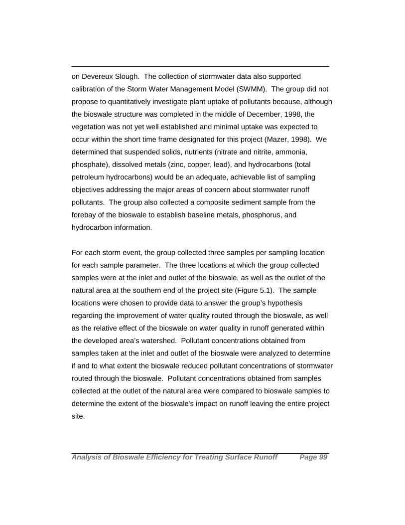
Analysis of Bioswale Efficiency for Treating Surface Runoff Page 99
on Devereux Slough. The collection of stormwater data also supported
calibration of the Storm Water Management Model (SWMM). The group did not
propose to quantitatively investigate plant uptake of pollutants because, although
the bioswale structure was completed in the middle of December, 1998, the
vegetation was not yet well established and minimal uptake was expected to
occur within the short time frame designated for this project (Mazer, 1998). We
determined that suspended solids, nutrients (nitrate and nitrite, ammonia,
phosphate), dissolved metals (zinc, copper, lead), and hydrocarbons (total
petroleum hydrocarbons) would be an adequate, achievable list of sampling
objectives addressing the major areas of concern about stormwater runoff
pollutants. The group also collected a composite sediment sample from the
forebay of the bioswale to establish baseline metals, phosphorus, and
hydrocarbon information.
For each storm event, the group collected three samples per sampling location
for each sample parameter. The three locations at which the group collected
samples were at the inlet and outlet of the bioswale, as well as the outlet of the
natural area at the southern end of the project site (Figure 5.1). The sample
locations were chosen to provide data to answer the group’s hypothesis
regarding the improvement of water quality routed through the bioswale, as well
as the relative effect of the bioswale on water quality in runoff generated within
the developed area’s watershed. Pollutant concentrations obtained from
samples taken at the inlet and outlet of the bioswale were analyzed to determine
if and to what extent the bioswale reduced pollutant concentrations of stormwater
routed through the bioswale. Pollutant concentrations obtained from samples
collected at the outlet of the natural area were compared to bioswale samples to
determine the extent of the bioswale's impact on runoff leaving the entire project
site.

Analysis of Bioswale Efficiency for Treating Surface Runoff Page 100
During the course of any individual rain event, the critical time period for sample
collection is the “first flush” which occurs within the first 10 to 60 minutes,
depending upon rainfall intensity of the storm event. The first flush contains the
majority of the pollutants in the stormwater runoff generated during the rain event
(Line, et al., 1997). Samples collected several hours after the rain begins are not
representative of the total concentrations of pollutants contained in the
stormwater runoff. Several samples must be collected during the rain event in
order to calculate Event Mean Concentration values (U.S. EPA, 1983). The
bioswale group project therefore collected three samples at each location for
each storm event. The first set of samples was collected at the inlet to the
bioswale 10 minutes after runoff was first observed at this location. The next two
samples at this location were collected at thirty-minute intervals. This allowed for
the “first flush” to be represented in the sampling.
Analysis of Bioswale Efficiency for Treating Surface Runoff Page 101

Analysis of Bioswale Efficiency for Treating Surface Runoff Page 102
The time of collection for the first sample at the bioswale outlet was determined
using the detention time of water routed through the bioswale during the storm
event. Detention times were calculated based on flow estimates obtained in the
field during the storm event. For example, if the detention time was determined
to be 15 minutes, the first sample collected at the bioswale outlet was collected
15 minutes after the first sample was collected at the bioswale inlet.
The bioswale group project collected stormwater samples for four rain events.
The first set of samples was collected on 11/7/98. Because the bioswale was not
yet completed and flow was not being routed through the structure, the group
collected runoff samples from the K-Mart parking lot (Figure 5.1). Runoff
collected from this area is routed through the completed bioswale, and was
expected to represent typical first flush concentrations of stormwater runoff from
the first major rain event of the season after several months of pollutant loading.
The next rain event the group attempted to sample occurred on 1/19/99, but the
group discovered that although the structure was completed, stormwater runoff
was not yet being routed through the bioswale and so could not collect
stormwater samples. Just before the beginning of this rain event, the group
collected a composite sediment sample from the forebay of the bioswale to
establish baseline soil conditions prior to any additional loading (the sample was
analyzed for total petroleum hydrocarbons, total phosphorus, and trace metals).
The other three sampling events occurred in January and February 1999 (Table
5.1), with the length of time between each storm event varying, thus affecting the
amount of pollutant loading. In Table 5.1, total rainfall is the amount of rain
occurring in each rain event, and does not represent only the amount of rainfall
during sampling. Each time a sample was collected, water heights were also
measured in order to establish flow discharge necessary for the calculation of
pollutant Event Mean Concentrations (EMCs), a flow-weighted measure of
pollutant concentration for a given storm event.

Analysis of Bioswale Efficiency for Treating Surface Runoff Page 103
Table 5.1Date, Location and Total Rainfall of Each Sampling Event
Date Location Rainfall (inches)November 7, 1998 K-Mart Parking Lot 0.32January 24, 1999 Bioswale 0.24January 31, 1999 Bioswale 0.47February 9, 1999 Bioswale 0.70
All samples were collected in polyethylene containers (for nutrients, metals, and
total suspended solids) or amber glass bottles (for total petroleum hydrocarbons)
and refrigerated before being transported to the analytical laboratory in iced
coolers. All analyses were conducted according to standard EPA methods as
outlined in Standard Methods (Clesceri, 1989). The project developer, Wynmark
Company, provided a portion of funding for analyses. Additional grant funds from
the University of California Toxic Substances Research and Teaching Program,
Coastal Component were used to purchase supplies and laboratory analysis
services for a portion of our field sampling efforts.
It is important to note that at the time of all sample collection, the bioswale
structure was complete but vegetation throughout the structure had not been
established. While the primary treatment process for pollutant removal in the
bioswale is gravitational settling and removal of particulates, vegetation is
expected to provide additional physical filtration of stormwater and dissolved
pollutant uptake. The following chemical sampling results are therefore
considered a preliminary data set that does not completely reflect all the
processes the bioswale and its plants will eventually exert on stormwater runoff.
5.3 Chemical Sampling Results
Results of chemical analyses of stormwater samples collected at K-Mart on
11/7/98 are presented in Table 5.2. Total dissolved solids and chloride were not
routinely measured for every sampling event of this project, but are included here

Analysis of Bioswale Efficiency for Treating Surface Runoff Page 104
to provide potential levels of contaminant loading prior to the first major rain
event of the winter season.
Table 5.2Summary of Event Mean Concentration (EMC) Values (milligrams per liter)
for Selected Pollutants of Samples Collected at the K-Mart Location.
EMCs for nutrients, total suspended solids, and dissolved metals are
summarized in Table 5.3. No samples were collected for analysis from the outlet
of the natural area on 1/31/99, because the rain event was too small to generate
flow through the entire system. Flow measurements are summarized for each
sampling event in Appendix D.
Date Pollutant EMC (mg/L)11/7/98 TPH 6
" Total P as Phosphate 30" Nitrate + Nitrite 3" Lead 0" Total Suspended Solids 24" Total Dissolved Solids 1209" Chloride 329

Analysis of Bioswale Efficiency for Treating Surface Runoff Page 105
Table 5.3Summary of Event Mean Concentration (EMC) Values (milligrams per liter)
for Selected Pollutants for Three Rain Events.
5.4 Discussion of Chemical Results
Results for all field sampling conducted during the course of this group project
are preliminary. Interpretation of water quality field data is necessarily cautious
when based on only a few sampling events that had variable rain intensities and
different periods of pollutant loading prior to rain events. Similar cautions apply
to the soil analysis results that are presented for a single composite soil sample.
Date Pollutant Bioswale Inlet Bioswale Outlet Natural Area Outlet1/24/99 Total Petroleum Hydrocarbons nd nd nd1/31/99 NM NM NM2/9/99 nd nd nd1/24/99 Total P as Phosphate NM NM NM1/31/99 12 7 NM2/9/99 5 6 5
1/24/99 Nitrate + Nitrite (NO3-N +NO2-N) nd nd nd1/31/99 70 50 NM2/9/99 17 24 181/24/99 Ammonia (NH3-N) NM NM NM1/31/99 157 132 NM2/9/99 130 124 1321/24/99 Copper (dissolved) nd nd nd1/31/99 0.01 0.01 NM2/9/99 0.02 0.00 nd
1/24/99 Lead (dissolved) NM NM NM1/31/99 0.10 0.03 NM2/9/99 nd nd nd1/24/99 Zinc (dissolved) nd nd nd1/31/99 0.042 0.031 NM2/9/99 0.019 0.023 0.0101/24/99 Total Suspended Solids 28 47 221/31/99 346 495 NM2/9/99 269 233 219
nd = not detectedNM = not measured

Analysis of Bioswale Efficiency for Treating Surface Runoff Page 106
Several samples collected on 1/31/99 demonstrated apparent differences in
Event Mean Concentrations between the bioswale inlet and outlet. Total
phosphorus, nitrate plus nitrite, ammonia, lead, and zinc all appeared to have
decreased in samples collected at the bioswale outlet, while total suspended
solids appeared to have increased relative to inlet concentrations. For samples
collected on 2/9/99, nitrate plus nitrite and total suspended solids appeared to
have decreased at the outlet compared to their inlet concentrations. A Student’s
t-test revealed, however, that none of the differences in Event Mean
Concentration were statistically significant (Table 5.4). In no case would we
reject the null hypothesis (H0) that the means are equal. This result is not
unexpected because the low number of samples results in low degrees of
freedom. According to this statistical analysis, the apparent decreases in
pollutant concentrations cannot be attributed to bioswale processes, but rather
are interpreted as the variability between individual sample results at any given
sample location.
Table 5.4Summary of Student’s t-test of Apparent Differences in Event Mean
Concentrations for Samples from Bioswale Inlet and Outlet (Samuels, 1986)
Date Parameter n d.f. p(0.05) t-statistic Reject Ho?1/31/99 Total P 4 3 3.182 2.192 no
NO3 + NO2 4 3 3.182 2.805 noNH3 4 3 3.182 1.471 noLead 4 3 3.182 0.084 noZinc 4 3 3.182 0.012 noTSS 4 3 3.182 -1.211 no
2/9/99 NO3 + NO2 3 2 4.303 -2.817 noTSS 3 2 4.303 1.882 no

Analysis of Bioswale Efficiency for Treating Surface Runoff Page 107
5.4.1 Water Quality Criteria
Table 5.5 summarizes water quality criteria for pollutants addressed in this study,
as established by the U.S. EPA (1986). Some criteria have specific numerical
values, while others are narrative. Quality criteria are presented for both marine
and freshwater environments. Devereux Slough is usually brackish, with
freshwater inputs being modified by seasonal inputs of seawater when the slough
opens to the ocean (de la Garza and Ryan, 1998). The bioswale group project
did not address specific potential impacts on aquatic inhabitants of Devereux
Slough. de la Garza and Ryan (1998) asserted that concentrations of
stormwater pollutants could potentially exceed the EPA criteria for high end
estimations of pollutant loading. Their high-end estimates of pollutant loading did
not account for the stormwater management measures installed at Camino Real
that reduce pollutant loads between their sources and their ultimate destination in
Devereux Slough.
We observed that all samples analyzed for total petroleum hydrocarbons were at
non-detectable levels, and can be interpreted as a positive result of the
installation of Fossil Filters® at catch basins upstream of the bioswale. At the
same time, the full extent of hydrocarbon loading onto parking lots has not yet
occurred since major portions of the stores and parking lots are still under
construction. There are no consistent trends in the results for total suspended
solids, and this is most likely due to the incomplete vegetated state of the
bioswale that existed at the time of sampling compounded by erosion of the
banks of the bioswale (Figure 5.2).

Analysis of Bioswale Efficiency for Treating Surface Runoff Page 108
Figure 5.2Erosion of Bioswale Banks
Table 5.5U.S. EPA Water Quality Criteria (U.S. EPA, 1986)
Concentrations ug/LFresh Fresh Marine MarineAcute Chronic Acute Chronic
Pollutants Criteria Criteria Criteria CriteriaCopper 18* 12* 2.9 2.9Lead 82* 3.2* 140 5.6Nitrates NE NE NE NEPetroleum Hydrocarbons (Oil and Grease) narrative statementPhosphorus NE NE NE NESuspended Solids narrative statementZinc 120* 110* 95 86
NE = Not Established* = Hardness-dependent criteria (100 mg/L used)
Acute effects are short-term lethal effects that occur within 4 days of exposure.Chronic effects occur over a longer period and include changes in feeding, growth, metabolism, or reproduction in addition to eventual death.Petroleum Hydrocarbons (as Oil and Grease): Domestic water supplies should be "virtually free from oil and grease," particularly from the tastes and odors that emanate from petroleum products.Suspended Solids: Criteria are established for solids and turbidity primarily due to their effect on productivity by reducing light penetration. The criterion for suspended solids is that the depth of the compensation point for photosynthetic activity should not be reduced by more than 10 percent from its seasonally established norm.

Analysis of Bioswale Efficiency for Treating Surface Runoff Page 109
5.4.2 Sediment Quality Criteria
Sediment quality criteria standards are even less well established than are those
for water.
Establishment of sediment criteria standards has long been a goal of the U.S.
EPA, who recently published the Contaminated Sediment Management Strategy
(1998). This document does not provide specific soil quality parameters, but
outlines a systematic approach to sediment monitoring and assessment. The
EPA approach discusses several steps deemed necessary for the effective
establishment of a nationwide management strategy, one of which is the
establishment of quality criteria for the protection of benthic organisms.
Baudo, et al., (1990) presented standards that are currently in use, as well as
proposed sediment contaminant standards for a variety of pollutants. Table 5.6
is a compilation of proposed sediment quality criteria and includes the forebay
composite soil sample results for comparison. The soil quality criteria represent
best estimates of the lowest effect levels of contaminants on benthic organisms.
Of the pollutants listed in Table 5.6, total petroleum hydrocarbons in the forebay
are noticeably higher than the recommended standard of 100 ppm. Total
phosphorus is also high, along with some of the metals such as nickel and zinc.
The three metals of highest environmental concern (copper, lead, and zinc) are
all present in the forebay soil, although their concentrations do not exceed
recommended criteria at this point. The results from a single soil sample do not
reliably establish the pollutant levels in the forebay, and additional samples are
necessary to establish a more accurate picture of mean pollutant values and their
variability. We recommend further sediment sampling in the forebay and other
parts of the bioswale to better establish the present soil conditions prior to
additional loading. A major reason for performing additional soil analysis is that if

Analysis of Bioswale Efficiency for Treating Surface Runoff Page 110
contaminant levels exceed quality criteria, this information may be required to
establish the amount of cleanup necessary before forebay soil disposal.
Table 5.6Summary of Recommended Sediment Quality Criteria and Forebay Sample Results.
5.5 Transport and Fate of Contaminants at Camino RealA logical extension of the chemical analysis addresses the transport and fate of
pollutants. Figure 5.3 presents a conceptual model of potential reservoirs and
transport routes for pollutants at Camino Real. Pollutants may remain
sequestered in the bioswale forebay, but larger flow events have the potential to
re-suspend sediment and disperse pollutants to the bioswale backbay and
natural area. Plants in the bioswale can contribute to pollutant uptake, but the
maximum uptake capacity of plants and the length of time required for uptake
limit this process.
Ontario Ministry of Environment andWisconsin Dept. of Natural Resources Forebay Composite Results
Sediment Quality Critera Constituent mg/kg (ppm) mg/kg (ppm)TPH 100 230Total P as Phosphorous 600 700Total P as Phosphate 2100Antimony ndArsenic 10 ndBarium 61Beryllium ndCadmium 1 ndChromium 100 16Cobalt 25 6.9Copper 100 7.8Lead 50 5.7Mercury 0.1 ndMolybdenum 4 ndNickel 100 95Selenium 2 ndSilver 0.5 ndThallium ndVanadium 16Zinc 100 44nd = not detectedSource: Baudo, et al., 1990

Analysis of Bioswale Efficiency for Treating Surface Runoff Page 111

Analysis of Bioswale Efficiency for Treating Surface Runoff Page 112
This page intentionally left blank

Analysis of Bioswale Efficiency for Treating Surface Runoff Page 113
6.0 Biological Considerations
The bioswale and the natural area represent a major portion of the remaining
open space on the Camino Real Development site. With the construction of the
development, a considerable amount of open space, considered to be a
significant visual resource, was lost (Camino Real Project EIR, 1997). Therefore,
the bioswale is not only a means of providing runoff treatment, but also acts to
visually enhance the area. In the Enhancement and Management Plan for
Camino Real (1997) one of the stated functions for the bioswale is “on-site
replacement of riparian habitat”. The Army Corps of Engineers defined the
bioswale as wetland replacement, and a such provides an open vegetated area
for various animal species such as, birds, frogs and possibly fairy shrimp (an
endangered species associated with local vernal pools) as suggested by the lead
biologist (Bomkamp, personal communication). It is expected that prolonged
periods of ponded water will occur near the outlet of the bioswale due to the built
in depression and relatively impermeable soil.
The natural area at the southern border of the development site works along with
the bioswale to filter pollutants. All runoff, even that bypassed around the
bioswale, is routed through the natural area before it exits the site. The natural
area, therefore, acts as a vegetated continuation of the bioswale and performs
many of the same functions. It is also important in enhancing the project site
while providing additional wildlife habitat. The Environmental Impact Report
designates this “willow grove” as an Environmentally Sensitive Habitat, classified
under Riparian Woodlands/Corridor. This area was essentially left intact with
some of the undergrowth and invasive species removed and the addition of
native plantings both in the natural area and around the perimeter.

Analysis of Bioswale Efficiency for Treating Surface Runoff Page 114
6.1 Phytoremediation
Phytoremediation is the use of plants to remediate polluted water or soil. The
plants in the bioswale at Camino Real are expected to significantly increase
degradation of pollutants by chemical alterations occurring in the root zone, or to
contribute to pollutant decrease by physical uptake. Plants, particularly wetland
species, have been used extensively to treat municipal and industrial
wastewater, but the use of plants to treat in situ contaminated zones has only
recently come into use (Anderson & Coats, 1994). Studies have shown
considerable promise towards increasing use of plants to treat some polluted
sites, but more information needs to be acquired. The bioswale’s purpose is to
treat pollutants as they arrive and accumulate, not to clean an already
contaminated site. Thus phytoremediation is being used to reduce the rate of
possible long-term chemical build up, as well as minimize pollutant loading off-
site with potential damages to Devereux Slough.
Plant species play a large role in pollutant uptake ability, with many plants able to
degrade or uptake certain pollutants occurring at various rates (Anderson 1994).
Much of the recent research is focusing on creating new breeds and hybrids that
will be able to accumulate more pollutants over shorter time intervals. Plants
also assist in the physical removal of particles by acting as barriers to the water
flow; this decrease in flow speed enhances settling of suspended sediment.
Some uptake of pollutants is possible on above ground plant surfaces, this
occurs mostly with organic pollutants such as PAHs (polycyclic aromatic
hydrocarbons) (Simonich and Hites, 1995). For example, plant accumulation of
some organic pollutants can occur through reactions between air and leaf, as
well as from deposition of particles out of the water column onto exposed
surfaces.

Analysis of Bioswale Efficiency for Treating Surface Runoff Page 115
The majority of phytoremediation occurs in the root zone of plants – the
rhizosphere. The rhizosphere represents a microenvironment where bacteria
and fungi, along with plant roots, form a unique community that has the potential
for detoxification of hazardous compounds. In natural plant ecosystems,
microbial communities are found in symbiotic relations with plants. The presence
of plants increases the abundance of microorganisms in the rhizosphere. This
increase is commonly 5-20 times greater than in non-vegetated soils, and can be
as high as 100 or more times (Kruger, 1997). The plant provides exudates to the
microbial community, which stimulates activity and often leads to a build up of the
organic carbon content in the soil, while the plant receives, in turn, mineral
nutrients.
Plants exude a variety of compounds, both organic and inorganic, to stimulate
microbial communities in their root area including sugars, amino acids,
carbohydrates, acetates, carbon, esters, benzene derivatives, enzymes and
essential vitamins. These exudates can mobilize essential nutrients from the
soil, and act as chemo-attractants, thus stimulating bacterial activity and altering
toxicant sorption, bioavailability and leachability. Fungi are the second most
prevalent group of microorganisms in the soil, and grow in association with plant
roots and provide unique enzymatic paths for the degradation of organics not
available through bacteria alone. Mychorrizal fungi are especially important in
the rhizosphere for a wide range of herbaceous and woody plants, and can
improve plant success in nutrient or water limiting conditions. Though bacteria
and fungi can catabolise (break down) many of the same contaminants, they do
so by different mechanisms. Which process is more prevalent depends on the
soil properties and its constituents. Exudates from the plant as well as the cell
wall mechanisms of the plant root vary with plant species. The cell walls of the
plant root are a source of fixed, non-diffusible charges that may adsorb particles
in the rhizosphere and make them less bioavailable. Bioavailability is defined as
Analysis of Bioswale Efficiency for Treating Surface Runoff Page 116
the amount of a compound present in soil solution or readily exchanged off of
system surfaces.
6.1.1 Phytoremediation Mechanisms of Organic Contaminants
Plants remove organic contaminants through two mechanisms: (1) direct uptake
and accumulation of contaminants, and (2) degradation by stimulating the
rhizosphere microbial communities through the use of exudates and enzymes
from the plant. There are several important plant factors that play a role in the
capacity of the plant to take up contaminants, such as: the plant species, age,
vigor of rooted plant, soil properties and climatic conditions. The majority of the
microbes are composed of bacteria, but there is also usually a large fungi
population. Just as plant uptake is influenced by many factors, the microbial
community in the soil also depends on a variety of soil parameters, such as:
temperature, aeration, salinity, texture and nutrient availability. Especially critical
for microbes are moisture, temperature and oxygenation.
Schnoor, et al., (1995) found hybrid poplars to be particularly effective at treating
soils with organic contaminants. Poplars were used at several study sites, either
alone or in conjunction with other plants, to degrade contaminants such as
atrazine, chlorinated solvents, organics (mostly nitrate and phosphate), and
metals. Poplars planted directly on top of landfills flourished and maintained
growth even after several years, they immobilized organics in the soil and added
to soil stability thus decreasing soil erosion. Plants with relatively deep roots
and/or dense root mass can take up large volumes of water, thus decreasing
downward percolation of water, along with associated pollutants, into the water
table.

Analysis of Bioswale Efficiency for Treating Surface Runoff Page 117
The accessibility of organic contaminants to plants varies greatly. Plants are
highly efficient in the uptake of hydrophobic organic compounds. Hydrophobicity
is expressed as the log of the ‘octanol-water partitioning coefficient’ Kow, where
contaminants with high Kow can show significant root uptake. However, in
organic-rich or highly textured soils, hydrophobic compounds may sorb strongly
to soil particles and become unavailable for root adsorption. Once adsorbed,
plant tissues sequester organic contaminates or volatize, metabolize, and
mineralize the chemicals to carbon dioxide, water and chlorides (Suthersan,
1997).
6.1.2 Phytoremediation Mechanisms of Heavy Metals
Most heavy metals have several physical and chemical forms in the soil. Metals
may be found dissolved in the soil solution, adsorbed to plant roots, adsorbed to
insoluble inorganic matter, bonded to ion exchange sites on inorganic soil
constituents, precipitated as solids, or attached to soil biomass. Plant roots help
to prevent the erosion of soils and the metal contaminants associated with them,
as well as engage in uptake of metal contaminants. Metals often remain in the
roots of the plant, and to a limited degree are translocated to aboveground plant
parts. Some species known as hyperaccumulators have been shown to uptake
large quantities of metals without toxic side effects.
The amounts of metals in stormwater runoff available for biological uptake are
closely approximated by the percentage of dissolved metals within the runoff.
Zinc, cadmium, and copper are highly available for uptake, while lead, iron, and
aluminum are frequently bound to particles and less available (Sansalone and
Buchberger, 1997). Metals uptake varies widely by plant species and levels of
exposure. Further investigation is required to make qualitative uptake predictions

Analysis of Bioswale Efficiency for Treating Surface Runoff Page 118
for bioswale vegetation. Biological uptake may facilitate metals introduction into
the food web.
Plants have been shown to accumulate heavy metals, as well absorb and
metabolize a variety of organic chemicals. Table 6.1 lists contaminants known to
be suitable for phytoremediation.
Table 6.1Contaminants Suitable for Phytoremediation
Moderately HydrophobicContaminants
Excess Nutrients Heavy Metals
benzene nitrate chromiumtoluene ammonium cadmiumethylbenzene phosphate zincXylenes leadChlorinated solvents mercuryPAH’s* arsenicNitrotoluene nickelAmmunition wastes copper
silver*Polycyclic aromatic hydrocarbons
Source: Suthersan, 1997
6.1.3 Plant Selection for the Bioswale
All former vegetation has been removed from the area where the bioswale is now
located. The planting of the bioswale is divided into four areas: the forebay, the
backbay, the dam (separating the forebay from the backbay), and the banks.
Plants in each area were selected according to expected soil moisture levels and
degree of inundation. Table 6.2 summarizes the plants used in the Camino Real
bioswale.

Analysis of Bioswale Efficiency for Treating Surface Runoff Page 119
Table 6.2Bioswale Plant List
Planting Area Scientific name Common Name
Forebay Eleocharis palustris Spike RushAnemopsis californica Yerba ManzaLilium pardolinum Water Lilly
Backbay Scirpus maritimus Bull RushScirpus californica Bull Rush
Distichlis spicata Salt GrassJuncus patens Common RushCyperus eragrostis Common CyprusJuncus phaeocephalus Brown Headed
Creeping Rush
Berm Artemesia californica California SagebrushBaccaris pilularisDiplacus duranliucus MonkeyflowerElymus condensatus Giant Ryegrass
Bank Plantanus racemosa Western SycamorePopulus fremonti Fremont CottonwoodAcer negundo BoxelderQuercus agrifolia Live OakPrunus lyonii Catalina CherryGeteromeles arbutifoliaRhus integrifolia Lemonade BerryNassella pulchra Purple NeedlegrassBerberis nevinii BarkberryRubus ursinus California BlackberryArtemesia douglasii MugwortRosa californica California Wild Rose
6.1.4 Plant Specifics
There is a scarcity of information regarding the specific plant species in the
bioswale and their potential pollutant uptake; this is probably due to the lack of
similar water treatment systems in southern California. Selection of plant species
was based on two criteria: that they are native to the area and will survive given

Analysis of Bioswale Efficiency for Treating Surface Runoff Page 120
the expected soil conditions. Plants in the main channel of the backbay were
selected for their ability to survive up to a month of standing in ponded water.
Some work has been done looking at plants of the same genus as the plants in
the bioswale, but of different species. While this may provide an indication of
general plant functioning, caution should be used when extrapolating plant
behavior among different species. This information can provide clues to the
success of pollutant uptake within a given plant, but ongoing research should be
conducted to analyze actual uptake ability for each plant within the bioswale.
Following are some examples of research in this area that potentially indicate
how plants in the bioswale will perform.
6.1.5 Synopsis of Research on the Uptake Ability of Various Plants
Rejmankova and Bayer (1995) analyzed two species of the Scirpus genus,
Scirpus acutus and Scirpus californicus (the bioswale has Scirpus maritimus).
These two species behaved similarly in regards to their metal uptake abilities,
with most of the metals remaining in the roots and not being translocated to the
shoots to any significant degree. In the author’s heavy metal analysis, none of
the five species examined had significant uptake of metals in above ground
growth, with significant accumulation of metals only occurring in the roots. Their
analysis was based on two natural (non-polluted) wetlands that were used as
control sites and compared to four other treatment sites, with all locations in
either Davis or Fairfield, California. Both Scirpus acutus and Scirpus californicus
were found to allocate more of their biomass into their below-ground structure
when water levels are periodically drawn down, as opposed to continual flooding.
This could affect pollutant uptake since as far as metals are concerned, most of
the accumulation is in the root zone. In general these two species grow well in a

Analysis of Bioswale Efficiency for Treating Surface Runoff Page 121
wide range of water depths and nutrient concentrations. They can survive
occasional deep flooding as well as droughts, and are highly productive.
Breen, Mag and Seymour (1994) studied a similar system to the bioswale, which
they call a flood-retarding basin, located in Melbourne, Australia. They also note
that the majority of urban runoff consists of pollutants adsorbed onto mineral
particulates, and thus one of the key roles of the plants is to remove these
particles from the water column. This study, as well as others including data
from King County, WA, deem that optimum performance in such a water
treatment system is enhanced by a wide variety of species. Since each plant
performs differently, and especially since data on pollutant uptake is limited,
there is a better chance that performance will increase with a variety of plant
species as opposed to only several. The only exception to this may be plants
known as “hyperaccumulators”. Preliminary research is being conducted on
special breeds that uptake pollutants, mostly metals, at several orders of
magnitude higher than other observed plants (Cunningham and Ow, 1996).
Also, a variety of plant species is also helpful at the beginning stages of the
bioswale (or similar system), since inevitably some plants will do well while
others will die.
The Australian basin uses some Juncus species in areas that are frequently
inundated, which are similar to wet zones in the backbay that contain 2 species
of Juncus. Though the authors do not provide any data on pollutant uptake
ability by the plants, they make recommendations about which species would be
appropriate given the hydrologic conditions of the area. They also recommend
Eucalyptus trees in areas that occasionally are inundated, such as the higher
elevations in the backbay or even on the lower slopes of the bioswale. Even
though Eucalyptus trees grow well in the Santa Barbara area, they are not native
and are not recommended for a small site such as the bioswale where they could
easily prohibit other growth.

Analysis of Bioswale Efficiency for Treating Surface Runoff Page 122
The King County Surface Water Design Manual (1997) lists acceptable plants for
a “wet biofiltration swale”, which is similar to the Camino Real bioswale. This list
includes several species of Eleocharis, Juncus tenuis, Scirpus acutus and
Scirpus microcarpus, reflecting similar species planted in the bioswale. It notes
that cattails (Typha latifolia) are not appropriate for most wet swales due to the
plant’s dense and clumping growth habit, which prohibits water filtration. Also,
typical wetland vegetation does not respond well to high velocity flows, which
cause the plants to fall over and are subsequently unable to return upright. This
problem is addressed in the bioswale where flows in the backbay are gentle.
Kemp and Cunningham (1980) studied Distichlis spicata, which is planted in the
backbay. This particular grass occurs over a wide geographic area, thus showing
itself to be fairly hardy and well able to adapt to different environments. D.
spicata is shown to be highly salt-tolerant, which is a possible concern within the
bioswale. The event mean concentration (EMC) of chloride in stormwater
samples from the bioswale (1/24/99) ranged between 5 and 12 mg/L, with
chloride concentration providing a good indicator of total salt levels. The sample
series taken from the runoff of K-Mart parking lot exhibited a higher chloride
concentration, with an EMC of 329 mg/L. This sample was taken after a long dry
period and indicates a longer period of pollutant buildup. Kemp and Cunningham
(1980) showed that moderate to high levels of salinity (14.6-29.3 mg/L NaCl)
significantly reduced net photosynthesis given warm temperatures and bright
light conditions, which would be the dominant conditions for the bioswale.
Therefore, even though plants such as D. spicata can survive periods of high
salinity, growth rates are diminished and decrease pollutant uptake. Studies
show that the evapotranspiration rate plays a significant role in pollutant
degradation (Burken & Schnoor, 1996). The ability of the plant to transport
oxygen to the soil stimulates rhizome activity and degradation of pollutants.

Analysis of Bioswale Efficiency for Treating Surface Runoff Page 123
6.1.6 Limits of Phytoremediation
Despite advances in technology, additional information is needed to assess the
various plants and their potential to decrease or transform pollutants either by
direct uptake or by their contributions to the soil to enhance microbial activity.
The process of soil transformation through phytoremediation is still slow for most
plant species, which has a direct effect on best management practices, policy
regulations, and ultimately remedial costs. This is especially true for hydrophobic
pollutants that bind tightly to soil particles and thus require a long time to
remediate. One of the arguments in favor of phytoremediation is that costs are
substantially lower for in situ treatments as opposed to transporting material
offsite, but this benefit must be weighed against the length of time needed for
treatment.
According to Cunningham & Ow (1996), research on future technologies is
focusing on developing new hybrids, with new genetically modified plants able to
uptake more pollutants and at a faster rate. They envision a new valuation
system that selects plants “based on what they absorb, sequester, destroy and
tolerate”. Several aspects of a plant structure could be improved, such as
deeper roots and increased root density. Deeper roots would allow the plant to
filter pollutants further down in the soil column, while increased root density may
make extraction more efficient. Many studies have focused on organic pollutant
uptakes, which appears to happen more easily than accumulating metals into the
plant structure. Again, some research is being directed towards analyzing metal
uptake, for example some plant mutations have exhibited a 10 to 100-fold
increase in metal accumulation compared to their non-mutant counterparts
(Cunningham & Ow, 1996 ).
It is still unclear if a plant accumulates significant portions of pollutants in leaves
and thus re-releases contaminants during litter fall; this probably varies with the

Analysis of Bioswale Efficiency for Treating Surface Runoff Page 124
type of plant. Studies so far have not emphasized this aspect and it does not
appear to be of high concern, but still merits further investigation. Whether or not
this is a problem has ramifications for ensuing biological consumption of toxic
materials as well as re-mobilizing the pollutant. It is also uncertain whether the
plants are most important for their actual uptake abilities, or whether the release
of exudates and subsequent stimulation of the rhizosphere is their primary role.
It is clear that the plants in the bioswale will aid in the removal of soil particles
and their associated contaminants and will contribute to contaminant degradation
in the soil. The uncertainty lies in knowing to what degree these processes
contribute to the overall removal of contaminated constituents from the runoff at
the Camino Real development.
6.1.7 Vegetation Establishment and Growth
The successful establishment and growth of plants within the bioswale is key to
the achievement of its water quality goals. Plant species have been selected for
use in the bioswale based on their ability to thrive in the hydrologic regimes
anticipated to be present in the bioswale. Given the high investment of time and
effort in planting, successful establishment of vegetation is quite likely. The long-
term growth and community composition of vegetation within the bioswale is
dependent on hydrologic regimes, access to sunlight, soils, and vegetation
community dynamics.
Plants within the bioswale will experience a variety of hydrologic conditions
depending on season, location within the bioswale, Camino Real site usage, and
management intervention. The strong seasonality of precipitation (in Santa
Barbara precipitation comes predominantly from November to March) will result
in a bioswale that is frequently ponded or inundated in the winter and significantly
drier in the summer. The topography within the bioswale will strongly influence

Analysis of Bioswale Efficiency for Treating Surface Runoff Page 125
the hydrologic regime to which plants are exposed. The bioswale is
topographically separated into wet, mid, top, and upper slope zones; forebay and
backbay; and micropool. The bioswale is expected to receive some water daily
from watering and washdowns on the Camino Real Shopping Center (Yean,
personal communication). Since construction is not completed, the amount and
variation of daily flows is not yet known. Direct watering of the bioswale may be
required to maintain plant health through extended dry periods. In anticipation of
extended dry conditions, sprinklers have been installed in the bioswale.
Access to sunlight is a critical component in the growth and community
composition of plants within the bioswale. Moderate to high vegetation density
requires abundant sunlight (Mazer, 1998). Trees planted within the bioswale will
increasingly shade areas of the bioswale over time. The sandy clay soil within
the bioswale is suitable for all of the plants selected for use in the bioswale
(Bomkamp, personal communication). The initial soil conditions will favor some
plants, and sedimentation and concentration of contaminants will change the soil
conditions that will favor other plants over time.
Since the controlling factors of vegetation growth are expected to vary over time,
the vegetation community composition will also vary as. The variety of plants
initially planted within the bioswale provides numerous and significantly different
plant species which will attempt to colonize the bioswale. Ultimately, the
vegetation community will progress towards one that is dominated by those
species most suited to the particular environmental conditions within the
bioswale.

Analysis of Bioswale Efficiency for Treating Surface Runoff Page 126
This page intentionally left blank

Analysis of Bioswale Efficiency for Treating Surface Runoff Page 127
7.0 Economic and Regulatory Considerations
7.1 Why a Bioswale?
The Camino Real development considered several factors in the choice of
stormwater treatment system. In addition to concerns regarding water quality,
permitting required that the developer address flood containment capacity and
mitigate for wetland loss. This section discusses options that were considered for
stormwater treatment, which were narrowed to the choice of a bioswale due to its
additional benefits addressing flood containment and wetland mitigation.
The Environmental Impact Report (EIR) for Camino Real mandated the use of oil
and grease traps, or equivalent, which resulted in the installment of Fossil Filters® at
each catch basin. This type of oil and grease trap provides removal of
hydrocarbons, suspended sediment, and floatable debris. An alternative option was
to use the Stormceptor , which provides the same water treatment as Fossil
Filters®, but has a larger pollutant storage capacity. Following is a description of
both Fossil Filters® and Stormceptors .
Fossil Filters® are trough structures installed under the grates of all runoff catch
basins (Figure 7.1). They are principally designed to trap petroleum hydrocarbons
and associated pollutants, while still allowing unrestricted flow of water into drainage
pipes. They conform to EPA standards under the National Pollutant Discharge
Elimination System (NPDES) program and are considered to be economically
feasible and fall under the definition of Best Available Technology. These structures
are made in a variety of shapes and sizes, and should catch all flow directed towards
the catch basin. The non-hazardous adsorbent material in each Fossil Filter®,
known as Amorphous Alumina Silicate, traps the hydrocarbons and remains effective
until 50% or more of the filter material is covered with pollutants. Minimum
recommended maintenance for each structure is three cleanings and one change of

Analysis of Bioswale Efficiency for Treating Surface Runoff Page 128
filter material annually. To ensure proper functioning, regular maintenance of the
structures must include removal of large debris to allow unrestricted water passage.
The Stormceptor is a subsurface chamber made of precast concrete or
fiberglass components that are assembled and installed in either new or existing
storm sewers. The Stormceptor is designed to treat more than 80% of all storm
events (Stormceptor Corporation, 1996) and directs stormwater flow into an
upper bypass chamber, where a u-shaped weir diverts the flow down to the main
treatment chamber (Figure 7.2). In this lower chamber hydrocarbons and
floatable debris rise to the top and become trapped, while sediment settles to the
bottom. The main advantage of the Stormceptor is that during high flow
events, previously collected pollutants will not be scoured from the device. High
flow volumes will simply pass over the u-shaped weir and continue through the
bypass chamber to the downstream stormwater system. Maintenance of the
Stormceptor consists of measuring accumulated sediment depths and
subsequent removal of accumulated solids through the manhole access with a
vacuum truck. Stormceptor® units are available in a variety of sizes, with main
treatment chamber capacities ranging from 450 to 7400 U.S. gallons. Even the
largest Stormceptor® unit, however, is only expected to treat a maximum
impervious drainage area of 5.5 acres for 80% removal of TSS (Stormceptor®
Corporation, 1996).

Analysis of Bioswale Efficiency for Treating Surface Runoff Page 129
Figure 7.1
Schematic Design of a Fossil Filter
Source: KriStar Enterprises, Inc.

Analysis of Bioswale Efficiency for Treating Surface Runoff Page 130
Figure 7.2Schematic Design of Stormceptor® Stormwater Treatment Device.
Manhole cover at top gives rough idea of scale.
Source: Stormceptor® Corporation, 1996.
The guidelines about the maximum impervious area a single Stormceptor® unit
can effectively treat, as well as flow restrictions, raised questions about the use
of the Stormceptor®. It became clear that without a large number of units, the
expected runoff volumes of major storms could not effectively be processed at
the Camino Real development. The same number of Stormceptors as Fossil
Filters® would have been required, and the large price difference eliminated
Stormceptors® from further consideration. Instead, thirty Fossil Filters® were
installed at all major catch basins. Including material and labor, construction cost
for each Stormceptor® is approximately $150,000 and $225 for each Fossil

Analysis of Bioswale Efficiency for Treating Surface Runoff Page 131
Filter®. Annual maintenance costs for each unit are roughly equal, although the
Stormceptor® has a larger storage capacity and requires less frequent removal
of collected sediments. Two additional concerns still needed to be dealt with that
neither Fossil Filters® nor Stormceptors® could address: mitigation of wetland
lost during construction and flood containment.
A minimum replacement ratio of 2:1 was required by the EIR for the loss of
wetlands existing on the site before construction. From the beginning of the
project development, the natural area was to remain and be enhanced to
maintain open space, but off-site habitat restoration within the Devereux Creek
watershed would still have been required. The installation of the bioswale, in
conjunction with the natural area, accounted for full wetland mitigation according
to the Army Corps of Engineers. An option such as the bioswale is cost-effective
when compared to off-site restorations that are more expensive and more difficult
to implement and monitor.
The bioswale also acts as a detention basin during high water flows, and thus
increases on-site floodwater storage capacity. Maximum storage for the bioswale
occurs during a 2-year flood event, and the combination of bioswale, natural area
and playfields contains a 100-year flood event. Runoff is always first routed to
the bioswale and then into the natural area. This avoids flooding of other open
areas (mostly playfields), and increases the amount of time these areas are
available for public enjoyment. With regards to pollutant loading, the forebay in
the bioswale provides a small accessible collection site for concentration, and
occasional removal of pollutants. In managing the area, it is much easier and
less costly to have much of the pollutants located in the forebay. The natural
area increases the efficiency of the bioswale to filter out sediment and pollutants,
but it is preferable to concentrate as much of the pollutants as possible in one
area. All these considerations influenced the selection of a Best Management
Practice (BMP) for the Camino Real development, and the use of a bioswale
provided a cost efficient method for addressing every concern. Following is a

Analysis of Bioswale Efficiency for Treating Surface Runoff Page 132
discussion of the components related to the implementation of the bioswale and
how these relate to its long-term maintenance.
7.1.1 Costs
Table 7.1Construction Costs of the Bioswale
Structure or Process Cost
Grading work (excavated soil kept onsite) $15,000
All drainage structures / energy dissipater $47,200
Landscaping / includes fencing $25,700
TOTAL COST $87,900
The major costs associated with the bioswale include the construction costs
(Table 7.1) and operations and maintenance costs. To ensure continual upkeep
of the bioswale and surrounding area, including monitoring of plants and
removing all refuse, Wynmark will establish a separate company in charge of
managing the open areas. The new company’s expenses will be paid for by the
monthly fees collected from the retailers at Camino Real. Recommendations for
a maintenance management plan follow later in the report. Before Wynmark
decided to install the bioswale, the area was slated to be a parking lot, but this
loss of additional parking space does not impose a significant cost. There is still
plenty of parking available at the site to accommodate the expected number of
shoppers.
We recommend occasional monitoring of the soil and the plants in the bioswale
to find out if there is toxic accumulation, especially in the first several years as
the system establishes itself. Information from similar water treatment systems in
Washington State indicates the need for periodic dredging and removal of
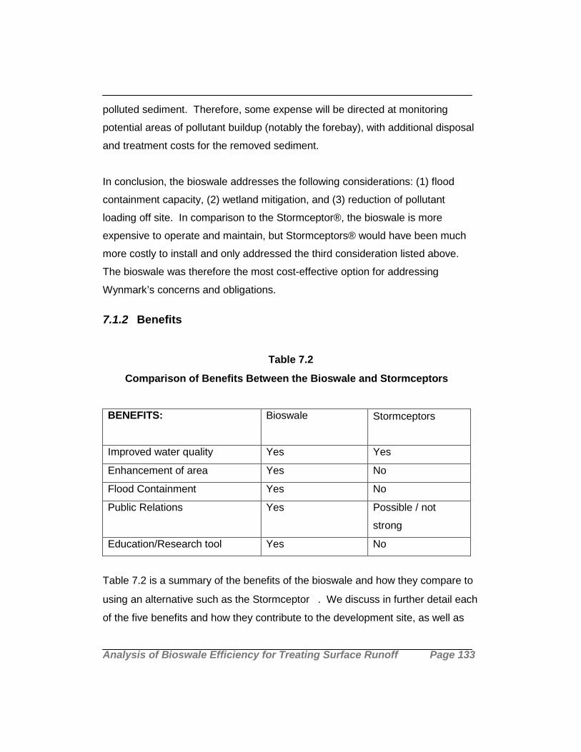
Analysis of Bioswale Efficiency for Treating Surface Runoff Page 133
polluted sediment. Therefore, some expense will be directed at monitoring
potential areas of pollutant buildup (notably the forebay), with additional disposal
and treatment costs for the removed sediment.
In conclusion, the bioswale addresses the following considerations: (1) flood
containment capacity, (2) wetland mitigation, and (3) reduction of pollutant
loading off site. In comparison to the Stormceptor®, the bioswale is more
expensive to operate and maintain, but Stormceptors® would have been much
more costly to install and only addressed the third consideration listed above.
The bioswale was therefore the most cost-effective option for addressing
Wynmark’s concerns and obligations.
7.1.2 Benefits
Table 7.2
Comparison of Benefits Between the Bioswale and Stormceptors
BENEFITS: Bioswale Stormceptors
Improved water quality Yes Yes
Enhancement of area Yes No
Flood Containment Yes No
Public Relations Yes Possible / not
strong
Education/Research tool Yes No
Table 7.2 is a summary of the benefits of the bioswale and how they compare to
using an alternative such as the Stormceptor . We discuss in further detail each
of the five benefits and how they contribute to the development site, as well as

Analysis of Bioswale Efficiency for Treating Surface Runoff Page 134
the practicality of using such water treatment systems in Santa Barbara County
and elsewhere.
Improved water quality refers to decreasing pollutant loading from the site. If
improved water quality were the only concern, there are several options to treat
surface runoff. In this case, the use of Fossil Filters® would be sufficient and the
additional expense of a bioswale would not be contemplated. Both systems trap
a portion of the pollutants that are generated in the Camino Real watershed, thus
improving the quality of water exiting the site. Modeling results indicated that the
bioswale’s TSS removal efficiency decreases as rain event size increases (Table
4.8). The Stormceptor® also provides decreasing TSS removal efficiency as flow
rate to the unit increases (Stormceptor® Corporation, 1996), but high rates of
removal efficiency are only true for a small treatment area (approximately 5
acres) for each unit.
Examination of the remaining benefits reveals that the bioswale is clearly
preferable to the Stormceptor . The bioswale provides flood storage capacity for
a two-year storm event, while the Stormceptor® provides no additional storage
capacity. After several years the plants in the bioswale will be established and
the bioswale will be an attractive open area, which contributes positively to the
community. Stormceptors® are underground and provide no additional visual
enhancement to a developed area. If the bioswale had not been installed this
area would have become an extension of the parking lots. The bioswale can
also serve as an education and research tool. Wynmark plans to install
informational signs near the bioswale and natural area to educate the public
about why they are there and how they function. The bioswale at Camino Real
also provides several additional areas for potential research. Sediment re-
suspension and vegetative pollutant uptake are two processes that were not
extensively evaluated during the course of this project. Both processes are

Analysis of Bioswale Efficiency for Treating Surface Runoff Page 135
interesting and useful research areas because they relate to long-term questions
about successful functioning of the bioswale.
Finally, the bioswale has a greater potential to improve public relations than an
unseen underground treatment device such as the Stormceptor®. In recent
months citizens of Santa Barbara County have voiced concerns about polluted
runoff in creeks and the resultant beach closures. Establishment of local
programs such as Project Clean Water and Save Our Shoreline represent the
county government’s response to citizen demand for action. The county is also
federally required to address pollution in urban runoff under the requirements of
the National Pollutant Discharge Elimination System (NPDES).
Implementation of Phase II of NPDES began in Santa Barbara County March 1,
1999, with stormwater discharge permits likely being required beginning May 31,
2002 (City of Monterey, et al., 1998). While Phase II does not specifically
require discharge permits for existing commercial facilities, Santa Barbara
County may enact more stringent requirements if it develops its own urban runoff
program. Wynmark knew about the upcoming regulations, and their installment of
an advanced water treatment system that meets NPDES specifications reduces
future uncertainty. Therefore, the bioswale becomes a benefit to the developer
by avoiding potential problems such as expensive retrofitting of storm sewer
systems. The following section provides more detailed information about the
NPDES permit process and how it relates to urban runoff programs. An urban
runoff program for Santa Barbara County is a natural extension of the NPDES
permit application process, and will contain guidelines that regulate future
development practices.

Analysis of Bioswale Efficiency for Treating Surface Runoff Page 136
7.2 Regulatory Framework for Stormwater Management
The U.S. Congress amended the federal Clean Water Act (CWA) in 1987 to
require stormwater discharge permits under the U.S. EPAs National Pollutant
Discharge Elimination System (NPDES). This was known as Phase I of NPDES,
and since 1990 it has required permits for stormwater discharges from
municipalities with populations over 100,000, specific industrial activities, and
construction activities disturbing 5 or more acres of land. Phase I of NPDES was
intended only to minimize combined sewer overflows (CSOs). CSO technically
refers to an overflow event from combined stormwater and sewage discharge,
but does not assume that sewage systems frequently overflow into storm drain
systems. Polluted discharge from stormwater drainage is considered enough of
a problem by itself to warrant the establishment of urban runoff programs (City of
Monterey, et al., 1998). In 1993 the EPA published an expansion of the original
policy under Phase II of NPDES. Phase II of NPDES expands the original
program to include all municipalities within designated urbanized areas, and
small municipalities outside of urbanized areas with a population of at least
10,000 and/or a population density of at least 1,000 persons per square mile
(City of Monterey, et al., 1998). Phase II also includes construction sites that
disturb between 1 and 5 acres.
The expansion of NPDES under Phase II include goals for much stricter
regulation of CSOs, including a wet weather management plan for CSOs such
that specific water quality standards would be achieved. Phase II of NPDES is
considered a landmark policy in two respects. First, Phase II resulted from a joint
collaboration of U.S. EPA, environmental groups, and municipalities. Second,
the policy contains a presumptive clause with respect to meeting water quality
standards (Roesner and Traina, 1994). The presumptive approach is the major
tool for evaluation of alternatives to be used for a long-term CSO program, as
outlined in Roesner and Traina (1994). If any of the following criteria are met by

Analysis of Bioswale Efficiency for Treating Surface Runoff Page 137
a CSO control plan, the program is “presumed” to provide an adequate level of
control to meet CWA requirements. 1) No more than four overflow events per
year for urban areas (5 for rural areas) are permitted, although the permitting
authority may allow up to two additional overflow events per year. 2) On a
system-wide annual average annual basis, no less than 85% by volume of
combined sewage collected in the combined sewer system during rainfall events
will be captured for treatment. 3) For the volume of collected sewage, the mass
of pollutants identified as causing water quality impairment will be eliminated or
reduced.
Phase II of NPDES was implemented March 1 of 1999. Santa Barbara County
and the Cities of Lompoc, Santa Maria, Santa Barbara, and Carpinteria are
included in the list of counties and incorporated places automatically designated
under Phase II, according to the 1990 Census of Population and Housing.
Phase II permits are anticipated to be required as of May 31, 2002 (City of
Monterey, et al., 1998). At this point it has not been determined whether the
entire County of Santa Barbara will apply for a joint permit, or if cities such as
Lompoc and Santa Maria will apply for permits individually (Aston, personal
communication). A natural progression of the permit application process is the
establishment of a countywide urban runoff program. Such a program could be
modeled after City of Monterey, et al. (1998), or other areas in California such as
Ventura County, San Diego County, and the City of Los Angeles that have
already established stormwater management programs.
The establishment of an urban runoff program for Santa Barbara County would
serve to formalize stormwater management practices for the County, which
currently occur on a more informal basis. The implementation of an urban runoff
program involves the following six main areas that are considered mandatory for
meeting NPDES requirements: 1) Public involvement and participation 2) Public
education and outreach 3) Illicit connection and discharge detection/elimination
4) Municipal operations control 5) Construction site control and 6) New

Analysis of Bioswale Efficiency for Treating Surface Runoff Page 138
development/redevelopment control. Phase II of NPDES does not specifically
address commercial, industrial, or residential pollutant sources that already exist.
Industrial sources are considered to be addressed under existing Phase I
regulations (the requirement to control all pollutants under a general permit).
Commercial and residential sources of pollution can be addressed through
education and outreach efforts. The Model Urban Runoff Program guidelines
(City of Monterey, et al., 1998) do include commercial facilities control and
industrial facilities control, however, as optional portions of urban runoff
programs.
The installation of the bioswale at the Camino Real development can be
considered an anticipation of potential future regulations governing the operation
of commercial facilities under a future Santa Barbara County Stormwater
Management Plan. Construction at Camino Real will be complete before Phase
II is effective and the development would be considered existing (and therefore
not specifically regulated under Phase II of NPDES), but the potential exists that
Santa Barbara County would incorporate the “optional” commercial and industrial
facilities controls as a required part of their plan. This could impact existing
developments through the requirement of stormwater system retrofitting to
achieve runoff quality goals.

Analysis of Bioswale Efficiency for Treating Surface Runoff Page 139
8.0 Design Assessment
The bioswale design chosen for the Camino Real Site is one of many possible
designs. Since the bioswale is not expected to be fully functional within the time
frame of this report, a full analysis of the success of this specific design at this
specific site will not be possible. Comparing the bioswale design with other
surface runoff treatment designs, however, provides an initial prediction of the
success of the bioswale.
8.1 Existing Bioswale Design Standards
Although bioswales are rare in Southern California, they have been used for
many years in the Pacific Northwest. King County, Washington has recently
updated its Surface Water Design Manual, giving detailed design
recommendations for bioswales that reflect their long-term experience with a
variety of designs. This section compares the bioswale at the Camino Real Site
with King County’s requirements.
The bioswale at Camino Real corresponds most closely to what the King County
Surface Water Design Manual (KCSWDM) refers to as a wet biofiltration swale.
A wet biofiltration swale is a variation of a basic biofiltration swale
for use when the longitudinal slope is slight, water tables are high,
or continuous base flow is likely to result in saturated soil
conditions. Where saturation exceeds about 2 weeks, typical
grasses will die. Thus, vegetation specifically adapted to
saturated soil conditions is needed. (KCSWDM p. 6-50)

Analysis of Bioswale Efficiency for Treating Surface Runoff Page 140
The bioswale at Camino Real closely matches this definition because the
longitudinal slope of the site is slight, and daily low flows from irrigation and
pavement washdown are likely to result in saturated soil conditions and a
persistent “micropool” at the southern end of the bioswale.
The KCSWD Manual (1997) provides a series of calculations for designing a
bioswale that is expected to meet the Basic Water Quality goal of 80% TSS
removal. King County has not frequently used bioswales to treat runoff from
commercial sites of this size, but the design calculations from the Surface Water
Design Manual would still apply to a large site (Kulzer, personal communication).
Table 8.1 shows the dimensions of the backbay of the bioswale at Camino Real
and recommended dimensions based on the calculations outlined in the KCSWD
Manual. The Manual calculations are based on a water quality design flow that is
sixty- percent of the two year, 24 hour rain event. This water quality design flow
is then used to estimate the size of the wet biofiltration swale that is expected to
reduce TSS by 80 percent. As with the Camino Real bioswale, King County
recommendations are based on the expectation that swales will deal with more
frequent low intensity rains and daily low flows from irrigation and washdowns.
Table 8.1Dimensions of the Bioswale at Camino Real and King County
Recommendations
Bioswale at Camino Real(Backbay)
KCSWDM(Calculated)
Treatment Area (sq. ft.) 21750 53150Length (ft.) 290 516Width (ft.) 75 103Side Slopes (H:V) 2:1 Not steeper than
2:1Design Flow Velocity (fps) 0.25 Less than 1.0

Analysis of Bioswale Efficiency for Treating Surface Runoff Page 141
The King County Surface Water Design Manual specifies a variety of design
parameters including: flow velocity, aspect ratio of the swale, slope stabilization,
use of riprap, planting designs, bypasses, and detention times. The bioswale at
Camino Real is compliant with the KCSWD Manual, excluding the treatment
area. Although the bioswale is smaller than the King County recommendations,
placing undersized biofiltration swales in available space is allowed (KCSWDM,
1997). The use of a forebay is known to reduce the backbay size necessary to
meet treatment goals. Since the forebay is not included in the calculations, the
effective treatment area of the Bioswale at Camino Real is somewhat larger than
the 21750 sq. ft. calculated. The King County Surface Water Design Manual
does not address the use of a forebay in calculations, but would likely require a
larger backbay regardless. An example bioswale from the KCSWD Manual is
included in Figure 8.1.
We conclude that though the bioswale is smaller than the ideal suggested by
KCSWDM calculations, the more than doubling of area necessary to meet
KCSWDM standards is not an efficient use of the area. As shown in Table 4.10,
increasing the bioswale by 2.4 times it’s present size (without a forebay) results
in the removal of 54% of Total Suspended Solids (TSS) during a 0.15 in/hr storm,
and a removal of 30% TSS during a 2-year storm. Similarly, Table 4.9 shows the
effectiveness of the bioswale in TSS removal during the same two types of storm
events, with no increase in area. Removal rates are 46% TSS for the 0.15 in/hr
storm and 25% for the 2-year storm, based on expected settling velocities in the
bioswale when vegetation is fully established.

Analysis of Bioswale Efficiency for Treating Surface Runoff Page 142
Figure 8.1Example Bioswale from the King County Surface Water Design Manual
������
berm or baffle at design WS or submerged 1’ below design W.S. Extend berm across entirewetpool width.
plantings required on cut slopes for lake protection facilities
emergency spillway per detention facility requirements
FIRST WETPOOL CELL25% to 35% of wetpool volume,
excluding access ramp
access ramp to bottom of firstwetpool cell (7H: 1V) (see text)
SECOND WETPOOL CELL
emergency overflow WS
overflow WS wetpoolwidth
PLAN VIEWNTS
inlet pipe & catch basin perdetention facility requirements
outlet erosion control & energy dissipation per detention facility requirements
manhole & outlet pipe pie sized to pass peak flow perconveyance requirements
A
A
B
B
WQ design WS
berm top width 5’ min. (if earthen)
access road to outlet structure
access road to inlet structure
New Design ManualFigure 6.4.1.B WetpondRevised 4-15-97, mdev
NOTE: Berm not required for ponds with length to width ratio ≥ 4:1 or if volume less than 4000 c.f.
(Source: King County Surface Water Design Manual, 1997)

Analysis of Bioswale Efficiency for Treating Surface Runoff Page 143
9.0 ConclusionsIn the introduction, we listed the three questions the group intended to answer:
• To what extent does the bioswale improve water quality?
• What is the total impact of the bioswale in the Devereux Creek Watershed
• Given other available options, is the bioswale a cost-effective water treatment
method?
In this section, based on our research, sampling, and modeling efforts, we
answer the three main questions. Since construction is not completed and
vegetation is not fully established in the bioswale, many of our results are
preliminary. Conclusions are based on limited field data and are necessarily
cautious since only a few storm events were measured.
9.1 To what extent does the bioswale improve waterquality?
Chemical sampling results indicated small decreases in concentration between
the bioswale inlet and outlet for most parameters (Table 5.3). Statistical analysis
revealed that the decreases are not statistically significant. We cannot conclude
at this time that any observed differences in concentration are due to bioswale
processes (settling of suspended sediment and plant uptake) rather than inherent
spatial and temporal variability in the stormwater samples. Some concentrations
increased slightly between the bioswale inlet and outlet, and are again
interpreted to be due to individual sample variability. In the case of increased
total suspended solids, the observation of bare soil with gullies next to the
bioswale outlet sampling location leads to the hypothesis that increases in TSS
at the bioswale outlet are a temporary function of the currently incomplete
vegetation growth and erosion from the banks in the bioswale (Figure 5.2).

Analysis of Bioswale Efficiency for Treating Surface Runoff Page 144
Modeling results, however, predict a strong role for the bioswale in water quality
improvement. Most modeling scenarios were conducted without the orifice plate
in place, since removal of the orifice plate is recommended, and its removal
should be a simple operation. Comparison of model runs with and without the
orifice plate in place show improved bioswale efficiency in reducing total TSS
loads leaving the study site when the orifice plate is removed. Modeling
conclusions are therefore based on simulations conducted with the orifice plate
removed within the model.
Modeling results indicate that in its current unfinished state, the bioswale is
effective in removing TSS from the water it receives for very small storms or
other low flow runoff from irrigation or washdown. For a 2 hour storm with 0.03
in/hr intensity, the modeled bioswale removes 77% of the TSS it receives. This
effectiveness drops sharply as storm intensity increases. For a 2 hour storm with
0.15 in/hr intensity, the modeled bioswale removes 26% of the TSS it receives.
When the bioswale's soil and vegetation become established, simulations show
the bioswale's effectiveness will improve for all storm events. In addition, the
drop in effectiveness due to increased storm size is not expected to be as
dramatic after vegetation becomes established.
The model simulations performed show that bioswales have the potential to
significantly reduce TSS and pollutant loads leaving a developed site, particularly
for small storm events. Developed areas could benefit from their application,
especially in areas with no other means of runoff control. The effectiveness of
bioswales is somewhat dependent upon their capacity to receive and retain
flows, however. Bioswales are limited in the amount of water they can process.
Within the frame of runoff from a large area, their impact may be relatively small,
depending upon the size of the bioswale. In addition, other means for reducing
TSS and pollutants in stormwater runoff may already be in place.

Analysis of Bioswale Efficiency for Treating Surface Runoff Page 145
At the study site, modeling indicates that the natural area, because of its larger
area, lower gradient, and thicker vegetation, is a more effective mechanism for
the removal of TSS and other pollutants than the bioswale in its current
unvegetated state. This holds true even when the model is calibrated to simulate
the bioswale's future functioning. The model also indicates that the natural area
is almost as effective at removing TSS and other pollutants by itself as when
coupled with the bioswale. Model simulation show that the bioswale improves
the overall removal of TSS by about 4-19% of the total load generated by the
site. If the natural area is a habitat that needs protection from stormwater runoff,
however, the bioswale will significantly reduce the loading to the natural area.
Presence of a forebay appears to have an impact on the effectiveness of a
bioswale. During model simulations, the area of the forebay of the bioswale was
increased, while the overall area of the bioswale was not changed. Results from
these simulations indicate that a larger forebay improves bioswale effectiveness,
especially for smaller storms. Further modeling showed that a bioswale without a
forebay, but of a larger size, is not as effective for small storms as the bioswale
design implemented at Camino Real. This is significant, since bioswales are
generally designed to be effective during the low flow conditions of first flushes or
small storms.
9.2 What is the total impact of the bioswale in theDevereux Creek Watershed?
The bioswale at Camino Real processes approximately 3% of the total runoff
within Devereux Creek Watershed; the remainder of urban land uses--58% of the
watershed--lacks this level of stormwater runoff quality protection (Figure
9.1,9.2). In order to preserve the wetland and estuarine habitats of the Devereux

Analysis of Bioswale Efficiency for Treating Surface Runoff Page 146
Slough, action must be taken throughout the watershed to prevent the increased
sedimentation and water quality problems associated with urban storm water
runoff (see Section 5.1) from reaching the Slough. The bioswale at Camino Real
is an important first step in addressing the preservation of the Slough. Since
vegetation establishment is not yet complete, the final evaluation of the success
of the bioswale is outside the scope of this report. However, the goals of the
bioswale, which include keeping sediment and contaminants on site, are exactly
what is required to preserve the wetland and estuarine habitats. Carey, et al.,
(1998) noted that wetland protection requires coherent action and consistent
planning on a watershed scale. Mitigation to improve stormwater runoff quality
should be included for the 11% of the watershed that is zoned for future
development, but the maintenance of the long-term health of the Devereux
Slough ecosystem will also require stormwater pollution prevention at existing
urban land uses within the watershed.
Figure 9.1Existing Land Use in the Devereux Creek Watershed
A variety of BMPs are available to prevent or reduce stormwater pollution on
existing or future urban land developments. Once the vegetation has been
established and monitoring of the bioswale reveals that it achieves its goals of
improving stormwater runoff quality, then bioswales should be seriously
58%
11%
31%Urban
UrbanUndevelopedNon-Urban

Analysis of Bioswale Efficiency for Treating Surface Runoff Page 147
considered as a BMP for stormwater pollution prevention at future development
sites in the Devereux Creek Watershed. Considerations of economic feasibility
will also be a dominant factor in deciding on a BMP. Bioswales are unlikely to be
deployed at existing urban development within the watershed because 1)
bioswales require land which is expensive and which is frequently unavailable at
existing developments and 2) there is no legal pressure for existing sites to
improve their stormwater runoff quality.

Analysis of Bioswale Efficiency for Treating Surface Runoff Page 148

Analysis of Bioswale Efficiency for Treating Surface Runoff Page 149
9.3 Given other available options, is the bioswale a cost-effective water treatment method?
If improved water quality were the only concern, there are several options to treat
surface runoff. The use of Fossil Filters® or Stormceptors® would be sufficient
and the additional expense of a bioswale would not be contemplated. However,
the bioswale addresses the following considerations: (1) flood containment
capacity, (2) wetland mitigation, and (3) reduction of pollutant loading off site.
The bioswale was therefore the most cost-effective option for addressing
Wynmark’s concerns and obligations.
The bioswale provides flood storage capacity by acting as a detention basin,
while the Stormceptor® and Fossil Filter® options provide no additional storage
capacity. Maximum storage for the bioswale occurs during a 2-year flood event,
however the combination of bioswale, natural area and playfields contains a 100-
year flood event. The bioswale was placed to take advantage of a remnant
stream channel and thus avoided costly floodwater detention construction
elsewhere on the development site.
A minimum replacement ratio of 2:1 was required by the EIR for the loss of
wetlands existing on the site before construction. From the beginning of the
project development, the natural area was to remain and be enhanced to
maintain open space, but off-site habitat restoration within the Devereux Creek
watershed would still have been required. The installation of the bioswale, in
conjunction with the natural area, accounted for full wetland mitigation according
to the Army Corps of Engineers. An option such as the bioswale is cost-effective
when compared to off-site restorations that are more expensive and more difficult
to implement and monitor. Again, neither the Stormceptor® nor Fossil Filter®
options provided mitigation for wetland loss.

Analysis of Bioswale Efficiency for Treating Surface Runoff Page 150

Analysis of Bioswale Efficiency for Treating Surface Runoff Page 151
10.0 Report Recommendations
Based on the conclusions of our report, we make the following
recommendations:
• Expand Bioswale Management Plan
• Review Performance of the Bioswale
• Maintain Oil and Grease Devices
• Remove Orifice Plate
• Modify Energy Dissipator
10.1 Expand Bioswale Management Plan
The expansion of the Bioswale Management Plan will facilitate management of
the bioswale and help to ensure efficiency and effectiveness of bioswale
performance. This plan is necessary because of the variety and complexity of
tasks associated with bioswale inspection, maintenance, testing, and
performance review.
In order to achieve the stated goals as well as justify the costs associated with
the bioswale, effective and efficient performance is vital. To ensure that the
bioswale fulfills these goals correctly and continues to perform up to these
standards, inspection, maintenance, and performance monitoring are essential
post-construction activities. These activities are equal in importance to the
planning, design, and construction of the bioswale. Failure to meet these
responsibilities would diminish the performance of the bioswale, and could
conceivably create new health and safety issues exceeding those which the
bioswale was intended to prevent. Included below are brief descriptions of

Analysis of Bioswale Efficiency for Treating Surface Runoff Page 152
elements intended to supplement and reinforce the existing Bioswale
Management Plan. This section provides brief descriptions of elements intended
to supplement and reinforce the existing Bioswale Management Plan.
10.1.1 Identify Team Members
Identify individuals within the facility organization to be members of a Bioswale
Management Team. Establish responsibility for developing the plan and assisting
in its implementation, maintenance, and revision. The responsibilities of each
team member must be clearly identified.
10.1.2 Assess Sources of Pollutants
Provide a description of potential sources that may be reasonably expected to
add significant amounts of pollutants to storm water discharges. Additionally
provide a description of pollutants which may be spilled and result in the
discharge of pollutants during dry weather. Important spatial differences in
contaminant loading are to be expected due to the variety of land uses within the
159 acres the bioswale serves. Additionally, equipment and areas that have the
potential for failures or spills must be identified.
10.1.3 Source Reduction
The life expectancy of the bioswale, like all filters, is strongly determined by the
quantity and type of pollutants that it is required to filter. Direct reduction of
pollutant loading at the identified potential sources of contamination will greatly
benefit water quality and bioswale longevity. Examples of contaminant source

Analysis of Bioswale Efficiency for Treating Surface Runoff Page 153
reduction include: frequent street and parking lot sweeping, avoidance of
excessive fertilizer and pesticide use, and trained onsite personnel available for
spill containment and cleanup.
10.1.4 Inspection
The explicit and official inclusion of regular bioswale inspection in the Bioswale
Management Plan is vital. Regular inspection allows repairs to be performed
promptly without the need for major remedial or emergency action. In view of the
complex nature of the bioswale and the wide range of technical aspects, the
need for competent inspectors is obvious. A team of inspectors may be
necessary to adequately review the geotechnical, environmental performance,
structural, hydraulic, and biological aspects of the bioswale. Designated
personnel should conduct inspections and report to the Pollution Prevention
Team member responsible for inspections. Examples of inspection tasks include:
• Creation of inspection sheets and their use by inspection personnel during
inspections.
• Inspection of storm water inlets, storm sewer pipes, and other storm water
control features and clearing of debris after each major storm event and at a
minimum of once a month. Record current physical condition of storm water
control features.
• Inspection of natural area and clearing of debris after each major storm event
and at a minimum of once a month. Record and photograph physical
conditions (erosion, sedimentation, and structural integrity), biotic conditions
(plant health, plant abundance and animals present), and water levels.
• Conduct comprehensive site inspection semi-annually to update pollutant
sources and source reduction opportunities.

Analysis of Bioswale Efficiency for Treating Surface Runoff Page 154
10.1.5 Maintenance
The essence of any site management plan is the regular, consistent performance
of the actual maintenance tasks that the Bioswale Management Plan has
identified, planned, and scheduled, and for which staff, equipment, and funding
have been provided. The competent and consistent performance of these routine
tasks is the single greatest factor in determining the overall success of the overall
Bioswale Management Plan. These routine tasks may include watering,
trimming, trash and debris removal, soil fertilization, and sediment removal.
Experience has shown that the regular, frequent (monthly or less) performance of
these tasks often requires less overall time and effort on an annual basis than if
the tasks are performed only a few times a year.
In addition, modeling results indicate that sedimentation within the forebay of the
bioswale will begin to clog the forebay drainage pipes after approximately 4-5
years of average rainfall. The pipes are expected to be covered with sediment
after approximately 8-10 years. We therefore recommend that sedimentation
within the forebay be monitored, and a plan to excavate excess sedimentation
every 4 years be implemented.
A list of management issues and response actions is presented in Table 10.1.
Table 10.1Management Issues and Actions
MaintenanceComponent
Defect Conditions WhenMaintenanceIs Needed
ResultsExpected WhenMaintenance IsPerformed
General Trash & Debris Any trash and debriswhich exceed 1 cubic footper 1,000 square feet(this is about equal to theamount of trash it would
Trash anddebris clearedfrom site.

Analysis of Bioswale Efficiency for Treating Surface Runoff Page 155
take to fill up onestandard size officegarbage can). In general,there should be no visualevidence of dumping.
PoisonousVegetation
Any poisonous ornuisance vegetationwhich may constitute ahazard to MaintenancePersonnel or the public.
No danger ofpoisonousvegetationwhereMaintenancepersonnel or thepublic mightnormally be.
Pollution Oil, gasoline, or othercontaminants of onegallon or more or anyamount found that could:1) cause damage toplant, animal, or marinelife; 2) constitute a firehazard; or 3) be flusheddownstream during rainstorms.
Nocontaminantspresent otherthan a surfacefilm.
Drought Extended droughtthreatens vegetationsurvival.
Irrigate plants toensure survival.
Rodent Holes Any evidence of rodent orany evidence of waterpiping through dam orberm via rodent holes.
Rodentsdestroyed anddam or bermrepaired.
Insects When insects such aswasps and hornetsinterfere withmaintenance activities.
Insectsdestroyed orremoved fromsite.
Weeds Weeds threatenestablishment of nativevegetation or, afterestablishment, grow inthe Bioswale.
WeedsRemoved
Tree Growth Tree growth does notallow maintenanceaccess or interferes withmaintenance activity (i.e.,slope mowing, siltremoval, or equipmentmovements). If trees arenot interfering withaccess, leave treesalone.
Trees do nothindermaintenanceactivities.

Analysis of Bioswale Efficiency for Treating Surface Runoff Page 156
Side Slopesof Bioswale
Erosion Eroded damage over 2inches deep where causeof damage is still presentor where there ispotential for continuederosion.
Slopes shouldbe stabilized byusingappropriateerosion controlmeasure(s);e.g.,reinforcement,wood chips.
Storage Area Sediment Accumulated sedimentthat exceeds 10% of thedesigned pond depth.
Sedimentcleaned out todesigned pondshape anddepth; pondreseeded ifnecessary tocontrol erosion.
Spillway Rock Missing Only one layer of rockexists above native soil inarea five square feet orlarger, or any exposure ofnative soil at the top ofout flow path of spillway.Rip-rap on inside slopesneed not be replaced.
Replace rocksto designstandards.
Pipes Sediment &Debris
Accumulated sedimentthat exceeds 20% of thediameter of the pipe.
Pipe cleaned ofall sediment anddebris.
Vegetation Vegetation that reducesfree movement of waterthrough pipes.
All vegetationremoved sowater flowsfreely throughpipes.(AfterKCSWDM,1997)
Despite the best efforts of any management program, emergency maintenance
measures may be necessary at the bioswale from time to time for a variety of
causes, ranging from excessive rainfall to vandalism. As a result, the successful
inspection and maintenance program must be ready to respond to this need in a
timely and comprehensive manner. To do so, it is best to plan ahead for
emergencies by developing an emergency response plan that identifies potential

Analysis of Bioswale Efficiency for Treating Surface Runoff Page 157
emergency problems and ways to address them. This may include the
preparation of a list of typical repair materials, which then can be either
stockpiled in house or quickly acquired through designated suppliers. The plan
may also identify individuals and organizations that can provide technical input or
services on short notice to assist in the emergency repair effort. Finally, a
designated number of staff personnel should be available on a 24-hour basis to
respond to maintenance emergencies.
10.2 Review Performance of the Bioswale
Rainfall-runoff processes are inherently complex and it can be difficult to
determine how well water quality goals are being met, regardless of the
proficiency of BMP design, construction, and maintenance efforts. For this
reason, performance monitoring of the bioswale is essential. Evaluation of
bioswale performance through field monitoring, sampling, and careful analysis of
field data will provide the information necessary to address several concerns.
One major concern is the potential impact of polluted runoff on Devereux Slough.
Even though the total amount of runoff the bioswale will treat is small relative to
the total amount generated within the Devereux Creek watershed, the bioswale
filters the most contaminated portion and contributes positively to the incremental
reduction of pollutants that reach the Slough.
Formal performance review of the bioswale will facilitate the evaluation of the
bioswale as an cost-effective solution to stormwater detention, water quality
improvement, and wetland habitat replacement. This information will allow
developers and regulators to assess the applicability of bioswales in future
developments. Furthermore, the chemical sampling recommended for
performance review will help to characterize the gradual accumulation of

Analysis of Bioswale Efficiency for Treating Surface Runoff Page 158
contaminated sediment in the bioswale and provide an early warning of possible
ecological or disposal hazards associated with contaminated sediments.
In addition, bioswale performance monitoring can also be seen as a way to help
ensure overall program credibility and achieve stronger community acceptance.
In recent years, much attention has focused on the need to expand traditional
stormwater management programs beyond structural measures, such as a dry
detention pond, to also include nonstructural measures in order to achieve more
comprehensive results. With the real data obtained through bioswale
performance monitoring, it will be easier to convince the community of both the
need for and the promise of stormwater management. Finally, bioswale
performance monitoring will help to more closely monitor progress and more
quickly identify program problems and shortcomings. This will help to develop
and implement program modifications and improvements that enhance
community acceptance. Specific recommendations for water and sediment
sampling are outlined in the following section.
10.2.1 Minimum Chemical Analysis Recommendations for BothSediment and Water
Table 10.2 presents minimum recommendations for sample analysis. The
primary source of this information was the Guidance for Monitoring the
Effectiveness of Stormwater Treatment BMPs (EOA, 1996), and is reinforced in
other documents such as Monterey, et al., (1998). The list includes the four main
areas of pollutant concern (sediment, nutrients, metals, and hydrocarbons) that
were analyzed during the group project. Addition of particle size distribution and
total dissolved solids is recommended to improve understanding about pollutant
partitioning and the fate of pollutants in the bioswale. Field measurements are
recommended because they are an inexpensive source of information about

Analysis of Bioswale Efficiency for Treating Surface Runoff Page 159
changes in water quality between the bioswale inlet and outlet, and about water
quality exiting the site at the natural area outlet.
Table 10.2Recommended Parameters for Assessing the Effectiveness of BMPs
Parameter Media Practical Quantitation LimitGeneral, Physical, andInorganic Non-MetalsTSS Water 5.0 ppmTDS " 5.0 ppmHardness " 5.0 ppmParticle Size Distribution Water and Sediment NANutrientsNO3 + NO2 (as N) Water 0.1 ppmNH3 (as N) " 1 ppmTotal Phosphorus (as P) " 0.5 ppmOrthophosphate (as P) " 0.5 ppmTotal and Dissolved MetalsCopper Water and Sediment 0.5 ppmLead " 1.0 ppmZinc " 1.0 ppmAntimony Sediment 5.0 ppmArsenic " 5.0 ppmBarium " 0.5 ppmBeryllium " 0.5 ppmCadmium " 1.0 ppmChromium " 1.0 ppmCobalt " 1.0 ppmMercury " 0.1 ppmMolybdenum " 1.0 ppmNickel " 1.0 ppmSelenium " 5.0 ppmSilver " 1.0 ppmThallium " 5.0 ppmVanadium " 1.0 ppmOrganic ConstituentsTotal Petroleum Hydrocarbons Water and Sediment 1.0 ppmField MeasurementspH Water NATemperature " NAConductivity " NA
NA = Not ApplicableItalicized metals are not required, but along with Copper, Lead, and Zinc comprise the CAM-17list of metals regulated by the State of California.Source: Modified from EOA, (1996).

Analysis of Bioswale Efficiency for Treating Surface Runoff Page 160
10.2.2 Chemical Sampling Considerations
The purpose of performing chemical sampling and data analysis is to aid in the
review of the performance of the bioswale. The minimum analysis
recommendations for sediment and water described above will allow bioswale
managers to track and evaluate known and existing bioswale performance
concerns. Unfortunately, not all possible bioswale performance issues or the
relative importance of these performance issues can be known at this time. If
new performance issues arise, chemical sampling and data analysis should be
tailored to address these new performance issues. This section provides a
general background in chemical sampling and analysis, as well as information on
how the minimum analysis recommendations were selected.
10.2.2.1 Assessment of Sediment Contamination
The bioswale is designed to filter sediment, nutrients, and contaminants found in
urban stormwater runoff. Although some pollutants are expected to degrade,
many will accumulate over time, leading to contaminated sediments within the
bioswale. Many contaminants the bioswale is expected to filter can be
hazardous at high concentrations. In King County, Washington, sediments
excavated from biofiltration swales are frequently hazardous and require
treatment before disposal (Kulzer, personal communication). Accurate
prediction of contaminant loading rates to the bioswale is limited by several
factors, including the spatial and temporal variability of both the types and
quantity of pollutants that will loaded on the site, the stochastic nature of the
storms that transport pollutants, and uncertainty regarding the fates of
contaminants within the bioswale (U.S. EPA ,1992). Given these factors, the
long term monitoring of sediments is important to performance analysis of the
bioswale, and provides information useful for avoiding hazards associated with

Analysis of Bioswale Efficiency for Treating Surface Runoff Page 161
contaminated sediments. This section addresses sample design and collection
and chemical and physical analyses. We emphasize that a broad range of
information regarding sampling and analysis is presented in the following section,
and represents a comprehensive ideal for a monitoring program.
10.2.2.2 Sediment Sampling Design
The goals of sediment sampling in the bioswale are to determine current levels of
sediment contamination, and to track long-term changes in sediment
contamination. Continued sampling is necessary because 1) characterization of
contaminant loading from the fully built out site cannot be accurately predicted
from existing site conditions 2) if excavated sediment is contaminated, the nature
of the contamination will have to be characterized for proper disposal and 3) site
use and subsequent pollutant loading may change over time. For example,
changes in fuel and oil use may alter contaminant loading to parking lots.
Preliminary modeling results suggest that sediment loading could begin to clog
the pipes that convey flow to the backbay in as soon as four years. At minimum,
sediments should be analyzed in the forebay and backbay of the bioswale, as
well within the natural area, before any excavation of sediments.
As part of this project, pre-pollutant loading sediment samples were collected in
the forebay. Results of this sampling are available in Table 5.4. These data
provide the initial conditions necessary to track changes in sediment
contamination. Based on the results of this testing, we have made specific
recommendations for future sampling that is intended for reconnaissance and
simple tracking of sediment condition. More extensive sampling not outlined in
this document should be undertaken if hazardous concentrations of contaminants
are found in the sediments.
Analysis of Bioswale Efficiency for Treating Surface Runoff Page 162
10.2.2.3 Sediment Chemistry and Physical Analyses
The bioswale group did not perform extensive sampling and analysis of
sediment. The main focus of the project was hydrology and water quality, but a
logical extension of water quality sampling is investigation of sediment
contaminant loading over time. Included below is a comprehensive list of
parameters that are of general concern for sediments. This list does not
necessarily represent the actual list of parameters that would be routinely tested
at the Camino Real bioswale. The need for trained sampling personnel and the
high expense of certain analyses will eliminate certain tests from routine analysis.
• Particle or grain size of sediment is a physical parameter that determines the
distribution of particles. Size is important because finer grained sediments
tend to bind contaminants more than coarse sediments do.
• Total organic carbon (TOC) is an important indicator of bioavailability for
nonionic hydrophobic organic pollutants.
• Acid volatile sulfides (AVS) can indicate the presence of toxic sediment-
related metals.
• Polyaromatic hydrocarbons (PAHs) are semivolatile organic pollutants,
several of which are potential carcinogens and are linked to tumors in fish.
• Polychlorinated biphenyls (PCBs) are highly toxic, chlorinated organic
compounds once used for numerous purposes, including as a dielectric fluid
in electrical transformers.
• Pesticides are synthetic compounds predominantly used in agriculture to
control crop-damaging insects. Pesticides are known to have acute and
chronic ecosystem impacts.
• Other semivolatiles, including acid/base neutral compounds (ABNs) such as
phenols, naphthenes, and toluenes.

Analysis of Bioswale Efficiency for Treating Surface Runoff Page 163
• Heavy metals are naturally occurring in the environment, but an excess of
metals can be an indication of anthropogenic contamination; heavy metals
can be toxic to benthic organisms.
(Source: Dennis-Flagler, 1995)
10.2.2.4 Water Quality Assessment
A major purpose in the establishment of a long term water quality monitoring
program for the Camino Real bioswale is to establish a local water quality data
set that can be used to evaluate the overall effectiveness of the bioswale in
improving stormwater runoff quality. Another contribution of the bioswale is
expected to be the absorption of concentrated pollutants in small volume
irrigation and pavement washdown events, which aids in the prevention of
contaminated runoff reaching Devereux Slough. Evaluation of water quality data
can lead to an overall assessment of the bioswale as a Management Practice,
and whether other bioswales would be a recommended management measure
for other development projects in the area. Information about water quality must
be combined with information about runoff volumes generated for a variety of
storm intensities, to evaluate the relative amount of stormwater runoff that the
bioswale is able to treat. The bioswale may not be able to handle large volumes
of runoff generated during large storm events, but is expected to be effective in
treating small rain events and small volumes of runoff generated during irrigation
and cleaning operations such as pavement washing.
10.2.2.5 Water Quality Sampling Design and Collection
Recommendations for water sampling design are the same as those outlined in
the description of chemical sampling performed for the group project. Refer to
Sections 5.1 and 5.2 for a review of information on pollutants that are of concern
in stormwater and sampling design recommendations. We emphasize the

Analysis of Bioswale Efficiency for Treating Surface Runoff Page 164
importance of collecting a series of samples and flow measurements at each
sample location for adequate establishment of Estimated Mean Concentration
(EMC) values. Attempting to sample the runoff generated at the very beginning
of each rain event is also emphasized. Information about first flush
concentrations is essential for long term evaluation of whether the bioswale is
treating the majority of this water, or whether a large proportion of polluted runoff
is being routed around the bioswale through the bypass pipe. The sampling
recommendations are a reflection of the efforts of a group of five people with a
yearlong focus on attempting to answer specific questions about the functioning
of the bioswale at Camino Real. Even with highly specific goals and close
monitoring of incoming storm events, it was difficult in practice to arrive at the
bioswale in time to capture first flush samples. We had five people locally
available for sample collection and this proved helpful, but in practice sample
collection is more likely to be the job of one or two people.
10.3 Maintain Oil and Grease Devices
Urban stormwater runoff carrying high concentrations of petroleum hydrocarbons
can significantly impact the filtration capacity of the bioswale. Careful
maintenance of the Fossil Filters® that have been installed will be necessary for
optimal bioswale performance, since the bioswale at Camino Real is receiving
petroleum hydrocarbon loading from two service stations, several high use roads,
intersections, and parking lots. A recommended goal of treatment is to have no
visible sheen for runoff leaving the facility, or to have less than 10 mg/L total
petroleum hydrocarbons (KCSWDM, 1997).

Analysis of Bioswale Efficiency for Treating Surface Runoff Page 165
10.4 Remove Orifice Plate
As mentioned previously in the hydrologic section, the orifice plate on the inlet to
the bioswale is diminishing the potential role of the bioswale. For a relatively
small design storm of 0.15 in/hr over two hours, the model indicated that the
bioswale's effectiveness in reducing the TSS loads leaving the site increased
with the removal of the orifice plate. This was due to the increase in the amount
of flow routed to the bioswale with the orifice plate removed. The percent of flow
from the site treated by the bioswale increased dramatically and the overall
removal of TSS by the bioswale and natural area was also increased without the
orifice plate in place.
10.5 Modify Energy Dissipator
The main impetus for placing an energy dissipator at the exit of a culvert pipe is
to reduce water velocity, thereby mitigating the effects of erosion. As mentioned
in the hydrologic section, when water exits the culvert pipe it is slowed down as it
enters the energy dissipator, but when it leaves the flow contracts through three
0.5-foot openings and the velocity leaving the energy dissipator increases
significantly. Some erosion has already been observed in the area where water
is discharged from the energy dissipator into the natural area. If the effects of
erosion become severe, the energy dissipator could be modified to slow down
the velocity at which water exits this device and thereby slow down the erosion
processes. To decrease its exiting velocity the three 0.5-foot openings could be
enlarged. The amount of flow leaving the energy dissipator would still be the
same, but the velocity at which this flow leaves could be decreased.
The energy dissipator may need to be cleaned out periodically because large
clumps of sediment have already been observed to be accumulating in it. The
main reason the energy dissipator is accumulating sediment is due to the fact it

Analysis of Bioswale Efficiency for Treating Surface Runoff Page 166
decreases the velocity of water as flow enters this device. This is further
enhanced by the energy dissipator’s ability to pond water as flow is only allowed
to leave through three 0.5-foot openings. In the future, the energy dissipator
should be monitored for sediment accumulation and possible erosion effects at
the entrance of the natural area.

Analysis of Bioswale Efficiency for Treating Surface Runoff Page 167
11.0 References
Anderson, R., and M. Rockel, 1991. Economic Valuation of Wetlands.Discussion Paper #065, American Petroleum Institute.
Anderson, T. and J. Coats, 1994. Bioremediation through RhizosphereTechnology. ACS Symposium Series #563.
Aston, D., 1999. Santa Barbara County Water Agency. Personal communicationregarding NPDES and county’s permit application requirements.
Baudo, R., Giesy, J. and H Muntau, 1990. Sediments: Chemistry and Toxicity ofIn-Place Pollutants. Lewis Publishers, Inc., Chelsea, MI. p. 265-293.
Bomkamp, T., 1999. Lead Biologist for the Camino Real Project Bioswale.Personal communication regarding selection of plants in the bioswale.
Brady, N.C. and Weil R.R., 1996. The Nature and Properties of Soils. PrenticeHall, Inc. New Jersey.
Breen, P.F., and B.S. Seymour, 1994. The Combination of a Flood-RetardingBasin and a Wetland to Manage the Impact of Urban Runoff. Water ScienceTechnology, 29(4)103-109.
Burken, J., Schnoor, G., and L. Jerald, 1996. Phytoremediation: Plant Uptake ofAtrazine and Role of Root Exudates. Journal of Environmental Engineering, 958-963.
Camp, Dresser & McKee Inc., et al., 1993. State of California Stormwater BestManagement Practices Handbooks, Volume 2: Industrial and Commercial.
Carey, J., de la Garza, M., Gebhard, T., Harris, J., and G. Heistand, 1998.Investigating the Cumulative Impacts of Land Use Change on Local WetlandsWatersheds. M.E.S.M. Thesis, University of Califonia, Santa Barbara.
Chow, V.T. 1959. Open-Channel Hydraulics. McGraw-Hill Book Company.
City of Monterey, City of Santa Cruz, California Coastal Commission, MontereyBay National Marine Sanctuary, Association of Monterey Bay Area Governments,Woodward-Clyde Consultants, and Central Coast Regional Water Quality ControlBoard, 1998. Model Urban Runoff Program: A How-To Guide for DevelopingUrban Runoff Programs for Small Municipalities.

Analysis of Bioswale Efficiency for Treating Surface Runoff Page 168
Clesceri, L. (ed.), 1989. Standard Methods for the Examination of Water andWastewater. Seventeenth Edition, APHA, AWWA, and WPCF.
Cunningham Design, Fuscoe Engineering, Inc., and K.O. Rogers, 1997. CaminoReal Natural Area and Bioswale Enhancement and Management Plan. Preparedfor Wynmark Company, Goleta, CA. 12 p.
Cunningham, S. D., and D. W. Ow, 1996. Promises and Prospects ofPhytoremediation. Plant Physiology, (110)715-719.
Daugherty, R., Franzini, J. and J. Finnemore, 1985. Fluid Mechanics withEngineering Applications. McGraw-Hill Publishing Company.
Davis, F.W., D. Theobald, R. Harrington, and A. Parikh. 1990. University ofCalifornia Santa Barbara Campus Wetlands Management Plan; Part 2 -Technical Report: Hydrology, Water Quality and Sedimentation of West andStorke Campus Wetlands. Department of Geology, UCSB. 105 pp.
de la Garza, M. and S. Ryan, 1998. Hydrologic and HydrogeochemicalAssessment of the Proposed North Campus Housing Project, University ofCalifornia, Santa Barbara. University of California. Santa Barbara, Ca. 39 p.
Dennis-Flagler, D., 1995. Overview of Contaminated Sediment AssessmentMethods. U.S. Environmental Protection Agency. Center for EnvironmentalResearch Information. Cincinnati, OH. EPA/625/R-95/003.
Dennison, M.S., 1996. Stormwater Discharges: Regulatory Compliance andBest Management Practices. CRC Press.
DiGiano, et al., 1977. Short Course Proceedings-Applications of StormwaterManagement Models, 1976. EPA-600/2-77-065 (NTIS PB-265321),Environmental Protection Agency, Cincinnati, OH.
Driscoll, E. D., 1983. Performance of Detention Basins for Control of UrbanRunoff Quality, presented at International Symposium on Urban Hydrology,Hydraulics, and Sediment Control, University of Kentucky.
Dunne, T. and L. Leopold, 1978. Water in Environmental Planning. W. H.Freeman and Company, New York.
Eisenberg, Olivieri & Associates (EOA), Inc., 1996. Guidance for Monitoring theEffectiveness of Stormwater Treatment Best Management Practices: FinalDocument. Prepared for: Bay Area Stormwater Management AgenciesAssociation, 52 p.

Analysis of Bioswale Efficiency for Treating Surface Runoff Page 169
Fuscoe Engineering, Inc., 1997. Hydrology Study: Camino Real Project. APN73-440-005.
Hammer, M., and W. Viessmann, 1993. Water Supply and Pollution Control.HarperCollins, New York, New York.
Huber, W.C. and R.E. Dickinson, 1988. Storm Water Management Model,Version 4- Part A: User’s Manual. EPA/600/3-88/001a, Environmental ProtectionAgency, Athens, GA.
King County, 1997. King County, Washington, Surface Water Design Manual(DRAFT). Seattle, WA.
Kemp, P, and G. Cunningham, 1980. Irradience, Temperature and SalinityEffects on Growth, Leaf Anatomy and Photosynthesis of Distichlis Spicata (L. )Greene, New Mexico Water Resources Research Institute, Technical CompletionReport, Project # B-058-NMEX.
Kruger, E. L., 1997. Phytoremediation of Soil and Water Contaminants. ACSPress, Washington, DC.
Kulzer, L., 1998. King County Division of Water and Land Resources. Personalcommunication regarding water quality considerations.
Lager, J.A., Smith, W.G., Lynard, W.G., Finn, R.F. and E.J. Finnemore, 1977.Urban Stormwater Management and Technology: Update and User’s Guide.EPA-600/8-77-014 (NTIS PB-275264), Environmental Protection Agency,Cincinnati, OH.
Line, D.E., Wu, J., Arnold, J.A., Jennings, G.D. and A.R. Rubin, 1997. Waterquality of first flush runoff from 20 industrial sites. Water Environment Research,69:302-310.
Makepeace, D.K., Smith, D.W. and S.J. Stanley, 1995. Urban StormwaterQuality: Summary of Contaminant Data. Critical Reviews in EnvironmentalScience and Technology, 25:93-139.
Manning, M.J., Sullivan, R.H. and T.M. Kipp, 1977. Nationwide Evaluation ofCombined Sewer Overflows and Urban Stormwater Discharges – Vol. III:Characterization of Discharges. EPA-600/2-77-064c, Environmental ProtectionAgency, Cinncinati, OH, August 1977.
Mazer, G., 1998. Environmental Limitations to vegetation in Establishment andGrowth in Vegetated Stormwater Biofilters. M.S. Thesis. University ofWashington. Seattle, WA.

Analysis of Bioswale Efficiency for Treating Surface Runoff Page 170
Moffa, P.E., (ed)., 1996. The Control and Treatment of Industrial and MunicipalStormwater. Van Nostrand Reinhold, New York.
Mueller, D.K., et al., 1995. Nutrients in ground water and surface water of theUnited States- an analysis of data through 1992. U.S. Geological Survey Water-Resources Investigations Report 95-4031, 74 p.
Newberry, G.P., and D.R. Yonge, 1996. The retardation of heavy metals instormwater runoff by highway grass strips. Washington State TransportationCenter, Washington State University, Pullman, WA.
Ng, H.Y.F., Mayer, T. and J. Marsalek, 1993. Phosphorus transport in runofffrom a small agricultural watershed. Water Science Technology, 28:451-460.
Novotny, V, 1981. Handbook of Nonpoint Pollution. Van Nostrand Reinhold,New York.
Pitt, R. and J. Voorhees, 1993. Source Loading and Management Model,Version 6.2.
Rejmankova, E., and D.E. Bayer, 1995. Selection of Native Wetland Plants forWater Treatment of Urban Runoff. University of California Water ResourcesCenter, Technical Completion Report, Project # WRC-W-769.
Roesner, L. A., and P. Traina, 1994. Overview of Federal Law and U.S. EPARegulations for Urban Runoff. Water Science Technology, 29(1-2)445-454.
Samuels, M.L., 1989. Statistics for the Life Sciences. Dellen PublishingCompany, Collier Macmillan Canada, Inc.
Sansalone, J.J. and S.G. Buchberger, 1991. Partitioning and first flush of metalsin urban roadway storm water. Journal of Environmental engineering.123(2)134-143
Santa Barbara County Planning and Development Division, and ScienceApplications International Corporation, 1997. 96-EIR-3 Camino Real Project,Final Environmental Impact Report.
Schnoor, J.L., Licht, L.A., McCutcheon, S.C., Wolfe, N.L., and L.H. Carreira,1995. Phytoremediation of organic and nutrient contaminants. EnvironmentalScience and Technology, 29(7)318A-323.
Simon, A., 1986. Hydraulics. John Wiley & Sons, Inc.

Analysis of Bioswale Efficiency for Treating Surface Runoff Page 171
Simonich, S., and R. Hites, 1995. Organic pollutant accumulation in vegetation.Environmental Science and Technology, 29(12)2905-2914.
Soil Conservation Service, 1972. Section 4, Hydrology, SCS NationalEngineering Handbook. U.S. Department of Agriculture, U.S. GovernmentPrinting Office, Washington D.C.
Stenstrom. M.K., Silverman, G.S. and T.A. Burszytynsky, 1984. Oil and greasein urban stormwaters. Journal of Environmental Engineering, 110:58-72.
Stormceptor® Corporation, 1996. Stormceptor® Technical Manual andMaintenance Manual.
Suthersan, S., 1997. Remediation Engineering: Design Concepts. CRC Press,Florida.
Tsihrintzis, V.A., and R. Hamid, 1998. Runoff quality prediction from small urbancatchments using SWMM. Hydrological Processes. 12:311-329.
U.S. Bureau of Public Roads, 1965. Capacity Charts for the Hydraulic Design ofHighway Culverts. Hydraulic Engineering Circular No. 10, Washington D.C.
U.S. Bureau of Public Roads, 1965. Capacity Charts for the Hydraulic Design ofHighway Culverts. Hydraulic Engineering Circular No. 5, Washington D.C.
U.S. Bureau of Reclamation, 1984. Water Measurement Manual. Denver,Colorado.
U.S. EPA, 1998. Contaminated Sediment Management Strategy. EPA Office ofTechnology and Office of Water.http://ww.epa.gov/ostwater/cs/manage/startndx.html.
U.S. EPA. 1992. ARCS: Assessment and Remediation of ContaminatedSediments. 1992 Work Plan. Chicago, IL: Great Lakes National Program Office.
U.S. EPA, 1986. Quality Criteria for Water 1986. Office of Water regulations andStandards, EPA 440/5-86-001. U.S. EPA, Washington D.C.
U.S. EPA, 1983. Results of the Nationwide Urban Runoff Program: Volume 1-Final Report. Water Planning Division WH-554. U.S. EPA, Washington D.C.
Walker, W., 1990. P8 Urban Catchment Model. IEP, Inc. Northborough,Massachusetts and Narragansett Bay Project, Providence, Rhode Island.

Analysis of Bioswale Efficiency for Treating Surface Runoff Page 172
Wanielista, M., and Y. A. Yousef, 1986. Urban Runoff Quality- Impact andQuality Enhancement Technology, Best Management Practices. AmericanSociety of Civil Engineers, New York, New York.
Warwick, J.J. and P. Tadepalli, 1991. Efficacy of SWMM Application. Journal ofWater Resource Planning and Management, ASCE, 117:352-366.
Whipple, J.A., Eldridge, M.B. and P. Benville, Jr., 1981. An ecologicalperspective of the effects of monocyclic aromatic hydrocarbons on fishes.Biological Monitoring of Marine Pollutants, F.J. Vernberg, A Calabrese, F.P.Thurberg and W.B. Vernberg (eds), Academic Press, New York, New York,pages 483-551.
Yean, J.T., 1998. Fuscoe Engineering, Inc. Personal communication regardinghydrology and design of bioswale.

Analysis of Bioswale Efficiency for Treating Surface Runoff Page 173
12.0 Persons and Agencies Contacted
Aston, Darcy
SB County Public Works Dept.
123 E. Anapamu
Santa Barbara, CA 93101
Bus: (805) 568-3546
Bomkamp, Tony
Bus: (949) 837-0404
Bus Fax: (949) 837-5834
E-mail: [email protected]
De la Garza, Mark
E-mail: [email protected]
Fabry, Matt
E-mail: [email protected]
Fernandez, Linda
Visiting Professor
Bren School of Env. Science &
Mgmt
UCSB
Santa Barbara, CA 93106
Mazer, Greg
E-mail: [email protected]
Melack, John
Professor
Bren School of Env. Science & Mgmt
UCSB
Santa Barbara, CA 93106
Miya, Ryan
E-mail: [email protected]
Prinzing, Monica
Bus: (805) 683-3439
Schizas, Kim
6500 Hollister Ave
Suite 100
Goleta, CA 93117
Bus: (805) 685-4470
E-mail: Kim Schizas
Whiting, Kelly R.
King Co. Dept of Natural Resources
Water & Land Resources Division
Engineering Studies & Standards
700 Fifth Ave., Suite 2200

Analysis of Bioswale Efficiency for Treating Surface Runoff Page 174
Greene, Victoria
Santa Barbara County Department
of Planning and Development
123 E. Anapamu St.
Santa Barbara, CA 93101
Bus: (805) 568-2009
Holden, Patricia
Professor
Bren School of Env. Science &
Mgmt
UCSB
Santa Barbara, CA 93106
Linehan, Mark
6500 Hollister Ave.
Suite 100
Goleta, CA 93117
Bus: (805) 685-4470
Louise Kulzer
King Co. Dept. of Natural
Resources
Water & Land Resources Division
Drainage Services Section
700 Fifth Ave., Suite 2200
Seattle, WA 98104
Bus: 206-296-1980
E-mail: [email protected]
Seattle, WA 98104
Bus: 206-296-8327
E-mail: [email protected]
Woolsey, Cal
Fuscoe Engineering, Inc.
16735 Von Karman
Suite 100
Irvine, CA 92606
Bus: (949) 474-1960
Bus Fax: (949) 474-5315
E-mail: [email protected]
Yean, J. T.
Fuscoe Engineering, Inc.
16735 Von Karman
Suite 100
Irvine, CA 92606
Bus: (949) 474-1960
Bus Fax: (949) 474-5315
E-mail: [email protected]

Analysis of Bioswale Efficiency for Treating Surface Runoff Page 175

Analysis of Bioswale Efficiency for Treating Surface Runoff PageA-1
Appendix A
A-1 Hydrology Calculations
A-2 Flow into the Bioswale through the Orifice Plate whenunder a Pressure Head
Q = K*A0*(2*g*∆H)1/2
R= D1*V1*ρ/µ
Where: R = Reynolds Number dimensionless D1 = the diameter of the pipe (ft) V1 = the velocity of the approach (ft/s) ρ = the density of water (slug/ft3) µ = the viscosity of water (lb*s/ft2) D0 = the diameter of the orifice plate (ft) V0 = the velocity of the discharge (ft/s)
Assuming the temperature of the water is approximately 50°Fρ = 1.94 slugs/ft3µ = 2.735 * 10-5 lb*s/ft21 slug = lb*s2/ftFrom Table A.1a (Daugherty, 1985)
D0 = 1.0 ftD1 = 1.5 ftD0/D1 = 0.67 ftV0= (2*g*∆H)1/2
Sample calculation with ∆H = 0.25 ft

Analysis of Bioswale Efficiency for Treating Surface Runoff PageA-2
Using D0/D1 = 0.7Assume K = 0.7 ( this is where the curve flattens out)From Figure 12.23 (Daugherty, 1985)
Q = 0.7*(3.14*12/4)*(2*32.2*0.25)1/2
Q = 2.21 cfs
Checking assumption
V1 = Q/A = 2.21/(3.14*1.52)/4)V1 = 1.25 ft/sR = (1.5ft)*(1.25 ft/s)*(1.94 lb*s2/ft4) / (2.735 * 10-5 lb*s/ft2)R=1.3*105
K = 0.7 (checks)
Sample calculation for the flow to the bioswale, under a pressure head, butwithout the orifice plate
For a change in elevation of 0.5 feet
L = 25.44 ftD = 1.5 ftf = 0.024
0.5 = 0.024*25.44*V2/1.5*2*gV = 8.89 ft/sQ = 8.89 ft/s * 3.14*(1.52)/4Q = 15.73 cfs
Assuming temperature of the water is approximately 50°FV = 1.410 * 10-5 ft2/sR = 1.5 ft * 8.89 ft/s / 1.410*10-5 ft2/sR = 9.5 * 105
Consulting the Moody diagram f = 0.024 checks

Analysis of Bioswale Efficiency for Treating Surface Runoff PageA-3
A-3 Flow Exiting the Bioswale
Sample Calculation for flow leaving the bioswale as an open channel
Using a height of 0.5 ft in the exit pipe.
R = 0.29 s = 0.005 n = 0.013V = 1.49*(.29)2/3*(0.005)1/2/0.013V = 3.57 ft/s
Q = (3.57 ft/s)*(0.62ft2)Q = 2.21 cfs
Sample Calculation for flow leaving the bioswale under a pressure head
Using a change in height of 0.3
f = 0.022L = 63 ftD = 2 ft
0.3 = 0.022*63*V2/2*2gV = 5.28 ft/sQ = 5.28 ft/s * 3.14529*22/4Q = 16.61 cfs
Assuming temperature of the water is approximately 50°FV = 1.410 * 10-5 ft2/sR = 2ft*5.28ft/s/1.410*10-5ft2/sR = 1.9 * 106
Consulting the Moody diagram f = 0.022 checks

Analysis of Bioswale Efficiency for Treating Surface Runoff PageA-4
A-4 Flow Leaving the Bypass Pipe
When flow was leaving the bypass pipe without a pressure head, ManningEquation was used.
Sample Calculation
Using a height of 0.83 ft
R = 0.51S = 0.002n = 0.013
V = 1.49*(0.51)2/3*(0.002)1/2/0.013V = 3.28 ft/s
Q = (3.28 ft/s)*(2.24 ft2)Q = 7.36 cfs
A-5 Flow Leaving the Energy Dissipator
Sample Calculation
Observed while sampling.Flow from bypass pipe Q = 0.73 cfsFlow from the bioswale Q = 2.93 cfsTotal flow to energy dissipator Q = 3.66 cfsFlow depth 0.63 ft
Velocity of Approach:
1 = V/(32.2*0.63)1/2
V = 4.5 ft/sh = (4.5)2/(2*32.2)h = 0.31 ft

Analysis of Bioswale Efficiency for Treating Surface Runoff PageA-5
With three weirs all having a length of 0.5 feet
Q = 3*3.33*0.5*[(0.63 + 0.31)3/2 – 0.313/2]Q = 3.62 cfs
Sample calculation for flow leaving the energy dissipator in a high flow event.
Ht = 3.4 feet
Velocity of Approach
1 = V/(32.2*3.4)1/2
V = 10.46 ft/sh = (10.46)2/(2*32.2)h = 1.70
With three weirs all having a length of 0.5 feet
Q = 3.33*0.5*[ (3.4+1.7)3/2 – 1.73/2] *3Q = 46.50 cfs
For flow over the broad crested weir
Q = 16*(32.2)1/2*(2/3)3/2*(3.4-2.75)3/2
Q = 25.90 cfsQtotal = 72.40 cfs
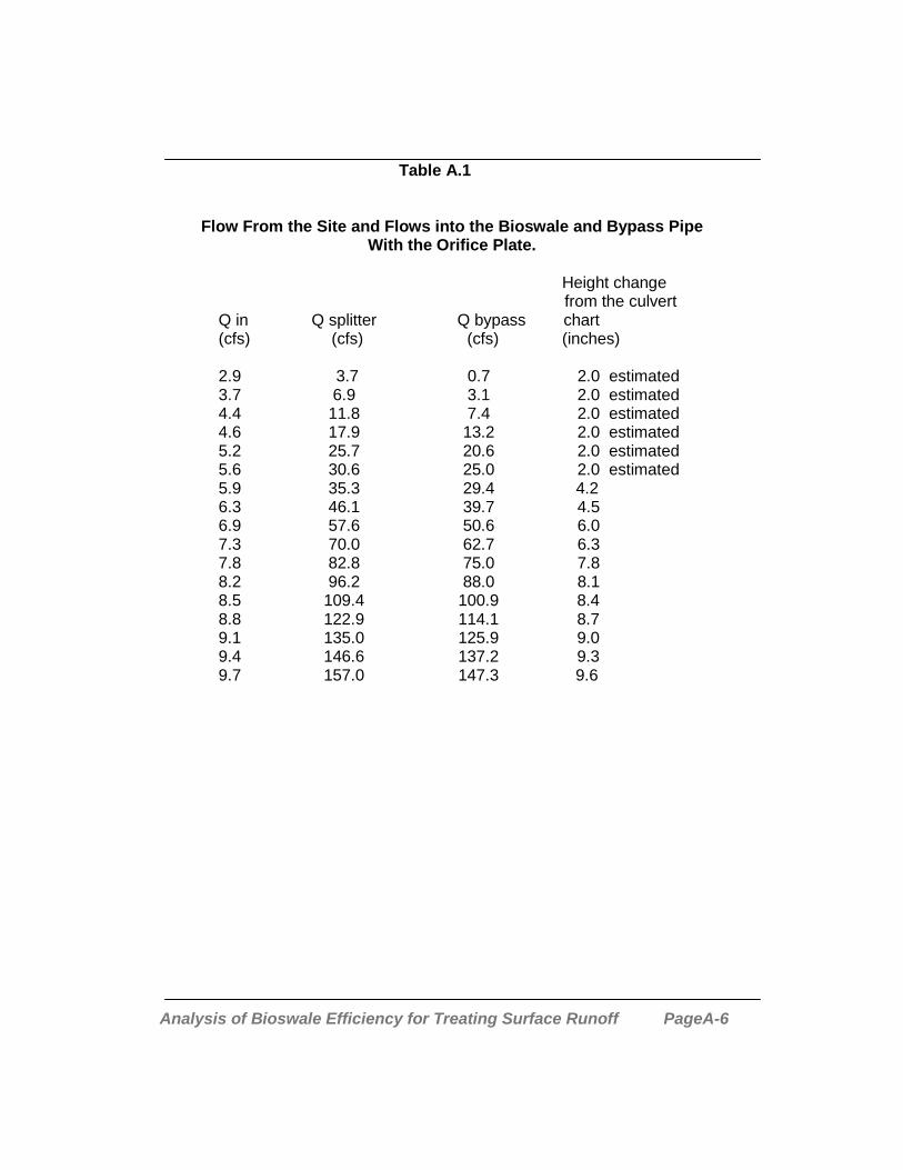
Analysis of Bioswale Efficiency for Treating Surface Runoff PageA-6
Table A.1
Flow From the Site and Flows into the Bioswale and Bypass PipeWith the Orifice Plate.
Height change from the culvert
Q in Q splitter Q bypass chart (cfs) (cfs) (cfs) (inches)
2.9 3.7 0.7 2.0 estimated 3.7 6.9 3.1 2.0 estimated 4.4 11.8 7.4 2.0 estimated 4.6 17.9 13.2 2.0 estimated 5.2 25.7 20.6 2.0 estimated 5.6 30.6 25.0 2.0 estimated 5.9 35.3 29.4 4.2 6.3 46.1 39.7 4.5 6.9 57.6 50.6 6.0 7.3 70.0 62.7 6.3 7.8 82.8 75.0 7.8 8.2 96.2 88.0 8.1 8.5 109.4 100.9 8.4 8.8 122.9 114.1 8.7 9.1 135.0 125.9 9.0 9.4 146.6 137.2 9.3 9.7 157.0 147.3 9.6

Analysis of Bioswale Efficiency for Treating Surface Runoff PageA-7
Table A.2
Flows Exiting the Energy Dissipator
Energy dissipatorObserved Velocity of Flow Field FlowExitingHeight H (ft) approach V (ft/s) Exiting (cfs) H (ft) (cfs) 0.12 2.0 0.3 0.13 (1.5”)* 0.3 0.21 2.6 0.7 0.30 3.1 1.2 0.46 (5.5”) 2.3 0.55 4.2 3.0 0.63 (7.5”) 3.6 0.81 5.1 5.2 1.04 5.8 7.9 1.31 6.5 10.9 1.57 7.1 14.2 1.79 7.6 17.8 1.83 (22”) 18.4 2.04 8.1 21.6 2.0 (24”) 21.0 2.30 8.6 25.7 2.57 9.1 30.1 2.80 9.5 35.0 3.04 9.9 47.1 3.29 10.3 64.0 3.56 10.7 84.3 3.83 11.1 107.3 4.32 11.8 132.8
*Field Measurements were taken in inches and rounded to the nearest ½ inch.

Analysis of Bioswale Efficiency for Treating Surface Runoff PageA-8
Table A.3Storage-Outflow Relationship for the Bioswale
Water Above Storage Above the Rate of Outflow S/∆t (s(t)-o/2) (s(t)+o/2)The exit pipe bottom of the exit pipe (cfs) (cfs) (cfs) (cfs) (ft) (ft3)
0.10 857 0.08 0.95 0.91 0.99 0.20 1291 0.33 1.43 1.27 1.60 0.30 1849 0.78 2.05 1.66 2.44 0.40 2558 1.41 2.84 2.14 3.55 0.50 3419 2.21 3.80 2.69 4.90 0.60 4315 3.12 4.79 3.23 6.35 0.67 5168 3.90 5.74 3.79 7.69 0.72 5790 4.50 6.43 4.18 8.68 0.77 6434 5.00 7.15 4.65 9.65 0.81 6964 5.50 7.74 4.99 10.49 0.88 7974 5.90 8.86 5.91 11.81 1.42 16784 10.9 18.65 13.20 24.10 2.00 26291 14.9 29.21 21.76 36.66
Table A.4 Hydrograph Routing Through the Bioswale
Time Inflow Average Inflow (S1/∆t –O1/2) (S2/∆t –O2/2) Outflow(minutes) (cfs) (cfs) At beginning of At end of time (cfs) time interval (cfs) interval (cfs)0 0 - - - 0.015 1.0 0.5 0.5 0.030 1.5 1.3 0.0 1.3 0.245 4.5 3.0 1.1 4.1 1.760 6.0 5.3 2.0 7.3 3.475 7.0 6.5 3.5 10.0 5.290 8.5 7.8 4.8 12.6 6.2105 9.0 8.8 6.3 15.1 7.2120 9.0 9.0 7.8 16.8 7.9135 7.5 8.3 8.8 17.1 8.1150 4.0 5.8 9.1 14.9 7.2165 2.2 3.1 7.8 10.9 5.7180 1.4 1.8 5.4 7.2 3.6195 1.0 1.2 3.6 4.8 2.1210 0.7 0.9 2.7 3.6 1.5

Analysis of Bioswale Efficiency for Treating Surface Runoff PageA-9
Table A.5
Flow From the Site into Bioswale and Bypass Pipe Without the Orifice Plate
Q in Q bypass Q splitter(cfs) (cfs) (cfs)
2.3 0.0 2.3 5.5 0.0 5.5
5.9 0.7 6.6 10.9 3.1 14.0 14.9 7.4 22.3 18.4 13.2 31.6 21.4 20.5 41.9 24.1 25.0 49.1 25.8 29.4 55.2 28.2 39.7 67.9 31.1 50.6 81.7 33.2 62.7 95.9 35.7 75.0 110.7 36.4 88.0 124.4 37.1 100.9 138.0 37.9 114.1 152.0 38.7 125.9 164.6 39.5 137.2 176.7 40.3 147.3 187.6

Analysis of Bioswale Efficiency for Treating Surface Runoff PageA-10
Table A.6Depth-Volume-Outflow Relationships for Bioswale Forebay, Bioswale Backbay and
Natural AreaUnit Depth (ft.) Surf. Area
(sq. ft.)Volume(cu. ft.)
Treated Outflow (cfs)
0.00 0.00 0.00 0.00
0.50 2860 1430 0.11
1.00 2860 2860 0.47
1.50 2860 4290 0.71
2.15 2860 6149 1.51
2.20 2860 6292 2.47
2.22 2860 6349 2.92
2.25 2860 6435 3.69
2.27 2860 6492 4.25
2.30 2860 6578 5.14
2.35 2860 6721 6.79
2.40 2860 6864 8.61
2.45 2860 7007 10.59
2.50 2860 7150 12.72
2.60 2860 7436 17.38
Bioswale Forebay
2.70 2860 7722 22.53
0.00 0.00 0.00 0.00
0.25 2851 537 0.00
0.75 9280 3419 2.21
1.00 12865 6155 4.70
Bioswale Backbay
1.05 15639 6820 5.40
0.00 11484 0.00 0.0
1.00 29387 19747 12.4
2.00 41831 55174 32.3
3.00 50439 107140 43.3
4.00 60191 176897 52.1
6.00 86480 362639 98.5
7.00 163954 510937 137.3
Natural Area
8.00 230492 735449 186.4

Analysis of Bioswale Efficiency for Treating Surface Runoff Page B-1
Appendix B
Table B.1Bioswale Plant List
Planting Area Scientific name Common Name
Forebay Eleocharis palustris Spike RushAnemopsis californica Yerba ManzaLilium pardolinum Water Lilly
Backbay Scirpus maritimus Bull RushScirpus californica Bull Rush
Distichlis spicata Salt GrassJuncus patens Common Rush
Cyperus eragrostis Common CyprusJuncus phaeocephalus Brown Headed Creeping Rush
Dam Artemesia californica California SagebrushBaccaris pilularisDiplacus duranliucus MonkeyflowerElymus condensatus Giant Ryegrass
Bank Plantanus racemosa Western SycamorePopulus fremonti Fremont CottonwoodAcer negundo BoxelderQuercus agrifolia Live OakPrunus lyonii Catalina CherryGeteromeles arbutifoliaRhus integrifolia Lemonade BerryNassella pulchra Purple NeedlegrassBerberis nevinii BarkberryRubus ursinus California BlackberryArtemesia douglasii MugwortRosa californica California Wild Rose

Analysis of Bioswale Efficiency for Treating Surface Runoff Page B-2
This page intentionally left blank

Analysis of Bioswale Efficiency for Treating Surface Runoff Page D-1
Appendix DChemical Sampling DataTable D.1. Water Sampling Data from 11/7/98 Sampling Event at K-Mart.
Date 11/7/98Sample I.D. K-Mart 1 K-Mart 2 K-Mart 3 K-Mart 4Time 4:20 p.m. 5:24 p.m. 5:40 p.m. 6:00 p.m.Avg. Flow (cfs) 0.005 0.029 0.058 0.032
K-MartConstituent Test Method Detection Limit EMCTPH (mg/L) EPA 418.1 10 3 7.6 7.1 2.1 6Lead (mg/L) EPA 200.8 0.005 0.01 0.013 0.014 0.008 0Total P as Phosphorous (mg/L) SM 4500-P 0.2 4 5.7 14 8 10Total P as Phosphate (mg/L) SM 4500-P 0.6 12 17 42 24 30Total Alkalinity (mg/L) CaCO3 EPA 310.1 5.0 66 110 74 82 84Calcium (mg/L) EPA 200.8 0.5 86 51 50 35 48Chloride (mg/L) EPA 300.0 0.5 320 740 260 84 329Hardness (mg/L) CaCO3 Calculation 5.0 320 220 190 130 187Magnesium (mg/L) EPA 200.8 0.1 26 25 16 8.8 17Nitrate (NO3-N) (mg/L) EPA 300.0 0.5 6.2 2.4 2.4 2 2Nitrite (NO2-N) (mg/L) EPA 300.0 0.5 0 0 1.1 0.5 1pH EPA 9040 - 7.1 7.3 7.2 7.2 7Potassium (mg/L) EPA 200.8 0.5 27 26 43 27 34Sodium (mg/L) EPA 200.8 0.5 220 180 110 46 114Conductance (umhos/cm) EPA 120.1 1.0 1500 2800 1200 620 1437Sulfate (mg/L) EPA 300.0 0.5 130 140 99 49 97Total Dissolved Solids (mg/L) EPA 160.1 5.0 1400 1900 1200 570 1209Total Suspended Solids (mg/L) EPA 160.2 5.0 20 18 18 41 24

Analysis of Bioswale Efficiency for Treating Surface Runoff Page D-2
Table D.2. Soil Sampling Results for Composite Forebay Soil Collected on 1/19/99.
O nta rio M in is try o f E nvironm en t and F orebay W iscons in D ep t. o f N a tura l R esou rces C om pos ite R esu lts
S ed im en t Q ua lity C rite ra C onstituen t m g /kg (ppm ) m g /kg (ppm )T P H 100 230T o ta l P as P hosphorous 600 700T o ta l P as P hosphate 2100A ntim ony ndA rsen ic 10 ndB arium 61B ery llium ndC adm ium 1 ndC hrom ium 100 16C oba lt 25 6 .9C opper 100 7 .8Lead 50 5 .7M ercu ry 0 .1 ndM o lybdenum 4 ndN icke l 100 95S e len ium 2 ndS ilver 0 .5 ndT ha llium ndV anad ium 16Z inc 100 44nd = no t de tec tedS ource : B audo, e t a l., 1990
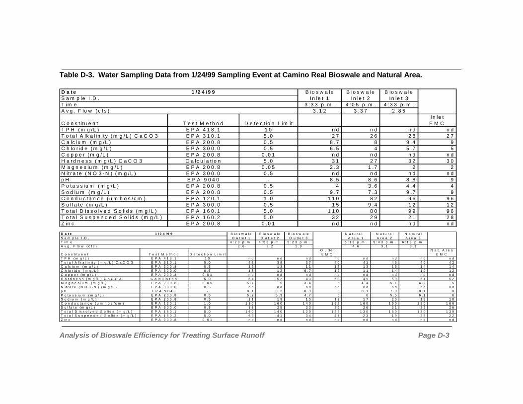
Analysis of Bioswale Efficiency for Treating Surface Runoff Page D-3
Table D-3. Water Sampling Data from 1/24/99 Sampling Event at Camino Real Bioswale and Natural Area.
D a t e 1 /2 4 /9 9 B io s w a le B io s w a le B io s w a leS a m p le I .D . In le t 1 In le t 2 In le t 3T im e 3 :3 3 p .m . 4 :0 5 p .m . 4 :3 3 p .m .A v g . F lo w ( c f s ) 3 .1 2 3 .3 7 2 .8 5
In le tC o n s t i tu e n t T e s t M e th o d D e te c t io n L im it E M CT P H ( m g /L ) E P A 4 1 8 .1 1 0 n d n d n d n dT o ta l A lk a l in i t y ( m g /L ) C a C O 3 E P A 3 1 0 .1 5 .0 2 7 2 6 2 8 2 7C a lc iu m ( m g /L ) E P A 2 0 0 .8 0 .5 8 .7 8 9 .4 9C h lo r id e ( m g /L ) E P A 3 0 0 .0 0 .5 6 .5 4 5 .7 5C o p p e r ( m g /L ) E P A 2 0 0 .8 0 .0 1 n d n d n d n dH a r d n e s s ( m g /L ) C a C O 3 C a lc u la t io n 5 .0 3 1 2 7 3 2 3 0M a g n e s iu m ( m g /L ) E P A 2 0 0 .8 0 .0 5 2 .3 1 .7 2 2N it r a te ( N O 3 - N ) ( m g /L ) E P A 3 0 0 .0 0 .5 n d n d n d n dp H E P A 9 0 4 0 - 8 .5 8 .6 8 .8 9P o ta s s iu m ( m g /L ) E P A 2 0 0 .8 0 .5 4 3 .6 4 .4 4S o d iu m ( m g /L ) E P A 2 0 0 .8 0 .5 9 .7 7 .3 9 .7 9C o n d u c ta n c e ( u m h o s /c m ) E P A 1 2 0 .1 1 .0 1 1 0 8 2 9 6 9 6S u lf a te ( m g /L ) E P A 3 0 0 .0 0 .5 1 5 9 .4 1 2 1 2T o ta l D is s o lv e d S o l id s ( m g /L ) E P A 1 6 0 .1 5 .0 1 1 0 8 0 9 9 9 6T o ta l S u s p e n d e d S o l id s ( m g /L ) E P A 1 6 0 .2 5 .0 3 2 2 9 2 1 2 8Z in c E P A 2 0 0 .8 0 .0 1 n d n d n d n d
D a t e 1 / 2 4 / 9 9 B i o s w a l e B i o s w a l e B i o s w a l e N a t u r a l N a t u r a l N a t u r a lS a m p l e I . D . O u t l e t 1 O u t l e t 2 O u t l e t 3 A r e a 1 A r e a 2 A r e a 3T i m e 4 : 2 3 p . m . 4 : 5 3 p . m . 5 : 2 3 p . m . 5 : 1 3 p . m . 5 : 4 3 p . m . 6 : 1 3 p . m .A v g . F l o w ( c f s ) 2 . 6 2 . 2 1 . 9 4 . 6 3 . 1 3 . 1
O u t l e t N a t . A r e aC o n s t i t u e n t T e s t M e t h o d D e t e c t i o n L i m i t E M C E M CT P H ( m g / L ) E P A 4 1 8 . 1 1 0 n d n d n d n d n d n d n d n dT o t a l A l k a l i n i t y ( m g / L ) C a C O 3 E P A 3 1 0 . 1 5 . 0 4 2 3 9 3 7 4 0 4 1 4 6 4 0 4 2C a l c i u m ( m g / L ) E P A 2 0 0 . 8 0 . 5 1 2 1 3 1 1 1 2 1 3 1 5 1 4 1 4C h l o r i d e ( m g / L ) E P A 3 0 0 . 0 0 . 5 1 3 1 2 9 . 7 1 2 1 1 1 4 1 0 1 2C o p p e r ( m g / L ) E P A 2 0 0 . 8 0 . 0 1 n d n d n d n d n d n d n d n dH a r d n e s s ( m g / L ) C a C O 3 C a l c u l a t i o n 5 . 0 5 4 5 2 4 3 5 0 4 9 5 9 5 1 5 2M a g n e s i u m ( m g / L ) E P A 2 0 0 . 8 0 . 0 5 5 . 7 5 3 . 4 5 4 . 4 5 . 1 4 . 2 5N i t r a t e ( N O 3 - N ) ( m g / L ) E P A 3 0 0 . 0 0 . 5 n d n d n d n d n d n d n d n dp H E P A 9 0 4 0 - 8 . 1 8 . 2 8 . 3 8 8 . 1 7 . 8 8 . 1 8P o t a s s i u m ( m g / L ) E P A 2 0 0 . 8 0 . 5 5 . 2 5 . 3 4 . 7 5 6 5 . 5 6 . 1 6S o d i u m ( m g / L ) E P A 2 0 0 . 8 0 . 5 2 1 1 9 1 5 1 9 1 7 2 0 1 8 1 8C o n d u c t a n c e ( u m h o s / c m ) E P A 1 2 0 . 1 1 . 0 1 8 0 1 6 0 1 4 0 1 6 2 1 6 0 1 9 0 1 5 0 1 6 6S u l f a t e ( m g / L ) E P A 3 0 0 . 0 0 . 5 3 3 2 9 2 3 2 9 2 6 3 1 2 2 2 6T o t a l D i s s o l v e d S o l i d s ( m g / L ) E P A 1 6 0 . 1 5 . 0 1 6 0 1 4 0 1 2 0 1 4 2 1 3 0 1 6 0 1 3 0 1 3 9T o t a l S u s p e n d e d S o l i d s ( m g / L ) E P A 1 6 0 . 2 5 . 0 6 2 4 1 3 4 4 7 2 3 1 9 2 3 2 2Z i n c E P A 2 0 0 . 8 0 . 0 1 n d n d n d n d n d n d n d n d

Analysis of Bioswale Efficiency for Treating Surface Runoff Page D-4
Table D.4. Water Sampling Data from 1/31/99 Sampling Event at Camino Real Bioswale.
Date 1/31/99 Bioswale Bioswale Bioswale Bioswale Bioswale BioswaleSample I.D. Inlet 1 Inlet 2 Inlet 3 Inlet 4 Inlet 5 Inlet 6Time 12:31 a.m. 12:46 a.m. 1:01 a.m. 1:16 a.m. 1:31 a.m. 1:45 a.m.Avg. Flow (cfs) 1.66 1.15 1.15 0.87 0.61 0.33
Constituent Test Method Detection LimitTotal P as Phosphate (mg/L) Flow Inj. Analysis 0.1 uM 19.6 9.7 8.3 9.3 8.2 10.2Nitrate (NO3-N) (mg/L) Flow Inj. Analysis 0.5 uM 69.3 66.9 47.7 74.5 50.5 76.7Nitrite (NO2-N) (mg/L) Flow Inj. Analysis 0.1 uM 7.7 6.2 4.6 7.4 5.4 7.7Ammonia (NH3-N) (mg/L) Flow Inj. Analysis 0.1 uM 194 137 152 167 107 123Copper (mg/L) flame AAS 0.01 mg/L 0.02 0.01 0.01 0.01 0.01 0.01Lead (mg/L) flame AAS 0.03 mg/L 0.16 0.15 0.06 0.06 0.04 0.04Zinc (mg/L) flame AAS 0.005 mg/L 0.018 0.037 0.042 0.071 0.058 0.081Total Suspended Solids (mg/L) EPA 160.2 5.0 641 290 187 250 154 213
Date 1/31/99 Bioswale Bioswale Bioswale BioswaleSample I.D. Outlet 1 Outlet 2 Outlet 3 Outlet 4Time 1:07 a.m. 1:28 a.m. 1:43 a.m. 1:58 a.m.Avg. Flow (cfs) 0.14 0.25 0.25 0.36
Inlet OutletConstituent Test Method Detection Limit EMC EMCTotal P as Phosphate (mg/L) Flow Inj. Analysis 0.1 uM 12 5.7 6.8 6.4 7.3 7Nitrate (NO3-N) (mg/L) Flow Inj. Analysis 0.5 uM 64 42.9 39 45 51.8 46Nitrite (NO2-N) (mg/L) Flow Inj. Analysis 0.1 uM 6 4.2 3.9 5 5.5 5Ammonia (NH3-N) (mg/L) Flow Inj. Analysis 0.1 uM 157 157 146 129 116 132Copper (mg/L) flame AAS 0.01 mg/L 0.01 0.01 0.01 0.01 0.01 0.01Lead (mg/L) flame AAS 0.03 mg/L 0.10 0.06 0.04 0.03 0.01 0.03Zinc (mg/L) flame AAS 0.005 mg/L 0.04 0.037 0.03 0.028 0.032 0.03Total Suspended Solids (mg/L) EPA 160.2 5.0 346 347 411 252 781 495

Analysis of Bioswale Efficiency for Treating Surface Runoff Page D-5
Table D.5. Water Sampling Data from 2/9/99 Sampling Event at Camino Real Bioswale and Natural Area.
Date 2/9/99 Bioswale Bioswale Bioswale Bioswale BioswaleSample I.D. Inlet 1 Inlet 2 Inlet 3 Outlet 1 Outlet 2Time 6:08 a.m. 6:38 a.m. 7:08 a.m. 7:05 a.m. 7:38 a.m.Avg. Flow (cfs) 3.5 3.3 3 2.6 1.9
InletConstituent Test Method Detection Limit EMCTPH (mg/L) EPA 418.1 10 nd nd nd nd nd ndTotal P as Phosphate (mg/L) Flow Inj. Analysis 0.1 uM 4.9 4.3 4.9 5 6 5.6Nitrate (NO3-N) (mg/L) Flow Inj. Analysis 0.5 uM 17.9 12.9 15.8 16 20.8 24.7Nitrite (NO2-N) (mg/L) Flow Inj. Analysis 0.1 uM 1.7 1.4 1.6 2 2 2.4Ammonia (NH3-N) (mg/L) Flow Inj. Analysis 0.1 uM 149 89 152 130 162 92Copper (mg/L) flame AAS 0.01 mg/L 0.04 0.01 0 0.02 0.01 0Lead (mg/L) flame AAS 0.03 mg/L 0.01 0 0 0.00 0 0Zinc (mg/L) flame AAS 0.005 mg/L 0.028 0.018 0.01 0.02 0.028 0.018Total Suspended Solids (mg/L) EPA 160.2 5.0 289 245 271 269 243 235
Date 2/9/99 Bioswale Natural Natural NaturalSample I.D. Outlet 3 Area 1 Area 2 Area 3Time 8:16 a.m. 8:05 a.m. 8:38 a.m. 9:24 a.m.Avg. Flow (cfs) 1 5.2 4.6 5.2
Outlet Nat. AreaConstituent Test Method Detection Limit EMC EMCTPH (mg/L) EPA 418.1 10 nd nd nd nd nd ndTotal P as Phosphate (mg/L) Flow Inj. Analysis 0.1 uM 5.6 6 5.7 4.8 5.3 5Nitrate (NO3-N) (mg/L) Flow Inj. Analysis 0.5 uM 20.9 22 16.7 12.1 19.9 16Nitrite (NO2-N) (mg/L) Flow Inj. Analysis 0.1 uM 2.1 2 1.7 1.3 2 2Ammonia (NH3-N) (mg/L) Flow Inj. Analysis 0.1 uM 88 124 165 97 129 132Copper (mg/L) flame AAS 0.01 mg/L 0 0.01 0 0 0 0.00Lead (mg/L) flame AAS 0.03 mg/L 0 0.00 0.01 0 0 0.00Zinc (mg/L) flame AAS 0.005 mg/L 0.018 0.02 0.013 0.008 0.01 0.01Total Suspended Solids (mg/L) EPA 160.2 5.0 201 233 218 225 215 219

Analysis of Bioswale Efficiency for Treating Surface Runoff Page D-6
This page intentionally left blank
Top Related