


Languages
Pages
Legal

An integrated computer system for engineering problem solving
DANIEL ROOS
Department of Civil Engineering, Massachusetts Institute of Technology Cambridge, Massachusetts
SYSTEM OBJECTIVES
Computers should provide. the mechanism that enables engineers to do better engineeri~g. By permitting faster, more accurate and complete problem analysis to be performed, computers assist the engineer in his computational and decision making roles. The engineer today is faced with problems of increasing magnitude and complexity where the effects and interrelationships of all relevant information must be considered. The computer can provide the coordinating and integrating mechanism for this problem information.
This role of the computer in engineering is only achieved when the computer is adequately integrated in the problem-solving environment. The computer must be properly integrated with both the programmer developing it and the engineer using it.
How is this integration of engineer and computer accomplished? The engineer must do more than use the computer. He must actively participate in the computer solution. To do this he needs a language to communicate with the computer, physical accessibility to the computer, and the ability to obtain engineering oriented results from the computer. The communication language must be oriented to the problem rather than the machine and must allow the engineer to easily specify his problem solving requirements. Accessibility, provided through some type of remote console, permits the engineer to interact with the computer during the problem solution. Meaningful engineeringoriented results are obtained using scopes, plotters and other output devices.
Integration of the programmer and the computer is provided through a powerful programming language
lSl
and the necessary system programs to support the language. The programming language should be dynamic with respect to both problem solution and computer memory requirements. It should allow complete problem solutions where the type and the amount of data can vary. To satisfy these requirements, the system should include dynamic memory allocation, alternate forms of data structure, and a data management and transfer mechanism so that the same data can be used in all aspects of the problem solution.
The Civil Engineering Systems Laboratory at M.I.T. is currently developing a computer system, ICES (Integrated Civil Engineering System) based on the above requirements. It includes a computer programming language, ICETRAN (ICES FORTRAN), oriented toward engineering problem solving, and an engineerfugoriented operating monitor system. These programming aids enable programmers to easily create and modify ICES, which can then be used by the engineer in the solution of engineering problems.
ENGINEERING PROBLEM CHARACTERISTICS
What are the characteristics of engineering problems and how do they affect the design of ICES? The solution of civil engineering problems generally involves the consideration of many disciplines. For example, even in a relatively small problem such as the design of a highway interchange, engineers must consider the highway location and design (highway engineering), settlement, stability, and foundation conditions (soil engineering), highway bridges, (structural engineering), drainage (hydraulic engineering), and traffic flow (transportation engineering). Engineers recognize each of these
From the collection of the Computer History Museum (www.computerhistory.org)
152 An integrated computer system
separate disciplines and the necessary interactions that must exist for effective problem solving. In the past, the complexity of engineering problems and the large amount of data often forced an engineer to unnaturally decompose a problem into noninteractive tasks. Many of the feedback aspects of the problem had to be overlooked.
A computer system such as ICES offers the mechanism to permit complete problem solutions where all factors and interactions are included. In ICES each of the civil engineering disciplines is included as one or more subsystems which may interact with one another. An engineer proceeds in his problem solution by using the necessary subsystems at the proper time. At any point in his problem solution he can leave one subsystem, enter another to perform calculations and then reenter the original subsystem using the results just obtained.
Two engineers given the same problem will quite often arrive at correct yet totally different solutions. Engineering is a creative process, so it is natural to expect a problem solution to reflect an engineer's own experience. The ICES subsystems allow a civil engineer to solve the many different problems that arise, while not constraining his role as a decision maker.
The subsystem design reflects the wayan engineer does engineering. He performs a series of fundamental engineering and mathematical operations to obtain a problem solution. These fundamental operations can be considered basic computational building blocks. Each subsystem of ICES contains a set of building block subroutines. These subroutines, developed by ICES subsystem programmers, are written in ICETRAN, a compiler language somewhat similar to FORTRAN.
The set of basic building blocks alone, however, is not sufficient. The engineer must decide what operations (building blocks) are to be performed (used), the sequence of these operations and the data associated with each operation. It is impractical and undesirable to try to include all these decision making functions in the subsystem computer programs. Instead, they must be specified by the engineer at execution time.
PROBLEM-ORIENTED LANGUAGES
A language is therefore needed to allow the engineer to easily communicate this information to the computer. This language must not be oriented to the programmer as is ICETRAN but instead oriented toward the engineer and the problem he is solving. An engineer should be able to communicate with the computer in much the same way he communicates with another
engineer. He must instruct the machine rather than follow instructions that have been imposed by machine.
The engineering communication language should be command structured where each command represents an operation or group of operations the computer is to. perform. The commands are technical terms which have meaning to the engineer. Each command may also contain data relevant to the requested operations. An engineer must choose which commands to use, the order of their use, and the associated data. Two engineers might solve the same problem using totally different commands. With a command structured language, the quality and efficiency of the computer solution is dependent on the engineering ability of the user.
A command structured language enables the engineer to program a computer without being concerned with programming details. Although the commands result in a program to the computer in that the engineer is "instructing" the computer, they appear to the engineer as a logical problem statement in engineering terminology. Such languages may therefore be referred to as problem-oriented languages.
Two different types of programming languages, each used by a different type of person, are therefore involved in ICES. The ICETRAN language is used by programmers to write ICES subsystem subroutines. Problem-oriented languages are used by engineers at execution time to specify the characteristics of the particular problem being solved.
FORTRAN and other similar languages (lCETRAN) have sometimes been referred to as problemoriented languages. It appears more realistic to refer to these languages as procedure-oriented, and reserve the term problem oriented for a language that satisfies the following requirements:
1. It is oriented to the user rather than the programmer. No computer programming knowledge is required to effectively use the language.
2. The language is command structured where the commands are composed of technical terms.
To avoid further confusion in this paper, it is necessary for the reader to distinguish between a problemoriented language used by an engineer and a procedureoriented language used by a programmer.
The benefits of the problem-oriented language approach have already been demonstrated. CO GO (COordinate GeOmetry) is a problem oriented language used for the solution of geometric problems developed by Professor C. L. Miller of the Department of Civil Engineering at M.I.T. It is interesting to note the impact of COGO on the civil engineering profession since its introduction in 1960. It is used by many state highway
From the collection of the Computer History Museum (www.computerhistory.org)

departments and private consulting firms. One state highway department uses COGO for over 50% of its computer runs. COGO supersedes several hundred special-purpose geometric programs. The use of CO GO has also resulted in increased engineerng productivity and improved engineering design. It has introduced many somewhat reluctant engineers to the computer, and it has produced considerable self-satisfaction among the engineers who have used it. Many engineers have become very frustrated as a result of computer use where they were relegated to filling out cumbersome input forms for use with library programs. COGO allows these engineers to perform engineering while using the computer rather than simply filling out forms. Similar favorable reactions from the profession have also been observed with regard to another problem oriented language STRESS (STRuctural Engineering System Solver), also developed by the Department of Civil Engineering at M.I.T. Past COGO and STRESS work serves as the basis for two subsystems of ICES.
In ICES the engineer formulates his problem solution using the appropriate subsystem commands. The engineer's commands are processed by the ICES executive program which performs the following operations:
Read and encode command. Analyze, convert, and store data. Perform consistency checks. Transfer control to subroutines for command
execution.
The computer solution consists of two phases: the analysis of the command by the ICES executive and the execution of the command using the appropriate computational subroutines. A command is completely processed before the next command is read. The system operates somewhat as an interpreter, where programs that have previously been written in a procedureoriented language and translated to machine language instructions are CALLed.
COMMAND STRUCTURE
With ICES the structure of problem-oriented languages has been generalized so that the same ICES executive program can be used by all ICES subsystems. The command vocubulary of each subsystem differs, but the command structure is identical. A command consists of a command name and data relating to the requested operation~ The following features are included in the command structure:
1. The data are free format, whereby the engineer need not be concerned with cumbersome card column restrictions.
An integrated computer system 153
2. The data associated with a command may be identified by labels and specified in any order. If the engineer prefers, he may omit the labels and enter the data in a standard order. An example of a command with labeled data items to store the X and Y coordinates of point lOis
STORE POINT 10 X 500 Y 750.63
Without labels, the command would be
STORE 10 500 750.63
3. The engineer may omit a command data value and a standard value will automatically be inserted by the executive. This value may be either:
( a) permanently preset by the programmer when the command is initially set up;
(b) temporarily preset by the engineer at the beginning of the problem;
(c) the current value of the data item.
The programmer who initially sets up the command indicates which of these options will be followed. If a standard value is not associated with the data item, the executive will indicate an error condition whenever the data value are omitted by the engineer. The use of standard values reduces the amount of unnecessary data an engineer must include with a command, since input entries are made only when a nonstandard value is encountered.
4. Data values may be alphanumeric as well as numeric. For example, in a geometric problem the quadrant of an angle may be identified as NE, SE, SW, or NW. The executive. will automatically set a switch based on the alphanumeric value given by the user. This switch can then be interrogated by the subsystem command processing routines.
5. Incremental as well as complete processing of the input command is permitted, i.e., if so instructed, the executive will process part of the data, transfer control to execute that portion of the process, and then return to repeat the cycle, continuing until the data are exhausted. Incremental processing minimizes storage requirements when a command contains a variable number of data items.
6. The executive can initialize variables and increment counters that are specified by the programmer at ~ommand definition time. These variables and counters can then be used by the command processing routines.
7. The command data field can contain command name modifiers which permit complicated tree structured commands to be set up by the programmer.
From the collection of the Computer History Museum (www.computerhistory.org)
154 An integrated computer system
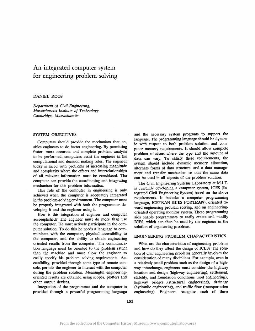
To illustrate command name modifiers, consider the three versions of the INTERSECTION command shown below.
INTERSECTION POINT 5 LINE 10 LINE 20
INTERSECTION POINT 5 LINE 10 ARC 20 NEAR 3
INTERSECTION POINT 5 ARC 10 ARC 20 NEAR 3
The command data consist of the POINT number assigned to the intersection point and the two geometric objects (ARC or LINE) being intersected. In the last two commands, a known point NEAR the desired intersection point must be specified, since a line and an arc can intersect at 2 different points.
The engineer thinks of these as the same command (INTERSECTION); but the programmer must think in terms of three different commands, since each has a different type and amount of data associated with it, and each requires different subroutines for execution. The programmer views the command as the tree structure shown in Fig. 1, where the labels ARC and LINE serve as command name modifiers. These modifiers
Figure 1. The use of command name modifiers.
determine the appropriate branch of the tree and the data and subroutine requirements associated with that branch.
Command name modifiers minimize the number of necessary commands and increase the capabilities of the commands.
COMMAND DEFINITION LANGUAGE
Before an engineer can use a subsystem and its related commands, the subsystem must be added to the ICES system. A set of utility programs are available to perform these modifications. The modifications are performed as normal jobs under ICES, making the system self-modifying. The utility programs include a command definition language which enables a programmer to specify the characteristics of the subsystem commands. This command definition language is a problem-oriented language designed for the program-
mer which automatically generates the command tables used by the ICES executive.
ICES therefore includes a problem-oriented language to generate problem-oriented languages. In addition to generating new problem-oriented languages, the command definition language can be used to easily add, modify, or delete commands from a subsystem that already exists. This ability to easily modify a subsystem is a necessary requirement in engineering organizations where both the problems and the organization itself can change.
The simple example below illustrates some of the features of the ICES executive and the command definition language. The STORE command used to define the X and Y coordinates of a known point will be added to the COGO subsystem of ICES. The STORE command as entered by the engineer could appear as:
STORE POINT 10 X 1000.53 Y 960
The command definition program adds the new command to the COGO vocabulary. The underlined words are the vocabulary of the command definition language and the information in quotes is the input data the programmer supplies.
SYSTEM 'COGO' ADD 'STORE' ID 'P' INTEGER 'NPOINT' REQUIRED ID 'X' REAL 'XCOORD' STANDARD 0 ID 'Y' REAL 'YCOORD' STANDARD 0 EXECUTE'STORE' FILE
SYSTEM specifies the ICES subsystem (COGO) being modified, and ADD specifies the type of modification (addition of a command) and the name of the command (STORE). ID gives the characteristics of the data items associated with the command. One ID entry is required for each of the three data items of the STORE command. The information included as part of the ID entry includes:
1. The identifier for the data item. The identifier defines permissible labels that the engineer can use to label the data items. A permissible label is one that begins with the specified identifier. For example, the identifier of P permits the engineer to use P, PT, POINT, etc., as labels for the point number. The identifiers for the X and Y coordinates given in the second and third ID commands are X and Y.
2. The internal machine representation of the data item (REAL or INTEGER).
3. The symbolic computer location where the data
From the collection of the Computer History Museum (www.computerhistory.org)

item will be stored (NPOINT, XCOORD, YCOORD).
4. The action to be followed if the data item is omitted by the engineer. A REQUIRED data item must be entered by the engineer or an error will be indicated by the executive. The ST ANDARD entry is used to specify a preset data value that will be used by the executive if the data item is omitted by the engineer. Since the coordinates of a point are quite often (0,0) they have been preset to these values in the above example. If the action field of the ID command is left blank (this does not occur in the above example), then the data item will retain its current value if omitted from the command by the engineer.
EXECUTE specifies the subroutine to be entered (STORE) to execute the command, and FILE concludes the command definition. If no errors have been detected, the necessary command tables for the newly defined command will be generated and the command will be added to the CO GO subsystem of ICES. The command definition language enables a programmer to easily incorporate problem-oriented language command input in ICES. These commands can then be used by engineers in the solution of their problems.
ON-LINE OPERATIONS
In certain cases the engineer can use a problemoriented language to write all the commands for a problem solution. It is not always possible or desirable, however, for the engineer to function in this manner. Quite often he will formulate part of the solution and then base the remaining portion on the results of the first part. This mode of operation is incompatible with typical batch processing operations. Instead, the engineer must be able to communicate with the computer in an interactive environment where he can:
Request an operation. Examine his results. Determine the next operation to be performed
based on the previous results. This suggests that a problem oriented language func
tions best in an on-line environment. In this environment the engineer can try many alternate designs and compress into one session the same work that would require many individual sessions in a batch processing mode.
Engineering is typically performed under severe time restraints. The turn-around time problem inherent in batch processing can totally negate the otherwise beneficial results of computers. The engineer needs im-
An integrated computer system 155
mediate access to the computer. He can obtain this accessibility through a remote console. The combination of accessibility of a computer and the communication capability of problem oriented languages provides the engineer with the necessary tools for effectively using the computer in engineering problem solving.
ICES DATA STRUCTURE
An engineer solves a problem by performing operations on data. He collects, reduces, analyzes and evaluates data to arrive at meaningful decisions. The type, amount, and reliability of these data vary considerably from problem to problem. A flexible and efficient computer system such as ICES, therefore, requires a flexible and efficient internal data structure.
It is difficult to classify engineering data since they are of many types and varieties. In some cases only the numeric value of data is important, where, in other cases, hierarchical and structural relationships between the data are also important. Data with different external characteristics require different internal computer representation. Some engineering data are best stored as arrays, others as lists, and others as combinations of arrays and lists. In the past, computer systems have generally been limited to one predominant form of storage (either list or array). ICES has alternate forms of data structure, namely, arrays, lists and array-lists. The programmer chooses the appropriate structure for his data based on considerations such as space requirements, access time, information content, manipulation ability, and system overhead. The alternate forms of data structure allow new representations of engineering problems on a computer.
DYNAMIC MEMORY ALLOCATION
Most engineering data are best represented in a computer in array form. To achieve maximum capability and remove the restrictions presently associated with normal FORTRAN DIMENSIONed array storage, arrays can be dynamically allocated. Dynamic allocation of data achieves the following:
1. Arrays are allocated space at execution time rather than at compilation time. They are only allocated the amount of space needed for the problem being solved. The size of the array (i.e., the amount of space used) may be changed at any time during program execution. If an array is not used during the execution of a particular problem, then no space will be allocated.
2. Arrays are shifted between primary and secondary storage to attempt to optimize the use of primary memory. The programmer need not be concerned
From the collection of the Computer History Museum (www.computerhistory.org)

156 An integrated computer system
with this shifting which is performed by ICES system programs.
Dynamic memory allocation is a necessary requirement for an engineering computer system capable of solving different problems with different data size requirements. The result of dynamic memory allocatio~ is that the size of a problem that can be solved is virtually unlimited since secondary storage becomes a logical extension of primary storage. An explanation of the ICES dynamic memory allocation scheme and an example of its use appear later in this paper.
With ICES, dynamic memory allocation is extended to programs as well as data. Programs are brought into primary memory only when they are needed. The allocation of programs and data is properly balanced so that the use of primary memory is optimized.
The memory allocation problem has been considerably simplified as a result of newly announced third generation computer hardware, in particular, new random access storage devices. The new machines are faster, more powerful, larger and cheaper than their second generation counterparts. The large primary and secondary storage available at reduced prices should increase the size of problems that can be solved on the computer and decrease the cost of the problem solution.
DATA MANAGEMENT Secondary storage can contain one or more data
files associated with the complete problem solution. ICES data management system programs control the organization of these data files. They allow the same data file to be used by all subsystems of ICES, and each subsystem to use different names to refer to the same data file. Variable and array names jn one subsystem are mapped into different variable and array names in the other subsystems. Whenever an engineer switches from one subsystem to a different subsystem, data transfer programs use the mapping function to automatically rearrange the data for the new subsystem.
Data management also allows an engineer to easily operate on data files. He can print, modify, or delete any of his files. The data files can serve as permanent documents of completed problems. Space considerations will of course influence how much information an engineer should keep on secondary storage and for how long this information will be retained.
The data management facility also permits public files to be created so that several engineers can have access to the data ~ to work on the same problem. Suitable protection features are provided to ensure that unauthorized users may not examine another person's files.
ICETRAN PROGRAMMING LANGUAGE
If system programming capabilities such as data management, data transfer, dynamic memory allocation, etc., are to be effectively used by programmen, they must be implemented in a suitable programming system. In ICES, these system programming capabilities are included in the ICES operating system and the ICES programming language. The FORTRAN programming language has been extended into a language called ICETRAN (ICES-FORTRAN) which will be used to program the ICES subsystems. ICETRAN contains all of the FORTRAN statements plus additional capabilities to facilitate the problem solving capabilities of ICES. These additional capabilities are imbedded in the normal FORTRAN structure. No new programming restrictions are imposed on the programmer.
To illustrate ICETRAN, an example will be presented showing how dynamic memory allocation is incorporated in the language. To understand the example, however, it is first necessary to briefly summarize the ICES dynamic memory allocation scheme.
Associated with each dynamic array is one COMMON location known as a codeword-pointer. This location contains the following information about the dynamic array:
1. The size of the array. 2. The residence of the array (primary storage,
secondary storage, or array not yet defined). 3. A pointer to the first location of the array in the
data pool. All dynamic arrays are allocated space in a data pool, which consists of the unused primary memory space during program execution time.
4. The status and priority of the array (used during memory reorganization). Dynamic memory allocation. implies that the array space requirements are constantly changing. If the data pool becomes full and more space is needed, then a memory reorganization must be performed. This reorganization is based on the status (active, released, or destroyed) and the assigned priority (high or low) of the array. A sufficient number of arrays are transferred to secondary storage to make room for new active arrays. If an array on secondary storage is later referenced, it will be brought back into primary memory by ICES system programs.
An ICETRAN subroutine illustrating the use of dynamic memory allocation appears below. This sub-
From the collection of the Computer History Museum (www.computerhistory.org)
routine adds two one-dimensional dynamic arrays (A and B) to form a new dynamic array (C).
SUBROUTINE ADD (N) COMMON A, B, C, . . . . . DYNAMIC ARRAYS A, B, C DEFINE C, N, HIGH DO 1 L= 1, N
1 C(L) = A (L) + B (L) DESTROY A RELEASE B RETURN END
The DYNAMIC ARRAYS statement is used to specify all dynamic arrays. The statement does not cause any instructions to be generated by the compiler. The DEFINE statement is used by a programmer to specify information about a dynamic array that will be stored in the codeword-pointer. The DEFINE statement in the above example causes the size (N) and priority (IDGH) of dynamic array C to be inserted in the codeword-pointer of array C. Dynamic arrays A and B have already been DEFINEd in the subprogram that called subroutine ADD.
The DEFINE statement does not cause allocation of space for the· array. The allocation of space is delayed until the first reference to an array element is made (statement 1). The first time statement 1 is referenced "N + 1" contiguous unused locations in the data pool will be obtained. If they are unavailable, a memory reorganization will occur. The pointer of the codeword will then be set to point to the first of the N + 1 locations. The first N locations are used to store the array, and the N + 1 location contains a backpointer to the codeword. If the array is shifted in the data pool during memory reorganization, the pointer of the codeword is appropriately adjusted.
After the DO loop is completed, array A is destroyed (DESTROY A) and array B is temporarily released (RELEASE B). An array should be destroyed if it is no longer needed and released if it is not presently needed. Intelligent use by the programmer of Destroy and Release statements decreases the likelihood of memory reorganization and increases the efficiency of one when it does occur.
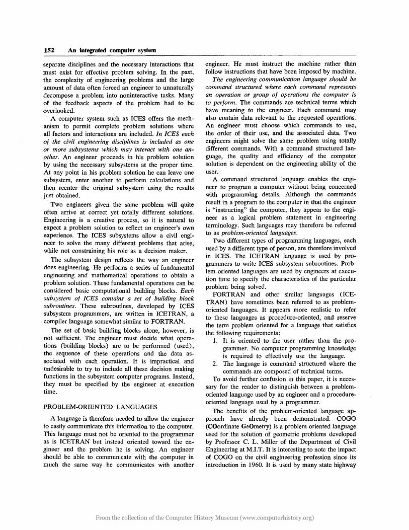
The dynamic memory allocation scheme can handle arrays of any number of dimensions. An n dimensional array is treated internally as a partitioned set of subarrays. This offers extreme flexibility since:
1. Only the sub array an engineer is using need be in core.
2. The size of each subarray can differ. Figure 2
An integrated computer system 157
Figure 2. Array size variation.
shows. a two dimensional array where the size of each sub array (column) varies (2, 4 and 3).
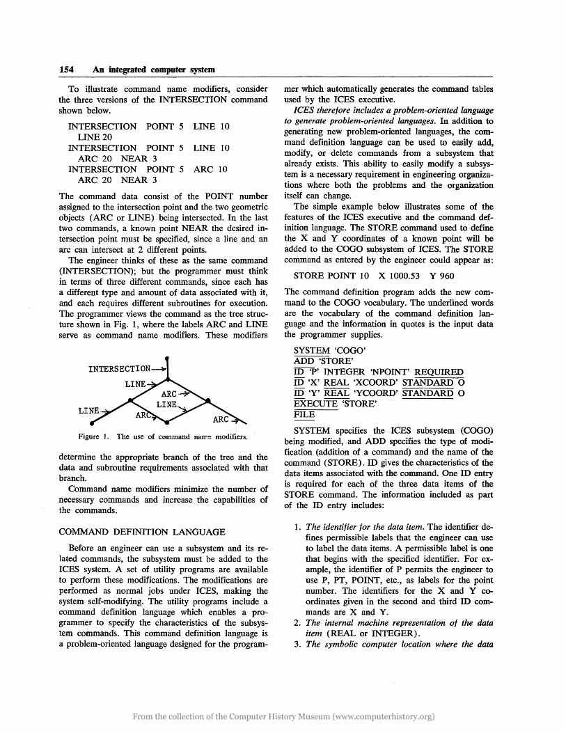
3. The structure of the sub array can vary so that tree structures can be represented using array notation. A tree structure with the associated SUbscript notation is shown in Fig. 3.
The programmer can easily set up a desired struc-
Figure 3. Array structure variations.
ture using the DEFINE command and then operate on the structure using normal FORTRAN array notation.
Dynamic memory allocation capability is merely one of many features available with ICETRAN. Others include list processing, data management, subsystem data transfer, and matrix manipulation.
A completed ICETRAN program must first be processed by the ICES precompiler, which will tt~nslate the ICETRAN statements into legitimate FORTRAN statements. Although the generated FORTRAN statements might appear somewhat confusing to a FORTRAN programmer, they will accomplish the requested operations. The resulting FORTRAN program is then processed by the conventional FORTRAN com .. piler. Use of the precompiler eliminates the necessity of modifying the FORTRAN compiler or developing a totally new programming language.
ICES SYSTEM PROGRAMS
ICETRAN is being developed by people who are experienced in both the information sciences and civil
From the collection of the Computer History Museum (www.computerhistory.org)
158 An integrated computer system
engineering. In the past, a schism has existed between computer language developers and application users. Language developers have not completely appreciated the needs of users, hence their languages were not well suited for the intended users. ICES, however, is developed for civil engineers by civil engineers.
A major difficulty associated with the COGO and STRESS development was the amount of manpower, time, and money that had to be invested to produce the necessary system programs. For example, each language had its own executive routine. There was concern that as more problem-oriented languages developed, the system programming effort would become immense.
One of the goals of ICES was to create the necessary system programs so that programmer-engineers not experienced in system programming could create powerful subsystems. The one set of ICES systems programs are applicable to all the ICES subsystems.
Some people will no doubt express concern about the overhead time of the system programs included in ICES. Quite often, however, an increase in running time is completely justified by the benefits obtained from the operations performed. For example, dynamic memory allocation does involve additional running time, but it also eliminates many bookkeeping requirements and the necessity of packing information. It also increases the problem-solving capabilities.
With ICES, no system programs are forced upon a programmer. He is, for example, given the choice be..,. tween normal dimensioned arrays and dynamic arrays, and between the problem-oriented language input capability and normal FORTRAN READ statements. The programmer must consider the problem being solved and the tradeoffs associated with each of the available alternatives before making his choice.
SUMMARY
Briefly summarizing, ICES contains the following capabilities:
1. Flexible and powerful problem-oriented languages for the engineer to communicate with the computer.
2. On-line capabilities to make the computer accessible to the engineer.
3. An orientation toward complete problem solving, not just computation.
4. An interaction between discipline areas-or subsystems-for solving a problem which encompasses more than one engineering discipline.
5. A data management scheme to organize the data
and a data transfer mechanism to pass the data between subsystems.
6. A modular internal building block structure. 7. An efficient internal data structure where al
ternate forms of data can be represented. 8. Dynamic allocation of data and programs based
on the problem being solved. 9. The ICETRAN programming language to be used
by programmers to develop ICES subsystems.
The first operational version of ICES is currently being implemented on the model 40 IBM System/360 computer in the Civil Engineering Systems Laboratory at M.I.T. The system programs have been written and several subsystems are now being developed. ICES subsystem work should not, however, be restricted to M.I.T. Instead, ICES should be considered as a framework for computer work in civil engineering, where all members of the profession make contributions. It is thus the integrating mechanism for the programs that have been developed in the past and the work that will be performed in the future.
ACKNOWLEDGMENTS
A project such as ICES is the result of careful planning and represents a natural evolution of previous work. For the past 10 years, Professor C. L. Miller, as director of the Civil Engineering Systems Laboratory at M.I.T., has demonstrated how computers can effectively be used in engineering practice and education. This past work serves as the foundation for ICES, which was conceived by Professor Miller and is now being developed by individuals who were trained and inspired by him. These individuals include Robert Logcher, Jay Walton, Alan Hershdorfer, Joe Sussman, Alden Foster, Ron Walter, and Richard Goodman. The work reported in this paper was formulated by these people. The author is also indebted to Miss Betsy Schumacker of IBM and Joel Winett of M.I.T. Lincoln Laboratory for their advice and contributions.
BIBLIOGRAPHY
CHAMPY, J. A., "Man Machine Computer Systems in a Public Works Agency: A Management View," Industrial Management Review, Spring 1965.
FENVES, S. i., et aI, STRESS: A User's Manual, M.I.T. Press, 1964.
FENVES, S. J., R. D. LOGCHER, and S. P. MAUCH, STRESS: A Reference Manual, M.I.T. Press, 1965.
From the collection of the Computer History Museum (www.computerhistory.org)
MILLER, C. L., "Man-Machine Communications in Civil Engineering," M.I. T. Department of Civil Engineering, T63-3 (June 1963).
MILLER, C. L., and R. WALTER, "Communicating with Computers in Civil Engineering Design," M.I.T. Department of Civil Engineering, T65-4. (Mar. 1965).
ROOS, D., and B. SCHUMACKER, "ICES: Integrated Civil Engineering System," M.I.T. Department of Civil Engineering, P65-8 (May 1965).
An integrated computer system 159
ROOS, D., and C. L. MILLER, "COGO-90: Engineering User's Manual," M.I.T. Department of Civil Engineering, R64-12 ( Apr. 1964) .
ROOS, D., and C. L. MILLER, "The Internal Structure of COGO-90," M.I.T. Department of Civil Engineering, LR64-5 (Feb. 1964).
ROOS, D., and C. L. MILLER, "COGO-90 TimeSharing Version, M.I. T. Department of Civil Engineering, LR 64-18 (May 1964).
From the collection of the Computer History Museum (www.computerhistory.org)

From the collection of the Computer History Museum (www.computerhistory.org)
ERRATA
to
Volume 27, Part I
AFIPS Conference Proceedings #(.
1965 Fall Joint Computer Conference
*Published by Spartan Division of Books, Inc., 1250 Connecticut Ave., Washington, D.C.
From the collection of the Computer History Museum (www.computerhistory.org)

From the collection of the Computer History Museum (www.computerhistory.org)

ERRATA to
AFIPS Conference Proceedings
1965 Fall Joint Computer Conference-Part I
(Abbreviations: p. == page; L == left column; R == right column)
w. H.BURKHARDT Universal Programming Languages
p. 2, line 26, L: Change to read in the SEAC machinel) this idea . . .
last line, R: Change to read when relating a machine with 0.5 - microsecond cy -
p. 3, line 1, L: Change to read cle time in 1965 to one with 25 microsecond cycle
p. 4, line 5, R: Change Lanig to Laning line 15, L: Change to read translation of pre
viously ... line 22ff. R: Change to read
3. Time savings in debugging and correcting the programs,
4. Easier modification possibilities for slightly different problems,
5. Higher ... p. 6, line. 22, L: Change to read areas (not vertical
combinations or notations23).
line 33, L: Change to read machines by combination ...
section on "Mathematical Definition and Development" : Replace all subscript numerals 1 by lower case letter tiel."
last line of this section: by an example in reference 28).
second last line, R: Delete 30. p. 7, line 9, R: Change to read IBSYS3l). The ..
line 11, L: Change to read As mentioned in the section on Possible Solutions, there
in section on "Transformation of Programs by Processors": Replace all subscript numerals 1 by lower case letter tiel."
p. 8, line 5 fro below, L: Change to read Language
A into target p. 9, figures: Delete all underlining p. 10, figures: Delete all underlining; change first ar
row to a simple one in each figure in first figure: Change L to ls
p. 11, figures: Delete all underlining; change first arrow to a simple one in each figure
line 14, R: Change (case 1) to (case 31) line 15, L: Change to read -spectively, for
the ... line 15, R: Change (case 2) to (case 32) line 19, R: Change (case 2) to (case 32)
p. 12, Table 1: Move the words Processor in M from TGS row, col. 4, down to Meta A row, col. 4.
p. 13, figures: Change first and third arrow in figure to a simple arrow.
figure on left: Move to end of paragraph p. 14, second row of figures, last figure: Change Ml
to Nt p. 15, figures: Delete all overlines
last figure: Add the angles in the brace p. 16, first figure: Change I N21 to (N2 )
last figure: Change peL) to peL) p. 17, first figure, R: Delete all vertical bars
second figure, R: Change all horizontal arrows to double arrows
last figure, R: Exchange this figure for the first figure on page 18
p. 18, first figure: Exchange this figure with the last figure on p. 17, R
second figure: Insert a simple arrow between M2 and the big X
last figure: Insert a simple arrow between E and the big X
p. 19, line 39ff., L: Change to read the plan is not
From the collection of the Computer History Museum (www.computerhistory.org)

164 Errata
possible and to state the conditions as to which way it would then be possible. But new ideas for solutions and new insights into the problems . . .
lIne 27ff: Insert a big X between the letters:
A ~A D C to give D C B B
TOBEY, BOBROW, and ZILLES Automatic Simplification in FORMAC
p. 38, footnote, R: Change called to call p. 39, line 31, L: Change (1 + Z**N to (1 + Z)**N p. 40, line 38, L: Change to read 30 years
line 30, R: Invert the factor!? to read £ C D
line 31, R: Insert == after cp p. 42, line 22, R: Change A == 0 to A ¥= 0
line 31, R: Second n belongs above l line 33, R: Both j == 1 belong under l line 34, R: j ¥= k belongs under second j == 1 line 36, R: Bj belongs close to first n
p. 43, line 43, L: Change to read unexpanded line 32, R: Change script "e1" to lower-case
italic "el"
p. 44, line 8, L: Place arrow after A j
line 8, R: Change optional to optimal line 36, R: Change to read transformation line 40, R: Insert parenthesis between * and C
p. 45, lines 20 and 21, R: Should begin with the symbol ~
p. 46, last line, L: Change first of to or line 14, R: Change of to or
p. 47, line 7, L: Change K to lower-case k line 10, L: Insert i at end of line line 24, L: Change t to i line 5, R: Insert a dot over the * and delete
the dot over the 5 line 6, R: Insert a dot over the * and delete
the dot over the 5 line 11, R: Insert dots over the *BC line 42, R: Change t to i
p. 48, line 6, L: Change both t to ~; P should point to +
line 7,- L: Change t to i line 13, L: Change both.. t to i line 18, L: Change both t to ~ line 19, L: Change t to i line 37, L: Change t to ~ line 38, L: Insert a dot over the second * and
the W; change t to i p. 48, line 38, L: Delete the dot over the 2
line 12, R: Change t to i p. 50, line 12, L: Change to read identical
line 14, L: Insert right parenthesis after numeric line 15, L: Change to read * ABC K 2] where
Kl and K2 are numbers; line 17, L: Change SI X to read SINX line 23, L: Change both t to t line 24, L: Change both t to i line 27, L: Change t to i line 4, R: Delete left parenthesis before COS(A) line 45, R: Change t to i
p. 51, line 25, L: Change t to i line 31, L: Change t to i line 22, R: Insert i after Kl line 23, R: Change t to i line 36, R: Change UTSIM to AUTSIM
p. 52, line 22, R: Change first and to or line 44, R: Change is to in
B. J. KARAFIN New Block Diagram Compiler
pp. 60-61: Correct entries in Table 1 as follows:
Block Type
ACC
FLT
AMP QNT
LQT
SQT FOP
Function Accumulation
Transversal filter
Amplifier Quantizer
Linear quantizer
Square root Floating point
to integer conversion
Output
Pp -I Xk_1P 1 2
1:=0
Y=PIX PI in the number of representative
levels. The representative levels are P2,P."",P2pl" The decision l~vels are Ps,Ps"",P2pl-l"
Y = ( ~) rounded up. Pl.
y=yx
S. P. FRANKEL mdJ. HERNANDEZ Precession Patterns in Delay Line Memories
p. 99, line 21, L: Change 10 to 106
D. N. SENZIG and R. V. SMITH Computer Organization for Array Processing
p. 117, title, remove asterisk and footnote at bottom left
From the collection of the Computer History Museum (www.computerhistory.org)
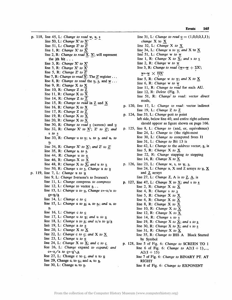
p. 118, line 45, L: Change to read w, u, s line 50, L: Change Xi to Xi - - -line 51, L: Change Zi to Zi line 1, R: Change .Xl to Xi line 2, R: Change to read X. Xlj will represent
the jth bit . . . - -line 3, R: Change Xi to Xi line 3, R: Change Xl to Xi line 5, R: Change Zi to Zi line 7, R: Change to read Xi. The Zl register ... line 8, R: Change to read the !:!' ~, and y!. ••. line 9, R: Change X to X line 10, R: Change Z to Z line 11, R: Change X to X line 14, R: Change Z to Z line 15, R: Change to read in Z and X line 16, R: Change X to X - -line· 17, R: Change Z to Z line 19, R: Change X to X line 20, R: Change X to X line 30, R: Change to read ~ (screen) and !:! line 32, R: Change Xi to Xi; Zi to Zl; and
s to s line 33, R: Change u to ~; Si to ~i and Ui to
~i line 34, R: Change Xi to Xi; and Zi to Zi line 35, R: Change Sl to i -line 44, R: Change u to !:!.. line 46, R: Change. X to X line 48, R: Change X to X; and u to !! line 50, R: Change s to s, Change u to u
p. 119, line 7, L: Change u to ~ -line 9, L: Change Iversons's to Iverson's line 11, L: Change compress to compress line 12, L: Change to vector !! ... line 13, L: Change u to ,!!, Change c~u/a to
£.~y/! line 14, L: Change c to £ line 15, L: Change a to ~ ai to ~l; and u. to
line 16, L: Change c to .£ line 17, L: Change u to y; and u to !!. line 18, L: Change a to .!; and u/a to y/~ line 19, L: Change a to a line 20, L: Change X to X line 22, L: Change c to c; and X to X line 23, L: Change u to ~ -line 24, L: Change X to X; and c to £. line 26, L: Change expand to expand; and c~u/a to £~y~
line 27, L: Changec to £, and u to y line 29, Change Ct to ~; and ai to !i line 30, L: Change Ul to !:!i
Errata, 165
line 31, L: Change to read ~ == (1,0,0,0,1,1); change X to X
line 32, L: Change X to X line 34, L: Change u to u; and X to X line 51, L: Change w to-Y!.. -line 1, R: Change X to X; and s to §.
line 2, R: Change w to Y!.. line 3, R: Change to read (~~~ + IXi;
i
w~w X IIXi
- - 1-
line 5, R: Change w to ~; and X to X line 6, R: Change w to ~ line 11, R: Change to read for each AU. line 12, R: Delete (Fig. 3. line 51, R: Change' to read: vector direct
mode, p. 120, line 17, L: Change to read: vector indirect .
line 19, L: Change Z to ~ p. 124, line 33, L: Change poit to point
left side, below line 40, and entire right column should appear as figure shown on page 166.
p. 125, line 8, L: Change to (and, or, equivalence) line 24, L: Change to (the right-most line 30, L: Change to computed from 11 line 31, L: Change to Bit 13 is line 42, L: Change to the address vector, !, is line 5, R: Change X to X line 22, R: Change stapping to stepping line 14, R: Change X to X
p. 126, line '23, L: Change w, s, to W, .§,
line 24, L: Change u, X and Z arrays to \!, X and Z. arrays
line 27, L: Change Z, A is to '!:., A, is p. 127, line 47, L: Change X to X; and s to !
line 2, R: Change X to X line 4, R: Change s to.! line 5, R: Change X to X line 6, R: Change X to X line 8, R: Change X to X line 10, R: Change X to X line 12, R: Change X to X line 14, R: Change s to ~ line 19, R: Change X to X; and s to].. line 30, R: Change X to X; and s to ~ line 31, R: Change X to X line 35, R: Change to BSS A Block Started
by Symbol p. 128, line 5 of Fig. 6: Change to SCREEN TO 1
line 6 of Fig. 6: Change to A2(1 + 1), ... , A2(1 + 15)
line 7 of Fig. 6: Change to BINARY PT. AT RIGHT
line 8 of Fig. 6: Change to EXPONENT
From the collection of the Computer History Museum (www.computerhistory.org)
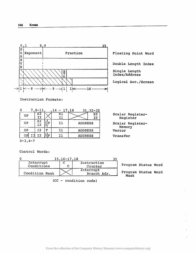
166 Errata
Fraction
--16 >1
Instruction Formats:
o 7,8-11,
'-I -OP X2 12 ,
0-3;4-7
Control Words:
o Interrupt Conditions
Condition Mask
- 17,18 32-35 Xl XO II 10
II ADDRESS
II ADDRESS II ADDRESS
15,16-17,18 C Instruction
C Counter
[X Interrupt Branch Adr.
(CC - condition code)
Floating Point Word
Double Length Index
Single Length Index/Address
Logical Acc./Screen
Scalar Register-Register
Scalar Register-Memory
Vector
Transfer
35
Program Status Word
Program Status Word Mask
From the collection of the Computer History Museum (www.computerhistory.org)
line 10 of Fig. 6: Change to B ( 1) to ELEMENTS
line 11 of Fig. 6: Change to B(A2(1», B(A2 (I + 1»,
line 12 of Fig. 6: Change to A2 + 1,2,,1 ADD A2(1 + 1),A2(I + 2), ... , A2(1 +- 16)
line 13 of Fig. 6: Change to A2-1,2,,1 ADD A2(1- 1),A2(1), ... ,A2(1 + 14)
line 15 of Fig. 6: Change to A2(1 + 1), ... , A2(1 + 15) .
F. J. CORBATO and V. A. VYSSOTSKY Introduction and Overview of Multics System
p. 186, line 6, R: Change Refs. 23 and 24 to Refs. 42 and 24
p. 190, line 45, L: Change more compilations. to more compilation time.
p. 196: Insert at bottom, Ref. 42 as: A. L. Samuel, "Time-Sharing on a Computer," New Scientist 26, 445 (May 27, 1965) 583-87.
E. A. BOWLES The Role of the Computer
p. 270, line 51, L, last word: Change oppositions to opposition
line 10, R: Change kowing to knowing line 15, R: Change Blender to Blendor line 20, R: Delete Old
p. 272, lines 38 and 39, L: Reverse their order line 6, R: Insert comma after tables
p. 273, line 18, R: Change separate to different p. 276, line 3, R: Change Pres to Press
line 11, R: Italicize and capitalize Ibid
D. C. CLARKE and R. E. WALL An Economical Program •••
p. 313, footnote to Table 1: Should be associated with Table 4, p. 314.
ZWICKY et al MITRE Syntactic Analysis Procedure
p. 320, lines 43-47,R and p. 321, lines 1-4, L: Correct format to read as follows: Phrase Structure Component:
75 rules
Errata 167
approximately 275 subrules Transformational Component:
13 initial singularies 26 embeddings and related
singularies, including 9 embeddings
15 final singularies 54 rules
p. 321, line 34, L: Change placement of OPEN to read
PRES sa VTR
OpkN p. 322, line 17-19, L:
(A) ADRIS n
B~ lA
Add lines to diagrams to read (1 B C) SUB n
/\1 231
p. 322, line 26, R: Correct "Checking by Synthesis" as secondary heading (as in line 18), italized, flush left, and with following text entered with paragraph indentation.
p. 323, line after line 12, R: Insert "OTHER APPROACHES TO THE ANALYSIS PROBLEM" as major heading (as in line 26, L above-"Areas for Further Investigation") above "Analysis by Synthe-sis"
p. 325, lines 12-29, L: Correct format to read: (Forward) Grammar
Phrase Structure Component: 61 rules
105 subrules Transformational Component:
Surface Grammar
Reversal Rules
R. C. MINNICK Cobweb Cellular Arrays
11 initial singularies 6 embeddings and related
singularies, including 2 embeddings
3 final singularies 20 rules 32 rules
306 subrules 6 final singularies
15 embeddings and related singularies
11 initial singularies 32 rules
p. 328, line 8, L: Change index to Index p. 329, caption for Fig. 2: Change one to One p. 329, caption for Fig. 3: Should read Cutpoint Reali
zation for a Three-Bit Parallel Adder p. 330, caption for Fig. 4: Should read Cutpoint Reali-
From the collection of the Computer History Museum (www.computerhistory.org)

168 Errata
zation for a Five-Bit Shift Register caption for Fig. 5: Should read Cutpoint Reali
zation for Three Functions of Three VariabIes
p. 331, caption for Fig. 6: Should read Structure of the Cobweb Array
p. 332, caption for Fig. 7: Should read Diode-Transistor Realization of Cobweb Cell
line 17, L: Poorly printed word is cutpoint p. 333, Eq. (3): Replace (j with EB
line 1, R: Replace (j with EB p. 334, caption for Fig. 8: Should/read Shannon and
Reed Decompositions Using Cobweb Arrays p. 335, caption for Fig. 9: Should read Cobweb
Realization for a Three-bit Parallel Adder caption for Fig. 10: Should read Cobweb
Realization for a Five-Bit Shift Register p. 336, line 21, R: Change focal to local
caption for Fig. 11 : Should read Cobweb Realization for Three Functions of Three Variables
caption for Fig. 12: Should read Cobweb Supercells
p. 337, caption for Fig. 13: Should read Exhaustive Listing of the Cobweb Array Fault-Avoidance Algorithm
p. 338, caption for Fig. 14: Should Read Block Diagram for a Twelve-Bit ·Serial Multiplier
p. 339, caption for Fig. 15: Should read Reali~ation of the Multiplier in Terms of Five Cutpoint Arrays
p. 340, caption for Fig. 16: Should read Realization of the Multiplier in Terms of One Cobweb Array
R. H. CANADAY Two-Dimensional Iterative Logic
p. 343, line 23, R: Change to AB + Ac + Be p. 344, line 17, R: Change to r(xl, ... ,xn) == f(xl, ... ,Xn) p. 345, line 17, L: Change Xf/ to Yf/ p. 346, line 25, R: Change C to C-
line 26, R: Change C to C and U to U line 27, R: Change U to U line 33, R: Change to fSd == BCDU + ABCnU
+ ABCD + ABCD + ABC line 34, R: Change to + ABeU +ABCU
+ ABCDU + BDU + COU . p. 349, line 11, L: Change {B,B,U,U} to {B,B,U,U}
line 31, L: Change {C,C,O,I} to {C,C,O,I} line 7, R: Change (n-l to (n-l) line 22, R: Change to gt == BCgtoo + BCgtot +
BCgll0 + BCg111
Array 5, R: Change element 1,6 from B to C
p. 350, Array 7, R: Change element 2,6 from gU01 to g1100
line 15, R: Change A + B to A EB B line 16, R: Change + C +D to EB C EB D
p. 351, line 4, L: Change to {xt,x1x2,x2, ... ,x(n-l),U,U) (U,U) being
Array left boundary, L: Change all 'V to U
p. 352, line 17, L: Change UU to UU line 18, L: Change UgOd to UgOd
line 19, L: Change UU to UU line 20, L: Change Ug1d to Ug /
line 5, R: Change UgOd to UgOd
line 6, R: Change Ug / to Ug /
line 10, R: Change UU to UU line- 22, R: Change to go sd == URogoo + USog01
+ URogd 01 + USot 00 + URoSo line 24, R: Change to glsd == URtg10 + UStgll
+ URlglld + USlglOd + URlS1
line 29, R: Add the term VXRoSo line 30, R: Change to + VYS1gU + VYRtS1
+ WXRltll + WXSlGd lO line 31, R: Change gOl to tOl and goo to too line 33, R: Change UU to DU line 35, R: Change UU to Vu; following that
line should be the heading SUMMARY line 41, R: Change AB+AC+BC to AB+
AC+BC
p. 353, line 1: Eliminate SUMMARY
R. A. SHORT Two-Rail Cellular Cascades
p. 360, line 12, R: Change f to r line 15, R: Change f to f
p. 361, lines 4, 5, 6 L, eq. for f (x!)'''' xn): Change all + to EB
line 10, L: Change f2: (Y2, Y2 + XY1) to f2: (Y2, Y2 EB xYt)
line 20, L, eq. for N: Change (+) to e) line 7 from bottom, R: Change + to EB
p. 362, line 3, L: Change + to EB line 5, 6, 7 from bottom, L: Change all + to
EB line 2, R: Change e~3) to ('1)
p. 363, line 2, 3 from bottom, L: Change all + to EB
p. 365, line 5, 6 from bottom, R: Change all + to EB
p. 367, Fig. 11 (f): Change gz to Y2
From the collection of the Computer History Museum (www.computerhistory.org)
G.E.ROUDABUSHd~
Left Hand of Scholarship • • •
p. 399, line 2, title: Change MEDIA to MEDIUM p. 401, line 39, L: Omit the
line 33, R: Space between we and received p. 402, line 2, L: Change PC to PC6 p. 403, line 6, L: Change printd to printed p. 404, line 16, R: Change gold to bold p. 405, line 2, L: Change slit to split p. 406, line 20, L: Change in our office to done
line 11, R: Omit that line 12, R: Change dattum to datum
p. 408, line 13, L: Change see to set
D. ROOS An Integrated Computer System • • •
p. 424, Fig. 1, R: Distance of 500.26 left out in figure p. 426, line 50, L: Change sybsystems to subsystems p. 427, line 38, R: Change DO I L == 1, I to DO 1 L
== 1, I p. 428, line 6, R: Change DOP to DO p. 430, line 38, R: Change 'N POINT' to 'NPOINT' p. 432, line 8, L: Change System 360 to System/360
line 11, L: Change System 360 to System/360 p. 433, line 5, R: Replace line in 4 with name R. D.
Logcher
C. W. ADAMS Responsive Time-Shared Computing • • •
p. 486, line 6, R: Should follow line 8
L. W. COTTEN Circuit Implementation • • •
p. 489, line 19, L: Change 23 to 20 p. 491, line 32, L:
n-k
P12 == l AtBi +k 1=1
p. 492, line 36, L: Change NOR-OA to NOR-OR line 27, R: Change f == AB to f == Ali line 28, R: Change + AB to + AB
p. 494, line 2, L: Change (X) to (X) line 36, L: Change (Xl -) to (Xl -) line 34, R: Change G to G line 35, R: Change to G: == C - .c. + D + A line 41, R: Change to G: == H - H + I + E
p. 495, line 5, L: Change to Q == K - K + M + T line 18, L: Change T to T
Errata 169
line 19, L: Change T to 1: line 23, L: Change to g == 3T - T line 24, L: Should read As T is made to ap-
proach I, G will approach Q, line 25, L: Change G to G line 26, L: Change to G. == 2T line 42, L: Change 4T to 4T line 7, R: Change 4T to 4T line 25, R: Change our to out line 27, R: Change (Xl) to (Xl)
p. 497, line 6, L: Change 4T to 4!; and where T to where I
line 12, L: Should read alter T and T line 10, R: In two places change 4T to fi line 12, R: Should read 3T - I line 18, R: In both places change to 3T - T line 22, R: Should be 3T - I
Change 4T to 4I line 23, R: Change TIT to TIT line 24, R: Change T to T line 27, R: Change 4T to 4T line 28, R: Change T to T line 30, R: Change T to I; and TIT to TIT line 32, R: Change T == to T ==; and 3T to 3T line 33, R: Change TIT to TIT line 39, R: Change T to T line 43, R: Change T to I. line 45, R: Change T to I
p. 498,. line 42, L: Should read clock system of w.. == line 4, R: Change to (Tl + T2 + Ta + T.) line 7, R: Change (4T) to (4I) line 11, R: Should read .I. == 2.0 line 17, R: Change to (T1 + T2 + Ta) - I line 23, R: Should read has negligible T - T line 26, R: Should be (T2 + Ta) line 27, R: Should read with negligible T - I
p. 499, line 4, L: Should read W2 == 4I. - W1 == 41 - We - Se
line 9, L: Should read of 4 I. + Z; and delay is Sc + 4T + Z .
line 10, L: Should be Wa == (Sc + 4T + Z) - (4I.+ Z)
line 11, L: Should be == 4(T - I) + Sc line 13, L: Change W4 to WI line 15, L: Should be
1
- (We +2Sc)+ (4!-Wc- Sc) +4(T-I) line 18, L: Should read When 41 line 22, L: Change to f == II (Sc + 41') line 23, L; Should read When 4I line 25, L: Change term (T - T) to (T - I) line 27, L: Change If 4T to If 41
From the collection of the Computer History Museum (www.computerhistory.org)
170 Errata
Change then T == to then I == line 28, L: Should read If this I. is line 30, L: Change both 4T terms to 4T line 31, L: Should be It is seen that I line 33, L: Should be When 4I line 36, L: Change 4T to 4:[ line 2, R: Change both 4T terms to 4I line 4, R: Change 4T term to 4T; Should read
speed T might line 6, R: Should read If T == 4.5, I. == 2.5, line 10, R: Change term 4T to 4T line 11, R: Change term in parens to (T - I) line 15, R: Should read such that the r.
p. 503, line 26, R: Change Relay to Delay line 29, R: Change T to T line 31, R: Change T to T line 35, R: Should read X: Logic sense line 38, R: Should read X: Minimum value
G. H. BALL Data Analysis in the Social Sciences • • •
p. 533: Delete entire left column, replacing the two existing paragraphs with the three following paragraphs:
The advent of the relatively inexpensive digital computer makes iterative cluster-seeking methods of analyzing complex multivariate data practical when they could not be seriously considered before. These "cluster-seeking" techniques provide a way of viewing multivariate data that differ from factor analysis and discriminant analysis.
Cluster-seeking techniques are best suited to examining problems where the data are multi-model. They provide a way of detecting isolated data points that are not "close" (relative to the data set) to any other points. These techniques can be used to show the relationship of a single data point to the entire set of data-thus allowing an examination of the details in the data. Large numbers of data points can be structured and related to each other in the original highdimensional space.
We feel that the techniques described below provide a useful adjunct to other methods of analyzing multivariate data. We compare and describe below, a number of these methods reported in the literature.
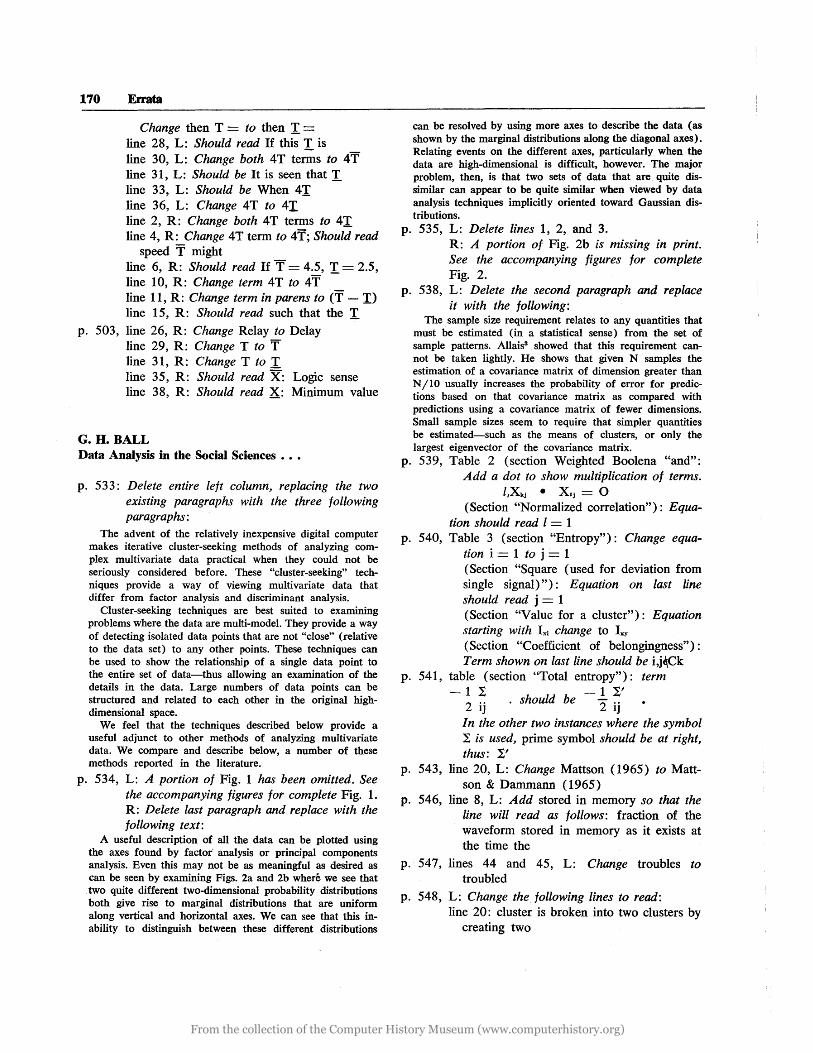
p. 534, L: A portion of Fig. 1 has been omitted. See the accompanying figures for complete Fig. 1. R: Delete last paragraph and replace with the following text:
A useful description of all the data can be plotted using the axes found by factor- analysis or principal components analysis. Even this may not be as meaningful as desired as can be seen by examining Figs. 2a and 2b where we see that two quite different two-dimensional probability distributions both give rise to marginal distributions that are uniform along vertical and horizontal axes. We can see that this inability to distinguish between these different distributions
can be resolved by using more axes to describe the data (as shown by the marginal distributions along the diagonal axes). Relating events on the different axes, particularly when the data are high-dimensional is difficult, however. The major problem, then, is that two sets of data that are. quite dissimilar can appear to be quite similar when viewed by data analysis techniques implicitly oriented toward Gaussian distributions.
p. 535, L: Delete lines 1, 2, and 3. R: A portion of Fig. 2b is missing in print. See the accompanying figures for complete Fig. 2.
p. 538, L: Delete the second paragraph and replace it with the following:
The sample size requirement relates to any quantities that must be estimated (in a statistical sense) from the set of sample patterns. Allais3 showed that this requirement cannot be taken lightly. He shows that given N samples the estimation of a covariance matrix of dimension greater than N /10 usually increases the probability of error for predictions based on that covariance matrix as compared with predictions using a covariance matrix of fewer dimensions. Small sample sizes seem to require that simpler quantities be estimated-such as the means of clusters, or only the largest eigenvector of the covariance matrix.
p. 539, Table 2 (section Weighted Boolena "and": Add a dot to show multiplication of terms.
I,Xkj • Xl j == 0 (Section "Normalized correlation"): Equa-
tion should read I == 1 p. 540, Table 3 (section "Entropy"): Change equa
tion i == 1 to j == 1 (Section "Square (used for deviation from single signal)"): Equation on last line should read j == 1 (Section "Value for a cluster"): Equation starting with Ix! change to Ixy (Section "Coefficient of belongingness"): Term shown on last line should be i,j~Ck
p. 541, table (section "Total entropy"): term - 1 I -1 I'
2 .. . should be -2·· q q In the other two instances where the symbol I is used, prime symbol should be at right, thus: I'
p. 543, line 20, L: Change Mattson (1965) to Mattson & Dammann (1965)
p. 546, line 8, L: Add stored in memory so that the line will read as follows: fraction of the waveform stored in memory as it exists at the time the
p. 547, lines 44 and 45, L: Change troubles to troubled
p. 548, L: Change the following lines to read: line 20: cluster is broken into two clusters by
creating two
From the collection of the Computer History Museum (www.computerhistory.org)

p: 1/4
o
-2.0
o P:1/4
-2.0
- - - -
I
-1.97 I 1
-2' -I'
"- UNIFORM ~ PROBABIliTY
DENSITY. TOTAL PROBABILITY OIF 1/2
- -- -
1.0
-1.0
~--'+1.732
1-1•112 ---
Errata 171
P:1/4
o
2.0
I [-r4 oi~'] 0.6~:[·Ke-Z xlo 1Jx
'A
- -
. "I
--
1.97 \1
"2
. .L
I UNIFORM
PROBABILITY DENSITY. TOTAL PROBABILITY OF 1/2
Fig. 1 THREE DISTRIBUTIONS OF DATA HAVING THE SAME COVARIANCE MATRIX
From the collection of the Computer History Museum (www.computerhistory.org)

172 Errata
THIS NUMBER IS THE PROBABILITY OF A DATA POINT LYING IN THIS SQUARE. THE POINTS ARE UNIFORMLY DISTRIBUTED WITHIN EACH BOX .
• x,
Fig. 2b A UNIFORM, TWO DIMENSIONAL DISTRIBUTION OF POINTS HAVING UNIFORM MARGINAL DISTRIBUTION
line 21: cluster points out of the original cluster. A second
line 22: allowable number of patterns in a cluster, the allowable maximum
p. 550, line 17, L: Change to read: around this by utilizing an arbitrary threshold. All
p. 552, lines 1-8, L: Change to read:
normally distributed so that correlations have the desired significance. It seems quite probable that in cases in which a relatively large number of patterns is being used and in which a priori knowledge is not really adequate to divide these patterns into homogeneous subsets that this will not be true.
line 17, L: Correct spelling of phenomena line 49, R: Change to read tween the technique
of Mattson & Dammann27 and that of Cooper
From the collection of the Computer History Museum (www.computerhistory.org)
line 51, R: Change to read son and Dammann have taken the underlying philosophy of the
p. 553, line 2, L: Should read the Mattson and Dammann technique particularly useful. The most
p. 554, line 38, iR: Alphnumeric should be alphanumeric
p. 555, L: Change the following lines to line 12: distance of all patterns from this aver
age. Set a line 14: from this overall average) where
o L. k. All line 18: allowable cluster size is 1. The overall
average of line 19 L: Add all patterns would be used as
the initial cluster point.
p. 558, line 11, L: Add n to name Dammann.
A. R. HOLMES and R. K. AUSMAN Information Processing of Cancer Chemotherapy Data
p. 583, line 4, L: Change chemotheraphy to chemotherapy
p. 585, line 51, R: Change fransit to transit
p. 586, line 12, L: Change deliquent to delinquent line 1, R: Change Institutes or to Institutes of line 15, R: Change mM1620 to mM 1620
LEHMAN, SENZIG, AND LEE Serial Arithmetic Techniques
p. 716, line 42, R: Change or to of
p. 718, line 4, L: Should read (1 + logsn)·t line 5, L: Delete t
p. 721, line 35, L: Should read bn mt. I
line 37, L: Should read an mi i
line 42, L: Should retid e2-lto
line 43, L: Should read 1 > 181 > 2-t& or
8==0 new line 44, L: Change to 1 > E ~ 0 line 24, R: Change 4 to 5 line 25, R: Change 5 to 6
p. 725, line 3, L: Change 2. __ to 2. M. Lehman
Errata 173
N.V.FINDLER
Human Decision Making •••
p. 738, line 25 and 26, R: Change to Logic Theorist or the General Problem Solver
p. 739, line 19, R: Change to {y} == F( {x}) line 40, R: Change to to this, the concept
p. 741, line 40, R: Change behaps to perhaps p. 743, line 6, L: Change ding on sich to Ding on sich
line 5, R: Change etc.; Hooke to etc., Hooke last line, R: Foot,!;ote omitted:
*One subject, disregarding the fact that there were three independent variables instead of two, considered the environment as some terrain and the £ values representing the height of mountains, hills, and valleys. His "hillclimbing" was a tourist's excursion.
p. 744, line 32, L: Change the one to the ones last lines, L : Footnote not needed line 29, R: Indent to start under "Well
p. 746, line 17, L: Change lowing to lowering p. 748, last line, L, and first line, R: Write last line
of formula as: + 8.sin k 1[. + 10. 8k ,o(mod 1),
4
line 7, R: Change to Y2 == 250 - 200. <Tx2,9 + 20.cos tw +
p. 749, Appendix III: Text sections on left and right-hand sides incorrect relative to each other. Corrected Appendix III is reproduced on next pages.
MAEDA, TAKESmMA, and KOLK
mgh-Speed, Woven Read-Only Memory
p. 800: Figures and text that should appear on this page appear on p. 1034.
MAY, POWELL, and ARMSTRONG
A Thin Magnetic Film Computer Memory •••
p. 804, line 1, R: Should follow line 12
D. E. RIPPY and D. E. HUMPHRIES MAGIC-A Machine for Automatic Graphics •••
p. 820, lines 35-37, R: Change (0 The Z Field specifies (Continued page 180)
From the collection of the Computer History Museum (www.computerhistory.org)
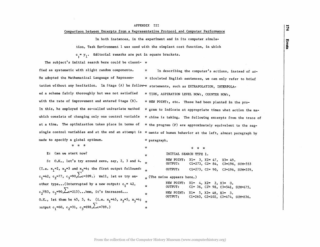
APPENDIX III
Comparison between Excerpts from a Representative Protocol and Computer Performance
In both instances, in the experiment and in its computer simula-
tion, Task Environment 1 was used with the simplest cost function, in which
c;= Yl. Editorial remarks are put in square brackets.
The subject's initial search here could be classi- * fied as systematic with slight random components. -;~ In describing the computer's actions, instead of ar-
He adopted the Mathematical Language of Represen- * ticulated English sentences, we can only refer to brief
tation without any hesitation. In Stage (A) he follow~ statements, such as EXTRAPOLATION, INTERPOLA-
ed a scheme fairly thoroughly but was not satisfied
with the rate of improvement and entered Stage (B).
* TION, ASPIRATION LEVEL NOW:, COUNTER NOW:,
"" NEW POINT:, etc. These had been planted in the pro-
In this, he employed the so-called univariate method * gram to indicate at appropriate times what action the ma-
which consists of changing only one control variable * chine is taking. The following excerpts from the trace of
at a time. The optimization takes place in terms of * the program (p) are approximately equivalent to the seg-
single control variables and at the end an attempt is * ments of human behavior at the left, almost paragraph by
made to specify a global optimum.
* * * E: Can we start now?
S: O.K., let's try around zero, say, 2, 3 and 4.
(I.e. x l =2, x2=3 and x3=4; the first output followed:
c l =42, c2=77, c3=90,L:c=209., Well, let us try an
other type ••• (Interrupted by a new output: c l =
c2V83 , C3=90,L:C=2l5) ••• hmm, it's increased •••
42,
O.K., let them be 45, 5., 4. (Le. x l =45, x2=5, x3=4;
~utput c l =60, c2=3l, c3=698,~C=789.)
* paragraph.
* * * * *
INITIAL SEARCH TYPE 1.
NEW POINT: * OUTPUT:
"le OUTPUT:
Xl= 3, X2= 47, Cl=273, C2= 84,
Cl=273, C2= 90,
X3= 49. C3=196, SUM=553
C3=l96, SUM=559.
* (The noise appears here.)
NEW POINT: Xl= 4, X2= 2, X3= 0. * OUTPUT: Cl= 36, C2= 98, C3=54l, SUM=675.
* NEW POINT: Xl= 5, X2= 48, X3= 3. OUTPUT; Cl=260, C2=102, C3=474, SUM=836.
* *
I~ ~
i
From the collection of the Computer History Museum (www.computerhistory.org)
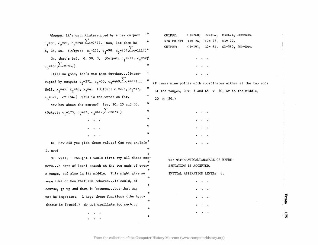
Whoops, it's up ••• (interrupted by a new output: *
Now, let them be ')'( c l =60, c2=29, c3=698,~C=787).
c1=273, c
2=90, c3=754,~C=1117)* 4, 48, 48. (Ou'tput:
Oh, that.' s bad. 0, 50, 0. (Output: c l =271, c2=52~
c3=460,~C=783.) *
Still no good, let's mix them further ••• (inter
rupted by output: c l =27l, c2=50, c3=460,~c=78l) •••
Well, xl=45, x2=48 , x3=4. (Output: c l =278, c2=27,
c3=879, c=1184.) This is the worst so far.
Now how about the center? Say, 20, 25 and 30.
(Output: c l =173, c2=83, C3=6l7,l:C=873.)
,',
'i(
'i(
')'(
')'(
* ~"
'i(
,,(
E: How did you pick these values? Can you explain*
it now7 * * S: Well, I thought I would first try all these cor
* ners ••• a sort of local search at the two ends of every
* x range, and also in its middle. This might give me 'i(
some idea of how that sum behaves ••• It could, of ')'(
course, go up and down in between ••• but that may 'i(
not be important. I hope these functions (the hypo-'i(
thesis is formed!) do not oscillate too much ••• 'i(
i'r
OUTPUT: Cl=260, C2=104, C3=474, SUM=838.
NEW POINT: Xl= 24, X2= 27, X3= 22.
OUTPUT: Cl=19l, C2= 64, C3=589, SUM=844.
(p names nine points with coordinates either at the two ends
of the ranges, ° x 5 and 45 x 50, or in the middle,
20 x 30.)
THE MATHEMATICAL LANGUAGE OF REPRE
SENTATION IS ACCEPTED.
INITIAL ASPIRATION LEVEL: 8.
Ii I~
From the collection of the Computer History Museum (www.computerhistory.org)

S: Now I have ••• how many ••• four, five reasonable ,'r
points. The sums here are no worse than, say, 800. * "k Let us be careful now ••• I want to give you a good Xl •••
It's better if I don't care about these continuous outputs*
now ••• Well, when Xl was around zero, the sum was * about 210; when it was 28, we had almost 600. So, how -I~
about ••• howabout, say, if xlequals 10 ••• that might * hit the minimum ••• This kind of th~ng can give us, shall ,'r
* ,'t
SELECTED SUBSET OF POINTS:
Xl= 3, X2= 47, X3= 49, SUM=553; Xl= 4, X2= 2, X3= 0, SUM=675; Xl= 4, X2= 3, X3= 50, SUM=680; Xl= 46, X2= 4, X3= 1, SUM=779.
(p selects four points out of the nine " . non-no~sy ones,
with the lowest total cost values.)
INTERPOLATION: INTERPOLATION: INTERPOLATION:
Xl=2l; X2=22; X3=25.
(=3+(46-3).553/(553+779) (=2+(47-2).675/(675+553) (=0+(,50-0).675/( 675+680)
NEW POINT: Xl= 21, X2= 22, X3= 25. OUTPUT: Cl=130, C2= 97, C3=563, SUM=780. OUTPUT: Cl=130, C2=103, C3=563, SUMf::786. COUNTER NOW: 1.
we say, 15 for x2' and ••• well ••• I'm doing the same for
x3 ••• O.K., let jt be 20. (Output: c l =134, c 2=108, c3=
736, Lc=778.) It didn't do much good ••• O.K., let us
include this point as well ••••
* (p fails to hit upon a sum better than at least 779, by
* interpolation. It is counting the number of failures.)
,~
,'r
*
*
,'r
,'r
*
,'t
"Ir
,'r
,,,
*
so
SELECTED SUBSET OF POINTS:
Xl= 3, X2= 47, X3= 49, SUM=553; Xl= 4, X2= 2, X3= 0, SUM=675; Xl= 4, X2= ~, X3= 50, SUM=680; Xl= 46, X2= 4, X3= 1, SUM=779; Xl= 21, X2= 22, X3= 25, SUM=780; Xl= 5, X2= 48, X3= 5, SUM=804.
(p selects six points out of the ten "non-noisy" ones far, with'the lowest total cost values.)
,.. I~
Ii
From the collection of the Computer History Museum (www.computerhistory.org)
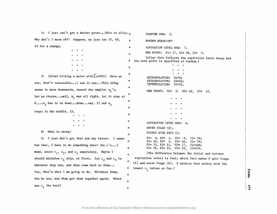
S: I just can't get a better point ••• This is silly.* COUNTER NOW·: 5.
Why don't I move off? Suppose, we just try 35, 40,
45 for a change.
S: (After hitting a point withl:c=58l) Here we
are, that's reasonable ••• I see it now ••• This thing
seems to move downwards, toward the smaller x2's.
Let us choose ••• well, xl was all right, let it stay at
8, ••• x2 has to be down ••• down ••• say, 15 and x3
stays in the middle, 25.
E: What is wrong?
S: I just don't get that sum any better. I some-
how feel, I have to do something about the c's ••• I
mean, about c l ' c2' and c3 separately. Maybe I
should minimize c1 only, at first. Let c2 and c3 be
whatever they are; and then come back to them •••
Yes, that's what I am going to do. Minimize them,
one by one, and then get them together again. Where
was c l the best?
)'r RANDOM BREAK-OUT
* ASPIRATION LEVEL NOW: 7.
* NEW POINT: Xl= 17, X2= 38, X3= 9.
(After five failures the aspiration level drops and * the next point is specified at random.)
,'r
* ,'r
*
* "I(
-k
* -/(
* ,'r
"I(
* ,'r
* * * ,'r
*
EXTRAPOLATION: EXTRAPOLATION: INTERPOLATION:
Xl=O; X2=48; X3=23.
NEW POINT: Xl= 0, X2= 48, X3= 23.
ASPIRATION LEVEL NOW: 4.
ENTER STAGE (B).
POINTS WITH BEST Cl:
Xl= 4, X2= 2, X3= 0, Xl= 45, X2= 4, X3= 46, Xl= 32, X2= 11, uX3= 17, Xl= 21, X2= 22, X3= 25,
Cl= 36; Cl= 59; Cl=106; Cl=130.
(The difference between the inital and current
aspiration levels is four, which fact makes P quit Stage
(A) and enter Stage (B). P selects four points with the
lowest c l values so far.) ~
i =
~ ...... ......
From the collection of the Computer History Museum (www.computerhistory.org)
,'(
-J(
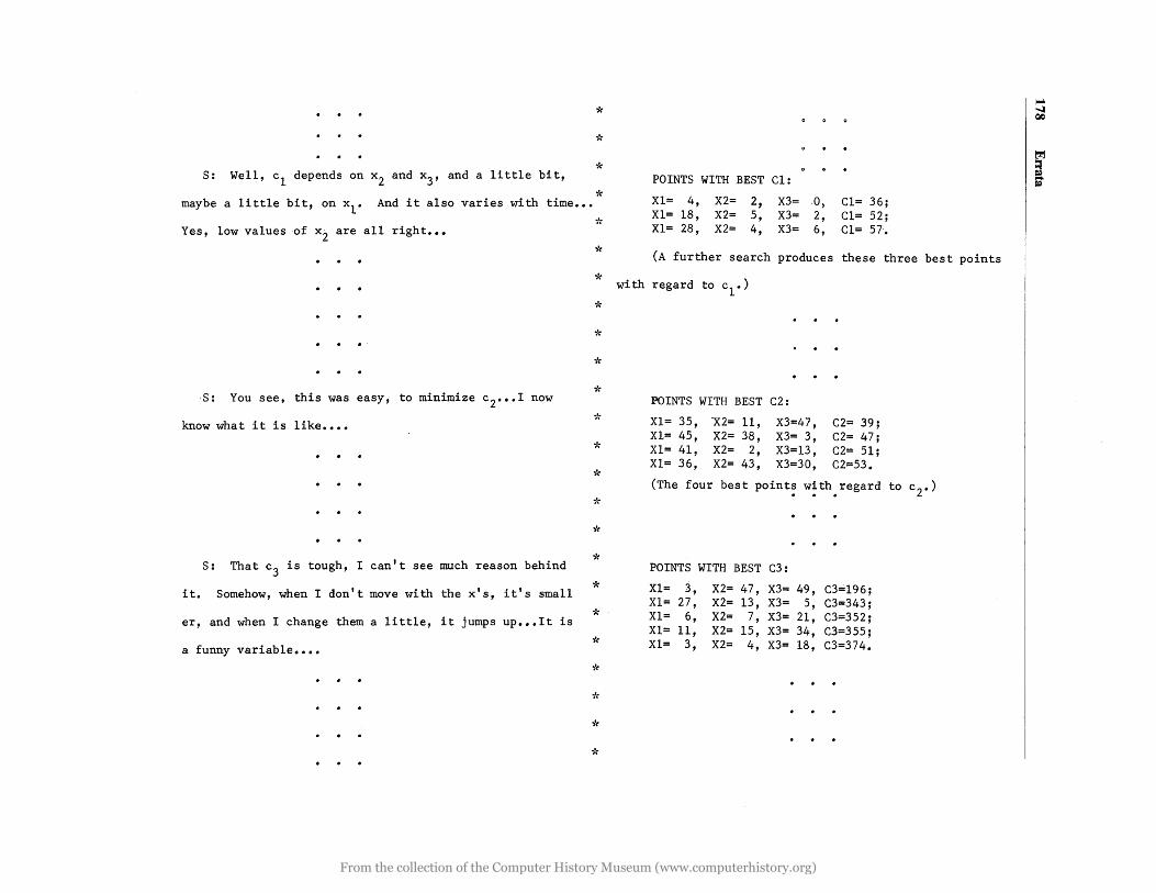
-J( S: Well, c l depends on x2 and x3 ' and a little bit,
* maybe a little bit, on xl. And it also varies with time ••• -/(
Yes, low values of x2 are all right ••• .,~
POINTS WITH BEST Cl:
Xl= 4, X2= 2, X3= 0, Cl= 36; Xl= 18, X2= 5, X3= 2, Cl= 52; Xl= 28, X2= 4, X3= 6, Cl= 57.
(A further search produces these three best points
* with regard to cl.)
S: You see, this was easy, to minimize c 2 ••• I now
know what it is like ••••
S: That c3 is tough, I can't see much reason behind
it. Somehow, when I don't move with the XIS, it's small
er, and when I change them a little, it jumps up ••• It is
a funny variable ••••
.,~
* ,'(
.,'(
.,'(
.,~
~'~
-/(
-/(
* * -;'c
* -/(
.,~
,~
*
POINTS WITH BEST C2:
Xl= 35, ~2= 11, XI= 45, X2= 38, Xl= 41, X2= 2, Xl= 36, X2= 43,
X3=47, X3= 3, X3=13, X3=30,
C2= 39; C2= 47; C2= 51; C2=53.
(The four best points w~th.regard to c 2.)
POINTS WITH BEST C3:
Xl= 3, X2= 47, X3= 49, C3=196; Xl= 27, X2= 13, X3= 5, C3=343; Xl= 6, X2= 7, X3= 21, C3=352; Xl= 11, X2= 15, X3= 34, C3=355; Xl= 3, X2= 4, X3= 18, C3=374.
~ ....... QC
~
i
From the collection of the Computer History Museum (www.computerhistory.org)
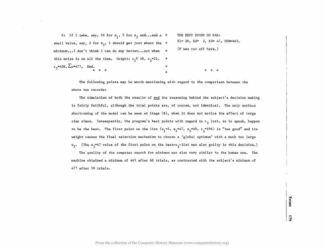
S: If I take, say, .36 for xl' 5 for x 2 and ••• and a
small value, say, 2' for x3 ' I should get just about the
~"
;~
THE BEST POINT SO FAR:
Xl= 28, X2= 2, X3= 47, SUM=463.
minimum ••• I don't think I can do any better ••• not when * (p was cut off here.)
this noise is on all the time. Output: cl~ 48, c2=2l, ,'(
,'( i'( -J(
* ;'( -J( -Ir
c3=408, Lc=477. End. -Jr
The following points may be worth mentioning with regard to the comparison between the
above two records:
The simulation of both the results of and the reasoning behind the subject's decision making
is fairly faithful, although the trial points are, of course, not identical. The only serious
shortcoming of the model can be seen at Stage (B), when it does not notice the effect of large
step sizes. Consequently, the prograII).' s best points wi th regard to c3 just, so to speak, happen
to be the best. The first point on the list (xl=3, x2=47, X3=49 , c
3=l96) is "too good" and its
weight causes the final selection mechanism to choose a 'global optimum' with a much too large
X3• (The x3=47 value of the first point on the best-c2-list was also guilty in this decision.)
The quality of the computer search for minimum was also very similar to the human one. The
machine obtained a minimum of 463 after 68 trials, as contrasted with the subject's minimum of
477 after 59 trials.
~ .. ~ S
i-o& -.J ~
From the collection of the Computer History Museum (www.computerhistory.org)
180 Errata
the display· characteristics for the associated X and Y coordinate fields.
p. 821, Fig. 3, last line: Change (short, med., long) to (solid, dashed)
p. 822, lines 40 & 44, L: Change 1278 to 1778 line 51, L: Change one bit to three bits
p. 824, Table 2: Change left column pair heading to Data List Before Delete
p. 826, line 19, L: Change 1278 to 1778 p. 827, lines 33-36, R: Change first sentence of para
graph to A typical delete subroutine also consists of two machine instructions. Delete remainder of sentence (lines 34-36)
p. 828, line 24, L: Remove s from blocks line 34, L: Add s to instruction line 42, L: Change if to of
p. 830, line 32, L: Change to the same central computer
A.BURNS Hybrid Computer for Lunar Excursion •••
pp. 899-900, Figs. 3 and 4: Figures reversed (captions are correct)
A. P. SAGE and R. W. BURT Optimum Design and Error Analysis • . •
p. 903, line 10, L: Change t to T eq. 3: Change x(T) to x(t)
p. 904, eq. 10: Change y(n-1)T to y(ii=iT); and y'(n - l)T to y'(n - 1 T)
p. 909, eq. 20: Change cosdT to cosbT
N
p. 912, eq. 21: Change I to K=O
eqs. 24 and 25: Should be ~ (nT) == \l yf[Yd (nT),
P] ~y (un T) + R[Ya (nT)-Yd (nT)] (24)
Ap (nT) == \l J[Yd (nT)~ f] ~y-(n + 1 T) + Ap (fiT] T) (25)
line 1, R: Change 6 to \l eq. 29: Change ~i(jT), !(jT) + to <~i(jT),
!(jT»
p. 913, eq. 32: Change n q-H to n q+1
eq. 34: Change nq+1(nT) to nq+l(jT)
M. W. GOLDMAN Design of a High Speed DDA p. 930, line 26, L: pIes equation should be pIer equa
tion line 13, R: ~ should be +
p. 931, line 17, L: very should be vary line 21, R: 1.000 should be 1000
p. 932, line 7, L: d~ should be d (~) line 14, L: convential should be conventional line 16, L: sole should be scale
p. 933, line 15, R: ~ X IT should be ~ X IT p. 934, line 10, L: Replace all symbols u in eq. (1)
with u; Quantity f3r should be under square root sign
line 12, L: Period after range line 1, R: Replace all symbols u in eq. (2)
with u; delete comma and ft following integral
line 2, R: Replace all symbols u in eq. (3) with IT
line 3, R: Replace all symbols u in eq. (4) with IT; minus sign precedes quantity on right side
line 6, R: Replace Ui with IT; p. 935, Replace all symbols u with IT
line 8, L: mixi- should be maxi-line 18, R: Quantity f3r should be under square
root sign Fig. 2: Integrator marked cos t/J in upper
right is integrator 10 p. 936, Replace all symbols u with IT
line 3, L: Quantity f3r should be under square root sign
line 18, L: 1Z should be liZ line 24, R: Quantity x should be under square
root sign p. 937, line 2, L: Ditto
line 5, L: Ditto and x == ~ should be x = (11 2
line 3, L: d 1 should be d~ x
Fig. 3: chapman's in caption should be Chap-man's
p. 938, line 11, L: th should be the p. 941, line 1, R: Quantity ~ should be ~y'
"Registers and adders" should be italicized and spaced as a heading
line 27, L: C = no overflow should be C no overflow
line 30, L: yields should be ~ = yields line 43, L: (C -OUT-) should be (C ==;:;::..
-OUT-) bottom, R: follOWIng tabulation should be
From the collection of the Computer History Museum (www.computerhistory.org)
Top Related