


Languages
Pages
Legal


An Information Theoretic Framework and Self-organizing Agent-based Sensor Network
Architecture for Power Plant Condition Monitoring
Self-Organizing Logic

Agenda
• Introduction • Project Goals • Project Objectives • Technical Approach • Expected Results • Project Elements
– Information Architecture – Virtual Sensors and Sensor Processing – Self-organization – System Integration
• Conclusions
2
Topics and Themes
Agenda
• Element Objectives • Challenges and Opportunities • Technical Approach • Design Study Results
– Swarm Intelligence • Foraging
– Biologically-inspired optimization – General foraging behaviors
• Other eusocial behaviors (sorting, recruitment,….)
• Proposed Framework – Apply to Real Steam Plant Data
3
Topics and Themes

Base System
4
Electric Power System
The operation of a power generation plant must be understood within the context of its environment. Most notably, that it is driving an electric power system with time varying loads and configurations that directly affect the operation of power generation equipment.

Base System
5
Coal-fired Power Generation Plant

Coal-fired Power Plant
• Coal & ash handling – Handles treatment and storage of coal – Handles and dispose of ash
• Steam generating – Creates steam for the greater percentage of power station
in-efficiency • Energy conversion
– Converts steam energy to rotational mechanical energy – Converts rotational mechanical energy into electrical
energy. • Feed water & cooling
– Condenses steam used in boiler chamber back to water for re-use
Key functions
6

Measurement and Sensors
• Pressure measurement – Mechanical instruments (dial gauges) – Electronic pressure transducers
• Flow measurement – Flowrate measurement
• Flowrate / pressure differential devices • Liquid filled manometers
– Electronic differential pressure instrument – Magnetic induction flow measurement – Volumetric flow meters
• Turbine type (widely used for centrifugal pump) • Gear wheel type • Rotary piston type
– Flow indicators
Phenomena and available instrumentation
7

Measurement and Sensors (Cont.)
• Power Measurement – Torque measurement – Torque measurement with eddy current sensors – Electrical power measurement (Current and Voltage
measurement) • Speed measurement
– Mechanical tachometers – Impulse transmitters – Eddy current generators – Slip meters
8
Phenomena and available instrumentation
Measurement and Sensors (Cont.)
• Temperature measurement
– Mechanical contact thermometers – Electrical contact thermometers
• Resistance thermometers • Thermocouples
• Vibration measurement – Accelerometers
9
Phenomena and available instrumentation

Target System
10
Self-organizing, information centric sensor network

Project Goals
1. Enable robust and flexible health and condition monitoring systems through the development of an intelligent agent-based information theoretic architecture for advanced power plant applications.
2. Develop self-organizing computational algorithms that maximize the collection, transmission, aggregation, and conversion of data into actionable information for monitoring, diagnosis, prognosis, and control of the power plant.
3. Demonstrate the viability and efficacy of an agent- based, information-theoretic system for real-time health and condition monitoring of power generation equipment and systems.
11
Realizing the potential of next generation instrumentation systems

Project Objectives
• Develop the theoretical foundations and the algorithms necessary to elicit system structure from available measurements.
• Develop the signal processing, filtering, and inference algorithms and software systems necessary to detect, diagnose, and prognose defects, degradation, and faults in power generation systems at component, subsystem, and system levels.
• Develop algorithms and software systems that enable a sensor network for condition monitoring of power generation plants to be adaptive, resilient, and self-healing.
• Evaluate the effectiveness of these computational algorithms in maximizing information extracted from power plant data and realizing its value for condition monitoring using a power plant simulation test bed. 12
Realizing a sensor network for health and condition monitoring

Technical Approach
• System elements are considered as nodes in a communication network; – Elements send “messages” via physical media to other
system elements, – Elements “process” messages from other elements and
alter their states accordingly. • Instrumentation provides a means for accessing some
of these “messages”; – Messages may be corrupted, – Not all messages can be observed directly.
• Proper understanding of observations requires an understanding of both the processing and the network topology!
13
Systems viewed as communication networks

Information Theory
• Information is the amount of surprise contained in the data; – Data that tells you what you already know is not
informative, – Not all data is created equal.
• The fundamental measure of information is Shannon entropy: where X 2 X is a discrete R.V., X is a finite set known as the alphabet, and .
14
Data and Information are not the same!
H(X) = ¡X
x2X
p(x) logd p(x);
p(x) = PrfX = xg

The Multivariate Case
• For a pair of discrete R.V.’s (X,Y) with joint and conditional distributions p(x,y) and p(x|y), the joint and conditional entropies are, respectively:
• The relationship between these R.V.’s is captured by Mutual Information:
• These quantities are related via the chain rule:
15
The Calculus of Information
H(X; Y ) = ¡X
x2X
X
y2Y
p(x; y) log2 p(x; y)
H(XjY ) = ¡X
x2X
X
y2Y
p(x; y) log2 p(xjy)
I(X; Y ) =X
x2X
X
y2Y
p(x; y) log2
p(x; y)
p(x)p(y)
I(X; Y ) = H(X)¡ H(XjY )

Information Channels
• Let X and Y be the input alphabet and output alphabet, respectively, and let S be the set of channel states. An information channel is a system of probability functions: where , , and for
• Mutual information between the input and output provides a measure of channel transmittance:
• The maximum over all distributions is known as the channel capacity.
16
Modeling Information Flow
pn(¯1; : : : ; ¯nj®1; : : : ; ®n : s)
®1; : : : ; ®n 2 X ¯1; : : : ; ¯n 2 Y s 2 S n = 1; 2; : : : :
T (X ;Y) = H(X ) ¡H(XjY)

Systems and Information
• The properties of information, e.g., its branching property, provide a fundamental basis for decomposing systems.
• The generalization of information theory to N-dimensions provides a statistical analysis tool for understanding systems in terms of the information geometry of its variables; – Permits measurement and analysis of rates of
constraints (i.e., historical conditioning), – System decomposition follows from decomposition of
constraints on information and associated rates.
17
Information Geometry
Information Rates
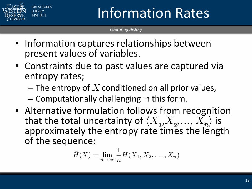
• Information captures relationships between present values of variables.
• Constraints due to past values are captured via entropy rates; – The entropy of X conditioned on all prior values, – Computationally challenging in this form.
• Alternative formulation follows from recognition that the total uncertainty of hX1,X2,…, Xni is approximately the entropy rate times the length of the sequence:
18
Capturing History
¹H(X) = limn!1
1
nH(X1; X2; : : : ; Xn)

Information Structure
• Can determine the communications topology provided by available observation processes; – fusing information from multiple sensors, – Reconstituting lost or degraded sensing, – Detect system changes reflected in changing
communication topology. • Identify “correlative” structure of sensor data;
– Provides means of identifying relevant (possibly abstract) subsystems,
– Basis for mesoscopic models and “summary” variables.
19
Systems as Communication Networks

System Structure
• System § is defined as a set of ordered variables where the set of internal variables is denoted §int and directly observable variables by §out
20
Information-theoretic View of Systems
§ = fXij1 · i · ng

System Decomposition
• Systems are characterized by their associated variables hence information theoretic measures can be applied, e.g.,
• Information chain rules provide a calculus for partitioning systems,
• More sophisticated “Laws of Information” can be constructed.
21
Systems and Chain Rules
H(§) = ¡X
s2S
p(s) log2 p(s);
¹I(§i; §j) = ¹H(§i) + ¹H(§j)¡ ¹H(§i; §j)
Expected Results
• Effective (accurate, computationally tractable with sufficient precision) means of computing entropy measures for the processes/components/systems of interest.
• Distributed and self-organizing method for using entropy measures to identify intrinsic structure of power generation systems.
• Self-organizing method for combining observations with dynamics/behaviors/events of interest.
• Statistical techniques for detecting/classifying/identifying conditions of interest and characterizing the severity and prognosis of system performance degradation.
22
Fundamental building blocks for self-organizing sensor network for condition monitoring
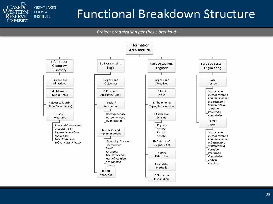
Functional Breakdown Structure
23
Project organization per thesis breakout

Self-Organizing Logic

Element Objectives
• Develop algorithms and software systems that enable a sensor network for condition monitoring of power generation plants to be adaptive, resilient, and self-healing. – Develop techniques, algorithms, and software for
dynamically discovering the intrinsic communication topology of power generation systems.
– Develop techniques, algorithms, and software for associating sensor data streams with operational objectives.
– Develop techniques, algorithms, and software for reconstituting lost or degraded sensing and communication capabilities.
25

Challenges and Opportunities
• Scaling problems associated with centralized methods: – Complexity, – Transmission of large amounts of data to central processes
(bandwidth, QoS), – Computational footprint (cycles, memory).
• Accommodate existing infrastructure • Lack of detailed a priori understanding of components, processes,
and their interactions • Wide variation in operating conditions, system permeability • Ubiquitous computational and (wireless) communication resources • Power management technologies engendering a new class of
instrumentation” – No umbilical – Physically reconfigurable on-the-fly
26
Chal
leng
es
Opp
ortu
nitie
s

Technical Approach
• The aforementioned constraints and opportunities mandate a distributed, and agent-based approach and strongly suggest the use of biologically inspired algorithms.
• Distributed – Monolithic approaches do not scale well and tend to be “brittle,” i.e. do not accommodate
new instrumentation or permit reorganizing existing infrastructure without significant rework.
• Agent Based – Agent based approaches are flexible and embed inherent system descriptions. They provide a
powerful basis for bottom-up application to complex systems and minimize communication requirements while distributing processing tasks in a realistic manner.
• Biologically Inspired – Biologically inspired approaches provide the machinery necessary to capture emergent
phenomena and thus provide a basis for accommodating unanticipated contingencies. This is crucial for large-scale complex systems where all contingencies cannot be enumerated.
27

Sensor Network
28
Connecting data to operational needs and objectives
• Discovering the actual topology of the system’s intrinsic communication structure.
• Associating information streams with monitoring processes.
• Extracting the information from the relevant data streams for fault detection, diagnosis and prognosis.

Topology Discovery
• The first step in implementing the sensor network is to determine the system’s intrinsic topology. The intrinsic communication between elements of the system manifests in the mutual information between the sensing performed at disparate locations of the network and thus can be used to extract the system’s intrinsic topology.
• Biologically inspired approaches are strong candidates for developing the distributed agent based system for the sensor network.
29
Overview of Swarm Intelligence
• In particular, Swarm Intelligence is investigated for these purposes: – Swarm intelligence is inspired by the collective behavior of animals in nature.
Some natural examples include insect colonies, bird flocks, and fish schools. – A swarm intelligence system consists of a group of agents interacting locally
with each other and with their environment. The agents follow simple rules governing their local behaviors that, in turn emerge global behaviors in a bottom-up fashion.

Principles of Swarm Intelligence
1. Self-organization – Positive Feedback (Amplification) – Negative Feedback (Balancing) – Amplification of Fluctuations (Random Walks, Error) – Multiple Interactions
2. Stigmergy Indirect communications between system elements via
interaction with environment, i.e. individual behavior modifies the environment which in turn modifies the behavior of other individuals
3. Bounded Autonomy Local behaviors are not specified in a deterministic
manner, rather bounds on allowable behaviors are given, typically probabilistically.
30
Candidate Approaches
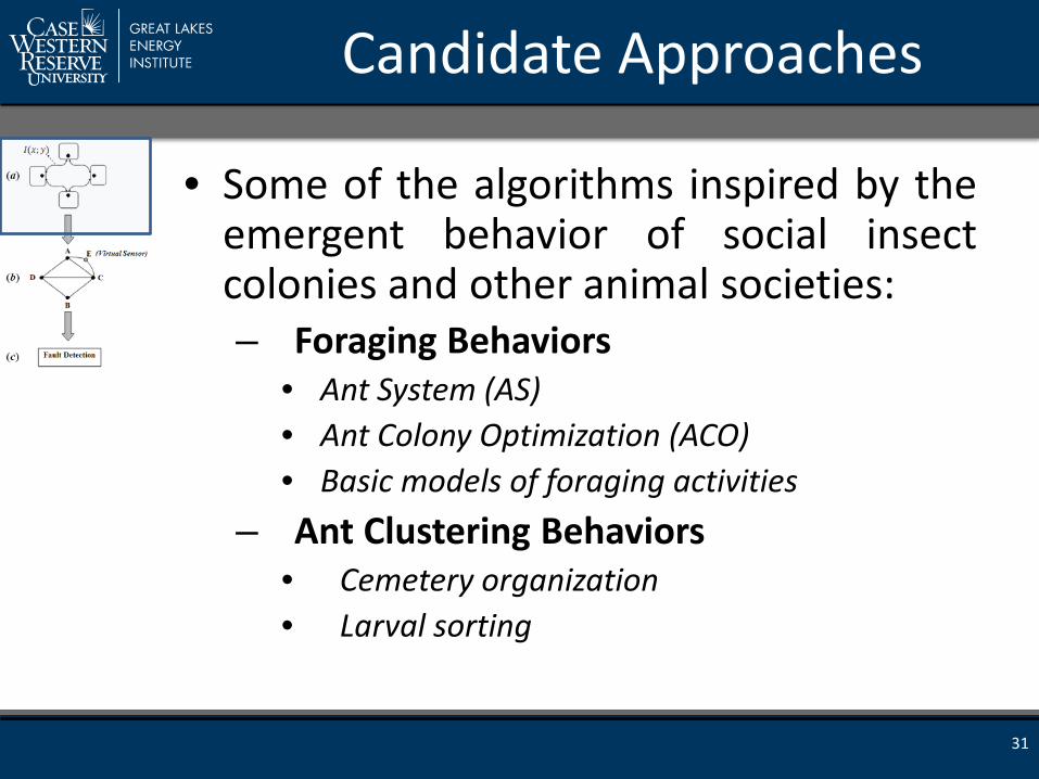
• Some of the algorithms inspired by the emergent behavior of social insect colonies and other animal societies: – Foraging Behaviors
• Ant System (AS) • Ant Colony Optimization (ACO) • Basic models of foraging activities
– Ant Clustering Behaviors • Cemetery organization • Larval sorting
31

Foraging Behavior
32
Foraging Patterns of Three Army Ant Species with Different Diets
These behaviors are used as a basis for optimization approaches due to its tendency to find the shortest path, most notably Ant System and Ant Colony Optimization. Further, the behaviors can be adapted to the specifics of the problem at hand.
• Eciton hamatum • Diet: dispersed social
insect colonies • Food distribution: rare
but large
• Eciton rapax • Diet: intermediate diet • Food distribution:
intermediate food source
• Eciton burchelli • Diet: scattered arthropods • Food distribution: can
easily be found but each time in small quantities
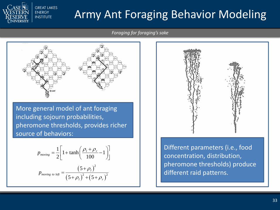
More general model of ant foraging including sojourn probabilities, pheromone thresholds, provides richer source of behaviors:
Army Ant Foraging Behavior Modeling
33
Foraging for foraging’s sake
Different parameters (i.e., food concentration, distribution, pheromone thresholds) produce different raid patterns.
1 1 tanh 12 100
l rmovingp ρ ρ + = + −
( )( ) ( )
2
2 2
5
5 5l
moving to leftl r
pρ
ρ ρ
+=
+ + +

Optimization in Foraging Behavior
34
An introduction to Ant Colony Optimization (ACO)
• Introduced by Marco Dorigo (1992) • Ants lay a pheromone trail as they move. Pheromone levels
increase with traffic but decrease with dissipation over time. The pheromone marking is thus reinforced on frequently used trails are and fades on infrequently used trails.
• Two ants start with equal probabilities of taking either path. shorter path => shorter transit time => more pheromone => the next ant takes the shorter path
• The combination of reinforcing pheromone trail leads to the shortest path to the food source. With random search procedures, the ants tend to also explore the alterative food sources.

ACO/AS Simulation
• Applied AS and ACO to problem of finding shortest paths on a network – System elements and sensors => nodes – Find shortest information distance => greatest
mutual information • Three networks considered:
– Different number of nodes, – Different configurations.
• Implemented in Matlab©
• Examined performance and tuning options
35
Network detection as optimization problem

Networks
36
The three considered networks
Network 1 29 Nodes
Network 2 38 Nodes
Network 3 194 Nodes
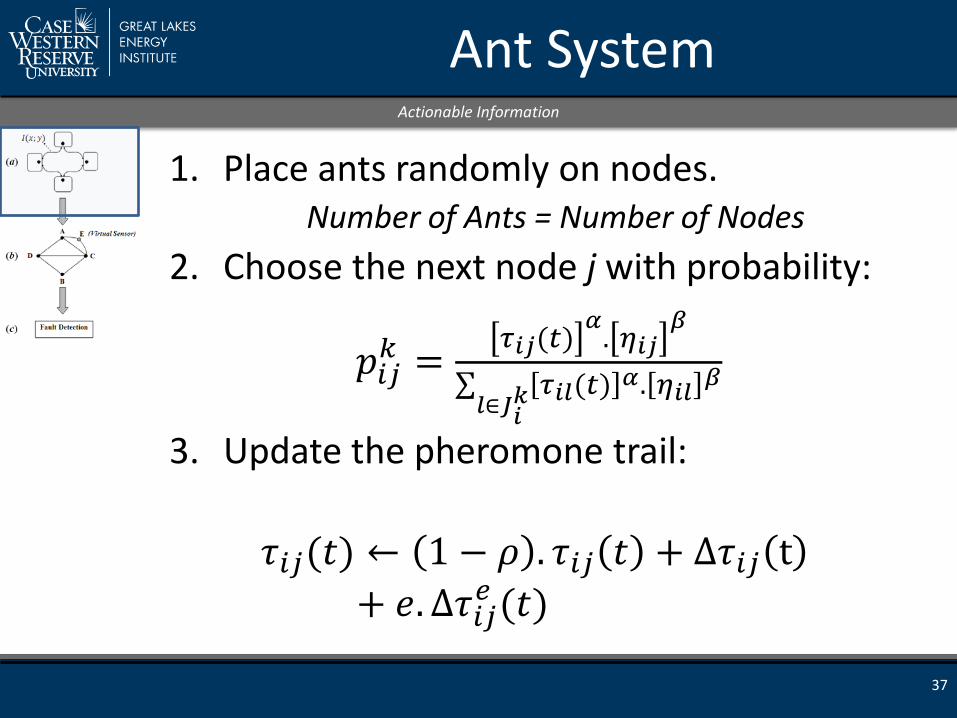
Ant System
1. Place ants randomly on nodes. Number of Ants = Number of Nodes
2. Choose the next node j with probability:
𝑝𝑝𝑖𝑖𝑖𝑖𝑘𝑘 = 𝜏𝜏𝑖𝑖𝑖𝑖(𝑡𝑡) 𝛼𝛼. 𝜂𝜂𝑖𝑖𝑖𝑖𝛽𝛽
∑ 𝜏𝜏𝑖𝑖𝑖𝑖(𝑡𝑡) 𝛼𝛼. 𝜂𝜂𝑖𝑖𝑖𝑖 𝛽𝛽𝑖𝑖∈𝐽𝐽𝑖𝑖𝑘𝑘
3. Update the pheromone trail:
𝜏𝜏𝑖𝑖𝑖𝑖(𝑡𝑡) ← 1 − 𝜌𝜌 . 𝜏𝜏𝑖𝑖𝑖𝑖 𝑡𝑡 + ∆𝜏𝜏𝑖𝑖𝑖𝑖 t+ 𝑒𝑒.∆𝜏𝜏𝑖𝑖𝑖𝑖𝑒𝑒 (𝑡𝑡)
37
Actionable Information

Results
Network Iterations Accuracy
Network1 25 % 89.12
Network 2 25 % 98.35
Network 3 25 % 77.34
38
Comparing the algorithm accuracy for each network
Network 1 29 Nodes
Network 2 38 Nodes
Network 3 194 Nodes

Observations
• The AS algorithm performance does not scale well with increasing node count.
• Displays poor sensitivity to adjustable parameters (i.e. not easily tuned).
39
Ant Colony System
• Ant Colony System is similar to Ant System, which is based on the foraging behavior of ants.
• There are four main differences between these two algorithms: I. Exploration II. Transition Rule III. Global Trail Update IV. Local Trail Update
40

Results
Network Number of Agents Number of Iterations Accuracy
Network1
50 25 % 98.5
100 50 % 95.8
Network 2
50 25 % 100
100 20 % 100
Network 3 200 50 % 82.8
300 25 % 81.9
41
Comparing the algorithm accuracy for each network
Network 1 29 Nodes
Network 2 38 Nodes
Network 3 194 Nodes
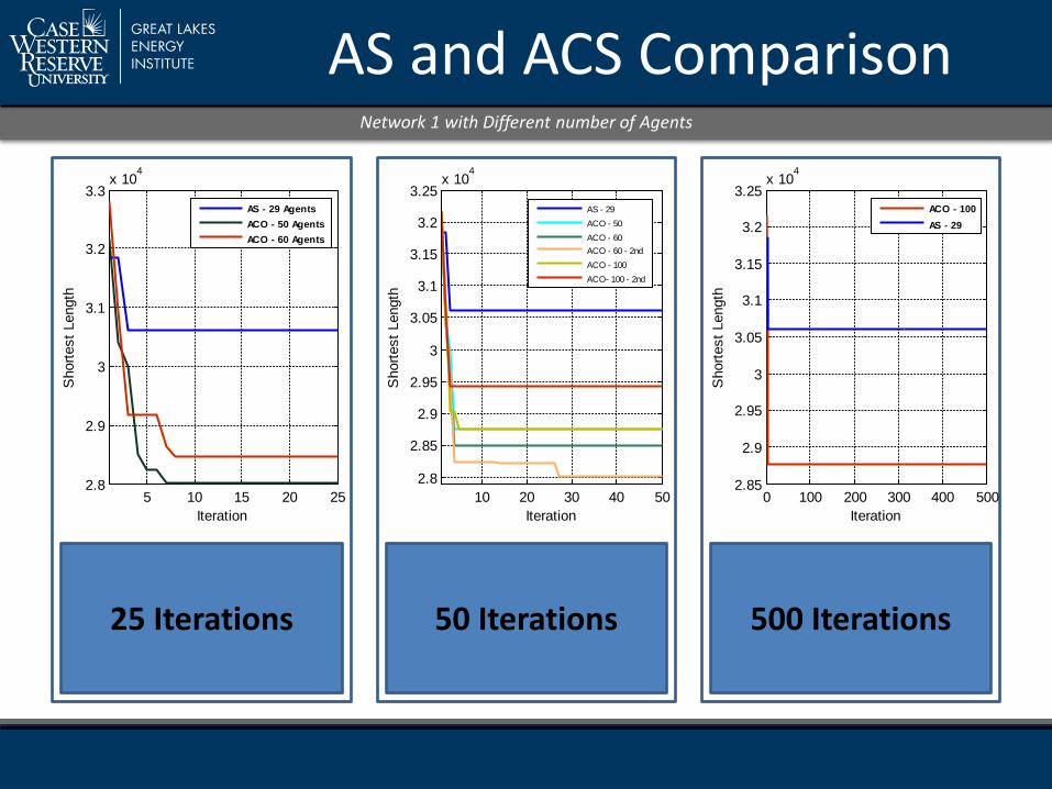
AS and ACS Comparison
25 Iterations 50 Iterations 500 Iterations
Network 1 with Different number of Agents
5 10 15 20 252.8
2.9
3
3.1
3.2
3.3x 10
4
Iteration
Sho
rtest
Len
gth
AS - 29 AgentsACO - 50 AgentsACO - 60 Agents
10 20 30 40 502.8
2.85
2.9
2.95
3
3.05
3.1
3.15
3.2
3.25x 10
4
Iteration
Sho
rtest
Len
gth
AS - 29ACO - 50ACO - 60ACO - 60 - 2ndACO - 100ACO- 100 - 2nd
0 100 200 300 400 5002.85
2.9
2.95
3
3.05
3.1
3.15
3.2
3.25x 10
4
Iteration
Sho
rtest
Len
gth
ACO - 100AS - 29

AS and ACS Comparison
• Network 3 • 25 Iterations
Networks 2 and 3 with Different number of Agents
• Network 2 • 25 Iterations
5 10 15 20 25
6660
6680
6700
6720
6740
6760
6780
Iteration
Sho
rtest
Len
gth
AS - 38
ACO- 50
5 10 15 20 251.09
1.1
1.11
1.12
1.13
1.14
1.15
1.16
1.17
1.18x 10
4
Iteration
Sho
rtest
Len
gth
AS - 194
ACO - 200ACO - 30

Recapitulation
• The ACS algorithm works better than the AS algorithm.
• Changing the characteristics of the algorithm such as parameter values will not affect the results.
• The selection of the starting points at each iteration and pheromone trail update play an important role in this algorithm. Choosing the appropriate strategy will improve the results.
• These methods are designed for optimization and are limited in the behaviors that they can demonstrate and hence the flexibility that they offer.
44
ACO and AS Comparison

Steam Plant Simulation
The Reference Unit: − Alstom’s ultra-supercritical pulverized coal-fired plant design − Gross electrical output of 1080MWe. − The steam generator will produce steam flow to a turbine
generator with boiler outlet conditions of main steam flow of 600°C @ 278 bar g and RH outlet steam flow of 605°C @ 58 bar g.
− The plant net heat rate is 9045 kJ/kWh. Model Subsystems: − steam generator (boiler) − steam turbines − feedwater preheating system
45
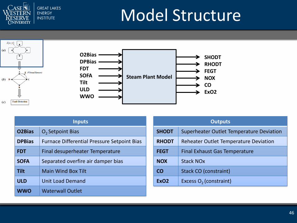
Model Structure
Inputs
O2Bias O2 Setpoint Bias
DPBias Furnace Differential Pressure Setpoint Bias
FDT Final desuperheater Temperature
SOFA Separated overfire air damper bias
Tilt Main Wind Box Tilt
ULD Unit Load Demand
WWO Waterwall Outlet
Outputs
SHODT Superheater Outlet Temperature Deviation
RHODT Reheater Outlet Temperature Deviation
FEGT Final Exhaust Gas Temperature
NOX Stack NOx
CO Stack CO (constraint)
ExO2 Excess O2 (constraint)
Steam Plant Model
O2Bias DPBias FDT SOFA Tilt ULD WWO
SHODT RHODT FEGT NOX CO ExO2
46
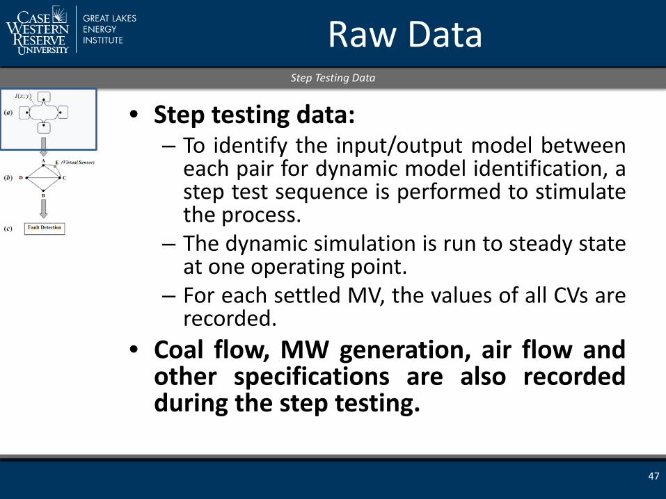
Raw Data
• Step testing data: – To identify the input/output model between
each pair for dynamic model identification, a step test sequence is performed to stimulate the process.
– The dynamic simulation is run to steady state at one operating point.
– For each settled MV, the values of all CVs are recorded.
• Coal flow, MW generation, air flow and other specifications are also recorded during the step testing.
47
Step Testing Data

Step Test for O2Bias
48
Normalized
-0.1
0.1
0.3
0.5
0.7
0.9
1.1
19-Dec-12 07:59:31 19-Dec-12 09:11:31
O2Bias
SHODT
RHODT
FEGT
NOX
CO
ExO2

Preparing Data for Modeling
• Normalize data between [0.1]. – Normalization does not impact correlation
coefficient calculations. • Construct IDDATA object for used with
Matlab’s System Identification Toolbox. • Construct model:
– Merge all data sets into a single data set and compute a MIMO model.
• Results were not promising. The single model could not capture the nonlinearity between all of the input/output pairs.
– A SISO model is computed for each input/output pair. At the end we will have 6x7 SISO models for our steam plant simulation.
49
System Identification

SISO Modeling Results
• Hammerstein-Wiener Model – Block Diagram :
• w(t) = f(u(t)): nonlinear function transforming input
data u(t). • x(t) = (B/F)w(t): linear transfer function. • y(t) = h(x(t)): nonlinear function that maps the
output of the linear block to the system output.
50
System Identification
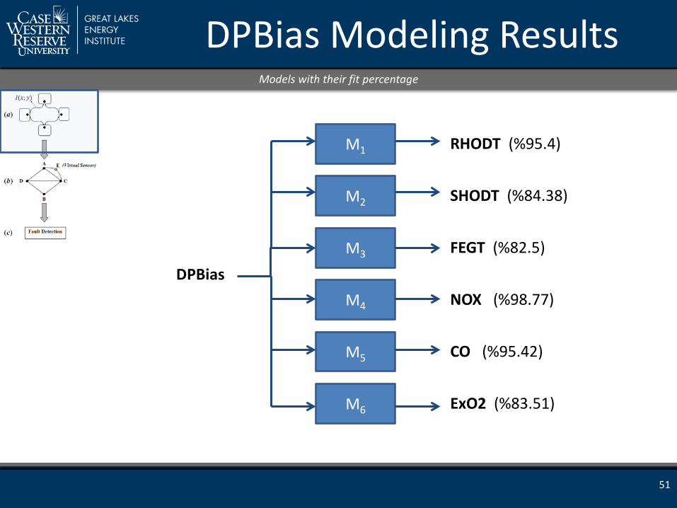
DPBias Modeling Results
51
Models with their fit percentage
M1
M2
M3
M4
M5
M6
DPBias
RHODT (%95.4)
SHODT (%84.38)
FEGT (%82.5)
NOX (%98.77)
CO (%95.42)
ExO2 (%83.51)
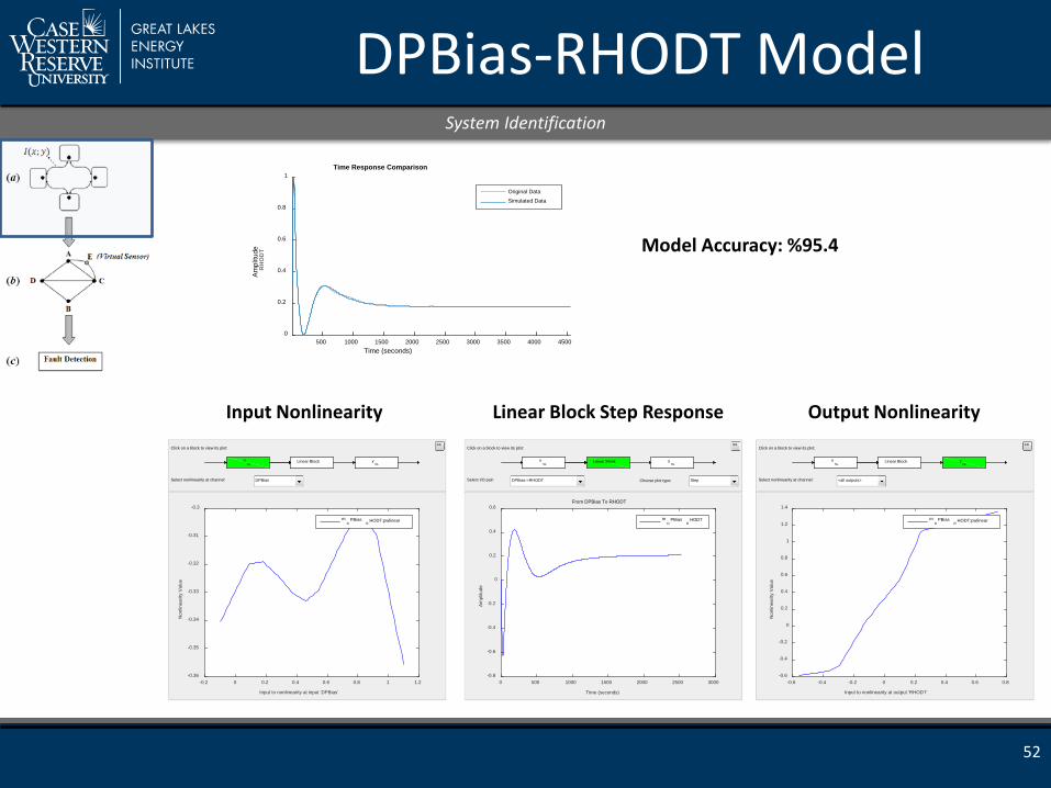
DPBias-RHODT Model
52
System Identification
yNL
Linear BlockuNL
Click on a block to view its plot:
Select nonlinearity at channel: DPBias
Input to nonlinearity at input 'DPBias'
-0.2 0 0.2 0.4 0.6 0.8 1 1.2
Non
linea
rity
Val
ue
-0.36
-0.35
-0.34
-0.33
-0.32
-0.31
-0.3
mD
PBiasR
HODT:pwlinear
>>
yNL
Linear BlockuNL
Click on a block to view its plot:
Select I/O pair: DPBias->RHODT Choose plot type: Step
Time (seconds)
0 500 1000 1500 2000 2500 3000
Am
plitu
de
-0.8
-0.6
-0.4
-0.2
0
0.2
0.4
0.6From DPBias To RHODT
mD
PBiasR
HODT
>>
yNL
Linear BlockuNL
Click on a block to view its plot:
Select nonlinearity at channel: <all outputs>
Input to nonlinearity at output 'RHODT'
-0.6 -0.4 -0.2 0 0.2 0.4 0.6 0.8
Non
linea
rity
Val
ue
-0.6
-0.4
-0.2
0
0.2
0.4
0.6
0.8
1
1.2
1.4
mD
PBiasR
HODT:pwlinear
>>
Time Response Comparison
Time (seconds)
Am
plitu
de
500 1000 1500 2000 2500 3000 3500 4000 45000
0.2
0.4
0.6
0.8
1
RH
OD
T
Original DataSimulated Data
Model Accuracy: %95.4
Input Nonlinearity Output Nonlinearity Linear Block Step Response
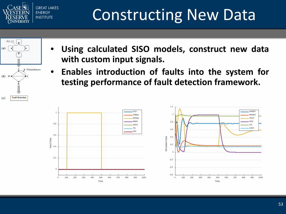
Constructing New Data
• Using calculated SISO models, construct new data with custom input signals.
• Enables introduction of faults into the system for testing performance of fault detection framework.
53
Time
0 100 200 300 400 500 600 700 800 900 1000
Inpu
t Dat
a
0
0.2
0.4
0.6
0.8
1 ULD
O2Bias
DPBias
WWO
SOFA
Tilt
FDT
Time
0 100 200 300 400 500 600 700 800 900 1000
Sim
ulat
ed D
ata
-0.6
-0.4
-0.2
0
0.2
0.4
0.6
0.8
1
1.2
SHODT
RHODT
FEGT
NOX
CO
ExO2

Network Discovery The observation of physical system from a foraging perspective
Agent going from node 6 to node 2: Behavior:
The agent carries the data, w6 ,from its home node to the next node.
Food Definition: The Correlation Coefficient between the time series w6 and w2.
xi : a time series which is the observations at node I wi : a time series which is the partial observations of xi at node i
2
6
1 2x
6x4x
3
4 5
1x 3x
5x
6w
2w
7 u
54

Proposed Algorithm Based on Foraging Behavior of Ants
• A set of agents are randomly placed on the nodes such that each node has at least one agents.
• Agents select the next node based on the current correlation coefficient for that time frame. They favor the nodes with higher correlation coefficient.
• As the agents travel, pheromone is deposited on the edges as a function of correlation coefficient between the source and destination node.
• Based on the pheromone values at the end of the last iteration, a topology is extracted.
55

Proposed Algorithm Based on Foraging Behavior of Ants
• For agent 𝒌𝒌 at node 𝒊𝒊, the next node 𝒋𝒋 is chosen based on the following rule:
– 𝑞𝑞 : a random variable uniformly
distributed over – 𝑞𝑞0: a tunable parameter over – : set of all the nodes in the system
except for the current node – : node that is randomly selected
according to this probability:
𝑝𝑝𝑖𝑖𝑖𝑖𝑘𝑘 (𝑡𝑡) =𝑔𝑔(𝑤𝑤𝑖𝑖 ,𝑤𝑤𝑖𝑖)(𝑡𝑡)
∑ 𝑔𝑔(𝑤𝑤𝑖𝑖 ,𝑤𝑤𝑖𝑖)(𝑡𝑡)𝑙𝑙∈𝑖𝑖𝑖𝑖𝑘𝑘
• The agent 𝒊𝒊 goes to node 𝒋𝒋 and updates the pheromone trail of the pair (𝒊𝒊, 𝒋𝒋) according to the following rule: where:
– Note that the exact value of correlation coefficient is deposited on the edge which is different from the previous version.
0
0
g ( , ) _ ( , )
arg max { g ( , ) } q q
q q
ki
i u i u
i uu J
w w correlation coefficient w w
w w ifj
J if∈
=
≤= >
kiJ
kiJ J∈
( ) (1 ) ( ) ( , )ij ij i jt t f w wτ ρ τ← − ⋅ +
( , ) _ ( , )i j i jf w w correlation coefficient w w=
56

Initialization
• Number of Nodes= 7 • Number of Agents= 7x100
– 7 distinct swarms, each containing 100 agents, deployed to the network at different times during the simulation. Each swarm deposits a distinct pheromone and only follow their own pheromone on the edges.
• Time Period=50s • Initial Value on pheromone Trail=0 • pheromone decay coefficient=0.1 • Initial position of the agents= random,
but at least one agent at each node
57

Simulation Snapshot
58
Time (seconds)
0 100 200 300 400 500 600 700 800 900 1000
Dat
a
-0.5
0
0.5
1
1.5Input/Output Data for DPBias Step Test
SHODT
RHODT
FEGT
NOX
CO
ExO2
Input
Discovered Topology

Information/Objective Mapping
• Having the knowledge on intrinsic topology, we can properly align our observation processes, including virtual sensors, with the intrinsic communication topology.
• Virtual sensors can be used to: 1. Sense things that we cannot
directly instrument. 2. Validate or verify other
measurements. 3. Reconstitute lost sensing and
communication.
59

Graph Similarity Measures
• Graph similarity techniques can be used to detect the changes in the extracted topology.
• These changes can be the result of a fault in the system or the changes in system’s dynamics.
• In a class of similarity methods in which an element (e.g., a node or edge) in graph GA and an element in graph GB are considered similar if their respective neighborhoods within GA and GB are similar.
60

Pattern Mining
• In pattern mining, dynamic graphs have been analyzed from two main research tracks: – The study of the properties that describe
the topology of the graph, – The extraction of specific sub-graphs to
describe the graph evolution.
61

Fault Detection and Diagnosis
• Map the information streams to operational objectives and needs for fault detection.
62
Processing the information/objective mapping for Fault Detection
Conclusions
• In this presentation, we discussed foraging behavior and raid patterns of army ants.
• Examined and run simulation for two optimization algorithms based on social behavior of ants.
• Proposed a new algorithm for condition monitoring of a steam plant based on foraging behavior of ants and applied it to real data.
• For the path forward, we will explore graph similarity and pattern mining techniques to select the appropriate approach for our project.
63

64
Thank you…

BACKUP SLIDES
65

DIFFERENCES BETWEEN ACS AND AS ALGORITHMS
66

1- Exploration
• A Candidate List is formed for each city which is the list of preferred cities to be visited from that given city and consists of cl closest cities. – From any given city, first the candidate list for that
city is examined for possible next city. – If all the candidate list cities are visited, the next
city will be the closest of the yet unvisited cities.

2- Transition Rule
• An ant k on city i chooses the next city j to move based on the following rule:
𝑗𝑗 = �arg𝑚𝑚𝑚𝑚𝑚𝑚𝑢𝑢∈𝑖𝑖𝑖𝑖𝑘𝑘 𝜏𝜏𝑖𝑖𝑢𝑢(𝑡𝑡) . 𝜂𝜂𝑖𝑖𝑢𝑢 𝛽𝛽 𝑖𝑖𝑖𝑖 𝑞𝑞 ≤ 𝑞𝑞0
𝐽𝐽 𝑖𝑖𝑖𝑖 𝑞𝑞 > 𝑞𝑞0
– q: a random variable uniformly distributed over [0,1] – q0: tunable parameter over [0,1] – 𝐽𝐽 ∈ 𝐽𝐽𝑖𝑖𝑘𝑘 : city that is randomly selected according to this
probability:
𝑝𝑝𝑖𝑖𝑖𝑖𝑘𝑘 (𝑡𝑡) =𝜏𝜏𝑖𝑖𝑖𝑖(𝑡𝑡) . 𝜂𝜂𝑖𝑖𝑖𝑖
𝛽𝛽
∑ 𝜏𝜏𝑖𝑖𝑙𝑙(𝑡𝑡) . 𝜂𝜂𝑖𝑖𝑙𝑙 𝛽𝛽𝑙𝑙∈𝑖𝑖𝑖𝑖𝑘𝑘
3- Global Trail Update
• The global trail updating is only applied to the edges belonging to the best tour since the beginning of the trial:
𝜏𝜏𝑖𝑖𝑢𝑢 𝑡𝑡 ← 1 − 𝜌𝜌 . 𝜏𝜏𝑖𝑖𝑢𝑢 𝑡𝑡 + 𝜌𝜌.∆𝜏𝜏𝑖𝑖𝑢𝑢(𝑡𝑡)
– (𝑖𝑖, 𝑗𝑗): the edges belonging to the best tour 𝑇𝑇+ – 𝜌𝜌: a parameter governing the pheromone decay – ∆𝜏𝜏𝑖𝑖𝑢𝑢 𝑡𝑡 = 1
𝐿𝐿+⁄

4- Local Trail Update
• The local pheromone update is performed after each transition by the following formula:
𝜏𝜏𝑖𝑖𝑢𝑢 𝑡𝑡 ← 1 − 𝜌𝜌 . 𝜏𝜏𝑖𝑖𝑢𝑢 𝑡𝑡 + 𝜌𝜌. 𝜏𝜏0
– 𝜏𝜏0 = (𝑛𝑛. 𝐿𝐿𝑛𝑛𝑛𝑛)−1: the initial value of pheromone trail – 𝑛𝑛: number of cities – 𝐿𝐿𝑛𝑛𝑛𝑛: length of a tour produced by the nearest neighbor
heuristic

DETAILED RESULTS FOR ACS
71

Network 1 Simulation Results
Number of Agents Number of Iterations Accuracy
50 25 % 98.5
50 50 % 95.8
60 25 % 96.9
60 50 % 96.7
100 50 % 95.8
100 500 % 95.8
500 5 % 84.3
72
Comparing the algorithm accuracy for network 1
0 10 20 30 40 502.8
2.85
2.9
2.95
3
3.05
3.1
3.15
x 104
Iteration
Shor
test
Len
gth
100 Agents - 50 Iterations100 Agents - 500 Iterations100 Agents - 50 Iterations - 2nd500 Agents - 5 Iterations50 Agents - 25 Iterations50 Agents - 50 Iterations60 Agents - 25 Iterations60 Agents - 50 Iterations60 Agents - 50 Iterations - 2nd
Network 1 with 29 Nodes
0 0.1 0.2 0.3 0.4 0.5 0.6 0.7 0.8 0.9 10
0.1
0.2
0.3
0.4
0.5
0.6
0.7
0.8
0.9
1

Network 2 Simulation Results
Number of Agents Number of Iterations Accuracy
50 25 % 100
60 20 % 100
100 20 % 100
73
Comparing the algorithm accuracy for network 2
Network 2 with 38 Nodes
5 10 15 20 256650
6700
6750
6800
Iteration
Shor
test
Len
gth
50 Agents - 25 Iterations60 Agents - 20 Iterations100 Agents - 20 Iterations
0 0.1 0.2 0.3 0.4 0.5 0.6 0.7 0.8 0.9 10
0.1
0.2
0.3
0.4
0.5
0.6
0.7
0.8
0.9
1

Network 3 Simulation Results
Number of Agents Number of Iterations Accuracy
200 25 % 82.8
300 25 % 81.9
200 50 % 82.2
74
Comparing the algorithm accuracy for network 3
Network 3 with 194 Nodes
5 10 15 20 25 30 35 40 45 501.095
1.1
1.105
1.11
1.115
1.12
1.125
1.13
1.135x 10
4
Iteration
Shor
test
Len
gth
200 Agents - 25 Iterations300 Agents - 25 Iterations200 Agents - 50 Iterations
0 0.1 0.2 0.3 0.4 0.5 0.6 0.7 0.8 0.9 10
0.1
0.2
0.3
0.4
0.5
0.6
0.7
0.8
0.9
1

CORRELATION COEFFICIENT AND NORMALIZATION
75

Correlation Coefficient Normalization Impact
, 2 2
[( )( )]cov(X,Y)[( ) ] [( ) ]
min( ) 1,max( ) min( ) max( ) min(X)
min( ) 1,max( ) min( ) max( ) min( )
1 1cov(X,Y)max( ) min(X) max( ) min( )
X YX Y
X Y X Y
new newX X
new newY Y
new
E X YE X E Y
X XXX X X
Y YYY Y Y Y
X Y Y
µ µρσ σ µ µ
σ σ
σ σ
− −= =
− −
−= =
− −
−= =
− −
= − −
, ,
cov(X,Y)
newX Y X Yρ ρ
→ =
Top Related