


Languages
Pages
Legal

AN INVESTIGATION INTO OFDM AS A
SUITABLE MODULATION TECHNIQUE FOR
AN ACOUSTIC UNDERWATER MODEM
by
Johannes du Preez
Thesis presented in partial fulfilment of the requirements for the degree of
Master of Science in Engineering at Stellenbosch University
Supervisor: Dr Riaan Wolhuter
Faculty of Engineering
Department of Electrical and Electronic Engineering
December 2012

i
DECLARATION
By submitting this thesis electronically, I declare that the entirety of the work contained therein is my
own, original work, that I am the sole author thereof (save to the extent explicitly otherwise stated), that
reproduction and publication thereof by the University of Stellenbosch will not infringe any third party
rights and that I have not previously in its entirety or in part submitted it for obtaining any qualification.
December 201ς
Ȣ
Ȣ
Ȣ
Ȣ
Ȣ
Ȣ
Ȣ
Ȣ
Ȣ
#ÏÐÒÙÒÉÇÈÔȢ΄ȢςπρςȢ3ÔÅÌÌÅÎÂÏÓÃÈȢ5ÎÉÖÅÒÓÉÔÙ
!ÌÌȢÒÉÇÈÔÓȢÒÅÓÅÒÖÅÄ
Stellenbosch University http://scholar.sun.ac.za

ii
ABSTRACT
This thesis investigates orthogonal frequency division multiplexing (OFDM) as a viable modulation
technique for an ultrasonic acoustic underwater modem. The underwater environment provides a
challenging setting for acoustic communications. Long delay spreads due to multipath propagation,
severe Doppler frequency shifts, frequency dependent absorption and very limited bandwidth are but
some of the challenges to overcome. OFDM essentially provides the parallel transmission of symbols in
the frequency domain by simultaneously modulating many closely spaced orthogonal subcarriers. The
resulting long parallel symbol rate together with the cyclic extension of symbols render the signal robust
against intersymbol interference (ISI) caused by multipath propagation. Intercarrier interference (ICI)
between the overlapping frequency responses of subcarriers is mitigated by their property of
orthogonality. Doppler spread contributes to the loss of orthogonality and can result in severe ICI. A
method of measuring the Doppler shift by means of including a preamble and postamble symbol with
each data frame is proposed. The detected frequency offset is corrected by resampling the frame at the
desired sample rate. Not only do the ambles serve as a mechanism for timing and frequency
synchronisation, but they are also applied in the channel estimation process. The equalisation of channel
response is required for the coherent demodulation of the received symbols. An investigation into
different phase shift keying (PSK) and quadrature amplitude modulation (QAM) constellations reveal
optimal arrangements for minimal symbol errors. The optimised QAM constellations do not lend
themselves to Gray-coding, so that an efficient interleaving scheme is needed to mitigate the non-uniform
distribution of bit errors among symbol errors. Forward error correction is provided via a Bose
Chaudhuri Hocquenghem (BCH) block code. Variable code rates, together with the ability to switch
between different constellations, enable the modem to perform so-called variable modulation in an
attempt to maximise the throughput under specific channel conditions. The modulation/demodulation
scheme is wholly defined in software as to provide flexibility and facilitate experimentation with different
signal processing methods. The accompanying hardware platform allows for the transmission of a pre-
generated signal and the recording of a received signal for off-line processing. The prototype design
serves as a proof of concept and thus provides only simplex communication. Field tests over limited
distances demonstrate the successful operation of the prototype modem. We conclude that OFDM is
indeed a suitable modulation technique for acoustic underwater communication.
Stellenbosch University http://scholar.sun.ac.za
iii
OPSOMMING
Hierdie tesis ondersoek die toepassing van ortogonale frekwensiedeling multipleksering (OFDM) as
modulasie tegniek op ʼn onderwater kommunikasie modem. Die onderwater omgewing bied vele
uitdagings vir akoestiese kommunikasie. Lang vertraging-verstrooiings as gevolg van multipad
voortplanting, Doppler frekwensieskuif, frekwensieafhanklike absorpsie, en beperkte bandwydte is van
die uitdagings wat oorkom moet word. In essensie bied OFDM die parallelle versending van ʼn aantal
simbole deur die gelyktydige modulasie van verskeie nou-gespasieerde subdraers in die
frekwensiegebied. Die gevolglike lang parallelle simboolperiodes, tesame met die sikliese uitbreiding van
simbole, verleen immuniteit teen intersimbool steurnisse (ISI) wat ontstaan as gevolg van multipad
voortplanting. Die ortogonaliteit van naburige draers in die frekwensiegebied beperk interdraer steuring
(ICI) tussen hul oorvleuelende frekwensie weergawes. Doppler frekwensieskuif kan egter lei tot die
verlies aan ortogonaliteit en bydra tot ernstige interdraer steurings. ʼn Metode wat gebruik maak van
aanhef en slot simbole, ingesluit by elke raam, word voorgestel om die Dopplerskuif te meet. Die bepaalde
frekwensieafset word gekorrigeer deur die monstertempo van die raam aan te pas na die verlangde
tempo. Buiten die tyd- en frekwensie-sinkronisasie funksies van die aanhef en slot simbole, speel dit ook
ʼn belangrike rol in die ontrekking van die frekwensie weergawe van die kanaal. Die effening van die
kanaal se frekwensieweergawe is noodsaaklik vir die koherente demodulasie van die ontvangde simbole.
ʼn Ondersoek na verskillende fase verskuif sleuteling (PSK) en kwadratuur amplitude modulasie (QAM)
konstellasies het optimale rangskikkings opgelewer vir minimale simboolfoute. Hierdie optimale QAM
konstellasies verleen hulself egter nie na Gray-kodering nie. ʼn Effektiewe invlegtegniek is nodig om die
nie-uniforme verspreiding van bisfoute tussen simboolfoute te beperk. Fout korrigering funksionaliteit
word gebied deur ʼn Bose Chaudhuri Hocquenghem (BCH) blokkode. Verstelbare koderingstempo’s en die
vermoë om tussen verskillende konstellasies te skakel, stel die modem in staat om sogenaamde
verstelbare modulasie te gebruik in ʼn poging om die data deurset te optimeer onder spesifieke kanaal
kondisies. Die modulasie en demodulasie skema is volledig in sagteware gedefinieer. Dit verleen
buigbaarheid en vergemaklik eksperimentering met verskeie seinverwerkingstegnieke. Die meegaande
hardeware platvorm stel die modem in staat om vooraf opgewekte seine uit te saai en rou ontvangde
siene op te neem vir na-tydse verwerking. Die prototipe ontwerp dien as ʼn konseptuele bewys en bied
dus slegs simplekse kommunikasie. Die suksesvolle werking van die modem is gedemonstreer deur
toetsing oor beperkte afstande. Hieruit word afgelei dat OFDM inderdaad geskik is vir akoestiese
onderwater kommunikasie.
Stellenbosch University http://scholar.sun.ac.za

iv
TABLE OF CONTENTS
1 Introduction 1
1.1 The Relevance of Underwater Communication 1
1.2 Why Use Acoustic Communication 2
1.3 The Basics of Acoustic Communication 3
1.4 Objectives and Scope of This Project 4
1.5 Overview of Contents 5
1.6 Conclusion 8
2 The Underwater Acoustic Channel 9
2.1 The Speed of Sound in Water 9
2.1.1 Sound Velocity Equation 9
2.1.2 Sound Velocity Profile 10
2.2 Sound Propagation Paths 11
2.2.1 Naturally Occurring Wave Guides 11
2.2.2 Scattering 13
2.3 The Underwater Environment as a Communication Channel 14
2.3.1 Multipath Propagation 14
2.3.2 Doppler Effect 15
2.3.3 Coherence Bandwidth and Coherence Time 16
2.3.4 Propagation Loss 18
2.3.5 Ambient Noise 21
2.4 Summary 22
3 OFDM: The Modulation Scheme of Choice 23
3.1 Orthogonal Multicarrier Modulation 23
3.1.1 Concept of Multicarrier Modulation 23
3.1.2 Multicarrier Modulation from a Signal Processing Perspective 24
3.1.3 Orthogonal Signal Space 27
3.2 Orthogonal Frequency Division Multiplexing 28
3.2.1 OFDM Modulation by Fast Fourier Transform 29
3.2.2 Guard Intervals 30
3.2.3 Time Synchronisation 31
3.2.4 Frequency Synchronisation 31
3.2.5 Spectral Shaping 32
3.2.6 Peak-to-Average Power Ratio 33
3.2.7 Sensitivity to Non-linearities 35
3.3 Applying OFDM to the Underwater Environment 36
3.3.1 Pass Band Modulation 36
3.3.2 Timing and Frequency Synchronisation 38
Stellenbosch University http://scholar.sun.ac.za
v
3.3.3 Channel Estimation 43
3.3.4 QAM Constellations 45
3.3.5 Symbol Error Probabilities 48
3.3.6 Bit Error Probabilities 52
3.3.7 Forward Error Correction and Interleaving 55
3.3.8 Quantisation Resolution 61
3.4 Summary 63
4 Generating and Demodulating the Signal 64
4.1 Signal Parameters 64
4.1.1 Occupied Bandwidth 64
4.1.2 Sampling Frequency 64
4.1.3 FFT window size 65
4.1.4 Number of Words per Frame 65
4.1.5 Frame Structure 65
4.1.6 Declaration of Signal Parameters 66
4.2 Message Parameters 66
4.3 Modulation Process 67
4.4 Demodulation Process 72
4.5 Summary 78
5 Transmitter and Receiver Hardware 79
5.1 Transducers 79
5.1.1 The Workings of Transducers 79
5.1.2 The Characteristics of Transducers 80
5.1.3 Characterisation of Furuno 520-5PSD Transducers 87
5.2 Link Budget 96
5.2.1 Theory of Acoustic Link Budget 96
5.2.2 Link Budget Over 1 km 98
5.3 Electronic Hardware of the Transmitter 99
5.3.1 USB-SPI Converter 100
5.3.2 PIC32MX Buffer 101
5.3.3 Digital-to-analogue Converter and Reconstruction Filter 101
5.3.4 Power Amplifier 102
5.4 Electronic Hardware of the Receiver 104
5.4.1 Variable Gain Low-noise Amplifier 104
5.4.2 Anti-Aliasing Filter and Analogue-to-Digital Converter 105
5.4.3 PIC32MX Buffer 106
5.4.4 USB-SPI Interface 106
5.5 Summary 106
6 Practical Tests and System Evaluation 107
6.1 Objectives of Testing 107
Stellenbosch University http://scholar.sun.ac.za

vi
6.1.1 Hardware Verification 107
6.1.2 Accuracy of Amble Extraction 107
6.1.3 Accuracy of Channel Estimation 108
6.1.4 Link Quality and Error Control Performance 108
6.2 The Test Setup and Conditions 108
6.3 Results 110
6.3.1 Hardware Verification 110
6.3.2 Accuracy of Amble Extraction 111
6.3.3 Accuracy of Channel Estimation 114
6.3.4 Link Quality and Error Control Performance 118
6.4 Conclusion 119
7 Conclusion and Future Work 120
7.1 Future Work 120
References 122
Stellenbosch University http://scholar.sun.ac.za

1
1 INTRODUCTION
Upon mentioning underwater communication to the layman, one is often met with the idea of two scuba
divers frantically trying to warn each other of an approaching shark with misunderstood hand gestures.
Hopefully after reading this thesis, Tom, Dick and Harry will realise that there is more to underwater
communication than just handwaving.
1.1 The Relevance of Underwater Communication
Roughly two thirds of the earth’s surface is covered with oceans, yet when comparing the time and
resources spent on oceanic research with space exploration, the former is dwarfed by organisations such
as NASA with billion dollar budgets. With an ever increasing concern about global warming, rising ocean
temperatures and natural disasters it makes sense to divert our gaze from the heavens and look down
into our own backyard. A better understanding of our oceans and the effect of mankind’s unjudgmatic
dealings with it might prove invaluable for generations to come.
Numerous applications exist for underwater communication. Distributed undersea sensor networks
gather data about ocean currents, water temperature and salinity. This data provides valuable insight into
changing global climate conditions. By monitoring marine life numbers and migrations we are able to
study the effects of overexploitation of marine resources. By observing pollution levels we can control the
dumping of toxic waste in the ocean. In order to interpret the gathered data, these sensing applications
need to transfer the information to a host where it can be processed and analysed.
The National Oceanic and Atmospheric Administration (NOAA) of America have a buoy system in place
that provides real-time tsunami report data. The Deep-ocean Assessment and Reporting of Tsunamis
(DART) system consists of an anchored seafloor pressure recorder and a companion surface buoy for
real-time communications [1]. An acoustic link is used to transmit pressure readings from the seafloor to
the surface buoy which in turn relays the information via satellite to the tsunami warning centre. When
an event is detected a warning is issued to advise possibly affected countries. There are 39 buoys world-
wide, located in high-risk zones.
Remotely operated undersea vehicles are used for exploring deep waters, wreckages, harbours and even
territories under the ice caps. They are often also used for maintenance of ships, oilrigs and deepwater
mining equipment and also for search and retrieve missions. As the name implies these vehicles require
commands from a remote location. An operator can control the movement and orientation and other
functions of the vehicle and typically also have a visual feed of the environment.
Even scuba divers are limited to hand signals and writing slates underwater without some other channel
of communication. While sound propagates well underwater, the human vocal cords are not adapted to
produce sounds in water. In some situations divers need to perform intricate tasks where hand signals or
Stellenbosch University http://scholar.sun.ac.za

1. Introduction
2
writing is simply not practical. Think of divers performing reparations on subsurface equipment with
engineers standing by to assist them from the surface. How else would they communicate other than to
resort to some technological device?
From the above mentioned applications it is clear that a need very well exists to exchange information in
an underwater setting. Although technologies for terrestrial communications are highly developed, these
cannot always be effectively applied to the underwater environment. In the next section we will see how
the shortcomings of conventional terrestrial communication can be overcome by using an acoustic
medium to transmit signals.
1.2 Why Use Acoustic Communication
Not unlike outer space and maybe even more so, the underwater environment is a hostile place for
sensitive scientific equipment. One has to deal with high water pressures and very low temperatures,
especially when venturing into deeper waters. Not to mention the mechanical forces exerted by rough
ocean conditions and water currents. For gathering data from such equipment or providing control
commands to it, one needs to establish a means of communication. Any such communication link would
have to deal with the inherit conditions of the underwater environment.
To provide this link there needs to be a channel made up of some physical medium along which the signal
will propagate. In general terms this channel can be an electrical signal conducted by copper wire,
electromagnetic radio waves or even light waves guided by optic fibre. While all of these technologies are
highly developed, none of them provide a truly ideal solution for underwater communication. Radio
waves are greatly attenuated by water and while they provide a wireless link it will not be effective for
distances of more than a few metres. Copper and optic fibre cable can provide very high data rates over
long distances but will always remain tethered thus severely limiting the mobility of any system.
Another, much more viable option than the above mentioned methods, is acoustic communication. This
uses acoustic pressure waves to carry the information and the water itself as a medium to transport the
signal. Depending on the application, acoustic communication can provide reasonable data rates over
fairly long distances with the advantage that it provides a wireless link between transmitter and receiver
and it does not require line-of-sight operation. Table 1.1 shows the attenuation coefficients of different
wave types and frequencies in salt water [2].
Stellenbosch University http://scholar.sun.ac.za

1. Introduction
3
Wave type Frequency Attenuation constant [dB/m]
Acoustic waves 100 Hz
Acoustic waves 5 kHz
Acoustic waves 30 kHz
Radio waves 100 Hz 0.35
Radio waves 20 kHz 4.9
Radio waves 100 kHz 10
Visible light 600 THz
Table 1.1: The attenuation coefficients of various wave types in salt water.
1.3 The Basics of Acoustic Communication
To gain a better understanding of what is expected of an underwater modem it is valuable to define what
makes up a basic communication link. All communications originate as a message that needs to be
transferred from a source, along a channel, to a destination. The message is in the form of raw digital data
when it enters the transmission path. The transmitter is firstly tasked with encoding this message to
provide resilience against bit errors which may result from distortion of the received signal. The encoding
process usually entails interleaving of the message bits and encoding via a forward error correction code.
The next step is to use the encoded message to generate a signal that can be efficiently transmitted across
the channel. Depending of the modulation scheme used either the amplitude, phase and/or frequency of
the carrier signal is altered as a function of the message. The modulated carrier signal is then amplified
and fed to a transducer. The transducer will convert the electrical energy into mechanical pressure waves
that can propagate along the watery medium.
The carrier signal now travels through the channel where it can experience several different types of
distortion. Distortion will be used as a collective term for a number of impairments that a signal can
suffer. In the underwater environment this includes
delay spreads due to multipath propagation,
Doppler frequency shifts,
frequency dependent absorption
scattering and diffusion
geometrical attenuation due to spreading and
additive ambient noise.
The signal can also be distorted by nonlinearities in the signal path. This includes phenomenon such as
cross-over distortion, clipping and slew rate distortion when the signal is momentarily defined only by
the amplifier characteristics and not the signal waveform itself. If the nature of a distortion is known in
advance the signal can be pre-emphasised before transmission in such a way that in negates the effect of
the distortion. An amount of additive noise also contributes to the loss of quality of the signal.
Stellenbosch University http://scholar.sun.ac.za

1. Introduction
4
At the receiver, a transducer coverts the propagating pressure wave into an electrical signal. During
demodulation it is common to find an estimate of the distortion that the signal undergoes in order to
compensate for it, but some uncertainty remains. An estimate of the encoded message data is extracted by
evaluating the carrier signal according to the specifications of the modulation scheme. The estimated
message data is deinterleaved and decoded by the forward error correction code to correct any residual
errors. Once decoded, the original message can be reconstructed as intended for the destination.
1.4 Objectives and Scope of This Project
The underwater channel presents significant challenges to overcome if an efficient communication link is
to be established. The intention of this study is to formulate a feasible design and implement a prototype
acoustic underwater modem that can meet these challenges. To achieve this, we endeavour to
gain sufficient knowledge of the underwater channel in order to assess the viability of a proposed
modulation scheme,
become acquainted with the intricacies of orthogonal frequency division multiplexing (OFDM)
modulation and evaluate it as a suitable solution for underwater communication,
adapt conventional OFDM as the modulation scheme of choice to better cope with the properties
of the underwater channel,
design, implement and verify by software simulation the efficiency of the proposed modulation
scheme,
design, build and verify a modular hardware platform for testing the modulation scheme,
integrate the software defined modulation scheme and hardware platform to function as a
complete communication system and
verify and evaluate the performance of the complete system by means of field tests.
These objectives give a broad overview of what is to be accomplished with this project. To acts as
guidelines in the design process, we also lay down some physical specifications and requirements of the
modem. The prototype modem should be able to
successfully transmit and receive signals over a range of 1 km,
provide an effective data rate of 20 kbps,
provide adequate reliability through error control techniques and
successfully deal with Doppler frequency shifts up to a ratio of .
The modem serves as a proof-of-concept and its purpose is only to demonstrate the success with which
OFDM can be applied to the underwater environment. For this reason it is adequate that the modem only
provides simplex communication and that the signal processing is performed off-line on a personal
computer.
Stellenbosch University http://scholar.sun.ac.za
1. Introduction
5
1.5 Overview of Contents
This study starts off with an investigation of the acoustic underwater channel. The characteristics of
sound propagation in water will influence the design decisions of the communication link. Some aspects
of the underwater environment are unique, while others apply to communication channels in general.
The critical aspects to be investigated are identified as: the speed of sound in water, the anticipated
severity of Doppler frequency shifts, frequency dependant absorption, scattering and diffusion of sound
waves, multipath propagation, geometric attenuation and ambient noise. A detailed discussion of the
acoustic underwater channel can be found in Chapter 2.
The modulation scheme of choice should be robust against the underwater channel conditions. OFDM is
identified as the most suitable modulation technique. An OFDM signal is made up of a number of digitally
modulated orthogonal subcarriers at closely spaced frequencies. The amplitude and phase of each carrier
is modulated by a symbol from a quadrature amplitude modulation (QAM) constellation. OFDM
essentially transmits multiple QAM symbols simultaneously so that the parallel symbol rate is
considerably lower when compared to single carrier systems with the same transmission rate. This holds
significant advantages for channels that suffer from severe delay spreads due to multipath propagation.
All of the signal processing for OFDM modulation can be performed in the frequency domain. The signal is
generated by assigning QAM symbols to selected carriers in a Fast Fourier Transform (FFT) window. Any
frequency dependent pre-emphasis can simply be applied directly to the FFT window, without the need
for complex filter designs. The signal is converted to the time domain with the Inverse Fast Fourier
Transform (IFFT). The intricacies of the OFDM modulation scheme are explained in Chapter 3.
Carriers are modulated using symbols from QAM constellations. Each symbol represents a certain bit
sequence. The more symbols in a constellation, the higher the resulting data rate. Commonly found
constellations are binary phase shift keying (BPSK), quadrature phase shift keying (QPSK), 16-QAM, 64-
QAM and so forth. These are popular, because its symbols can be organised into a symmetrical
arrangement. This allows for a systematic decoding of the bit sequence. It also lends itself to Gray-coding;
a system that assigns bit sequences to symbols so that a symbol, erroneously decoded as any adjacent
symbol, causes only a single bit error. 16-QAM and higher order constellations are however not all
optimally arranged to provide the lowest symbol error rates for a given signal-to-noise ratio (SNR). Also,
the required improvement in SNR to yield the same symbol error rate between QPSK and 16QAM is much
larger than that between BPSK and QPSK. In an environment where even the smallest performance gain is
valued, it is worthwhile to define an 8-QAM constellation to fill the void between QPSK and 16-QAM and
to optimise all constellations to yield the lowest possible symbol error rates. Details of these
optimisations and an investigation of a suitable forward error correction (FEC) code can be found in
Chapter 3.
Since the transmitter and receiver may move relatively to each other during transmission, the resulting
change in distance between them may cause a Doppler frequency shift. This brings about a change in the
carrier frequencies observed by the receiver. The underwater channel can introduce severe Doppler
Stellenbosch University http://scholar.sun.ac.za

1. Introduction
6
shifts, especially in mobile applications. Consider that the speed of sound in water is approximately
1500 m/s. A remote underwater vehicle (RUV) travelling at 10 km/h or 2.778 m/s will encounter a
Doppler frequency shift with a ratio of . This equates to a frequency shift of 92.3 Hz for a
carrier of 50 kHz. The typical carrier spacing for acoustic underwater OFDM applications is in the order of
hundreds of hertz. It is clear that a Doppler shift of 92.3 Hz will cause severe loss of orthogonality of the
carriers. A method of using preambles and postambles to determine the amount of Doppler shift is
proposed and a resampling technique for correcting it is discussed in Chapter 4. Other parameters of the
generated signal such as the FFT window size, duration of cyclic extension, frame length and so forth are
also examined.
The next step was to design and build the hardware for the modem. The most important design decision
was the choice of transducer. The ideal transducer would have a bandwidth of 20 kHz to provide
sufficient data rates and a transmit voltage response as flat as possible over the frequency band of
interest. Furthermore, the lower the operating frequency of the system, the less the signal will suffer from
frequency dependant absorption thus extending its range for a given transmitter power. A lower
operating frequency also allows for a slower sample rate and means that less computing power is needed
for the modulation and demodulation processes. Unfortunately, a limited budget did not allow the
acquisition of transducers with these ideal characteristics. Instead, two available Furuno 520-5PSD
transducers used for fish finding and depth measurement was used. These devices have resonant
frequencies at 50 kHz and 200 kHz and very narrow bandwidth. It is designed for narrowband pinging
and is not ideal for wideband communications. Characterising the transducers revealed its equivalent
circuit model and with corresponding pre-emphasis, sufficient bandwidth could be achieved to meet the
required data rate. The investigation into transducer characteristics can be found in Chapter 5.
OFDM signals suffer from a high Peak-to-Average Power Ratio (PAPR). This means that the signal
contains high power peaks even though the average power is relatively low. This complicates amplifier
design as it requires a very wide dynamic range to cope with the peak power and still provide sufficient
average power. Techniques using randomisation of the input bit sequences have achieved some success
in controlling the peak amplitudes [3], but these are cumbersome. Others suggest simply clipping the
peaks if the resulting non-linear distortion is tolerable [3]. The underwater environment demands high
data rates over a very narrow bandwidth and introducing unnecessary noise into the communication link
will lower the achievable data rate. The ideal amplifier has a wide dynamic range not to clip the signal
peaks and can provide sufficient slew rate to reach these peaks without excessive non-linear distortion of
the signal. Details on the amplifier design can be found in Chapter 5.
As the acoustic pressure wave travels through the water it will encounter certain gains and losses due to
transducer gain, geometric attenuation and absorption to name a few. A link budget accounts all gains
and losses that a signal may encounter along the transmission path. From the link budget we can calculate
the required receiver sensitivity and transmit power necessary to cover the distance between transmitter
and receiver. The link budget is calculated in Chapter 5.
Stellenbosch University http://scholar.sun.ac.za
1. Introduction
7
When the acoustic pressure wave reaches the receiver it has suffered severe attenuation. In order to
recover the signal it has to be amplified before processing. The amount of required gain can be
determined from the link budget. The receiver is comprised of a low noise, variable gain amplifier that is
connected to an analogue-to-digital converter, via an anti-aliasing filter. The complete design of the
receiver can be found in Chapter 5.
The OFDM signal, with a bandwidth of 20 kHz centred at 50 kHz, requires a Nyquist sample rate of
120 kHz to be discretised accurately. Simulations of the Doppler compensation technique shows that the
resampling process produces improved results at higher sample rates. The sample rate was set at
450 kHz. For digital processing the signal samples also need to be quantised. Quantisation introduces an
error into each sample resulting in so-called quantisation noise. The magnitude of the quantisation noise
can be limited by improving the resolution of the quantisation process. The signal-to-quantisation noise
ratio for a given sample resolution for an OFDM signal is determined in Chapter 4. The availability of high-
resolution analogue-to-digital converters and digital-to-analogue converters imposes no real boundary
on the sample resolution. It will be limited only by the data rate that the system can process. The sample
resolution was set at 16 bits.
Since all signal processing is performed in Matlab, it is necessary to transfer the signal between a
computer and the transmitter/receiver in real-time. At 16 bits per sample, this results in a 7.2 Mbps data
stream. To playback and record the signals requires the design of specialized hardware that can maintain
this transfer rate. A direct Universal Serial Bus (USB) to Serial Peripheral Interface (SPI) link is used to
achieve this. It can provide data rates up to 30 Mbps. Details on the design of the data link and the
accompanying software and hardware can be found in Chapter 5.
Now that the software defined modulation scheme and the physical hardware have been designed and
implemented it can be integrated into a functional system. The signal to be transmitted is generated by a
Matlab script according to the modulation parameters set by the user. The signal is stored the computer’s
hard drive. Upon transmission it is transferred to the playback buffer via the USB-SPI interface. The buffer
temporarily holds the sample values before outputting it to the digital-to-analogue converter at 450 kHz.
The power amplifier drives the transducer that converts the electrical signal into an acoustic pressure
wave. At the receiver the transducer generates an electric signal from the pressure waves encountered.
The signal is amplified and sampled at 450 kHz. Sample values are temporarily stored in the recording
buffer before it is transferred the computer’s hard drive via the USB-SPI interface. The recorded signal is
demodulated by a Matlab script during post-processing.
In order to evaluate the performance of the functional system a series of field tests were conducted in the
large wave flume at the Stellenbosch Council for Scientific and Industrial Research (CSIR) facilities. The
dimensions of the flume are 100 m x 3 m x 1 m. Regrettably the full length could not be utilised. The
movement of the trolley over the flume was limited and it could only be positioned 62 m away from the
far end. Using the back wall of the flume as a reflective surface the signal could be transmitted over an
effective distance of 124 m. The elongated nature of the water body and the rougher concrete surfaces to
Stellenbosch University http://scholar.sun.ac.za

1. Introduction
8
scatter multipath signals contributed to a much cleaner received reflection of the signal. Successful
communication at an effective data rate of 23.07 kbps was established using an 8-QAM constellation.
Details of the test procedure and the results are discussed in Chapter 6.
1.6 Conclusion
Underwater communication has always been challenging and will probably remain so for some time to
come. It was thought worthwhile to investigate the feasibility of applying modern spread-spectrum
techniques to address the problem. As a result of the work done in this project we could confirm that
OFDM is an adequate modulation scheme for the underwater environment. The suggested adaptations
and improvements of OFDM serve the underwater application well. The knowledge acquired during this
study provides all of the legwork for further development of the modem. Potential improvements and
future work are suggested in Chapter 7.
Stellenbosch University http://scholar.sun.ac.za
9
2 THE UNDERWATER ACOUSTIC CHANNEL
Sound waves can propagate over very long distances in water. Hence, in the underwater environment it is
logical to use an acoustic means of communication. To understand the distortions that a propagating
signal may encounter as it traverses the watery medium, we investigate the properties of the underwater
acoustic channel.
2.1 The Speed of Sound in Water
Sound waves are pressure waves caused by mechanical vibrations. The vibrations cause the particles in
an elastic medium to compress or expand which results in pressure variations. The rate at which the
pressure wave fronts can propagate through the particular medium is a notable characteristic as it forms
the basis for much of the rest of the topics that will be discussed in this chapter.
2.1.1 Sound Velocity Equation
The speed of sound in water depends on temperature, salinity and hydrostatic pressure. Since the
hydrostatic pressure is directly proportional to depth, it is customary to express sound velocity as an
empirical function of temperature, salinity and depth [2]. Many a researcher has determined the
relationship between them, all with ever increasing accuracy and complexity. For our purposes a
simplified formula from[2], will suffice:
( )( ) (2.1)
with c the sound velocity in meters per second, T the temperature in degrees centigrade, S the salinity in
parts per thousand (ppt) and z the depth in meters. This equation holds only for a limited range of the
parameters: , and . The average salinity of sea water is
34.7 ppt, but it can be substantially lower at fresh water runoffs such as river mouths, but also as high as
40 ppt in the Red Sea. To put this into perspective, the salinity of drinking water is 0.1 ppt and the limit
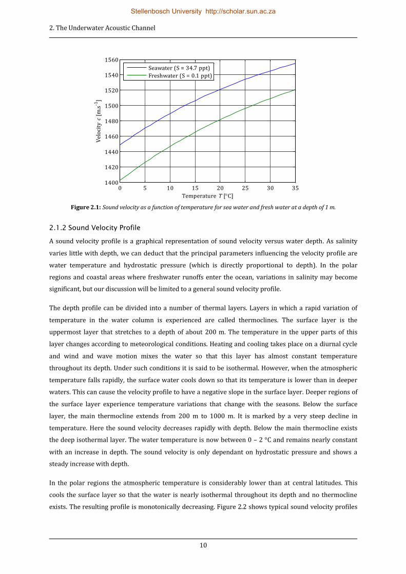
for agricultural usage is 2 ppt. Figure 2.1 shows the sound velocity as a function of temperature for
seawater and freshwater at a depth of 1 m.
Stellenbosch University http://scholar.sun.ac.za
2. The Underwater Acoustic Channel
10
Figure 2.1: Sound velocity as a function of temperature for sea water and fresh water at a depth of 1 m.
2.1.2 Sound Velocity Profile
A sound velocity profile is a graphical representation of sound velocity versus water depth. As salinity
varies little with depth, we can deduct that the principal parameters influencing the velocity profile are
water temperature and hydrostatic pressure (which is directly proportional to depth). In the polar
regions and coastal areas where freshwater runoffs enter the ocean, variations in salinity may become
significant, but our discussion will be limited to a general sound velocity profile.
The depth profile can be divided into a number of thermal layers. Layers in which a rapid variation of
temperature in the water column is experienced are called thermoclines. The surface layer is the
uppermost layer that stretches to a depth of about 200 m. The temperature in the upper parts of this
layer changes according to meteorological conditions. Heating and cooling takes place on a diurnal cycle
and wind and wave motion mixes the water so that this layer has almost constant temperature
throughout its depth. Under such conditions it is said to be isothermal. However, when the atmospheric
temperature falls rapidly, the surface water cools down so that its temperature is lower than in deeper
waters. This can cause the velocity profile to have a negative slope in the surface layer. Deeper regions of
the surface layer experience temperature variations that change with the seasons. Below the surface
layer, the main thermocline extends from 200 m to 1000 m. It is marked by a very steep decline in
temperature. Here the sound velocity decreases rapidly with depth. Below the main thermocline exists
the deep isothermal layer. The water temperature is now between 0 – 2 °C and remains nearly constant
with an increase in depth. The sound velocity is only dependant on hydrostatic pressure and shows a
steady increase with depth.
In the polar regions the atmospheric temperature is considerably lower than at central latitudes. This
cools the surface layer so that the water is nearly isothermal throughout its depth and no thermocline
exists. The resulting profile is monotonically decreasing. Figure 2.2 shows typical sound velocity profiles
0 5 10 15 20 25 30 351400
1420
1440
1460
1480
1500
1520
1540
1560
Temperature T [C]
Vel
oci
ty c
[m
.s-1
]
Seawater (S = 34.7 ppt)
Freshwater (S = 0.1 ppt)
Stellenbosch University http://scholar.sun.ac.za

2. The Underwater Acoustic Channel
11
of water at central latitudes and of polar waters. Note that these profiles can vary substantially with
latitude, season and oceanic and meteorological conditions.
Figure 2.2: Typical sound velocity profiles for central latitudes and polar regions.
2.2 Sound Propagation Paths
Urban [2] mentions that “when working with sound transmission in the ocean, it is desirable to know the
distribution of acoustic intensity with respect to depth, range and time.” Ray tracing is a method for
determining the paths of waves through a medium with varying propagation velocity, absorption
properties and reflective surfaces. In this section we will qualitatively apply ray tracing to the sound
velocity profile to predict the propagation of sound waves in the ocean.
2.2.1 Naturally Occurring Wave Guides
2.2.1.1 The Deep Sound Channel
From Figure 2.2 it is clear that at a certain depth between the main thermocline and the deep isothermal
layer, the sound velocity assumes a minimum value. This depth is defined as the axis of the deep sound
channel. The depth of the axis varies. It is deepest near the equator and moves to the surface at the poles.
On average it lies at about 1000 m.
Sound waves, as any other wave-like phenomenon, are subject to refraction when propagating through a
medium with varying properties. Refraction is a change in direction that a wave encounters, caused by a
change in its propagation velocity. The angle of refraction is always towards lower velocity.
Sound waves radiating from a source near the axis of the deep sound channel will refract in a direction
towards the axis where the velocity is a minimum. Given that the grazing angle between the direction of
propagation and the axis is sufficiently small, this will cause the sound waves to essentially oscillate about
the axis as it propagates. The sound waves are enclosed in a kind of natural waveguide called the deep
1440 1460 1480 1500 1520 1540 1560
0
500
1000
1500
2000
Velocity c [m.s-1]
De
pth
z [
m]
Surface layer
Main thermocline
Deep isothermal layer
Central latitudes
Polar regions
Stellenbosch University http://scholar.sun.ac.za

2. The Underwater Acoustic Channel
12
sound channel. The maximum grazing angle is a function of the gradient of the sound velocity profile and
the depth of the source. Urban determines the maximum grazing angle mathematically and also gives an
equation for the height of the channel [2]. Sound waves can propagate over great distances guided by the
deep sound channel, but it only exists in abyssal waters and is irrelevant for shallow water applications.
2.2.1.2 The Surface Channel
A similar waveguide like phenomenon occurs when the sound velocity profile exhibits a negative slope
towards the water surface. This is caused when the surface water has a lower temperature than deeper
waters or when the water is isothermal and the depth term in equation 2.1 results in a negative slope of
the sound velocity profile. Both the plots in Figure 2.2 show this characteristic.
Sound waves radiating from a source in the surface layer will be refracted toward the surface in the
direction of lower velocity. The water-air interface acts as a reflector and the sound waves are confined to
a natural occurring wave guide. As in the deep sound channel, a maximum grazing angle exists between
the propagation direction and the horizontal for which the sound waves will remain in the surface
channel. From Figure 2.2 it is intuitive that the height of the surface channel in polar regions will be much
greater than at the central latitudes where it is bounded by a local maximum in the sound velocity profile.
As the sound waves are reflected from the ocean surface, the state of the ocean will greatly influence its
propagation in the surface channel. A smooth surface will act as a near-perfect reflector while a rough
surface will scatter the reflections. Section 2.2.2 explains how surface roughness and wavelength
influence reflections.
2.2.1.3 The Shallow Water Waveguide
The refraction process described in the previous sections occurs over long distances in relatively deep
water. It applies to water bodies that are essentially semi-infinite, with the only boundary being the water
surface. For smaller, bounded water bodies we can simplify the propagation path prediction by assuming
isovelocity. Shallow water can be approximated as isothermal and the effect of the depth term of equation
2.1 is negligible, resulting in a constant sound velocity profile. Under these conditions we can make use of
straight-line ray traces to predict the propagation paths of sound waves.
Water bodies are bounded by an air-water interface at the surface and a water-floor interface at the
bottom. Depending on the properties of the bounding surface, an incident wave can be reflected, scattered
or partially transmitted. Air has negligible density so that the water-air interface introduces a perfect
reflection with 180° phase shift [4]. “For a simple ocean bottom which can be represented by a semi-
infinite half-space with constant sound speed and density... there exists a critical grazing angle below
which there is perfect bottom reflection” [4]. We can apply Snell’s Law, given in equation 2.2, to
determine this angle.
(2.2)
Stellenbosch University http://scholar.sun.ac.za

2. The Underwater Acoustic Channel
13
By taking the sound velocity in water as c1 = 1500 m.s-1 and in the ocean floor as c2 = 5000 m.s-1, θc
equates to 72.54 °. Therefore waves emitted within a 2θc cone will propagate unattenuated down a
perfectly smooth, semi-infinite waveguide bounded only by the surface and bottom. Figure 2.3 shows ray-
traces of waves propagating along the shallow water waveguide.
Figure 2.3: Wave propagation along the shallow water waveguide.
2.2.2 Scattering
Up to now we have considered propagation paths under the assumption that all bounding surfaces are
perfectly smooth and all reflections are lossless. Apart from temperature and the depth-pressure relation
that influence the sound velocity profile, we have also regarded water as a homogeneous medium. While
these conditions can be approximated in a controlled environment, we can expect deviating results when
applying these theories to actual field scenarios.
The ocean surface and floor are rarely flawlessly smooth. While smooth surfaces act as perfect reflectors,
rough surfaces can severely scatter incident waves. Ogilvy uses the root mean square (RMS) deviation
from the smooth plane and the power spectrum density of a randomly varying surface to describe its
roughness [5]. He explores several different models for determining scattering behaviour of waves. For
our purposes it is sufficient to note that the roughness of a surface should be regarded relative to the
wavelength of an incident wave. Waves reflected off surfaces with roughness parameters of the same
order of magnitude as its wavelength, will undergo scattering. Waves with a wavelength that is orders of
magnitude larger than a surface’s roughness will be nearly coherently reflected. For example, an ocean
floor lined with pebbles with an average diameter of 50 mm will reflect a low frequency wave with a
wavelength of 30 m with minimal loss of coherence, while it will severely scatter a high frequency wave
with a wavelength of 100 mm. The same applies to the water surface. Choppy water will scatter short
wavelengths, but will not affect the reflection of long wavelengths. It is clear that rough ocean conditions
2θc
Stellenbosch University http://scholar.sun.ac.za

2. The Underwater Acoustic Channel
14
and an irregular ocean bottom will mar wave propagation along the surface channel and shallow water
waveguide.
Shoals of fish and other marine life forms, suspended air bubbles created by wave action, and other
inhomogeneous objects in shallow water also contribute to scattering of sound waves. Many works
further investigate this subject and give mathematical models to predict scattering effects. It is sufficient
to note that small inhomogeneities (relative to the wavelength) can cause a loss of coherence as incident
waves tend to diffract around it. Large objects will obstruct sound waves causing shadow zones to occur.
2.3 The Underwater Environment as a Communication Channel
In the previous sections we qualitatively explore general characteristics of sound propagation in water. It
is clear that the underwater environment can present greatly varying conditions. Factors such as the
reflection, refraction and scattering of sound waves are highly dependent on the particular circumstances.
To accurately predict the characteristics of the underwater channel we would have to take into account
the specific setting and environmental conditions. For this project however, we endeavour to provide an
adaptable modem that will perform well under a range of conditions. To realise this, we consider practical
worst case scenarios and tailor our design to deal with such conditions.
In this section we investigate aspects of the underwater environment that specifically pertain to the
communication channel. These include multipath propagation, transmission losses, frequency dependant
attenuation, the Doppler Effect and additive noise.
2.3.1 Multipath Propagation
In wireless communications, fading refers to a time-varying, frequency dependent, loss of received signal
strength. Fading can be multipath induced or due to shadowing from objects obstructing the signal path.
Multipath propagation occurs when numerous versions of a transmitted signal reach the receiver along
different propagation paths. The received duplicates of the original signal can encounter different time-
delays, attenuation, phase shifts and frequency shifts. These signals superimpose to form a resultant
signal of greater or lower amplitude, a phenomenon called interference. As a consequence of the
coalescing signals, the received signal is often highly distorted.
In the underwater environment, surface and bottom reflections contribute to severe multipath distortion.
To predict the effects of multipath propagation we construct a simplified model of a typical worst case
underwater channel. Let us consider a semi-infinite water body with isovelocity. Straight-line ray traces
can be used to identify propagations paths between the transmitter and receiver. These paths are called
eigenpaths. By calculating the distance of each eigenpath and dividing it by the sound velocity, we can
determine the time spreading of reflections arriving at the receiver. If we take into account that no
bounding surface is completely smooth and lossless, an incident wave will suffer partial scattering and
absorption by the receiving medium. Figure 2.4 shows the direct eigenpath and a number of reflected
eigenpaths as well as scattering losses.
Stellenbosch University http://scholar.sun.ac.za

2. The Underwater Acoustic Channel
15
Figure 2.4: Ray traces of multipath propagation in a practical scenario.
Indices are used to indicate the number of reflections from the surface and bottom. Every surface
reflection will introduce a 180 ° phase shift and scattering. A lossy bottom will partially absorb incident
wave energy and also scatter the reflected wave. The more times a wave is reflected, the more it will be
attenuated due to absorption and scattering, until it eventually becomes negligibly small.
From this qualitative description, we expect the channel impulse response to consist of a larger preceding
impulse followed by many smaller impulses with ever increasing attenuation. The larger impulse
corresponds to the direct path and the smaller ones represent the arrival of the different reflected waves
at the receiver.
2.3.2 Doppler Effect
The Doppler Effect describes the shift in observed frequency of acoustic waves when a transmitter and
receiver are in motion relative to each other and/or the medium. The observed frequency will be higher
as the transmitter and receiver approach each other and lower as they depart. Depending on the
movement of the transmitter and receiver the Doppler Effect can vary in its occurrence. A stationary
transmitter will emit acoustic waves with uniform wavelength in all directions, while a moving
transmitter will create a wave field with wavelengths dependent on direction. We recognise two cases of
the Doppler effect: one-way propagation where the received signal is from a remote transmitter and two-
way propagation where the received signal is echoed from an object. The frequency shift from two-way
propagation is often used in sonar applications to determine the velocity of an object. One-way
propagation is primarily applicable to communication channels, although two-way propagation can occur
when the signal is reflected from a moving object.
For a transmitter and receiver that have constant velocity in a stationary medium the observed frequency
can be determined as:
(0,0)
(0,1)
(1,1) Transmitter
Receiver
2θc
(1,0)
Stellenbosch University http://scholar.sun.ac.za

2. The Underwater Acoustic Channel
16
(2.3)
and denote the observed and transmitted frequencies respectively. is the velocity of sound in
water. and are the components of the transmitter and receiver velocity in the direction of the
direct path between them.
If the velocity of the transmitter and receiver is small in comparison with the sound velocity, so that
, equation 2.3 can be approximated as
(
) (2.4)
The ratio of
is known as the Doppler ratio.
In comparison with other wireless channels, the Doppler Effect can be fairly pronounced in the
underwater environment. Consider an underwater ROV capable of speeds up to 10 km/h or 2.778 m/s. If
it receives control signals from a stationary transmitter while travelling rectilinearly towards it at full
speed, the Doppler ratio can be determined as:
(
)
(
)
(2.5)
If the modulated signal has a carrier frequency of 50 kHz, this results in a observed frequency of:
( )
( )
(2.6)
2.3.3 Coherence Bandwidth and Coherence Time
The two key distortion effects that will have the most pronounced influences on the signal as it traverses
the underwater channel is multipath propagation and Doppler frequency shifts. In the previous two
subsections we have investigated the mechanics of these phenomena, but now we are interested in the
anticipated influences it will have on the time and frequency behaviour of the channel.
The delay spread of a channel is a parameter that describes its time dispersive nature. It is essentially a
measure of the duration of the impulse response of a channel. Alternatively, it can be viewed as the time
delay between the first arrival of a transmitted signal and the last multipath reflection at the receiver. The
frequency domain equivalent of the delay spread is the coherence bandwidth.
The coherence bandwidth of a channel is a measure of the frequency interval over which the channel’s
frequency response can be considered as flat, i.e. the maximum bandwidth over which frequency
components experience equal or comparable fading. The coherence bandwidth can be approximated as
Stellenbosch University http://scholar.sun.ac.za

2. The Underwater Acoustic Channel
17
(2.7)
where denotes the channel delay spread.
Let’s consider a scenario where the last reflected version of a transmitted signal to reach the receiver
travels 100 m more than the first directly received signal. Travelling at 1500 m/s, the signal will
experience a delay spread of 66.7 ms. The resultant coherence bandwidth of the channel is ⁄
.
Ideally we would define the symbol duration of the transmitted signal to last longer than the delay spread
of the channel in order to mitigate intersymbol inference. However, if we make the symbol duration too
long, we run the risk that the channel characteristics might change during the transmission of the symbol.
This is especially true for mobile applications where the coherence time of the channel can be fairly short.
Doppler spread is a measure of the spectral broadening caused by the time rate of change of the mobile
channel [7]. A purely sinusoidal signal suffering from a Doppler frequency shift of will experience so-
called spectral broadening so that it has components in the range of to .
The coherence time is the time domain equivalent of the Doppler spread and is used to characterise the
time varying nature of the frequency dispersiveness of the channel in the time domain [7]. Alternatively,
the coherence time can be viewed as a statistical measure of the time duration over which the channel
impulse response is essentially invariant [7]. The maximum Doppler shift and time coherence is
inversely proportional so that
(2.8)
A conservative rule of thumb for modern digital communication [7] is to define the coherence time as
(2.9)
The definition of time coherence implies that two signals arriving with a time separation of greater than
are affected differently the channel [7].
Returning to the ROV scenario in Section 2.3.2 we have that the maximum Doppler shift is .
This equates to a conservative time coherence of . Thus, as long the symbol duration of the
signal is shorter than 4.6 ms it should not suffer from distortion due to frequency dispersion.
However, we have just shown that in order to avoid intersymbol interference due to the delay spread, the
symbol duration should be longer than 66.7 ms. This contradiction is what defines the challenge of
underwater communication. A suitable modulation technique would have to provide some method of
compensating for the Doppler spread of the channel while still maintaining a slow symbol rate.
Stellenbosch University http://scholar.sun.ac.za

2. The Underwater Acoustic Channel
18
2.3.4 Propagation Loss
Propagation loss defines the decrease of acoustic intensity of a sound wave as it propagates from a
transmitter to a receiver. Urban divides propagation losses into three parts: losses caused by geometrical
spreading, attenuation due to frequency dependent absorption and a so-called anomaly that accounts for
all other losses [2]. These include leakage of waveguides, scattering and diffraction. In this section we
discuss geometric spreading and absorption.
We define acoustic intensity of a source as at a range of . At a distance r from the source the
intensity is . The ratio between these two intensities determines the propagation loss. As noted the
intensity is range and frequency dependent.
2.3.4.1 Geometric Spreading
Geometric spreading is the exponential decrease in intensity with range. Acoustic intensity is defined as
the radiated power per unit area . At the reference distance and at an arbitrary distance
from the source the intensities and are
(2.10)
and
(2.11)
The spreading loss is
(2.12)
We have that the spreading loss is only dependent on the irradiated area. If the shape of the area is know,
equation 2.12 can be further reduced to a function of range only.
Two types of spreading occur that will determine the shape of irradiance. Spherical spreading takes place
in infinite water bodies where the power emitted by a source radiates uniformly in all directions. The
area of a sphere is
(2.13)
The spreading loss for spherical spreading is thus
Stellenbosch University http://scholar.sun.ac.za

2. The Underwater Acoustic Channel
19
(
)
(2.14)
The intensity of the emitted signal decreases with .
Cylindrical spreading exists in semi-infinite water bodies bounded by a perfectly reflective surface and
bottom. For a water depth of ten times or more than the wavelength of the emitted signal and for a range
much greater than the depth, the spreading can be approximated as cylindrical. The irradiated surface
has an area of
(2.15)
The spreading loss for cylindrical spreading is
(2.16)
The intensity of the emitted signal decreases linearly with .
We note that spherical and cylindrical spreading differs in the exponent of range. By taking as the
exponent, we can determine the transmission loss, the logarithmic expression of spreading loss in decibel,
as
(
)
(
)
(
)
(2.17)
where for cylindrical spreading and for spherical spreading. In some cases where the range
is in the transition zone between spherical and cylindrical, is taken as a fractional number, .
2.3.4.2 Attenuation by Absorption
Absorption is the process whereby the acoustic energy of a wave is converted into heat. This is induced
by internal friction, internal heat dissipation and the effects of relaxation. The attenuation of the pressure
amplitude of an acoustic wave shows exponential decay with range, so that we may write
( ) (2.18)
Stellenbosch University http://scholar.sun.ac.za
2. The Underwater Acoustic Channel
20
where and denote the pressure amplitude of the acoustic wave at unit distance and at an
arbitrary distance . is the amplitude attenuation coefficient in Nepers per meter. Acoustic intensity is
proportional to the square of the amplitude, so that the acoustic intensity decreases by a factor ( ).
Absorption is frequency dependent, so that higher frequencies suffer greater attenuation. We adapt the
attenuation factor to include the frequency dependence, so that the absorption loss becomes
(
)
( ) ( ) (2.19)
The transmission loss in logarithmic notation is
(
)
( ( ) ( ))
( ) ( )
( ) ( ) (2.20)
The attenuation coefficient ( ) has the unit of Np.m-1 and its decibel equivalent is ( ) in dB/m. The
conversion factor between ( ) in and ( ) is:
( ) ( )
( ) (2.21)
In liquids the effects of internal friction and internal heat dissipation are responsible for the absorption of
acoustic energy. Urban [2] gives the attenuation coefficient for liquids as
(
( )
)
(2.22)
attenuation coefficient, Np/m
frequency, Hz
density, kg/m3
sound velocity, m/s
shear component of viscosity, Ns.m2
heat conductivity, W/(m.°K)
ratio of specific heats
specific heat at constant pressure, J/(kg. °K)
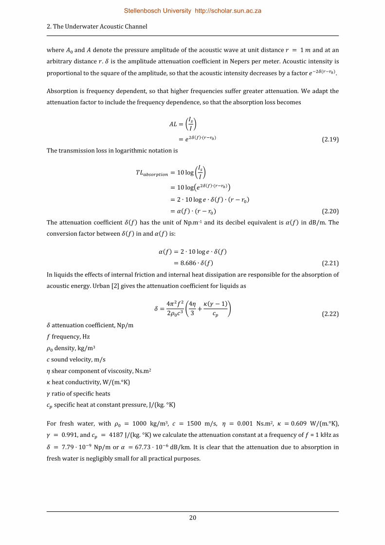
For fresh water, with kg/m3, m/s, Ns.m2, W/(m.°K),
, and J/(kg. °K) we calculate the attenuation constant at a frequency of = 1 kHz as
Np/m or dB/km. It is clear that the attenuation due to absorption in
fresh water is negligibly small for all practical purposes.
Stellenbosch University http://scholar.sun.ac.za
2. The Underwater Acoustic Channel
21
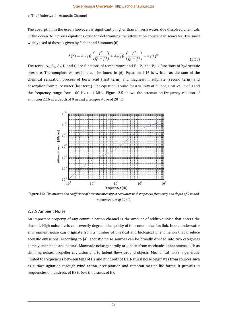
The absorption in the ocean however, is significantly higher than in fresh water, due dissolved chemicals
in the ocean. Numerous equations exist for determining the attenuation constant in seawater. The most
widely used of these is given by Fisher and Simmons [6]:
( ) (
) (
)
(2.23)
The terms A1, A2, A3, f1 and f2 are functions of temperature and P1, P2 and P3 is functions of hydrostatic
pressure. The complete expressions can be found in [6]. Equation 2.16 is written as the sum of the
chemical relaxation process of boric acid (first term) and magnesium sulphate (second term) and
absorption from pure water (last term). The equation is valid for a salinity of 35 ppt, a pH-value of 8 and
the frequency range from 100 Hz to 1 MHz. Figure 2.5 shows the attenuation-frequency relation of
equation 2.16 at a depth of 0 m and a temperature of 20 °C.
Figure 2.5: The attenuation coefficient of acoustic intensity in seawater with respect to frequency at a depth of 0 m and
a temperature of 20 °C.
2.3.5 Ambient Noise
An important property of any communication channel is the amount of additive noise that enters the
channel. High noise levels can severely degrade the quality of the communication link. In the underwater
environment noise can originate from a number of physical and biological phenomenon that produce
acoustic emissions. According to [4], acoustic noise sources can be broadly divided into two categories
namely, manmade and natural. Manmade noise generally originates from mechanical phenomena such as
shipping noises, propeller cavitation and turbulent flows around objects. Mechanical noise is generally
limited to frequencies between tens of Hz and hundreds of Hz. Natural noise originates from sources such
as surface agitation through wind action, precipitation and cetacean marine life forms. It prevails in
frequencies of hundreds of Hz to low thousands of Hz.
102
103
104
105
106
10-3
10-2
10-1
100
101
102
103
Frequency f [Hz]
Att
en
ua
tio
n
[d
B/
km]
Stellenbosch University http://scholar.sun.ac.za

2. The Underwater Acoustic Channel
22
The noise levels in the underwater environment vary greatly between different locations. Any attempt at
predicting a generally applicable noise level is futile. We accept that some level of ambient noise will
always be present and that if accurate values are needed for a design it is best to practically measure it.
2.4 Summary
From the above it is clear that the marine environment is a very challenging one from a communications
point of view. Multipath propagation and noise levels are generally severe and significantly variable. Any
successful design should therefore include some form of compensation to increase robustness. This is
further discussed in the next chapter.
Stellenbosch University http://scholar.sun.ac.za
23
3 OFDM: THE MODULATION SCHEME OF CHOICE
To transfer a message from a source to a destination via a wireless communication link, we generally use
a carrier signal, modulated according to the specification of a modulation scheme, to “carry” the message.
In the case of digital modulation, the message will consist of a series of symbols, each representing a
binary data sequence. Depending on the modulation scheme, the amplitude, phase or frequency of the
carrier signal can be controlled to represent the different message symbols. The choice of modulation
scheme will mainly depend on the properties of the particular communication channel. Secondary factors,
such as the available bandwidth, throughput requirements, limitations of hardware and implementation
cost, come into play thereafter.
In the previous chapter we investigated the underwater environment as a communication channel and
we identify the main distorting phenomena that a signal can experience. With this in mind we now
endeavour to find a modulation scheme with the capabilities to perform efficiently under the conditions
set by the underwater environment.
3.1 Orthogonal Multicarrier Modulation
3.1.1 Concept of Multicarrier Modulation
Intersymbol interference (ISI) is caused by multipath propagation when the reflections of previously
transmitted symbols are delayed to such an extent that they arrive at the receiver together with a
subsequent symbol. The time delay between the arrival of the first version of a transmitted symbol and
the last reflected version is called the channel delay spread. For reception free of ISI, the symbol duration
has to be much longer than the channel delay spread , so that
(3.1)
In Section 2.3.3, we calculated the delay spread of a typical underwater environment as in the order of
66.7 ms. For illustrative purposes, let us consider the data rate requirement of 20kbps, set in Chapter 1.
Assuming single carrier modulation with a symbol rate of and 1 bit per symbol, the symbol duration is
(3.2)
When comparing these numbers it is clear that a single carrier modulation scheme will suffer severe ISI in
the underwater environment.
In order to prolong the symbol duration while maintaining the data rate we resort to multicarrier
modulation. By this concept the original serial symbol stream is divided into parallel streams, each with
Stellenbosch University http://scholar.sun.ac.za
3. OFDM: The Modulation Scheme of Choice
24
a lower symbol rate of ⁄ . A series of adjacent subcarriers at different frequencies are simultaneously
modulated by the parallel symbol streams. This can be regarded as parallel transmission in the frequency
domain. The total bandwidth occupied by the signal remains unaffected, because by effectively increasing
the symbol duration by a factor , the bandwidth occupied by each of the subcarriers is reduced to ⁄
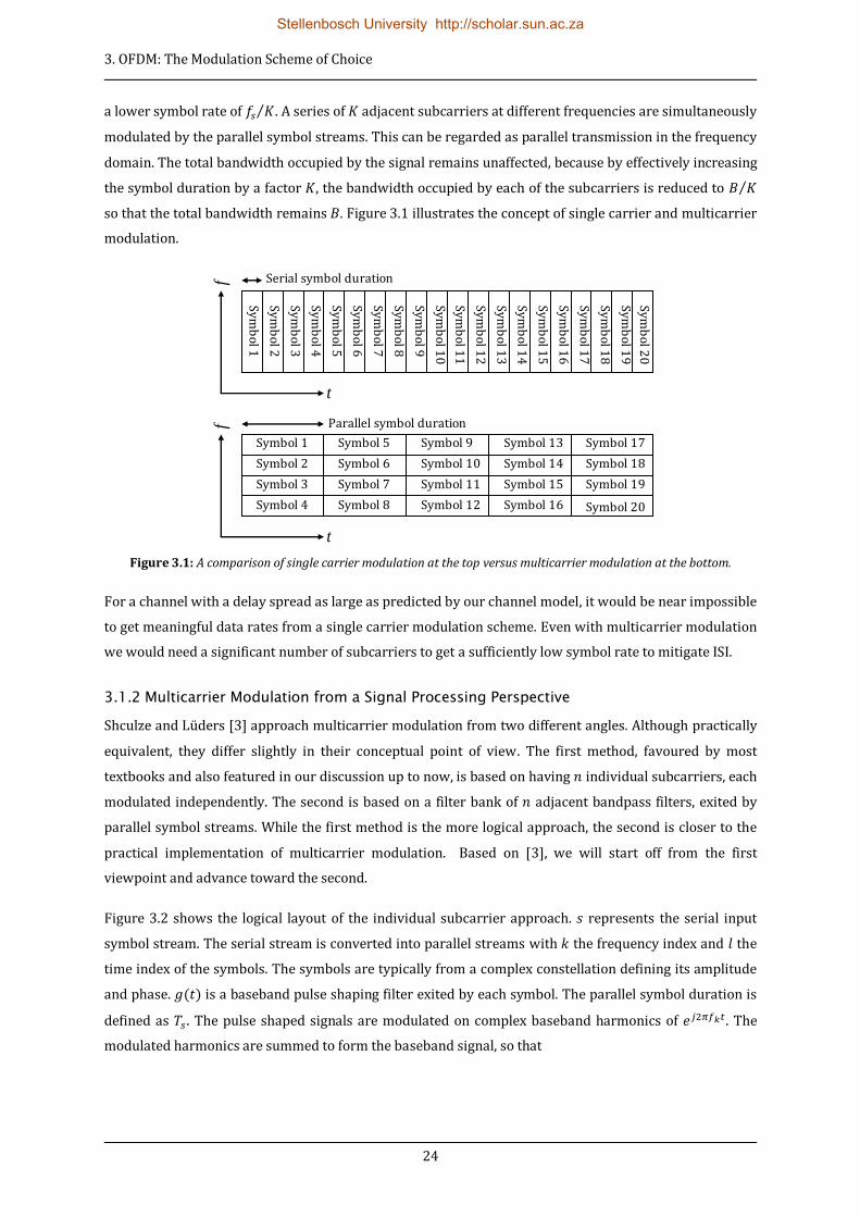
so that the total bandwidth remains . Figure 3.1 illustrates the concept of single carrier and multicarrier
modulation.
Figure 3.1: A comparison of single carrier modulation at the top versus multicarrier modulation at the bottom.
For a channel with a delay spread as large as predicted by our channel model, it would be near impossible
to get meaningful data rates from a single carrier modulation scheme. Even with multicarrier modulation
we would need a significant number of subcarriers to get a sufficiently low symbol rate to mitigate ISI.
3.1.2 Multicarrier Modulation from a Signal Processing Perspective
Shculze and Lüders [3] approach multicarrier modulation from two different angles. Although practically
equivalent, they differ slightly in their conceptual point of view. The first method, favoured by most
textbooks and also featured in our discussion up to now, is based on having individual subcarriers, each
modulated independently. The second is based on a filter bank of adjacent bandpass filters, exited by
parallel symbol streams. While the first method is the more logical approach, the second is closer to the
practical implementation of multicarrier modulation. Based on [3], we will start off from the first
viewpoint and advance toward the second.
Figure 3.2 shows the logical layout of the individual subcarrier approach. represents the serial input
symbol stream. The serial stream is converted into parallel streams with the frequency index and the
time index of the symbols. The symbols are typically from a complex constellation defining its amplitude
and phase. ( ) is a baseband pulse shaping filter exited by each symbol. The parallel symbol duration is
defined as . The pulse shaped signals are modulated on complex baseband harmonics of . The
modulated harmonics are summed to form the baseband signal, so that
Sym
bol 1
Sym
bol 2
Sym
bol 3
Sym
bol 4
Sym
bol 5
Sym
bol 6
Sym
bol 7
Sym
bol 8
Sym
bol 9
Sym
bol 1
0
Sym
bol 1
1
Sym
bol 1
2
Sym
bol 1
3
Sym
bol 1
4
Sym
bol 1
5
Sym
bol 1
6
Sym
bol 1
7
Sym
bol 1
8
Sym
bol 1
9
Sym
bol 2
0
Symbol 1
Symbol 2
Symbol 3
Symbol 4
Symbol 5
Symbol 6
Symbol 7
Symbol 8
Symbol 9
Symbol 10
Symbol 11
Symbol 12
Symbol 13
Symbol 14
Symbol 15
Symbol 16
Symbol 17
Symbol 18
Symbol 19
Symbol 20
Parallel symbol duration
Serial symbol duration ff
t
t
Stellenbosch University http://scholar.sun.ac.za

3. OFDM: The Modulation Scheme of Choice
25
( ) ∑
∑ ( )
(3.3)
Figure 3.2: Block diagram of subcarrier based multicarrier transmission.
To lead us to the second filter bank modulation method, we consider that the pulse shaping filters and the
complex harmonic modulation can be combined. Up to now we assumed ( ) to be identical pulse
shaping filters. By “pre-shifting” every pulse shape with its corresponding modulating frequency, we end
up with a bank of parallel band pass filters. Figure 3.3 shows the concept of filter bank modulation. For
obtaining frequency shifted versions of the pulse shape we can write
( ) ( ) (3.4)
For each time instant , a set of parallel symbols excites the frequency shifted pulse shaping filters. The
outputs of the filter bank are summed to form the complex baseband signal
( ) ∑∑ ( )
(3.5)
By defining ( ) as
( ) ( ) (3.6)
we can rewrite equation 3.5 in its compact form as
( ) ∑ ( )
(3.7)
Figure 3.3: Block diagram of filter bank based multicarrier transmission.
S/P
g(t)
g(t)
Σ s(t) s
2π kj f te
12
π kj f te
12
π kj f te
g(t)
pk-1,l
pk,l
pk+1,l
· · ·
· · ·
S/P
gk-1(t)
gk+1(t)
Σ s(t) s gk(t)
pk-1,l
pk,l
pk+1,l
· · ·
· · ·
Stellenbosch University http://scholar.sun.ac.za

3. OFDM: The Modulation Scheme of Choice
26
To draw a mathematical comparison between the subcarrier and filter bank approaches, we fully expand
equation 3.5 to
( ) ∑ ( ) ( )
(3.8)
Note that if we substitute in equation 3.3 with we get
( ) ∑
∑ ( )
∑ ( ) ( )
(3.9)
This is the same as equation 3.8 for the filter bank method. The time-frequency-dependant phase shift
introduced into each symbol by does not influence the workings of the modulation process, so
that the two methods can be regarded as mathematically equivalent.
Up to now we have made no reference to the shape of the pulse shaping filter ( ). Consider a simple
rectangular pulse of duration , so that
( ) (
) (3.10)
A rectangular time pulse has a Fourier transform of an infinitely spread function in the frequency domain
so that,
( ) (
) (3.11)
This relation is shown in Figure 3.4.
Figure 3.4: Fourier transform pair of rectangular pulse.
We defined ( ) as the frequency shifted equivalent of ( ), so that
( ) (
) (3.12)
Equation 3.12 can be interpreted as the modulation of a complex periodic time signal by a rectangular
pulse, as illustrated by Figure 3.5. (Due to the difficulty of plotting a complex wave, ( ) is represented
here only by its real part, although the spectrum is single sided.) By the properties of the Fourier
transform, a frequency shift of will result in
t
g(t)
2s
T
2s
T
1
0 f
G(f)
1
sT
2
sT
1
sT
2
sT
0
Stellenbosch University http://scholar.sun.ac.za
3. OFDM: The Modulation Scheme of Choice
27
( ) (
( )
)
(3.13)
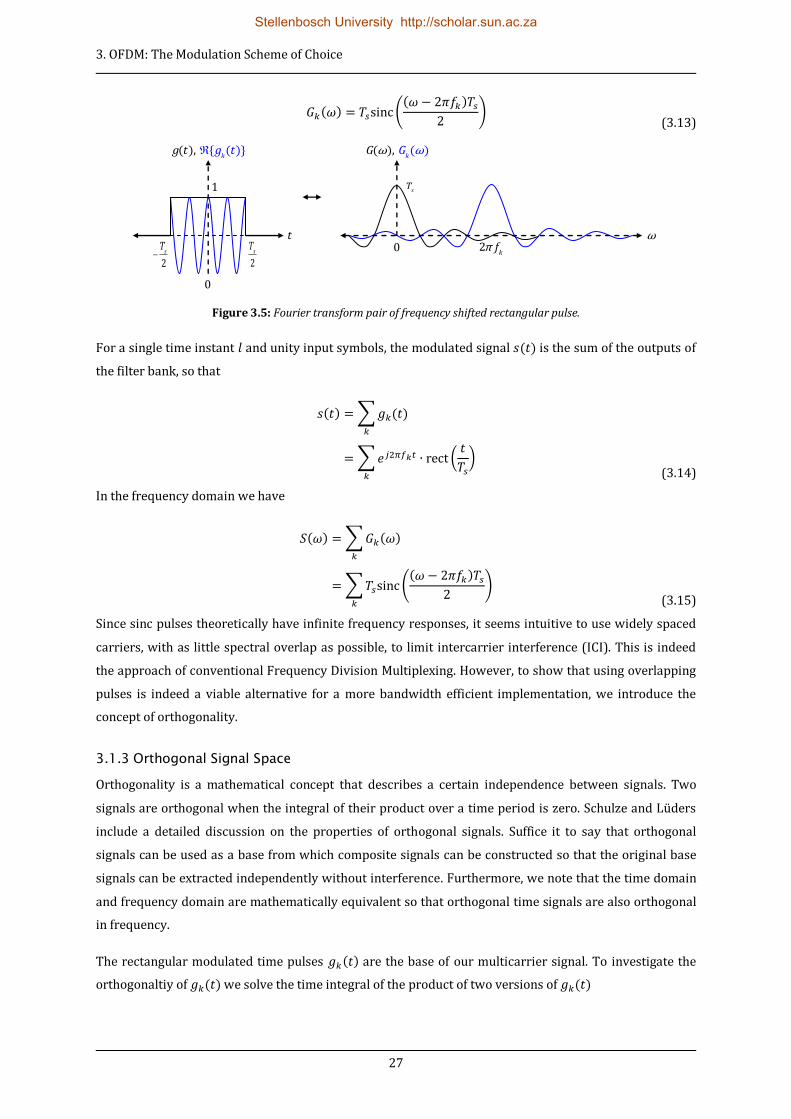
Figure 3.5: Fourier transform pair of frequency shifted rectangular pulse.
For a single time instant and unity input symbols, the modulated signal ( ) is the sum of the outputs of
the filter bank, so that
( ) ∑ ( )
∑ (
)
(3.14)
In the frequency domain we have
( ) ∑ ( )
∑ (( )
)
(3.15)
Since sinc pulses theoretically have infinite frequency responses, it seems intuitive to use widely spaced
carriers, with as little spectral overlap as possible, to limit intercarrier interference (ICI). This is indeed
the approach of conventional Frequency Division Multiplexing. However, to show that using overlapping
pulses is indeed a viable alternative for a more bandwidth efficient implementation, we introduce the
concept of orthogonality.
3.1.3 Orthogonal Signal Space
Orthogonality is a mathematical concept that describes a certain independence between signals. Two
signals are orthogonal when the integral of their product over a time period is zero. Schulze and Lüders
include a detailed discussion on the properties of orthogonal signals. Suffice it to say that orthogonal
signals can be used as a base from which composite signals can be constructed so that the original base
signals can be extracted independently without interference. Furthermore, we note that the time domain
and frequency domain are mathematically equivalent so that orthogonal time signals are also orthogonal
in frequency.
The rectangular modulated time pulses ( ) are the base of our multicarrier signal. To investigate the
orthogonaltiy of ( ) we solve the time integral of the product of two versions of ( )
t
2s
T
2s
T
0
ω 2
kfπ0
sT1
kG G), )( (ω ω
kg tt g), (( )
Stellenbosch University http://scholar.sun.ac.za

3. OFDM: The Modulation Scheme of Choice
28
∫ ( ) ( )
∫ (
)
(
)
∫ ( )
( ) ( ) |
( )
( )
( )
( ( ) )
( )
(3.16)
For ( ) and ( ) to be orthogonal, equation 3.16 must be equal to zero. This holds for integer values
of ( ) . By defining the frequency shifts as multiples of the symbol rate, so that ⁄ and
⁄ , we achieve orthogonality between ( ) and ( ). We expand this to include all of ( )
by defining as harmonics of the symbol rate for subcarriers
(3.17)
Figure 3.6 shows the frequency shifted sinc pulses ( ), aligned with the zero crossings of the baseband
sinc, ( ), at harmonics of
. For reasons due to practical implementation, , corresponding to the dc
component of the signal, is generally left unoccupied.
Figure 3.6: Frequency response of multiple sinc pulses.
To return to the question at the end of the previous section, we can now conclude that the rectangular
pulses ( ), modulated at harmonics of the parallel symbol rate, do indeed form an orthogonal base
from which the multicarrier signal can be constructed. Their orthogonality ensures that a demodulator
can successfully extract the individual carriers without ICI, even though their frequency responses
overlap.
3.2 Orthogonal Frequency Division Multiplexing
The parallel transmission of multiple symbols on orthogonal carriers is known as Orthogonal Frequency
Division Multiplexing (OFDM). OFDM was originally proposed by Chang [8] in 1960 but it largely
sT
. . . 2
s
π
T
2
s
π
Ts
Kπ
T
s
Kπ
T
4
s
π
T
4
s
π
T. . .
ω
0
k
G ωωG ), (( )
Stellenbosch University http://scholar.sun.ac.za
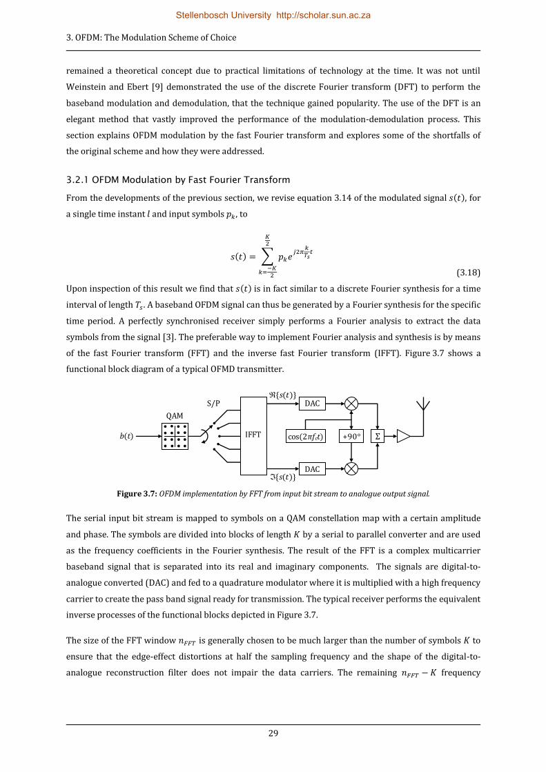
3. OFDM: The Modulation Scheme of Choice
29
remained a theoretical concept due to practical limitations of technology at the time. It was not until
Weinstein and Ebert [9] demonstrated the use of the discrete Fourier transform (DFT) to perform the
baseband modulation and demodulation, that the technique gained popularity. The use of the DFT is an
elegant method that vastly improved the performance of the modulation-demodulation process. This
section explains OFDM modulation by the fast Fourier transform and explores some of the shortfalls of
the original scheme and how they were addressed.
3.2.1 OFDM Modulation by Fast Fourier Transform
From the developments of the previous section, we revise equation 3.14 of the modulated signal ( ), for
a single time instant and input symbols , to
( ) ∑
(3.18)
Upon inspection of this result we find that ( ) is in fact similar to a discrete Fourier synthesis for a time
interval of length . A baseband OFDM signal can thus be generated by a Fourier synthesis for the specific
time period. A perfectly synchronised receiver simply performs a Fourier analysis to extract the data
symbols from the signal [3]. The preferable way to implement Fourier analysis and synthesis is by means
of the fast Fourier transform (FFT) and the inverse fast Fourier transform (IFFT). Figure 3.7 shows a
functional block diagram of a typical OFMD transmitter.
Figure 3.7: OFDM implementation by FFT from input bit stream to analogue output signal.
The serial input bit stream is mapped to symbols on a QAM constellation map with a certain amplitude
and phase. The symbols are divided into blocks of length by a serial to parallel converter and are used
as the frequency coefficients in the Fourier synthesis. The result of the FFT is a complex multicarrier
baseband signal that is separated into its real and imaginary components. The signals are digital-to-
analogue converted (DAC) and fed to a quadrature modulator where it is multiplied with a high frequency
carrier to create the pass band signal ready for transmission. The typical receiver performs the equivalent
inverse processes of the functional blocks depicted in Figure 3.7.
The size of the FFT window is generally chosen to be much larger than the number of symbols to
ensure that the edge-effect distortions at half the sampling frequency and the shape of the digital-to-
analogue reconstruction filter does not impair the data carriers. The remaining frequency
IFFT
DAC
DAC
Σ
S/P
QAM
+90° cos(2πfct) b(t)
( ) s t
( ) s t
Stellenbosch University http://scholar.sun.ac.za

3. OFDM: The Modulation Scheme of Choice
30
coefficients are left unoccupied. Figure 3.8 compares the nominal channel bandwidth and bandwidth
occupied by the data carriers.
Figure 3.8: Frequency occupation by data carriers.
3.2.2 Guard Intervals
From our discussion on multipath propagation we know that delayed reflections of the original
transmitted signal will add to distortion of the received signal. We succeeded in significantly prolonging
our symbol duration with multicarrier modulation, but there remains a period at the beginning of each
subsequent symbol for which the reflections of the previous symbol will interfere with it. A simple
solution is to insert a guard interval between symbols so that interfering reflections of a previous symbol
have time to die down. The periodic nature of Fourier synthesis lends itself to cyclic extension so that a
section from the end of an OFDM symbol can be prefixed to it without the loss of orthogonality of the
carriers. The cyclic prefix “absorbs” the multipath interference of the previous symbol so that the
subsequent symbol remains unaffected. Figure 3.9 illustrates the benefit of cyclic prefixing. The duration
of the guard interval will depend on the channel delay spread and varies between
and
for practical
systems. The trade off between less interference and lower data rates should be considered when
determining the length of the guard interval.
Figure 3.9: OFMD signals with and without cyclic prefix.
2s
f
2
s
f
Nominal channel bandwidth
Occupied bandwidth
f
Amplitude
s
FFT
ff
n
OFDM symbol l OFDM symbol l+1
OFDM symbol l OFDM symbol l+1 Guard interval
Overlap with delayed reflection
Cyclic prefix
Stellenbosch University http://scholar.sun.ac.za

3. OFDM: The Modulation Scheme of Choice
31
3.2.3 Time Synchronisation
Up to now we have considered only perfectly synchronised systems that can extract sequential OFDM
symbols with perfect timing. Considering the low symbol rate and the further addition of a cyclic prefix,
an OFDM signal is in fact reasonably robust against timing errors. Assuming little multipath delay spread
and a long cyclic prefix of , a tolerance in positioning of the FFT window of up to a 20% of the total
symbol length can be realised. The resulting phase shift of the subcarriers from a misaligned FFT window
can easily be corrected by channel estimation techniques.
Various methods of timing synchronisation exist. The simplest is probably the insertion of a null symbol
at the beginning of each frame to be detected by an envelope detector. While not very accurate, this
method can at least provide coarse timing alignment. An alternative is the insertion of a known reference
symbol at the beginning of each frame. A well designed reference symbol will not only provide accurate
timing alignment, but also serve in the channel estimation process. The subcarriers of the reference
symbol are modulated by a set of known complex symbols. The symbols should have equal amplitude and
random phase to provide a white noise-like frequency response and an impulse-like autocorrelation
function. By cross correlating the received signal with the reference symbol, peaks can be observed at
instances of the received symbol. For symbols with impulse-like autocorrelation properties, the channel
impulse response can be determined from the cross correlation. Positioning of the FFT window is done by
aligning it with the strongest peak in the cross correlation. The received reference symbol can also aid in
channel estimation by evaluating the change in amplitude and phase of each of the subcarriers from its
original state.
Another method makes use of the repeating portions of cyclically extended symbols to determine the
symbol timing. By using sliding window autocorrelation of the received signal and extracting the peaks of
the cyclic extensions, we can determine the positions of the symbols and so the alignment of the FFT
window.
3.2.4 Frequency Synchronisation
Although the timing requirements of an OFDM signal is fairly relaxed, the close spacing of adjacent
subcarriers requires highly accurate frequency synchronisation between the transmitter and receiver.
Dependent on the severity of a frequency mismatch, different effects are observed. Larger frequency
offsets corrupt the orthogonality between subcarriers and causes significant ICI. Smaller frequency
mismatches causes a frequency dependent phase rotation of the received symbols. Figure 3.11 shows
how he extracted QAM symbols are essentially smeared in a circular fashion about the origin of the
constellation diagram. This rotation is easily corrected by means of channel estimation.
A frequency mismatch can be interpreted as a translation of the received signal in the frequency domain.
The nodes of the sinc pulses will no longer align with the frequency coefficients of the Fourier analysis, so
that adjacent carriers cannot be extracted without interference from one another. Figure 3.10 illustrates
how a frequency offset corrupts orthogonality and causes ICI.
Stellenbosch University http://scholar.sun.ac.za

3. OFDM: The Modulation Scheme of Choice
32
Figure 3.10: The misalignment of the Fourier coefficients with the received sinc pulses due to a frequency mismatch
between the transmitter and receiver.
Figure 3.11: Phase rotation of a 16-QAM constellation due to a minor frequency mismatch.
3.2.5 Spectral Shaping
The rectangular subcarrier pulses that form the base of our transmit signal has a sinc shaped frequency
response. These sinc pulses superimpose to form a seemingly rectangular spectral response. However,
sinc pulses have very poor spectral decay, so that the out-of-band radiation of the signal is significant. The
bandwidth of the sinc pulses is proportional to the length of the symbol duration, so that a longer symbol
renders a narrower pulse. A longer FFT window, with closer spaced carriers, will thus have a spectrum
with steeper side lobe decay while the total signal bandwidth remains fixed. Figure 3.12 confirms this by
comparing the power spectral densities of OFDM signals with 48 and 384 carriers. However, even with an
extended FFT window, the decay might not be adequate for some broadcast regulations where strict
limitation apply to out-of-band-radiation.
Two methods to reduce out-of-band radiation are commonly implemented. Digital filtering paired with
oversampling generally delivers good results. However, as the OFDM signal is not strictly band limited,
any filtering will influence the signal. Convolution with the filter’s impulse response will broaden the
rectangular shape of the transmit pulse. The resulting ISI is generally absorbed by the guard interval
between symbols, but this reduces its efficiency. Another approach is pulse smoothing, whereby a raised
cosine masking window, similar to a Hamming window, is used to smooth a cyclically extended OFDM
f
f
-4 -2 0 2 4
-4
-2
0
2
4
Stellenbosch University http://scholar.sun.ac.za

3. OFDM: The Modulation Scheme of Choice
33
symbol. The performance of the two methods is essentially the same, although they differ from a practical
perspective.
Figure 3.12: Power spectral densities of OFDM signals with and 384 carriers.
From basic signal processing theory we expect the discrete time OFDM signal to have a periodic
frequency response. The continuous time signal is reconstructed at the DAC by a low-pass filter to
suppress the aliasing frequencies beyond half the sampling frequency. Analogue filters are intricate items
and to reduce complexity we rather make use of oversampling to relax the requirements of the filter.
Oversampling entails the increase of the sampling rate while maintaining carrier spacing by zero-padding
the FFT window. The zero-padded carriers increases the frequency separation between the last data
carrier and the sampling rate, so that the required roll-off factor of the anti-aliasing filter is gentler.
3.2.6 Peak-to-Average Power Ratio
The peak-to-average power ratio (PAPR), also known as the crest factor of a signal, serves as a measure of
the dynamic range needed to process the particular signal. When compared to other single carrier
modulation techniques, OFDM suffers from a very high PAPR. As a complication a power amplifier with
limited dynamic range would have to operate at a fraction of its rated average power in order not to
distort the high powered peaks of the transmitted signal.
Looking at Figure 3.12 we see that the power spectrum density of an OFDM signal is similar to band
limited white noise. Consider that an OFDM signal is essentially the superposition of a number of
sinusoids with random amplitude and phase. It follows from the central limit theorem that the time
domain signals should also behave similarly to a Gaussian random process. The possibility exists that at
some time instant the peaks of all the subcarriers will align and add constructively. Assuming a signal
with carriers of unity amplitude this will result in a peak with amplitude of . The instantaneous power
of this peak is . The average power, i.e. the mean square value, of an OFDM signal can easily be
-40 -30 -20 -10 0 10 20 30 40-40
-20
0
Normalized frequency fTs
No
rma
lized
po
we
r [d
B] K = 48
-300 -200 -100 0 100 200 300-40
-20
0
Normalized frequency fTs
No
rma
lized
po
we
r [d
B] K = 384
Stellenbosch University http://scholar.sun.ac.za

3. OFDM: The Modulation Scheme of Choice
34
calculated using Parseval’s theorem. For unity subcarriers, the average power is . This results in a
theoretical maximum PAPR of
, however in practice it is significantly smaller.
Figure 3.13 shows the waveforms of an OFDM signal with an FFT window size of 2048 and 512 occupied
subcarriers. The subcarriers have unity amplitude and random phase. Schulze and Lüders show that if the
real and imaginary components of the signal have Gaussian distributions, then the amplitude will obey a
Raleigh distribution. Figure 3.14 shows a histogram of the sample values of 100 OFDM symbols. A Raleigh
distribution is evident. The probability of high amplitude peaks decreases exponentially with amplitude
so that the probability of high-powered peaks is very small. If we take the maximum signal amplitude
from the histogram as 80, the peak power is 6400. The average power of the signal is equal to the number
of occupied carriers, i.e. 512. The resulting PAPR is 12.5, which is significantly lower than the theoretical
maximum of 512, yet typical for an OFDM signal.
Figure 3.13: Waveforms of 200 samples of a complex OFDM signal with and .
0 50 100 150 2000
50
|s(t
)|
0 50 100 150 200-50
0
50
s
(t)
0 50 100 150 200-50
0
50
s
(t)
t.fs
Stellenbosch University http://scholar.sun.ac.za
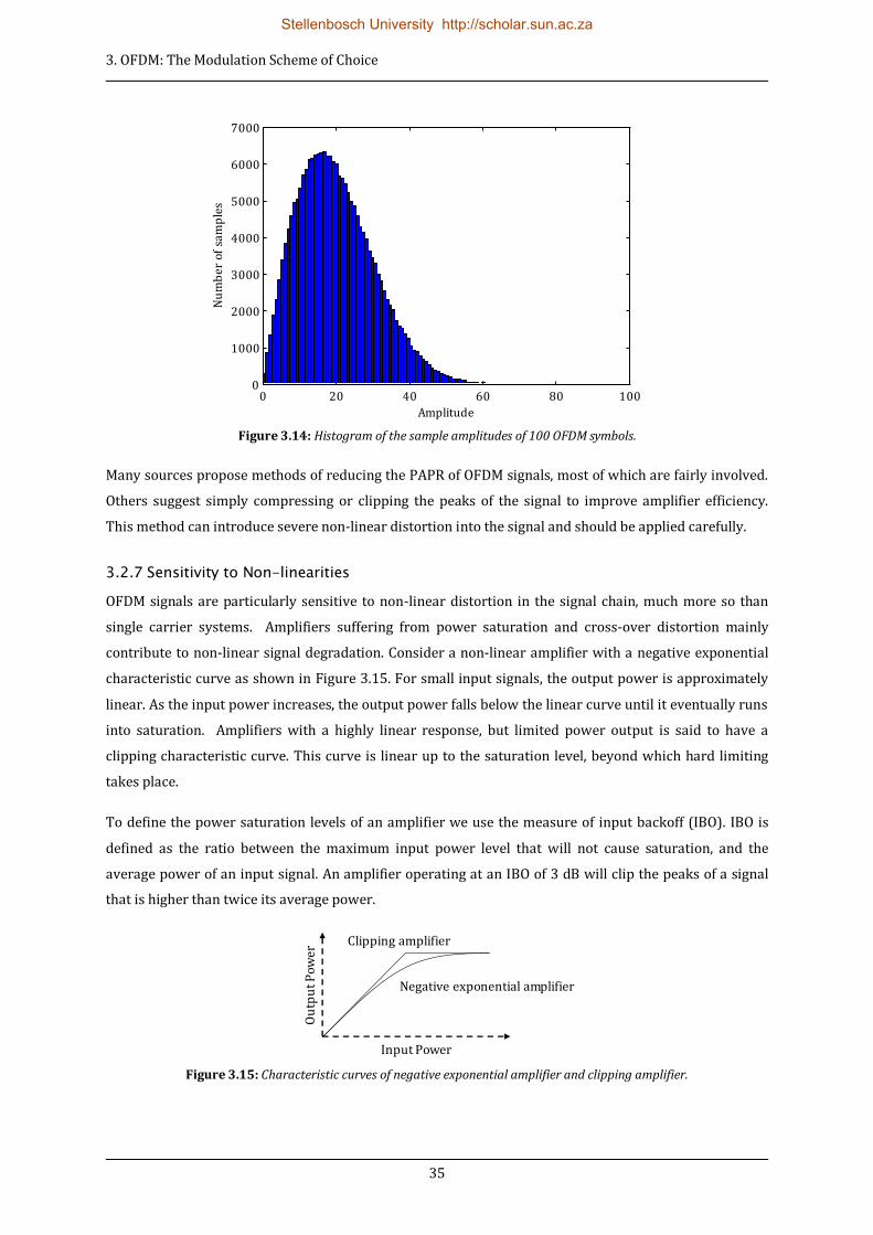
3. OFDM: The Modulation Scheme of Choice
35
Figure 3.14: Histogram of the sample amplitudes of 100 OFDM symbols.
Many sources propose methods of reducing the PAPR of OFDM signals, most of which are fairly involved.
Others suggest simply compressing or clipping the peaks of the signal to improve amplifier efficiency.
This method can introduce severe non-linear distortion into the signal and should be applied carefully.
3.2.7 Sensitivity to Non-linearities
OFDM signals are particularly sensitive to non-linear distortion in the signal chain, much more so than
single carrier systems. Amplifiers suffering from power saturation and cross-over distortion mainly
contribute to non-linear signal degradation. Consider a non-linear amplifier with a negative exponential
characteristic curve as shown in Figure 3.15. For small input signals, the output power is approximately
linear. As the input power increases, the output power falls below the linear curve until it eventually runs
into saturation. Amplifiers with a highly linear response, but limited power output is said to have a
clipping characteristic curve. This curve is linear up to the saturation level, beyond which hard limiting
takes place.
To define the power saturation levels of an amplifier we use the measure of input backoff (IBO). IBO is
defined as the ratio between the maximum input power level that will not cause saturation, and the
average power of an input signal. An amplifier operating at an IBO of 3 dB will clip the peaks of a signal
that is higher than twice its average power.
Figure 3.15: Characteristic curves of negative exponential amplifier and clipping amplifier.
0 20 40 60 80 1000
1000
2000
3000
4000
5000
6000
7000
Amplitude
Nu
mb
er
of s
am
ple
s
Negative exponential amplifier
Clipping amplifier
Input Power
Ou
tpu
t Pow
er
Stellenbosch University http://scholar.sun.ac.za

3. OFDM: The Modulation Scheme of Choice
36
Non-linearities can severely influence the frequency response of an OFDM signal. The higher order mixing
products introduced by non-linearities cause harmonic distortions of every subcarrier in the signal. The
harmonic components interfere additively with the useful signal so that every subcarrier is essentially
affected by the mixing products of many other subcarriers. Based on the central limit theory, we expect
the additive interference caused by many random processes to behave as a Gaussian random variable. We
can thus model distortion due to non-linearities in the signal chain as additive white Gaussian noise.
Figure 3.16 shows the QAM constellation of an OFDM signal with and that is clipped
at an IBO of 6 dB. Additive white Gaussian noise is evident in the distributions of the symbols. The
resulting signal-to-interference ratio (SIR) is about 30 dB. It is arguable that the interference from non-
linear distortion can be ignored if the SIR is sufficiently larger than the expected SNR of the channel. If the
characteristic curve of an amplifier is known, non-linearities can be remedied by pre-distorting the signal
before amplification.
Figure 3.16: QAM constellation of OFDM signal clipped at an IBO of 6 dB.
3.3 Applying OFDM to the Underwater Environment
From the previous section we can conclude that multicarrier modulation and more specifically OFDM is a
very well suited modulation scheme for the underwater environment. Our discussion up to now has been
from a general perspective, so that no mention has been made of how OFDM should be applied to the
underwater channel. In this section we combine our knowledge of the underwater channel and the
principles of orthogonal multicarrier modulation to design a practical OFDM signal that will perform well
for an underwater modem.
3.3.1 Pass Band Modulation
The absorption of acoustic energy in salt water increases proportionally with frequency. From Figure 2.5
we expect about 10 dB attenuation per kilometre at a carrier frequency of 50 kHz. Beyond 50 kHz the
attenuation increases rapidly. In order for a communication link to cover a reasonable distance without
-4 -2 0 2 4
-4
-2
0
2
4
Stellenbosch University http://scholar.sun.ac.za

3. OFDM: The Modulation Scheme of Choice
37
excessive attenuation, the operating frequency should be chosen as low as possible while still providing
adequate data rates.
The typical OFDM transmitter shown in Figure 3.7 uses a quadrature modulator to convert the complex
baseband OFDM signal into a real passband signal that can be transmitted. Radio frequency systems with
relatively high centre frequencies generally use this method of passband modulation. However, a
quadrature modulator significantly increases the complexity of the analogue design. For centre
frequencies well below the capabilities of modern high speed DAC’s and ADC’s it would be preferable to
complete the passband modulation in software.
It follows from signal processing theory that a real periodic time signal can be expressed as a Fourier
series represented by the sum of harmonic sine and cosine signals. In the frequency domain cosine
signals have real even symmetry and sine signals have complex odd symmetry about the axis [10].
From this we can deduce that the Fourier analysis of a real time signal will have complex conjugate
symmetry about the axis. By following the inverse of this argument we can directly generate a real
discrete time domain signal from the Fourier synthesis by adapting the composition of the FFT window so
that it possesses complex conjugate symmetry. The sampling frequency should be at least twice the
maximum subcarrier frequency. The coefficients of the FFT window corresponding to the passband
bandwidth are modulated by a block of parallel data symbols. The mirrored complex conjugate of the data
symbols are positioned so that the FFT window is conjugate symmetric about the ⁄ axis. The
remaining coefficients are set to zero. Figure 3.17 shows the construction of the FFT window for a direct-
to-passband Fourier synthesis.
Figure 3.17: Conjugate symmetric FFT window for direct-to-passband Fourier synthesis.
It seems that with a lot of carriers set to zero, the data throughput of the system will suffer. However, it
can be shown that the data rate is not dependant on the number of occupied subcarriers, but only on the
passband bandwidth. Given the sampling frequency and the FFT window size, we can determine the
carrier spacing as
(3.19)
The number of occupied carriers in the passband bandwidth is
Original data carriers Conjugate mirror of data carriers | |k
p
sf
2
sf
f
B
Stellenbosch University http://scholar.sun.ac.za

3. OFDM: The Modulation Scheme of Choice
38
(3.20)
so that the QAM symbol rate is
(3.21)
By substituting equation 3.20 into 3.21 and noting that and are reciprocals, the QAM symbol rate
reduces to
(3.22)
The passband bandwidth is generally limited by the transducers used. These devices have fairly narrow
operating bandwidths although some wideband variants do exist. Chapter 5 provides a detailed
discussion on transducers.
3.3.2 Timing and Frequency Synchronisation
As mentioned in the previous section, timing synchronization of a receiver can be done by including
known OFDM symbols in the transmitted signal. We know that OFDM signals behave similarly to white
noise, so that we can expect very good autocorrelation properties, i.e. impulse like. By cross correlating
the known symbol with the received signal, and implementing a peak detector, near perfect timing
synchronisation can be achieved. By exploiting this concept and including two known symbols per frame
with fixed timings, we should be able to determine the frequency offset between transmitter and receiver.
Not only this, but we can also use the subcarrier amplitude and phase of the known received symbols to
determine the channel response.
We define a frame structure with a fixed length so that data carrying symbols are preceded by a preamble
symbol and followed by a postamble. To generate the amble symbols we need to assign a pseudo random
sequence of symbols to all data carriers. So called pseudo noise (PN) sequence generators are an efficient
method of achieving this. A PN generators produces a random sequence of binary numbers. With slight
numeric manipulation, this sequence can be used as BPSK symbols in the Fourier synthesis of an OFDM
symbol.
A PN generator can be implemented with a shift register and modulo two adders as shown in Figure 3.18.
With each time step the values in the registers is shifted one position to the right and added modulo 2 to
generate the next output value. The value to be entered at the left most register is calculated as a masked
modulo two sum of all the elements in the register. This mask is called the generator polynomial. The first
and last coefficients of the generator polynomial are set to one. The initial state of the registers can be
specified as a binary sequence with a length of one less than the generator polynomial. Some
implementations also use a mask when calculating the output value.
Stellenbosch University http://scholar.sun.ac.za

3. OFDM: The Modulation Scheme of Choice
39
Figure 3.18: PN generator by shift register implementation.
To convert the binary output sequence to BPSK symbols we simply multiply it by two and subtract one.
Some experimentation with different generator polynomials and initial states is necessary to find two
sufficiently random sequences that yield OFDM symbols with excellent autocorrelation properties. The
cross-correlation of a preamble and postamble with a null frame is shown in Figure 3.19. Note the
impulse like autocorrelation.
Figure 3.19: Cross-correlation of preamble and postamble with null frame.
From signal processing theory we know that correlation and convolution is similar processes in the time
domain. Thus we expect the correlation to show modulated sinc impulse-like characteristics. In order to
accurately determine the centre of the impulse we devise an algorithm that essentially performs envelope
detection. We start off by up-sampling the portion of the correlation that contains the detected peak to
improve resolution. Next we rectify the up-sampled correlation to facilitate envelope detection. The local
maximum of each period of the modulated sinc are identified as points that lie on the envelope. The
envelope is calculated by fitting a cubic spline through all local maxima. The highest point on the envelope
coincides with the centre of the sinc impulse. Figure 3.20 illustrates the peak detection process. The
reader should note that the maximum sample value does not always coincide with the centre of the peak
as is the case is in the Figure. A phase offset of the received signal can shift the peak to a position between
local maxima.
0g
1g
2ng
1ng
ng
Output
1nr
nr2
r0
0 2000 4000 6000 8000 10000-1
-0.5
0
0.5
1
Sample values
No
rma
lised
am
pli
tud
e
Preamble
Postamble
Stellenbosch University http://scholar.sun.ac.za

3. OFDM: The Modulation Scheme of Choice
40
Figure 3.20: Peak detection by envelope detection.
With this method of peak detection we can determine the length of a frame with single sample accuracy. A
frequency offset whether due to a sample rate mismatch or Doppler shift will prolong or shorten the
received frame. The frame length can be corrected by the process of sample rate conversion. Likewise,
sample rate conversion can also be used to simulate Doppler shift in a theoretical channel model. The
process essentially involves interpolating between samples of the received signal and selecting new
sample values from the interpolation curve at the desired rate.
A general algorithm for sample rate conversion calculates the lowest common multiple of the original and
desired sample rate and up-samples the original signal to this rate by zero-padding each sample. A
reconstruction filter with a finite impulse response, usually in the form of a truncated sinc function, is
used to ‘fill-in’ the zeros in the up-sampled signal. The signal is then down-sampled by only selecting
those sample values that coincide with the desired sample rate. In order to improve computational
efficiency, polyphase decompositioning is used to calculate only the sample values in the up-sampled
signal that will feature in the desired resampled signal. The truncated sinc impulse is placed at the
desired sample instance. The values of the sinc at the original sample instances are used as coefficients for
the weighted summation of the original sample values to calculate the desired sample value. Figure 3.21
shows a graphical representation of sample rate conversion by polyphase decompositioning.
Figure 3.21: Sample rate conversion by polyphase decompositioning. Blue indicates the resampled signal values.
MATLAB has a built-in resample function that uses a polyphase filter implementation, but sets a
limitation on the lowest common multiple of the up-sampling and down-sampling factors at
. Consider an original frame of 50 000 samples, and that we can detect the peak of the correlation with
2020 2030 2040 2050 2060 2070 20800
0.2
0.4
0.6
0.8
1
1.2
1.4
Time t [sample index]
Am
pli
tud
e
Cross correlation
Upsampled correlation
Envelope
Peak
Threshold
t
Stellenbosch University http://scholar.sun.ac.za
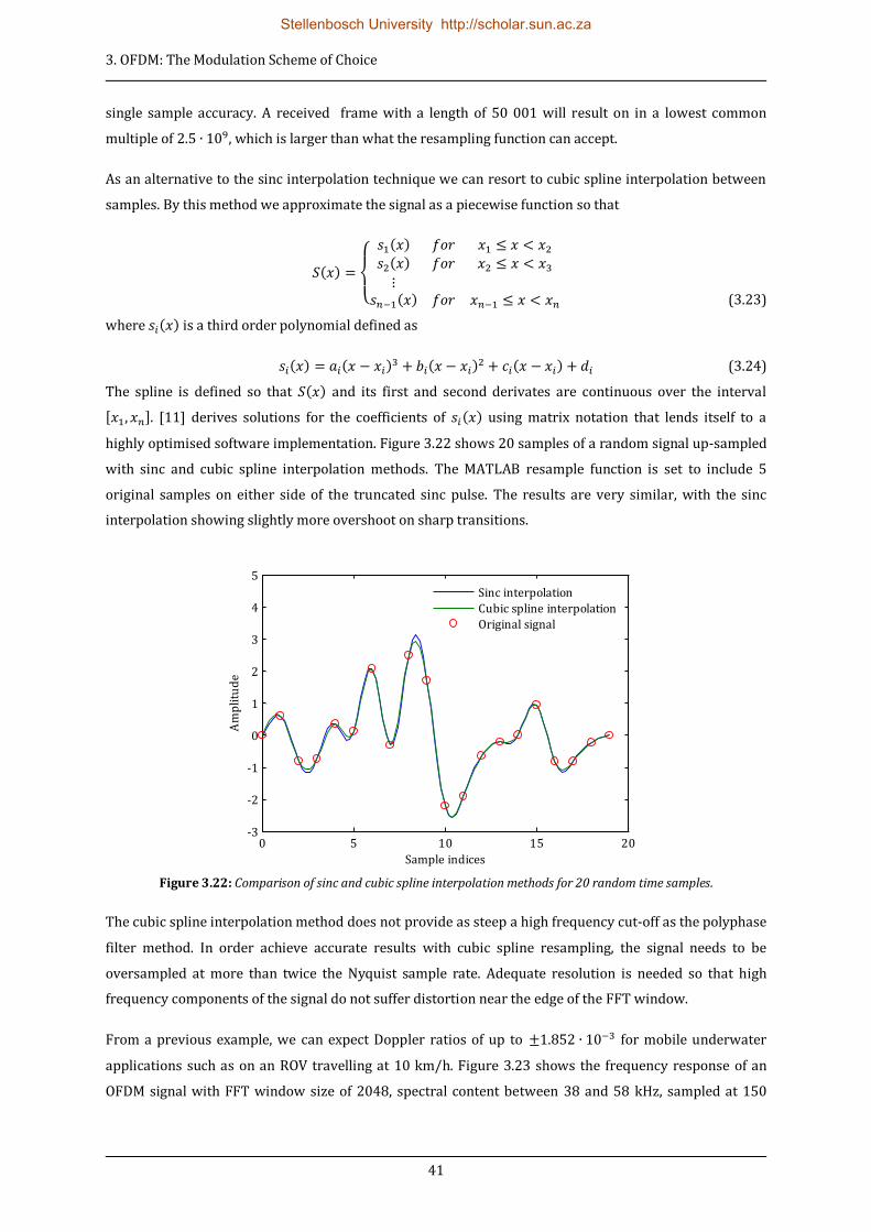
3. OFDM: The Modulation Scheme of Choice
41
single sample accuracy. A received frame with a length of 50 001 will result on in a lowest common
multiple of , which is larger than what the resampling function can accept.
As an alternative to the sinc interpolation technique we can resort to cubic spline interpolation between
samples. By this method we approximate the signal as a piecewise function so that
( )
( )
( )
( )
(3.23)
where ( ) is a third order polynomial defined as
( ) ( ) ( )
( ) (3.24)
The spline is defined so that ( ) and its first and second derivates are continuous over the interval
[ ]. [11] derives solutions for the coefficients of ( ) using matrix notation that lends itself to a
highly optimised software implementation. Figure 3.22 shows 20 samples of a random signal up-sampled
with sinc and cubic spline interpolation methods. The MATLAB resample function is set to include 5
original samples on either side of the truncated sinc pulse. The results are very similar, with the sinc
interpolation showing slightly more overshoot on sharp transitions.
Figure 3.22: Comparison of sinc and cubic spline interpolation methods for 20 random time samples.
The cubic spline interpolation method does not provide as steep a high frequency cut-off as the polyphase
filter method. In order achieve accurate results with cubic spline resampling, the signal needs to be
oversampled at more than twice the Nyquist sample rate. Adequate resolution is needed so that high
frequency components of the signal do not suffer distortion near the edge of the FFT window.
From a previous example, we can expect Doppler ratios of up to for mobile underwater
applications such as on an ROV travelling at 10 km/h. Figure 3.23 shows the frequency response of an
OFDM signal with FFT window size of 2048, spectral content between 38 and 58 kHz, sampled at 150
0 5 10 15 20-3
-2
-1
0
1
2
3
4
5
Sample indices
Am
pli
tud
e
Sinc interpolation
Cubic spline interpolation
Original signal
Stellenbosch University http://scholar.sun.ac.za

3. OFDM: The Modulation Scheme of Choice
42
kHz. The signal was Doppler shifted with a ratio of and then corrected with cubic spline
interpolation. Edge effect distortion and the gradual cut-off slope are clearly visible.
Figure 3.23: Frequency response of Doppler corrected OFDM signal with inadequate oversampling for sample rate
conversion by cubic spline interpolation.
We expect the Doppler shift to also influence the correlation properties of the pre- and postambles so that
the peaks become less pronounced. Figure 3.24 shows the normalized correlation of an original and a
Doppler shifted preamble with ratio of . At this ratio the cross-correlation has a peak
amplitude of half the autocorrelation. This number is somewhat dependant on the sample rate and FFT
window size and should be experimented with based on the specific signal parameters.
Figure 3.24: Correlation of original preamble and Doppler shifted preamble with ratio of .
0 50 100 1500
0.2
0.4
0.6
0.8
1
Frequency f [kHz]
Am
pli
tud
e
0 2000 4000 6000 8000 10000-1
-0.5
0
0.5
1
Time t [sample index]
No
rma
lised
am
pli
tud
e
Original preamble
Resampled preamble
Stellenbosch University http://scholar.sun.ac.za

3. OFDM: The Modulation Scheme of Choice
43
3.3.3 Channel Estimation
Efficient channel estimation is essential for coherent demodulation of an OFDM signal. The art of channel
estimation lies therein to find a compromise between channel predicting ability and computational
complexity. We can view an OFDM signal as a two dimensional lattice in the time-frequency plane. Cells in
the frequency dimension are occupied by subcarriers. These are modulated in the time dimension by
different symbols. Subcarriers modulated with known symbols serve as pilot carriers. Figure 3.25 shows
three basic pilot carrier arrangements. The purpose of channel estimation is to characterise the expected
influence of the channel on data carriers at positions between pilot carriers. Estimation can be based in
either the time or frequency dimensions or both. One-dimensional estimation is significantly less
complex, while estimation in two dimensions provides much better channel tracking performance. The
optimal channel estimator is based on two-dimensional Wiener filter interpolation, but this technique
possesses a very high level of complexity. In general, one-dimensional estimation is implemented in
OFDM systems to provide a good trade-off between accuracy and complexity.
Figure 3.25: Block, comb and interleaved pilot arrangements. Solid cells indicate pilots, blank cells indicate data
carriers.
One-dimensional estimation techniques are based on block- and comb-type pilot arrangements. Block
arrangements fare well in slow fading channels where the frequency response changes slowly with time,
but varies significantly in the frequency dimension. For fast fading channels, where the response can vary
appreciably from one symbol to the next, a comb-type arrangement will perform best. Interleaved
arrangements provide a combination of block and comb arrangements and are generally used in two-
dimensional estimation. The interleaving strategy will depend on the channel properties.
To determine which arrangement is optimal for the underwater channel, we revisit some of the channel
properties discussed in Chapter 2. The coherence bandwidth of a communication channel is a statistical
measure of the maximum bandwidth for which different frequency components of a signal will
experience similar of correlated fading. It is inversely proportional to the delay spread of the channel.
With a large delay spread, the expected coherence bandwidth of the underwater channel is very narrow.
For OFDM signals with subcarrier spaced wider apart than the coherence bandwidth, we expect the
subcarriers to experience uncorrelated fading in the frequency dimension. This condition renders any
attempt at interpolation between sparse pilot positions in the frequency dimension futile. Pilots at all
subcarrier positions are needed to accurately determine the channel response.
time
freq
uen
cy
time
freq
uen
cy
time
freq
uen
cy
Stellenbosch University http://scholar.sun.ac.za

3. OFDM: The Modulation Scheme of Choice
44
The coherence time of a communication channel is a statistical measure of the time duration for which
the channel can be considered time invariant. It is inversely proportional to the Doppler spread of the
channel. For slow moving mobile applications operating at low centre frequencies, we expect the Doppler
spread to be small so that the coherence time is long. This results in a slow fading channel. If the pilot
spacing in the time dimension is sufficiently dense, so that their intervals are of the same order as the
coherence time, interpolation between pilot positions in the time dimension is possible. We can deduce
that a block-type pilot arrangement is in fact the optimal arrangement for channel estimation in the
underwater environment. Our method of including a preamble and postamble for timing and frequency
synchronisation, as discussed in the previous subsection, essentially follows a block arrangement. The
number of data carrying symbols between ambles, i.e. the frame length, will ultimately be determined by
the coherence time of the channel.
One-dimensional estimation techniques based on block arrangements include least square (LS), minimum
mean square error (MMSE) and modified MMSE. LS estimators provide the lowest complexity without
employing any statistical knowledge of the channel in the estimation process. MMSE estimators use
statistical knowledge in the form of the autocovariance of the channel to minimise the mean square error.
It provides better performance than LS estimators, but has very high computational complexity,
especially for large numbers of carriers since it involves a number of matrix inversions for each pilot
block. Modified MMSE estimators attempt to reduce complexity by employing various approximations
and methods of simplification.
As an initial effort we choose a modified LS estimator due to its simplicity. The task at hand is to estimate
the channel coefficients denoted by vector , given the transmitted pilot symbols as the diagonal matrix
and the received symbols as a vector . The squared error parameter to minimise is given by
( )
( ) (3.25)
where ( ) denotes the conjugate transpose of . [12] shows that the least square estimate of is given
by
[
⁄ ]
(3.26)
The LS estimated channel is simply the quotient of the transmitted pilot symbols and the received
symbols. Since our frame structure is defined to include a preamble and postamble, we have two sets of
pilot blocks available for the channel estimation of each frame. We expect the channel to show some
degree of time variance, so that the estimates obtained from the preamble and postamble will differ. By
defining the frame length so that the time variance over it can be approximated as linear, we can
interpolate between estimates at the preamble and postamble positions. The channel response used to
correct the data carrying symbols will thus be a linear combination of the estimates at the preamble and
postamble positions.
Stellenbosch University http://scholar.sun.ac.za

3. OFDM: The Modulation Scheme of Choice
45
3.3.4 QAM Constellations
An important aspect of OFDM modulation is the choice of constellation diagram. We have mentioned that
each QAM symbol corresponds to a bit sequence from the serial message bit stream. The symbols can be
represented by complex vectors with a certain amplitude and phase angle, or equivalently a real and
imaginary component. In signal processing, these are often referred to as the in-phase and quadrature
components.
A constellation diagram essentially divides the complex signal space into a number of regions. At the
centre point of each region lies a QAM symbol. At the transmitter, symbols are drawn from the
constellation diagram to serve as coefficients in the FFT synthesis of the OFDM signal. The symbols
effectively modulate the amplitude and phase of the complex subcarriers. At the receiver, demodulated
symbols will be scattered about their original positions due to distortions along the signal path. The
performance of the receiver will be determined by its ability to discern between symbols from different
regions. A constellation with many closely spaced symbols will be much more sensitive to distortions
than a simple constellation with fewer sparse symbols. However, fewer symbols means that the number
of unique bit sequences that can be represented decreases. For a given number of symbols , the length
of the bit sequence per symbol is the largest integer so that
(3.27)
Two variants of constellations are generally used. If all symbols have equal amplitude and differ only in
phase, it is referred to as phase shift keying (PSK). If the amplitude and phase are varied, it is known as
quadrature amplitude modulation (QAM). A number of popular PSK and QAM constellation diagrams are
shown in Figure 3.26.
Figure 3.26: Popular PSK and QAM constellation diagrams.
1
8-PSK 16-QAM
BPSK QPSK
1
1
4
1
Stellenbosch University http://scholar.sun.ac.za

3. OFDM: The Modulation Scheme of Choice
46
These diagrams all possess simple symmetry which facilitates efficient decoding. The regular
arrangement of the symbols allows for easy implementation of the decoding decisions by simply
evaluating the phase or real and imaginary values. For example, if a received QPSK symbol has a phase
between –
and
, then it represents the bit sequence 00 and so forth. Although these regular
symmetrical arrangements lend themselves toward efficient decoding, they will not always deliver the
lowest possible symbol error rate. By optimising the arrangement so that symbols occupy the
constellation more densely while maintaining the distance between adjacent symbols, we can improve
the symbol error rate for a given SNR. Think of it as a way to lower the average signal power, without an
increase in symbol error rate, while the noise power remains fixed.
As a Figure of merit (FOM) to compare the optimality of different constellation diagrams we can use the
ratio between the average power of the constellation and the minimum noise power that will cause a
symbol error. With hard decision decoding a symbol will be decoded as the original symbol to which it
lies closest so that the minimum noise power for a symbol error is half the distance between adjacent
symbols squared. We present this mathematically as
∑| |
(
)
⁄ (3.28)
with the amplitude of the mth symbol and the distance between adjacent symbols. For a given
number of symbols in a constellation, we want the Figure of merit to be a small as possible. It can be
shown that the FOM for BPSK and QPSK constellations is 1 and 2 respectively. These constellations
already possess optimal arrangements.
For eight-symbol constellations we are left with a choice between QAM and PSK. 8-PSK and rectangular 8-
QAM can be decoded fairly efficiently, but they do not present optimal arrangements. We determine the
FOM for the 8-PSK constellation, as shown in Figure 3.27, as
( (
⁄ )
)
(3.29)
The FOM for rectangular 8-QAM is
( ( ) ( ))
(3.30)
The optimal 8-QAM constellation with the lowest possible FOM is shown in Figure 3.27. Its FOM is
( ( ) ( √ )
)
(3.31)
Stellenbosch University http://scholar.sun.ac.za
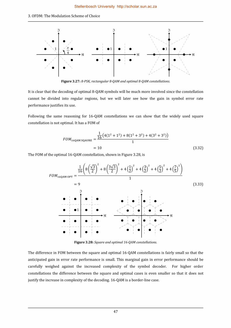
3. OFDM: The Modulation Scheme of Choice
47
Figure 3.27: 8-PSK, rectangular 8-QAM and optimal 8-QAM constellations.
It is clear that the decoding of optimal 8-QAM symbols will be much more involved since the constellation
cannot be divided into regular regions, but we will later see how the gain in symbol error rate
performance justifies its use.
Following the same reasoning for 16-QAM constellations we can show that the widely used square
constellation is not optimal. It has a FOM of
( ( ) ( ) ( ))
(3.32)
The FOM of the optimal 16-QAM constellation, shown in Figure 3.28, is
( (√
)
( √
)
( )
( )
( )
( )
)
(3.33)
Figure 3.28: Square and optimal 16-QAM constellations.
The difference in FOM between the square and optimal 16-QAM constellations is fairly small so that the
anticipated gain in error rate performance is small. This marginal gain in error performance should be
carefully weighed against the increased complexity of the symbol decoder. For higher order
constellations the difference between the square and optimal cases is even smaller so that it does not
justify the increase in complexity of the decoding. 16-QAM is a border-line case.
1
4
1
1
1
Stellenbosch University http://scholar.sun.ac.za

3. OFDM: The Modulation Scheme of Choice
48
3.3.5 Symbol Error Probabilities
The Figure of merit concept provides a simple way of comparing the anticipated performance of
constellation diagrams. However, to assess the reliability of a communication link we need to determine
the anticipated symbol probabilities for given noise levels.
By assuming that all signal distortions behave as additive white Gaussian noise, we expect the probability
density functions of the demodulated symbols to obey a Gaussian distribution. In order to determine the
probability of a symbol error we have to integrate the two dimensional distribution function over the
region for which a symbol will be erroneously decoded. Alternatively we can integrate the distribution
over the region for which a symbol will be correctly decode and subtract it form one.
3.3.5.1 Regularly Arranged Constellations
For regularly arranged constellations, with symbol boundaries that are parallel to the real or imaginary
axis, the task is fairly simple. We start off by defining error probabilities for symbols in a single dimension
and later expand it to include the real and imaginary components.
The probability density function for additive white Gaussian noise is
( )
√
( )
(3.34)
with the mean and the variance. We define a reference symbol as the symbol located at the origin.
Additive noise with power
, will scatter received symbols about reference symbol so that the
mean is zero. The region for which the reference symbol will be correctly decoded can be bounded in two
ways, in any particular dimension, i.e. real or imaginary. Figure 3.29 shows the reference symbol bounded
by a single boundary and a double boundary. Its distance from the boundary is defined as .
Figure 3.29: Singularly and doubly bounded reference symbols.
For the singularly bounded scenario we have that a received symbol will be correctly decoded if its
component in the corresponding dimension is larger than . The probability can be written as
( | ) ( )
√
∫
(3.35)
We substitute the exponent with so that
√
(3.36)
The limits of the integral becomes
d d d
( , )0 0 ( , )0 0
Stellenbosch University http://scholar.sun.ac.za

3. OFDM: The Modulation Scheme of Choice
49
√
(3.37)
√
(3.38)
and the derivative becomes
√
√ (3.39)
The probability reduces to
( | )
√ ∫
√
(
√
) (3.40)
with ( ) defined as
( )
√ ∫
(3.41)
From the symmetry of the erfc function it follows that
( ) ( ) (3.42)
So that
( | )
(
√
) (3.43)
For a doubly bounded reference symbol we can write
( | ) ( )
√
∫
(3.44)
Note that the integral can be rewritten as a difference of two integrals so that
( | )
√
[∫
∫
] (3.45)
By making the same substitution as in equation 3.31, the probability reduces to
( | )
(
√
)
(
√
) (3.46)
Again applying the symmetry of the erfc function the probability becomes
Stellenbosch University http://scholar.sun.ac.za

3. OFDM: The Modulation Scheme of Choice
50
( | )
( (
√
))
(
√
)
(
√
) (3.47)
Additive white Gaussian noise will have uncorrelated real and imaginary components so that the
probabilities in different dimension can simply be multiplied to determine the resulting probability.
Consider a symbol bounded in the real dimension at – and and in the imaginary dimension at – . Its
correct probability will be
( | ) ( )
( ) ( )
( | ) ( | )
( (
√
))(
(
√
))
(3.48)
By following the same logic we derive the error probabilities for all possible combinations of bounding as
( | )
(
√
) (3.49)
( | ) (
√
) (3.50)
( | ) (
(
√
))
(3.51)
( | ) ( (
√
))(
(
√
))
(3.52)
( | ) ( (
√
))
(3.53)
Any square QAM constellation can be build from these bounded symbols. Assuming equiprobable
symbols, we determine the total symbol error probability as
( ) ∑ ( | ) ( )
(3.54)
To determine the correct probability for a given SNR we express the average energy of all the symbols
in terms of and set it as the subject so that
d
d d
d
d
d
d
d
d
Stellenbosch University http://scholar.sun.ac.za

3. OFDM: The Modulation Scheme of Choice
51
∑| |
√
(3.55)
For illustration we determine the correct probability of BPSK as
( | )
(
(
√
))
(
(
√
))
(
√
) (3.56)
For BPSK we determine the average signal energy as
( )
√ (3.57)
By substituting this we can express the probability in terms of the SNR
( | )
(√
)
(3.58)
The symbol error probability in terms of the SNR is thus
( | ) ( | )
(√
)
(3.59)
Following the same logic we can show that the symbol error probability for higher order constellations is
( | ) (√
)
(√
)
(3.60)
( | )
(√
)
(√
)
(3.61)
( | )
(√
)
(√
)
(3.62)
Plots of symbol error rates versus SNR for the different constellations are shown in Figure 3.30.
Stellenbosch University http://scholar.sun.ac.za

3. OFDM: The Modulation Scheme of Choice
52
3.3.5.2 Irregularly Arranged Constellations
The error boundaries between symbols on the optimised 8-QAM and 16-QAM constellation do not lend
themselves toward simple integration over the enclosed regions. Analytic methods of determining the
symbol error probabilities are fairly involved, so that we rather resort to simulation to determine these.
The results of a simulation that draws equiprobable random symbols form an optimised
constellation and adding white Gaussian noise to it, is shown in Figure 3.30. The additive noise power is
specified so that the resulting SNR increases with increments of 0.5 dB.
Figure 3.30: Symbol error probabilities versus SNR of different constellations.
Note that optimal 8-QAM outperforms rectangular 8-QAM by a margin of slightly more than 1 dB for any
given symbol error probability. The performance difference between square and optimal 16-QAM is very
small, so that in practical systems it will barely be noticeable. Symbol error probabilities are also often
expressed as a function of energy per bit so that ( ) .
3.3.6 Bit Error Probabilities
With the symbol error rates known, we can advance to determining the bit error probabilities. The
expected bit error rate will determine the strength of the error correction coding needed to provide
reliable communication over a noisy channel. Each symbol on a constellation represents a certain bit
sequence. An erroneously detected symbol will be decoded as a different bit sequence. The allocation of
bit sequences to symbols should be optimised so that a symbol error causes as few as possible bit errors.
Gray-coding assigns bit sequences to symbols in such a way that adjacent symbols differ only in one bit.
Such combinations are said to have a Hamming distance of 1. Figure 3.31 shows a square 16-QAM
constellation with Gray coding.
4 6 8 10 12 14 16 18 20 2210
-6
10-5
10-4
10-3
10-2
10-1
Sym
bo
l err
or
pro
ba
bil
ity
SNR Es/N
0 [dB]
BPSKQPSK
Optimal 8-QAM
Rectagular 8-QAM
Optimal 16-QAMSquare 16-QAM
Stellenbosch University http://scholar.sun.ac.za

3. OFDM: The Modulation Scheme of Choice
53
Figure 3.31: Gray coded 16-QAM constellation.
For additive noise levels that are relatively low, we can assume that erroneous symbols will fall to directly
adjacent symbols. For Gray coded constellations this will result in a single bit error per symbol error. We
can approximate the bit error probability for low noise as
( )
( | )
(3.63)
For optimized constellation diagrams, Gray coding is not always possible if the number of directly
adjacent symbols is more than the length of the bit sequence per symbol. By efficiently assigning bit
sequences to symbols it should be possible for most adjoining symbols to have a Hamming distance of 1,
while as few as possible should have a Hamming distance of 2. The bit error probability for a given
symbol error probability becomes more complicated to determine. Consider the optimal 8-QAM
constellation with bit sequences assigned as shown in Figure 3.32.
Figure 3.32: Bit sequence assignment to optimal 8-QAM constellation
with Hamming distance indicated with single or double dashes.
Let be the number of symbols transmitted, so that the number of bits is . The symbol error rate is
(3.64)
and the bit error rate is
(3.65)
We want to express the bit error probability as a function of symbol error probability so that
011
010
110 101
001
111
000
100
Stellenbosch University http://scholar.sun.ac.za

3. OFDM: The Modulation Scheme of Choice
54
( ) ( )
(3.66)
then
(3.67)
We essentially want to determine how many bit errors will occur given that a symbol error has occurred.
We can assume that symbol errors across all boundaries are equally likely. There are twelve possible
boundaries that a symbol can cross to be erroneously decoded, 4 of which cause double bit errors and 8
that cause single bit errors. Let us assume 12 symbol errors have occurred, each across a different
boundary, so that there are 36 bits is question. The number of bit errors is
(3.68)
The ratio of bit errors to symbol errors is thus ⁄ . This gives
( | )
( ) (3.69)
We can express the general relation between bit error probability and symbol error probability as
( )
( )
(3.70)
denotes the sum of the bit errors across boundaries and the number of boundaries between adjacent
symbols. For optimal 16-QAM we have
( | )
( ) (3.71)
At first sight, the assumption of equiprobable boundary crossings seems counterintuitive, but the reader
should note that we are no longer considering symbol error probabilities. We have a given symbol error,
so that this error could have occurred for any symbol across any boundary with equal likelihood. This
result has been confirmed by extensive simulations. Reassigning bit sequences, so that the positions of
double bit errors are different, has no influence on the result.
A comparison of the bit error probabilities of different constellations are shown in Figure 3.33.
Stellenbosch University http://scholar.sun.ac.za

3. OFDM: The Modulation Scheme of Choice
55
Figure 3.33: Bit error probabilities versus SNR of different constellations.
We see that even though optimal 8-QAM has more bit errors per symbol error it outperforms rectangular
8-QAM by a gain margin of 1 dB in SNR for a given bit error rate. The bit error performance of optimal 16-
QAM is almost the same as for square 16-QAM. Any difference will barely be noticeable in a practical
system. However, in an environment where no improvement in performance is too small, we decide to
employ the optimal constellation in the modulation scheme. The modem will operate at relatively low
symbol rates, so that the increased complexity of the decoding algorithm should not be problematic.
3.3.7 Forward Error Correction and Interleaving
The transmission of data across a noisy communications channel will inevitably cause a loss in reliability
of the received data. Bit errors are introduced into the data by erroneously decoded symbols. The
inclusion of redundancy in the transmitted data provides a means of controlling errors. Redundant
symbols are generated and included with the data according to the specifications of a forward error
correction (FEC) code. At the receiver, the decoder uses the redundancy to detect and possibly correct a
limited number of errors without the need for retransmission. The implementation of error coding is
fairly involved so that we will only motivate the choice of a suitable FEC scheme and resort to existing
software libraries to implement it.
FEC codes can be categorised as either block codes or convolution codes. Block coding techniques use a
fixed set of codewords to represent a fixed number of message symbols. Each codeword is treated
independently, so that the block encoder is a memoryless device. Convolution codes process symbol
streams of an arbitrary length adding redundancy that is not only dependant on the current set of input
symbols but on previous symbols as well.
For communication protocols that use fixed frames lengths with a predetermined data capacity, block
codes are usually the most suitable option. Various block codes exist, of which the most popular is
Hamming, Bose-Chaudhuri-Hocquenghem (BCH), and Reed-Solomon codes. These are all families of
4 6 8 10 12 14 16 18 20 2210
-6
10-5
10-4
10-3
10-2
10-1
Bit
err
or
pro
ba
bil
ity
SNR Es/N
0 [dB]
BPSKQPSK
Optimal 8-QAM
Rectagular 8-QAM
Optimal 16-QAMSquare 16-QAM
Stellenbosch University http://scholar.sun.ac.za

3. OFDM: The Modulation Scheme of Choice
56
linear block codes. BCH codes are able to correct multiple errors in binary codewords. The Reed-Solomon
codes are a special class of BCH codes that encode multi-bit symbols and are able to correct multiple burst
errors. Hamming codes are also a subclass of BCH codes that can only correct a single binary error per
codeword. Another family of highly efficient block codes is low-density parity-check (LDPC) codes. With
very long codewords LDPC codes can closely approach the theoretical maximum channel capacity as
proposed by Shannon, but their implementation is significantly more complex.
As with channel estimation the challenge of specifying a suitable FEC code rests on the trade-off between
efficiency and complexity. The efficiency of a code can be interpreted as the amount of redundancy that
must added to the message in order for a receiver to reliably decode the original message given that a
number of errors may have occurred. While LDPC codes provide very high efficiency, their
implementation is severely complex. Hamming codes are relatively simple to implement, but their lacking
ability to correct multiple errors per codeword drastically limit their efficiency. On the contrary, Reed-
Solomon codes offer the correction of multiple burst errors. However, for OFDM signals with their
parallel frequency transmission and low serial symbol rates we do not expect bursts of interference to
affect sequences of contiguous symbols. BCH codes offer multiple bit-corrections per codeword at
moderate complexity and it lends itself to an efficient, yet simple interleaving scheme. While Reed-
Solomon codes could provide similar or even slightly improved performance, we opt for a BCH code as an
initial effort.
BCH codes are specified by two parameters namely the length of the codeword and the number of data
bits per codeword , so that is less than . A specific code is denoted as ( ) is defined so that
(3.72)
with an arbitrary integer larger than two. Valid choices for depends on the degree of the generator
polynomial used in the encoding process. The maximum number of bit errors that can be corrected
depend on the particular code rate. The code rate is defined as the ratio between the codeword length
and the number of data symbols per codeword . For a ( ) code, the code rate is .
The performance of FEC codes exhibit a threshold-effect tendency, whereby the reliability of the decoded
data shows spectacular failure beyond a certain minimum bit error rate. For levels above the threshold,
the decoder can correct all bit errors so that the integrity of the data is preserved. However, below the
threshold, the bit error rate becomes so high that the correctable number or bit-errors is exceeded,
causing the decoder to fail altogether. As a measure of reliability, we can calculate the codeword error
probability. Given the bit error rate, the length of the codeword and the number of correctable bit-errors,
we can set about solving the problem using Bernoulli trails. Each bit in the codeword can be seen an
experiment with only two outcomes: correct or erroneous. A codeword will be erroneously decoded if the
bit-errors exceed the correctable amount. Assuming that bit errors are statically independent with a
probability we can write
Stellenbosch University http://scholar.sun.ac.za

3. OFDM: The Modulation Scheme of Choice
57
( ) ( )
( ) ( ) ( )
∑( )
( )
(3.73)
For long codewords and small bit error probabilities, so that becomes very large and very small, we
can use the Poisson approximation
( )
( )
( )
(3.74)
The probability of an erroneously decoded codeword becomes
( ) ( )
∑( )
(3.75)
Figure 3.34 shows the codeword error probabilities of various BCH codes all with comparable code rates.
For higher bit error probabilities shorter codewords tend to be less error prone than longer ones and vice
versa.
Figure 3.34: Codeword error probabilities of various BCH codes with coding rates between 0.71 and 0.79.
The ultimate measure of the reliability of a communications link is its achievable frame error rate. A
single data frame will generally consist of a number of codewords. If any one of the codewords is
erroneous the entire frame has to be retransmitted. Assuming that codeword errors are statically
independent, we can express the probability of an erroneous frame as
10-3
10-2
10-1
10-6
10-5
10-4
10-3
10-2
10-1
100
Bit error probability
Cod
ew
ord
err
or
pro
bab
ilit
y
BCH(63, 45), t = 3
BCH(127, 99), t = 4
BCH(255, 199), t = 7
BCH(511, 403), t = 12
Stellenbosch University http://scholar.sun.ac.za

3. OFDM: The Modulation Scheme of Choice
58
( ) ( )
( )
( )
( ( ))
(3.76)
with the number of codewords per frame. Figure 3.35 shows the frame error probabilities of the same
BCH codes as in Figure 3.25. The frame length is defined as approximately 511 bits so that it contains one
( ), two ( ), four ( ) or eight ( ) codewords.
Figure 3.35: Error probability for a frame of approximately 511 bits consisting of various numbers of codewords.
To minimise retransmissions we realise that frames consisting of fewer longer codewords will be less
error prone than frames with many short codewords. The ideal approach would be to specify a codeword
length so that a frame contains only a single codeword. However, the length of a code is limited by its
computational complexity. The coding processes of long codewords have especially large memory and
time requirements. Generally codeword lengths are specified to compromise between efficiency and
complexity.
Up to now we have assumed that bit errors occur independently so that errors are equally distributed
across all codewords. The average bit error rate of a communication channel can be misleading in the
sense that bit errors are rarely evenly spread across a frame. In practice we expect burst errors to affect
sequences of contiguous bits, so that some serially transmitted codewords in a frame may contain many
errors while others have none. The frame error rate will suffer considerably even though the FEC codes
were designed to deal with a much higher average bit error rate. Interleaving is a technique devised to
uniformly distribute bit errors across all codewords in a frame. Many methods of interleaving are
commonly employed, but all perform the same basic function of rearranging data in a non-contiguous
way.
10-3
10-2
10-1
10-6
10-5
10-4
10-3
10-2
10-1
100
Bit error probability
Fra
me
err
or
pro
bab
ilit
y
BCH(63, 45), t = 3
BCH(127, 99), t = 4
BCH(255, 199), t = 7
BCH(511, 403), t = 12
Stellenbosch University http://scholar.sun.ac.za
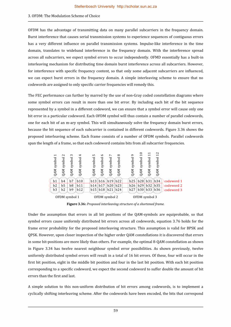
3. OFDM: The Modulation Scheme of Choice
59
OFDM has the advantage of transmitting data on many parallel subcarriers in the frequency domain.
Burst interference that causes serial transmission systems to experience sequences of contiguous errors
has a very different influence on parallel transmission systems. Impulse-like interference in the time
domain, translates to wideband interference in the frequency domain. With the interference spread
across all subcarriers, we expect symbol errors to occur independently. OFMD essentially has a built-in
interleaving mechanism for distributing time domain burst interference across all subcarriers. However,
for interference with specific frequency content, so that only some adjacent subcarriers are influenced,
we can expect burst errors in the frequency domain. A simple interleaving scheme to ensure that no
codewords are assigned to only specific carrier frequencies will remedy this.
The FEC performance can further by marred by the use of non-Gray coded constellation diagrams where
some symbol errors can result in more than one bit error. By including each bit of the bit sequence
represented by a symbol in a different codeword, we can ensure that a symbol error will cause only one
bit error in a particular codeword. Each OFDM symbol will thus contain a number of parallel codewords,
one for each bit of an m-ary symbol. This will simultaneously solve the frequency domain burst errors,
because the bit sequence of each subcarrier is contained in different codewords. Figure 3.36 shows the
proposed interleaving scheme. Each frame consists of a number of OFDM symbols. Parallel codewords
span the length of a frame, so that each codeword contains bits from all subcarrier frequencies.
Figure 3.36: Proposed interleaving structure of a shortened frame.
Under the assumption that errors in all bit positions of the QAM-symbols are equiprobable, so that
symbol errors cause uniformly distributed bit errors across all codewords, equation 3.76 holds for the
frame error probability for the proposed interleaving structure. This assumption is valid for BPSK and
QPSK. However, upon closer inspection of the higher order QAM constellations it is discovered that errors
in some bit-positions are more likely than others. For example, the optimal 8-QAM constellation as shown
in Figure 3.34 has twelve nearest neighbour symbol error possibilities. As shown previously, twelve
uniformly distributed symbol errors will result in a total of 16 bit errors. Of these, four will occur in the
first bit position, eight in the middle bit position and four in the last bit position. With each bit position
corresponding to a specific codeword, we expect the second codeword to suffer double the amount of bit
errors than the first and last.
A simple solution to this non-uniform distribution of bit errors among codewords, is to implement a
cyclically shifting interleaving scheme. After the codewords have been encoded, the bits that correspond
b1
b2 b3
b4
b5 b2
b7
b8 b9
b10
b11 b12
b13
b14 b15
b16
b17 b18
b19
b20 b21
b22
b23 b24
b25
b26 b27
b28
b29 b30
b31
b32 b33
b34
b35 b36
OFDM symbol 1 OFDM symbol 2 OFDM symbol 3
codeword 1
codeword 2
codeword 3
QA
M s
ymb
ol 1
QA
M s
ymb
ol 2
QA
M s
ymb
ol 3
QA
M s
ymb
ol 4
QA
M s
ymb
ol 5
QA
M s
ymb
ol 6
QA
M s
ymb
ol 7
QA
M s
ymb
ol 8
QA
M s
ymb
ol 9
QA
M s
ymb
ol 1
0
QA
M s
ymb
ol 1
1
QA
M s
ymb
ol 1
2
Stellenbosch University http://scholar.sun.ac.za
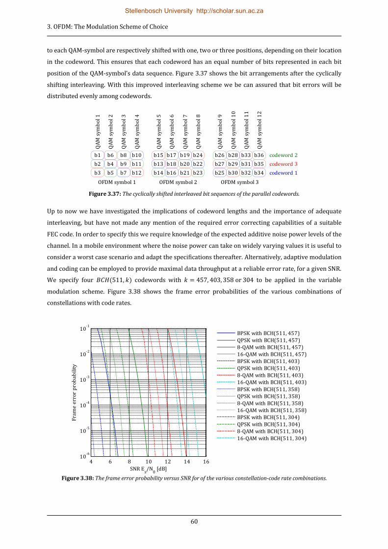
3. OFDM: The Modulation Scheme of Choice
60
to each QAM-symbol are respectively shifted with one, two or three positions, depending on their location
in the codeword. This ensures that each codeword has an equal number of bits represented in each bit
position of the QAM-symbol’s data sequence. Figure 3.37 shows the bit arrangements after the cyclically
shifting interleaving. With this improved interleaving scheme we be can assured that bit errors will be
distributed evenly among codewords.
Figure 3.37: The cyclically shifted interleaved bit sequences of the parallel codewords.
Up to now we have investigated the implications of codeword lengths and the importance of adequate
interleaving, but have not made any mention of the required error correcting capabilities of a suitable
FEC code. In order to specify this we require knowledge of the expected additive noise power levels of the
channel. In a mobile environment where the noise power can take on widely varying values it is useful to
consider a worst case scenario and adapt the specifications thereafter. Alternatively, adaptive modulation
and coding can be employed to provide maximal data throughput at a reliable error rate, for a given SNR.
We specify four ( ) codewords with to be applied in the variable
modulation scheme. Figure 3.38 shows the frame error probabilities of the various combinations of
constellations with code rates.
Figure 3.38: The frame error probability versus SNR for of the various constellation-code rate combinations.
OFDM symbol 1 OFDM symbol 2 OFDM symbol 3
codeword 1
codeword 2
codeword 3
QA
M s
ymb
ol
1
QA
M s
ymb
ol
2
QA
M s
ymb
ol
3
QA
M s
ymb
ol
4
QA
M s
ymb
ol
5
QA
M s
ymb
ol
6
QA
M s
ymb
ol
7
QA
M s
ymb
ol
8
QA
M s
ymb
ol
9
QA
M s
ymb
ol
10
QA
M s
ymb
ol
11
QA
M s
ymb
ol
12
b22
b15
b23
b24 b17
b13
b14
b19
b18 b20
b16 b21
b1 b6
b2
b3
b8
b4
b5
b10
b9 b11
b7 b12 b34
b33 b36
b35
b26
b31
b32
b28
b27 b29
b25 b30
4 6 8 10 12 14 1610
-6
10-5
10-4
10-3
10-2
10-1
Fra
me
err
or
pro
bab
ilit
y
SNR Es/N
0 [dB]
BPSK with BCH(511, 457)
QPSK with BCH(511, 457)
8-QAM with BCH(511, 457)
16-QAM with BCH(511, 457)
BPSK with BCH(511, 403)
QPSK with BCH(511, 403)
8-QAM with BCH(511, 403)
16-QAM with BCH(511, 403)
BPSK with BCH(511, 358)
QPSK with BCH(511, 358)
8-QAM with BCH(511, 358)
16-QAM with BCH(511, 358)
BPSK with BCH(511, 304)
QPSK with BCH(511, 304)
8-QAM with BCH(511, 304)
16-QAM with BCH(511, 304)
Stellenbosch University http://scholar.sun.ac.za

3. OFDM: The Modulation Scheme of Choice
61
Unfortunately, the prototype modem only provides simplex communications so that the variable
modulation scheme cannot be fully implemented. The user is left with choosing the constellation-code
rate combination that will deliver the highest data rate given the specific channel SNR.
3.3.8 Quantisation Resolution
Digital signal processing requires an analogue transmission signal to be sampled and quantised to
discrete time values before processing. Limited quantisation resolution can introduce undesirable errors
into the signal. To evaluate the effects of quantisation on the OFDM signal we follow a statistical approach.
Assuming that the quantisation error is random in nature, we can model it as noise added to the original
signal. As long as the analogue signal falls within the range of the quantiser, so that no clipping occurs, the
error ( ) is bounded in magnitude so that | ( )| ⁄ , where denotes the quantisation step size.
The step size is the quotient of the range of the quantiser and the number of quantisation levels so that
(3.77)
with the number of bits in the binary representation of the quantised value. For our analysis we assume
that ( )is a stationary white noise sequence, uniformly distributed over the range ⁄ ( )
⁄ . This holds given that the quantisation step size is sufficiently small, so that the analogue signal will
traverse several quantisation levels between successive samples. Figure 3.39 shows the probability
density function for the quantisation error.
Figure 3.39: Probability density function of ( ).
For a zero mean and stationary analogue signal, like a typical OFDM signal, we proceed to express the
signal to quantisation noise ratio (SQNR) as
(3.78)
where denotes the signal power and
the additive quantisation noise power. The noise
power can be calculated as
0
( )p e
1
e
2
2
Stellenbosch University http://scholar.sun.ac.za
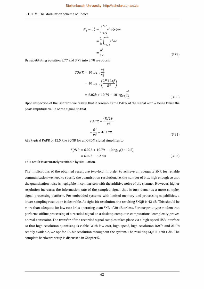
3. OFDM: The Modulation Scheme of Choice
62
∫ ( ) ⁄
⁄
∫
⁄
⁄
(3.79)
By substituting equation 3.77 and 3.79 into 3.78 we obtain
(
)
(3.80)
Upon inspection of the last term we realise that it resembles the PAPR of the signal with being twice the
peak amplitude value of the signal, so that
( )
(3.81)
At a typical PAPR of 12.5, the SQNR for an OFDM signal simplifies to
( )
(3.82)
This result is accurately verifiable by simulation.
The implications of the obtained result are two-fold. In order to achieve an adequate SNR for reliable
communication we need to specify the quantisation resolution, i.e. the number of bits, high enough so that
the quantisation noise is negligible in comparison with the additive noise of the channel. However, higher
resolution increases the information rate of the sampled signal that in turn demands a more complex
signal processing platform. For embedded systems, with limited memory and processing capabilities, a
lower sampling resolution is desirable. At eight-bit resolution, the resulting SNQR is 42 dB. This should be
more than adequate for low rate links operating at an SNR of 20 dB or less. For our prototype modem that
performs offline processing of a recoded signal on a desktop computer, computational complexity proves
no real constraint. The transfer of the recorded signal samples takes place via a high-speed USB interface
so that high-resolution quantising is viable. With low-cost, high-speed, high-resolution DAC’s and ADC’s
readily available, we opt for 16-bit resolution throughout the system. The resulting SQNR is 90.1 dB. The
complete hardware setup is discussed in Chapter 5.
Stellenbosch University http://scholar.sun.ac.za
3. OFDM: The Modulation Scheme of Choice
63
3.4 Summary
In this chapter we conduct an in-depth study of the theory of OFDM and its application to the underwater
environment. We also investigate methods of timing and frequency synchronisation and channel
estimation specifically aimed at OFDM. An extensive study of QAM constellations and their resulting
symbol- and bit error probabilities lead us to optimal arrangements for 8-QAM and 16-QAM
constellations. By combining this with sufficient interleaving and BCH error correcting codes, we are
confident that our proposed OFDM modulation scheme is a sensible solution for acoustic underwater
communications. While this chapter discusses mainly telecommunications theory, the next chapter
focuses on the practical implementation of the knowledge that we have gained here.
Stellenbosch University http://scholar.sun.ac.za

64
4 GENERATING AND DEMODULATING THE SIGNAL
The strength of a software defined modem lies in its simple reconfigurability. A powerful high-level
programming language such as MATLAB is ideal for experimenting with different configurations to aid in
the development of a prototype modem. Apart from its elegantly expressed matrix operations, the strong
suit of MATLAB lies in its powerful built-in libraries. Together with its efficient graphical representation
of data, MATLAB provides an appropriate platform for the development of prototype algorithms. Seeing
that most of the signal processing of this project is done off-line on a desktop computer, MATLAB is well
suited for the design of the modulation and demodulation algorithms.
In the previous chapter we motivate many of the design choices of a practicable OFDM system for
underwater communication, but the discussion remains somewhat removed from the actual
implementation. In this chapter we discuss the particulars of the signal design and also take an in-depth
look at the modulation and demodulation processes.
4.1 Signal Parameters
The physical properties of an OFDM signal are defined by a set of specifications that we refer to as the
signal parameters. Most of these parameters have been touched on in previous discussions, but we revisit
each to specify their values.
4.1.1 Occupied Bandwidth
The occupied bandwidth refers to the range of frequencies that the subcarriers of the OFDM signal will
occupy in the frequency domain. With BPSK modulation, OFDM has a nominal spectral efficiency of
1 bps/Hz. To achieve our initial baud rate target of 20 kbps we would need at least 20 kHz of bandwidth.
The bandwidth of a system is primarily constrained by the properties of the transducers. The particular
Furuno 520-5PSD transducers used have a bandwidth of merely 5 kHz centred at 50 kHz and are not
particularly well suited for wideband communications. However, with sufficient pre-emphasis we
succeed in achieving an adequately flat response for reliable communication over approximately 20 kHz
centred at 50 kHz.
4.1.2 Sampling Frequency
The sampling frequency refers to the rate at which the modem generates/acquires new sample values.
We require the sampling frequency to be at least twice the Nyquist rate in order to accurately correct
Doppler shift by means of cubic spline interpolation. This equates to 232 kHz for an OFDM signal with its
highest frequency subcarrier at 58 kHz. The signal acquisition/generation hardware is capable of transfer
rates in excess of 30 Mbps. The DAC and ADC can operate at a maximum rate of 1 MHz. With the hardware
abilities far exceeding the required specifications, we opt for a sampling frequency at a comfortable rate
of 450 kHz.
Stellenbosch University http://scholar.sun.ac.za

4. Generating and Demodulating the Signal
65
4.1.3 FFT window size
OFDM symbols are generated by the fast Fourier transform (FFT). The FFT window size specifies the
number of subcarrier positions available in the window. Ensuing from its implementation, the FFT
window size is generally specified as a power of two. Typical values range from 256 for shorter symbols
and up to 2048 for long symbols. Jointly the sample rate and FFT window size determine the symbol
duration and subcarrier spacing, with the two being reciprocals.
The choice of FFT window size involves a trade-off between robustness against multipath and sensitivity
to Doppler shift. A larger FFT window will reduce subcarrier spacing and increase the symbol duration to
overcome a long delay spread. However, closely spaced subcarriers are more susceptible to intercarrier
interference due to Doppler shift. The rivalling influences of the delay spread and Doppler spread require
careful consideration when specifying the FFT window size. The topic is discussed in detailed in
Section 3.3.3 on channel estimation.
As a compromise between the delay spread and time coherence of the channel, we set the FFT size at
. At a sampling rate of , the resulting symbol duration is . This is
shorter than the expected delay spread, but by inserting long intervals between symbols we can succeed
in mitigating intersymbol interference. The resulting carrier spacing is .
4.1.4 Number of Words per Frame
Each frame will consist of a preamble, a number of data carrying words and a post amble. The number of
symbols per frame is determined by the BCH codeword length and is set at 511. A frame header of
another 63 BPSK symbols will be added to each frame. That gives a total of 574 symbols per frame. To
limit the frame length, we aim to use as few as possible words per frame. To accomplish this, we utilise as
many subcarriers as would fit into the occupiable bandwidth. With a subcarrier spacing of 219.7 Hz, we
are able to fit just less than 100 subcarriers into the 20 kHz of occupiable bandwidth. With 96 occupied
carriers per word we need exactly six words per frame to carry the 574 symbols. The bandwidth occupied
by 96 subcarriers is
(4.1)
4.1.5 Frame Structure
Each frame consists of one preamble symbol, six data carrying symbols and one postamble symbol. Each
symbol is cyclically extended by adding a prefix and postfix of 1 ms or 450 samples from respectively the
end and the beginning of the particular symbol. It is the function of the cyclic extension to absorb the
delay spread of the preceding symbol and also the masking of the OFDM symbols that suppress out-of-
band radiation. The symbol intervals can be further increased by adding dead time or silence between
them if the delay spread of the channel proves to be very severe.
Stellenbosch University http://scholar.sun.ac.za

4. Generating and Demodulating the Signal
66
4.1.6 Declaration of Signal Parameters
Table 4.1 shows the key parameters of the OFDM signal. All of these parameters, except the sample rate,
are variable, so that the user can experiment with different combinations of each in accordance with the
specific channel properties. For channels with larger delay spreads, longer FFT windows and cyclic
extension are recommended. For severely time varying channels, frame lengths should be kept as short as
possible.
Parameter Symbol Value
Sample rate 450 kHz
Sample interval 2.222 μs
FFT window size 2048
Symbol duration 4.551 ms
Subcarrier spacing 219.7 Hz
Number of occupied carriers per word 96
Index of lowest subcarrier ( ) 169
Index of highest subcarrier ( ) 264
Occupied bandwidth 21.09 kHz
Lowest subcarrier frequency 37.13 kHz
Highest subcarrier frequency 58.01 kHz
Number of words per frame 6
Duration of cyclic prefix and postfix 1ms
Number of samples in prefix and postfix 450
Word intervals 10 ms
Table 4.1: The signal parameters.
4.2 Message Parameters
The message parameters specify the properties of the data contained within a specific frame. Unlike the
signal parameters that have to remain fixed, the message parameters can differ from one frame to
another. These parameters include the frame identification code, the source and destination addresses of
the message, the type of message, the length of the message, the constellation diagram and the error
correcting code rate. All of this information is included in the frame header. The frame header consists of
30 bits, encoded by a ( ) codeword capable of correcting 6 bit errors. It is modulated by a BSPK
constellation diagram and occupies the first 63 subcarriers of the first word of each frame. The header
structure is shown in the table 4.1 below.
Stellenbosch University http://scholar.sun.ac.za

4. Generating and Demodulating the Signal
67
Bit positions in header Message parameter Represented values
1–5 Frame identification 0 through 31
6–9 Destination address 0 through 15
10–13 Source address 0 through 15
14–16 Message Type 0 through 7
17–26 Message bytes in frame 0 through 1023
27–28 Constellation diagram BPSK, QPSK, 8-QAM, 16-QAM
29–30 ( ) code rate
31–63 FEC redundancy N/A
Table 4.2: Frame header structure.
The first four message parameters pertain mainly to the communication protocol. The frame
identification field makes provision for an automatic repeat request (ARQ) with selective repeat protocol.
The source and destination addressing fields are provided for use in sensor network applications. The
message type field can be used to discern between different types of messages, such as commands,
requests, acknowledgements or for other application specific purposes. Since the prototype modem
provides only simplex communication, the protocol remains largely undefined and unimplemented.
The number of message bytes in frame indicates the amount of data included in the frame. Short
messages will only partially ‘fill-up’ a frame. To avoid long sequences of zero symbols in the remaining
subcarrier positions, unoccupied bits positions in codewords are filled with randomly generated data.
The receiver only extracts the amount of bytes indicated by the frame header.
The constellation diagram field specifies the particular constellation diagram used in the modulation
process. Inherently it determines the number of bits represented by a symbol, thus also the number of
BCH codewords contained in the frame. The BCH code rate field specifies the number of data bits per
codeword, thus the code rate of the FEC code. Lower order constellation diagrams together with lower
code rates provide higher reliability under poor SNR conditions. Governed by the adaptive modulation
scheme, the modem is able to switch between different constellation diagrams and code rates depending
on the measured SNR of the channel to optimize data throughput.
4.3 Modulation Process
Once all of the signal and message parameters are declared the process of converting the raw message
data into a transmittable signal begins. Figure 4.1 shows a diagrammatic representation of the complete
modulation process form input message to the output signal that is stored as a raw binary, file ready for
transmission.
Stellenbosch University http://scholar.sun.ac.za

4. Generating and Demodulating the Signal
68
Figure 4.1: Diagrammatic representation of the modulation process.
The first step in the process is segmenting the message data into frame-sized blocks. The capacity of a
frame is calculated as
⌊
⌋
(4.2)
where ⌊ ⌋ denotes the largest integer value smaller than or equal to , i.e. ( ). Note that the last
frame in the sequence may be only partially filled. The message-bytes-in-frame field of each frame header
is set accordingly.
Each data block is converted into a bit stream and extended with random bits up to the frame capacity.
The row vector of bits is reshaped into a data bits per codeword by codewords per frame matrix so that
consecutive bits span across columns. Each column is encoded with the specified ( ) code.
Equation 4.4 shows the format of the extended bit stream and reshaped bit matrix for encoding.
Assign symbols to subcarriers
Input message
Encode data
Map bit sequences to symbols
Interleave codewords
Cyclically extend and mask words
BCH(511, k)
IFFT
Pre-emphasise subcarriers
Construct frame by adding ambles
Output signal to file
Quantise signal to 16-bit integers
Convert to time domain words
Stellenbosch University http://scholar.sun.ac.za

4. Generating and Demodulating the Signal
69
Message data:
[ ]
Extended bit stream:
[ | ]
Reshaped bit matrix for encoding:
[
( ) ( )
]
(4.3)
denotes the number of bytes that are converted to a bit stream of length . The bit stream is extended
with random bits where denotes the codewords per frame and the data bits per codeword. The
extended bit stream is reshaped for column-wise FEC encoding.
The rows of the encoded matrix are used to calculate symbol index values. As discussed in Section 3.3.7,
higher order constellations, i.e. optimal 8-QAM and optimal 16-QAM suffer from unevenly distributed bit
error probabilities between bit positions of symbols. To remedy this, we interleave the bits of each row by
means of a cyclically shifted assignment pattern before calculating the symbol index values of rows.
Consecutive rows are continuously shifted to the right. The bit patterns of non-interleaved and
interleaved codewords by means of cyclic shifting is shown is equation 4.4. Interspersion is only
performed for optimal 8-QAM and 16-QAM constellations.
Original codeword matrix:
[
]
Interleaved bit pattern:
[
]
(4.4)
Letters denote different codewords. This example shows four codewords per frame, as would be
represented on a 16-QAM constellation.
The next step in the modulation process is mapping the bit sequences of each row to QAM symbols. The
constellation symbols are indexed in a look-up table. The binary values represented by the rows of the
interleaved matrix are used as indices to look-up symbols from the specified constellation. To calculate
the indexes we simply multiply the interleaved matrix with a column vector of the binary values of each
bit position as shown in equation 4.4.
Stellenbosch University http://scholar.sun.ac.za
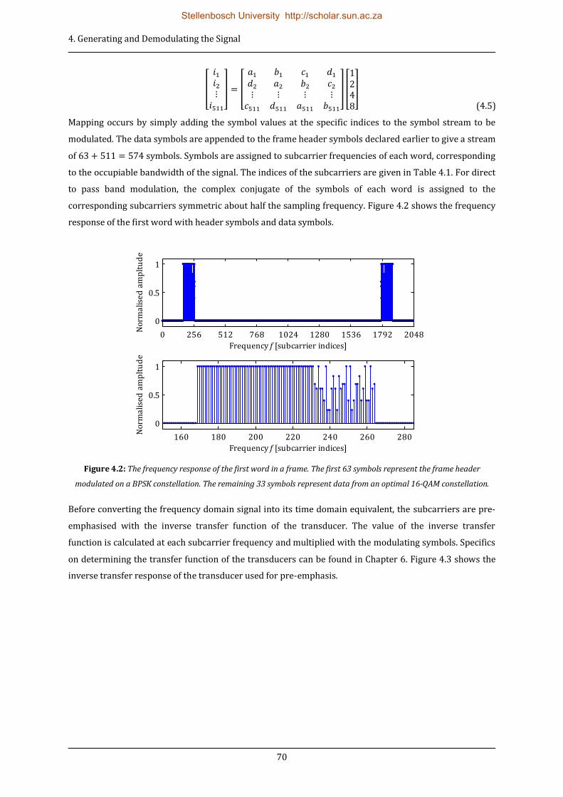
4. Generating and Demodulating the Signal
70
[
] [
] [
]
(4.5)
Mapping occurs by simply adding the symbol values at the specific indices to the symbol stream to be
modulated. The data symbols are appended to the frame header symbols declared earlier to give a stream
of symbols. Symbols are assigned to subcarrier frequencies of each word, corresponding
to the occupiable bandwidth of the signal. The indices of the subcarriers are given in Table 4.1. For direct
to pass band modulation, the complex conjugate of the symbols of each word is assigned to the
corresponding subcarriers symmetric about half the sampling frequency. Figure 4.2 shows the frequency
response of the first word with header symbols and data symbols.
Figure 4.2: The frequency response of the first word in a frame. The first 63 symbols represent the frame header
modulated on a BPSK constellation. The remaining 33 symbols represent data from an optimal 16-QAM constellation.
Before converting the frequency domain signal into its time domain equivalent, the subcarriers are pre-
emphasised with the inverse transfer function of the transducer. The value of the inverse transfer
function is calculated at each subcarrier frequency and multiplied with the modulating symbols. Specifics
on determining the transfer function of the transducers can be found in Chapter 6. Figure 4.3 shows the
inverse transfer response of the transducer used for pre-emphasis.
0 256 512 768 1024 1280 1536 1792 2048
0
0.5
1
No
rma
lised
am
plt
ud
e
Frequency f [subcarrier indices]
160 180 200 220 240 260 280
0
0.5
1
No
rma
lised
am
plt
ud
e
Frequency f [subcarrier indices]
Stellenbosch University http://scholar.sun.ac.za

4. Generating and Demodulating the Signal
71
Figure 4.3: The inverse transfer response of the transducer for the frequency range corresponding to the occupied
bandwidth of the modulated signal.
An IFFT operation is performed on the pre-emphasised frequency domain signal to convert it to the time
domain. The generated word is cyclically extended by prefixing and postfixing 1 ms or 450 samples from
the end and beginning of the word respectively. The cyclic extension serves to absorb the transient
response of the transducer and also the amplitude mask that suppresses out of band radiation. The
amplitude mask takes the form of a raised cosine pulse with the same duration as the extended word,
with 1 ms fade-in and fade-out periods.
Figure 4.4: A cyclically extended OFDM word masked by a raised cosine amplitude mask with 450 samples or 1 ms fade-
in and fade-out to suppress out of band radiation.
Instead of using long periods of cyclic extension to mitigate the intersymbol interference due to multipath
propagation, we append a number of zeros to each word to prolong the intervals between words. The
160 180 200 220 240 260 2800
5
10
15
20
Am
plt
ud
e
Frequency f [subcarrier indices]
160 180 200 220 240 260 280
-90
-45
0
45
90
Ph
ase
an
gle
[d
egr
ee]
Frequency f [subcarrier indices]
0 500 1000 1500 2000 2500 3000
-1
-0.5
0
0.5
1
1.5
No
rma
lised
am
pli
tud
e
Time t [sample indices]
OFDM word
Amplitude mask
Stellenbosch University http://scholar.sun.ac.za

4. Generating and Demodulating the Signal
72
required interval length is dependent on the delay spread and is set to the minimum value that will allow
reliable communication for a particular channel. The construction of a frame is completed by adding a
preamble and postamble to the modulated data words. Figure 4.5 shows a complete frame with 10 ms
intervals between consecutive words.
Figure 4.5: A modulated frame complete with preamble and postamble. The word intervals are set at 10 ms.
The final step in the modulation process is to quantise the signal to 16-bit values. The modulated signal is
generated with double floating point precision. To convert the digital signal into its analogue counterpart,
the signal needs to be in a format compatible with the DAC, i.e. 16-bit integer sample values. The
conversion process involves translating, scaling and rounding each sample to an integer value between 0
and or 65 535. Once converted to 16-bit format the raw signal samples are saved to a binary file
ready for transmission via the transmitter hardware.
4.4 Demodulation Process
As mentioned, the modem design serves as a proof of concept and thus offers only off-line processing of a
received signal. Received signals are recorded in a raw binary format for subsequent processing. The use
of such an unchanging data set allows for experimentation with different modulation techniques on an
equal footing. The fact that results can be graphically represented greatly facilitates the refinement of the
modulation algorithm.
The demodulation process is diagrammatically represented in Figure 4.6.
0 10 20 30 40 50 60 70 80
-1
-0.5
0
0.5
1
No
rma
lised
am
pli
tud
e
Time t [ms]
Stellenbosch University http://scholar.sun.ac.za

4. Generating and Demodulating the Signal
73
Figure 4.6: Diagrammatic representation of the demodulation process.
Demodulation starts off by reading the recorded signal from the file and converting the native 16-bit
integer sample values to double floating point precision values.
The next step involves detection of frames within the signal. This is achieved by cross-correlating the
signal with the preamble and postamble symbols. Impulse-like peaks in the cross-correlations indicate
the positions of the ambles in the signal. Peak detection involves determining points of local maxima
higher than a certain threshold in the envelope of the cross-correlation. The threshold is specified as a
ratio of the RMS value of the cross-correlation. The ratio should be chosen high enough to exclude false
positives, but low enough not to misclassify actual peaks. A threshold of ten times the RMS value is a good
rule of thumb. The peak detection algorithm is fully described in Section 3.3.2. Figure 4.7 and 4.8 shows
the preamble and postamble cross-correlations of one frame from an actual received signal.
Input signal from file
Cross-correlate with ambles
Find peaks by envelope detection
Slice signal into frames
Convert to floating point values
Correct Doppler shift
Extract words and convert to frequency domain
FFT
Determine channel response
Equalize subcarriers and extract symbols
Demap symbols to bit sequences
De-interleave codewords
BCH(511, k) Correct errors by decoding
Output message
Stellenbosch University http://scholar.sun.ac.za
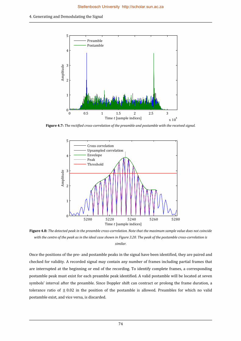
4. Generating and Demodulating the Signal
74
Figure 4.7: The rectified cross-correlation of the preamble and postamble with the received signal.
Figure 4.8: The detected peak in the preamble cross-correlation. Note that the maximum sample value does not coincide
with the centre of the peak as in the ideal case shown in Figure 3.20. The peak of the postamble cross-correlation is
similar.
Once the positions of the pre- and postamble peaks in the signal have been identified, they are paired and
checked for validity. A recorded signal may contain any number of frames including partial frames that
are interrupted at the beginning or end of the recording. To identify complete frames, a corresponding
postamble peak must exist for each preamble peak identified. A valid postamble will be located at seven
symbols’ interval after the preamble. Since Doppler shift can contract or prolong the frame duration, a
tolerance ratio of in the position of the postamble is allowed. Preambles for which no valid
postamble exist, and vice versa, is discarded.
0 0.5 1 1.5 2 2.5 3
x 104
0
1
2
3
4
5
Time t [sample indices]
Am
pli
tud
e
Preamble
Postamble
5200 5220 5240 5260 52800
1
2
3
4
5
Time t [sample indices]
Am
pli
tud
e
Cross correlation
Upsampled correlation
Envelope
Peak
Threshold
Stellenbosch University http://scholar.sun.ac.za

4. Generating and Demodulating the Signal
75
The valid amble pairs are used to slice temporary frames from the signal. 1 ms worth of samples are
included with each slice as overhead before and after the detected preamble and postamble. The
observed interval between the preamble and postamble peaks is used to correct any frequency offset of
the recorded signal. Each temporary slice is resampled at the corresponding rate that will render the
observed interval between the pre- and postamble equal to the supposed interval of seven symbols. To
accurately determine the position of the frame within the slice, a cross-correlation between the preamble
and the first 2 ms of the slice is once more performed. The frame is accurately cropped from the slice to
exclude the cyclic extensions of the preamble and postamble.
Following the successful extraction of the frames from the received signal, we proceed to the channel
estimation process. An FFT is performed on the preamble and postamble of each frame. Following the
least mean squares estimation method discussed in Section 3.3.3, we calculate the channel response as
the element-wise division of the received amble coefficients by the known amble coefficients. We can
write
(4.6)
where denotes channel response coefficients, the received amble coefficients and the known
original amble coefficients. The channel response as determined from the preamble and postamble of an
actual received frame is shown in Figure 4.9.
Figure 4.9: The channel response across the occupied bandwidth calculated from an actual received frame.
The expected time coherence of the underwater channel is fairly short. To compensate for any time
variance we use a weighted average of the preamble and postamble responses to equalise each OFDM
symbol in the frame. The technique can be interpreted as linear interpolation between the frequency
responses in the time domain. We can express the interpolated channel response used to equalise each
OFDM symbol as
38 40 42 44 46 48 50 52 54 56 580
50
100
150
200
Frequency f [kHz]
Am
pli
tud
e
38 40 42 44 46 48 50 52 54 56 58
-180
-90
0
90
180
Ph
ase
an
gle
[de
gree
s]
Frequency f [kHz]
Preamble
Postamble
Stellenbosch University http://scholar.sun.ac.za

4. Generating and Demodulating the Signal
76
(
)
(4.7)
where denotes the channel response vector. Seven is the number of data OFDM symbols per frame plus
one.
With the channel frequency response known we proceed by obtaining the data carrying OFDM symbols
from the frame. An FFT is performed on each OFDM symbol and the coefficients of the occupied
subcarriers are extracted. Equalisation of the extracted symbols is performed by the element-wise
division of the symbols with the channel response corresponding to the particular OFDM symbol. It can
be written as
(4.8)
where represents the equalised symbols, the received symbols and the interpolated channel
response at the particular OFDM symbol. Figure 4.10 shows the 576 equalized symbols of a single frame
on a constellation diagram.
Figure 4.10: 576 equalised symbols from an actual received frame on a constellation diagram. The first 63 symbols of
the first OFDM symbol represents the frame header modulated using BPSK. The rest is 8-QAM symbols. The last two
symbols of OFDM symbol six are zero symbols, representing unoccupied carriers. Symbols are scattered by signal
distortions.
The demapping of the received symbols to bit sequences follows next. The 63 header symbols are
demapped first. For BSK, demapping is performed by evaluating the real part of each symbol; values
larger than zero represents a 1 bit, values smaller than zero represents a 0 bit. The resulting bit stream is
decoded via a ( ) codeword to correct any bit errors. Upon successful decoding, the signal
parameters are extracted from the header.
Once the particular constellation of the data symbols is known, these can be demapped. We use a hard
decision proximity demapping process. The distance from a received symbol to all symbols on the
-1.5 -1 -0.5 0 0.5 1 1.5
-1.5
-1
-0.5
0
0.5
1
1.5
Symbol 1
Symbol 2
Symbol 3
Symbol 4
Symbol 5
Symbol 6
Stellenbosch University http://scholar.sun.ac.za
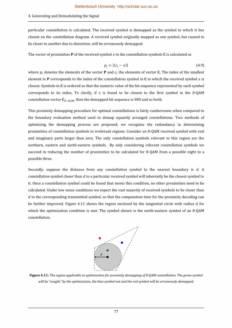
4. Generating and Demodulating the Signal
77
particular constellation is calculated. The received symbol is demapped as the symbol to which it lies
closest on the constellation diagram. A received symbol originally mapped as one symbol, but caused to
lie closer to another due to distortion, will be erroneously demapped.
The vector of proximities of the received symbol to the constellation symbols is calculated as
|( )| (4.9)
where denotes the elements of the vector and the elements of vector . The index of the smallest
element in corresponds to the index of the constellation symbol in to which the received symbol is
closest. Symbols in is ordered so that the numeric value of the bit sequence represented by each symbol
corresponds to its index. To clarify, if is found to be closest to the first symbol in the 8-QAM
constellation vector , then the demapped bit sequence is 000 and so forth.
This proximity demapping procedure for optimal constellations is fairly cumbersome when compared to
the boundary evaluation method used to demap squarely arranged constellations. Two methods of
optimising the demapping process are proposed; we recognise the redundancy in determining
proximities of constellation symbols in irrelevant regions. Consider an 8-QAM received symbol with real
and imaginary parts larger than zero. The only constellation symbols relevant to this region are the
northern, eastern and north-eastern symbols. By only considering relevant constellation symbols we
succeed in reducing the number of proximities to be calculated for 8-QAM from a possible eight to a
possible three.
Secondly, suppose the distance from any constellation symbol to the nearest boundary is . A
constellation symbol closer than to a particular received symbol will inherently be the closest symbol to
it. Once a constellation symbol could be found that meets this condition, no other proximities need to be
calculated. Under low noise conditions we expect the vast majority of received symbols to lie closer than
to the corresponding transmitted symbol, so that the computation time for the proximity decoding can
be further improved. Figure 4.11 shows the region enclosed by the tangential circle with radius for
which the optimisation condition is met. The symbol shown is the north-eastern symbol of an 8-QAM
constellation.
Figure 4.11: The region applicable to optimisation for proximity demapping of 8-QAM constellation. The green symbol
will be “caught” by the optimisation, the blue symbol not and the red symbol will be erroneously demapped.
d
Stellenbosch University http://scholar.sun.ac.za

4. Generating and Demodulating the Signal
78
The same optimisations can be successfully applied to the 16-QAM constellation. It is possible to define
relevant regions different from those set by the real and imaginary axis. However, one should be wary of
introducing more overhead by segmenting the constellation, than it would take to simply calculate one or
two more proximities per region. Further optimisation of the demapping algorithm is possible, but is
regarded as future work.
Once all data symbols have been demapped to bit sequences, the process of error checking and correction
commences. Codewords modulated using 8-QAM and 16-QAM are interleaved prior to the mapping of bit-
sequences to symbols, so that it must be de-interleaved before decoding. De-interspersion is performed
by consecutively cyclically shifting each bit sequence in the opposite direction as the original process.
BPSK and QPSK modulated codewords can be directly decoded as they are not interleaved prior to
mapping. Codewords are decoded via the ( ) code specified by the frame header. If the
decoding of a codeword fails due to excessive bit-errors, the codeword is marked as erroneous and the
data bits are left uncorrected.
The number of bits corresponding to the number of data bytes specified in the frame header is extracted
from the decoded codewords and converted to bytes. Finally the demodulated message together with
message parameters from the frame header is output for further processing by the application layer.
4.5 Summary
This chapter describes the specifications of the physical OFMD signal that the prototype modem transmits
as well as the format of the message data represented by the signal. We also discuss the software
algorithms that manage the signal generation and demodulation, from raw incoming data to an encoded,
interleaved, OFMD modulated and framed signal, and vice versa. In the next chapter we focus on the
hardware design that is tasked with converting the digitised signal samples to acoustic waves that might
propagate through the watery medium to be received and processed by the receiver.
Stellenbosch University http://scholar.sun.ac.za

79
5 TRANSMITTER AND RECEIVER HARDWARE
With a firm grasp on the theoretical workings of OFDM and the specific signal processing requirements
for an underwater communication system, we proceed to identify the hardware requirements for
developing a prototype modem. The specifications of the electronic hardware will mainly be determined
by the particular transducers that are used in the design. For this reason we lead in this chapter with a
discussion on transducers and attempt to characterise the particular devices that are used for the modem.
We also include link budget calculations in order to determine the required transmitter power and
receiver sensitivity to communicate successfully over 1 km. From here we proceed to design electronic
hardware that conforms to these specifications. A synoptic discussion on the transmitter and receiver
explains the workings of each of its composite modules with emphasis on the signal path from the digital
signal to acoustic pressure waves and vice versa. It is noteworthy that all the electronic hardware was
designed and assembled specifically for this prototype modem.
5.1 Transducers
Transducers serve as the interface between the modem and the physical medium. As a projector, this
device is tasked with converting the electrical energy from the power amplifier into acoustic energy that
propagates through the water. As a hydrophone, the transducer will in turn convert the acoustic energy
into an electrical signal for further amplification. Generally, the transducers will be the most expensive,
albeit most restrictive component of any acoustic modem. The main limitation of concern is the frequency
response. The bandwidth and frequency selectivity of a particular transducer will ultimately determine
the achievable performance of the modem. As these devices play such a pivotal role in the design process,
we devote this section to investigate the properties of transducers and how to characterise them.
5.1.1 The Workings of Transducers
Acoustic waves are generated as a result of mechanical vibrations. Transducers function by converting
input electrical energy into mechanical vibrations. They can broadly be divided into two categories
according to the particular technology they employ. Magnetostrictive transducers utilize the properties of
ferromagnetic materials that cause them to undergo a change in dimensions under magnetisation to
create mechanical vibrations. Electrostrictive transducers vibrate as a result of the application of an
alternating electric field that causes a dielectric material to undergo a change in dimensions. Other
mechanisms, such as electrodynamic transducers, explosives, air guns, high voltage discharges across arc
gaps and lasers, are also used as acoustic sources, but have limited application in telemetry systems.
Piezoelectric ceramics are polarized materials that exhibit electrostrictive properties. They are a popular
choice for acoustic underwater transducers, because they are less expensive and provide better
sensitivity and a wider bandwidth than magnetostrictive transducers. The active element consists of a
machined piezoelectric ceramic with electrodes attached to opposite faces of it. When a voltage is applied
Stellenbosch University http://scholar.sun.ac.za

5. Transmitter and Receiver Hardware
80
across the terminals, the polarized molecules of the ceramic align, causing the material to expand or
contract along the direction of the electric field. The ceramic can be cut in different forms to produce
various wave modes. The thickness of the ceramic determines its natural resonant frequency; the thicker
the ceramic, the lower the resonant frequency. The ceramic is cut to a thickness of half the desired
wavelength. Other factors such as the materials used in the construction, the external mechanical and
electrical load conditions and the radiating surface area all influence the behaviour of transducer.
Transducers are constructed by mounting the active element between some backing material and an
impedance matching layer inside a housing. Figure 5.1 shows the construction of a typical piezoelectric
transducer. The backing material has a significant influence on the damping characteristics of the
transducer. A material with a similar acoustic impedance to the ceramic will provide the most efficient
damping, delivering a transducer with a wider bandwidth and a higher sensitivity across its entire
frequency response. The matching layer provides acoustic impedance matching between the ceramic and
the water. For optimal matching the thickness of the matching layer should be a quarter of the desired
wavelength, so that reflected waves within the matching layer remains in phase. The acoustic impedance
of the material is specified between that of the ceramic and water.
Figure 5.1: The construction of a typical piezoelectric transducer.
When used as a hydrophone, the transducer operates according to a similar principle to convert the
mechanical forces exerted by acoustic vibrations into an electric field between the electrodes that can be
detected by the receiver. Not all transducers are designed to perform equally well as projectors and
hydrophones. Projectors are typically driven near their resonant frequency where they provide the
highest acoustic output. Hydrophones generally operate at and below their resonant frequencies over a
much wider frequency band. If a single transducer is to be used for dual purposes, its transmitting and
receiving characteristics should be carefully considered.
5.1.2 The Characteristics of Transducers
The study field of transducers is very large so that we need to limit our discussion to some practical
aspects that are relevant to acoustic communications. The properties that we investigate include the
Bac
kin
g m
ater
ial
Pie
zoel
ectr
ic
cera
mic
Mat
cin
g la
yer
Electrodes
2
4
Hou
sin
g
Stellenbosch University http://scholar.sun.ac.za

5. Transmitter and Receiver Hardware
81
impedance and mechanical quality factor of the equivalent electric circuit, the beam pattern and
directivity index, the transmitting voltage response and open circuit voltage receiving sensitivity.
5.1.2.1 Acoustic Impedance and Sound Intensity Levels
To elucidate the following discussion we digress to define the concepts of acoustic impedance and
intensity before proceeding to the aforementioned properties of transducers. The characteristic acoustic
impedance of water is a material property that is calculated as
(5.1)
with the density of water and the velocity of sound in water.
Acoustic intensity describes the level of acoustic power that is radiated per unit area calculated as
(5.2)
The intensity of a plane harmonic wave can be expressed as a function of the characteristic impedance as
follows
(5.3)
with denoting the pressure variation of the acoustic wave. To compare the intensity levels of sounds we
define a reference intensity for a plane harmonic wave with rms-pressure variations of in water
with density and sound velocity as defined is equation 5.1.
( )
(5.4)
The intensity level of a sound wave is defined relative to the reference intensity so that
(
)
(5.5)
We also define a reference source that will enable us to directly compare acoustic sources with each
other. The reference source is an omni-directional source with as acoustic power output of 1 W taken at
the reference distance of from the acoustic source. Its acoustic intensity is
( )
(5.6)
Its intensity level, relative to the reference intensity of equation 5.4 is
Stellenbosch University http://scholar.sun.ac.za
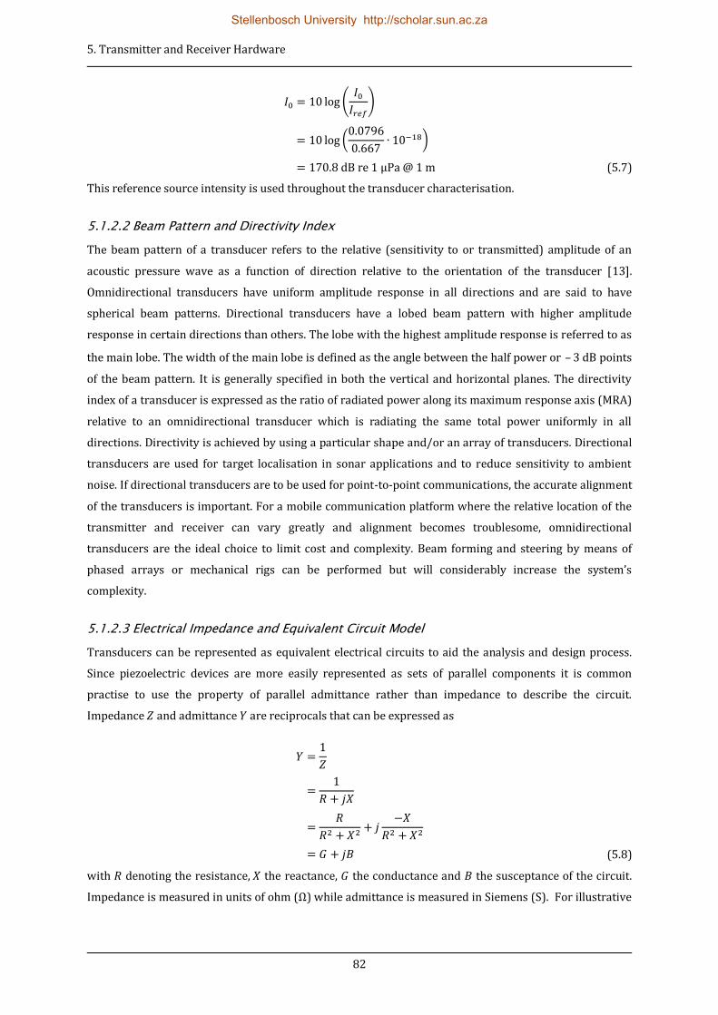
5. Transmitter and Receiver Hardware
82
(
)
(
)
(5.7)
This reference source intensity is used throughout the transducer characterisation.
5.1.2.2 Beam Pattern and Directivity Index
The beam pattern of a transducer refers to the relative (sensitivity to or transmitted) amplitude of an
acoustic pressure wave as a function of direction relative to the orientation of the transducer [13].
Omnidirectional transducers have uniform amplitude response in all directions and are said to have
spherical beam patterns. Directional transducers have a lobed beam pattern with higher amplitude
response in certain directions than others. The lobe with the highest amplitude response is referred to as
the main lobe. The width of the main lobe is defined as the angle between the half power or – points
of the beam pattern. It is generally specified in both the vertical and horizontal planes. The directivity
index of a transducer is expressed as the ratio of radiated power along its maximum response axis (MRA)
relative to an omnidirectional transducer which is radiating the same total power uniformly in all
directions. Directivity is achieved by using a particular shape and/or an array of transducers. Directional
transducers are used for target localisation in sonar applications and to reduce sensitivity to ambient
noise. If directional transducers are to be used for point-to-point communications, the accurate alignment
of the transducers is important. For a mobile communication platform where the relative location of the
transmitter and receiver can vary greatly and alignment becomes troublesome, omnidirectional
transducers are the ideal choice to limit cost and complexity. Beam forming and steering by means of
phased arrays or mechanical rigs can be performed but will considerably increase the system’s
complexity.
5.1.2.3 Electrical Impedance and Equivalent Circuit Model
Transducers can be represented as equivalent electrical circuits to aid the analysis and design process.
Since piezoelectric devices are more easily represented as sets of parallel components it is common
practise to use the property of parallel admittance rather than impedance to describe the circuit.
Impedance and admittance are reciprocals that can be expressed as
(5.8)
with denoting the resistance, the reactance, the conductance and the susceptance of the circuit.
Impedance is measured in units of ohm (Ω) while admittance is measured in Siemens (S). For illustrative
Stellenbosch University http://scholar.sun.ac.za

5. Transmitter and Receiver Hardware
83
purposes the measured conductance and susceptance of an ITC1007 transducer as captured from the
device datasheet is shown in Figure 5.2.
Figure 5.2: Conductance and susceptance of ITC1007 transducer versus frequency.
Figure 5.3 shows the typical equivalent circuit of a piezoelectric transducer.
Figure 5.3: The equivalent circuit model of a piezoelectric transducer.
The components of the equivalent electrical circuit are determined by the frequency dependence of the
conductance and the susceptance of the transducer. Values for the components can be determined from a
conductance-susceptance plot. For illustrative purposes the conductance-susceptance plot of an ITC1007
transducer is shown in Figure 5.4. The points (a, b), where the curve intersects, and (c, d), where the
conductance reaches a maximum, are evaluated to determined the component values.
4 6 8 10 12 14 16 18 20 220
1
2
3
4
5
6
7
8
9
Frequency f [kHz]
Ad
mit
tan
ce Y
= G
+ jB
[m
S]
Conductance G
Susceptance B
0C
C
L
R
Stellenbosch University http://scholar.sun.ac.za
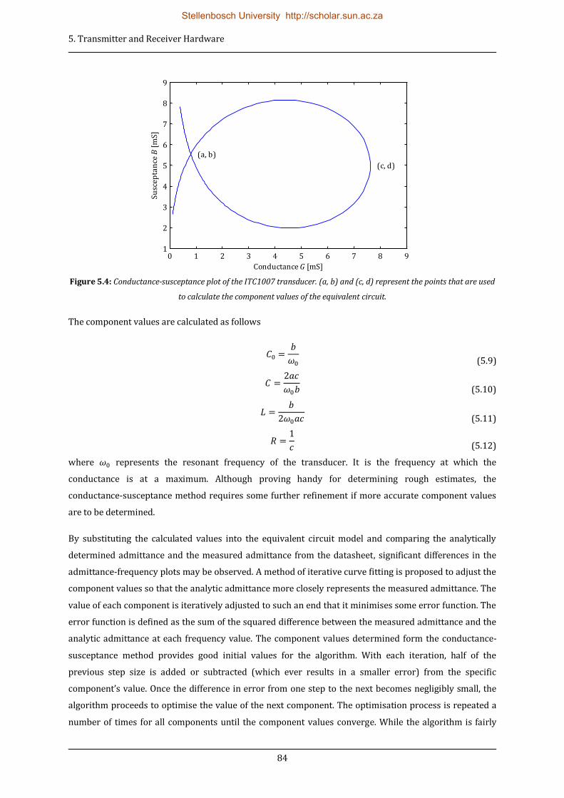
5. Transmitter and Receiver Hardware
84
Figure 5.4: Conductance-susceptance plot of the ITC1007 transducer. (a, b) and (c, d) represent the points that are used
to calculate the component values of the equivalent circuit.
The component values are calculated as follows
(5.9)
(5.10)
(5.11)
(5.12)
where represents the resonant frequency of the transducer. It is the frequency at which the
conductance is at a maximum. Although proving handy for determining rough estimates, the
conductance-susceptance method requires some further refinement if more accurate component values
are to be determined.
By substituting the calculated values into the equivalent circuit model and comparing the analytically
determined admittance and the measured admittance from the datasheet, significant differences in the
admittance-frequency plots may be observed. A method of iterative curve fitting is proposed to adjust the
component values so that the analytic admittance more closely represents the measured admittance. The
value of each component is iteratively adjusted to such an end that it minimises some error function. The
error function is defined as the sum of the squared difference between the measured admittance and the
analytic admittance at each frequency value. The component values determined form the conductance-
susceptance method provides good initial values for the algorithm. With each iteration, half of the
previous step size is added or subtracted (which ever results in a smaller error) from the specific
component’s value. Once the difference in error from one step to the next becomes negligibly small, the
algorithm proceeds to optimise the value of the next component. The optimisation process is repeated a
number of times for all components until the component values converge. While the algorithm is fairly
0 1 2 3 4 5 6 7 8 91
2
3
4
5
6
7
8
9
Conductance G [mS]
Su
scep
tan
ce B
[m
S]
(a, b)
(c, d)
Stellenbosch University http://scholar.sun.ac.za
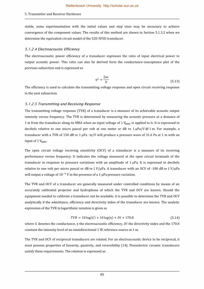
5. Transmitter and Receiver Hardware
85
stable, some experimentation with the initial values and step sizes may be necessary to achieve
convergence of the component values. The results of this method are shown in Section 5.1.3.2 when we
determine the equivalent circuit model of the 520-5PSD transducer.
5.1.2.4 Electroacoustic Efficiency
The electroacoustic power efficiency of a transducer expresses the ratio of input electrical power to
output acoustic power. This ratio can also be derived form the conductance-susceptance plot of the
previous subsection and is expressed as
(5.13)
The efficiency is used to calculate the transmitting voltage response and open circuit receiving response
in the next subsection.
5.1.2.5 Transmitting and Receiving Response
The transmitting voltage response (TVR) of a transducer is a measure of its achievable acoustic output
intensity versus frequency. The TVR is determined by measuring the acoustic pressure at a distance of
1 m from the transducer along its MRA when an input voltage of is applied to it. It is expressed in
decibels relative to one micro pascal per volt at one meter or dB re . For example, a
transducer with a TVR of 150 dB re will produce a pressure wave of 31.6 Pa at 1 m with an
input of .
The open circuit voltage receiving sensitivity (OCV) of a transducer is a measure of its receiving
performance versus frequency. It indicates the voltage measured at the open circuit terminals of the
transducer in response to pressure variations with an amplitude of . It is expressed in decibels
relative to one volt per micro pascal or . A transducer with an OCV of -180
will output a voltage of in the presence of a pressure variation.
The TVR and OCV of a transducer are generally measured under controlled conditions by means of an
accurately calibrated projector and hydrophone of which the TVR and OCV are known. Should the
equipment needed to calibrate a transducer not be available, it is possible to determine the TVR and OCV
analytically if the admittance, efficiency and directivity index of the transducer are known. The analytic
expression of the TVR in logarithmic notation is given as
( ) ( ) (5.14)
where denotes the conductance, the electroacoustic efficiency, the directivity index and the 170.8
constant the intensity level of an omnidirectional 1 W reference source at 1 m.
The TVR and OCV of reciprocal transducers are related. For an electroacoustic device to be reciprocal, it
must possess properties of linearity, passivity, and reversibility [14]. Piezoelectric ceramic transducers
satisfy these requirements. The relation is expressed as
Stellenbosch University http://scholar.sun.ac.za

5. Transmitter and Receiver Hardware
86
| | (5.15)
where denotes the impedance of the transducer and the reciprocity parameter. For spherical
propagation, is given as
(5.16)
where is the reference distance at which the TVR is specified, i.e. 1 m and denotes frequency. In
logarithmic notation, with the OCV specified with reference to pressure in , we can take as
( ) (5.17)
with the frequency in kHz [13].
For illustrative purposes the TVR and OCV of an ITC 1007 transducer as captured from the device
datasheet is shown in Figure 5.5 and 5.6.
Figure 5.5: The measured TVR from the datasheet of an ITC 1007 transducer.
4 6 8 10 12 14 16 18 20 22125
130
135
140
145
150
Frequency f [kHz]
TV
R [
dB
re
1
Pa/
V @
1m
]
Stellenbosch University http://scholar.sun.ac.za

5. Transmitter and Receiver Hardware
87
Figure 5.6: The measured OCR from the datasheet of an ITC1007 transducer.
Transducers suitable for use in communication systems should have a transmitting and/or a receiving
response that is as flat as possible over the frequency band of interest. The half power or
bandwidth should be wide enough to allow for sufficient data throughput. The centre frequency should be
as low as possible to limit frequency dependant absorption. The choice of bandwidth and centre
frequency primarily rests on whether the data throughput or operational range takes priority in the
design specifications of the modem. If a single transducer is to be used as both a projector and
hydrophone, the effective bandwidth of the device should be considered as that frequency range between
the points of the product of the TVR and OCV.
5.1.3 Characterisation of Furuno 520-5PSD Transducers
The devices used for this prototype modem is the 520-5PSD transducer manufactured by Furuno. These
were available from a previous project and to avoid the purchase of more expensive models it was
thought fit to include it in the initial design.
The 520-5PSD is designed for fish and depth finder applications. Detailed specifications of these devices,
i.e. the beam pattern, directivity index, impedance, OCV and TVR are not available. Table 5.1 shows the
extent of the specifications that can be found on the internet [15].
Parameter
Resonant frequencies 50 kHz and 200 kHz
Beam width at resonance 46° and 10° respectively
Output power (1% duty cycle) 600 W
Housing and mounting type Plastic though-hull
Connection 8 m cable with 10-pin connector
Table 5.1: The limited specifications of Furuno 520-5PSD transducers.
4 6 8 10 12 14 16 18 20 22-205
-200
-195
-190
-185
-180
Frequency f [kHz]
OC
R [
dB
re
1V
/P
a]
Stellenbosch University http://scholar.sun.ac.za
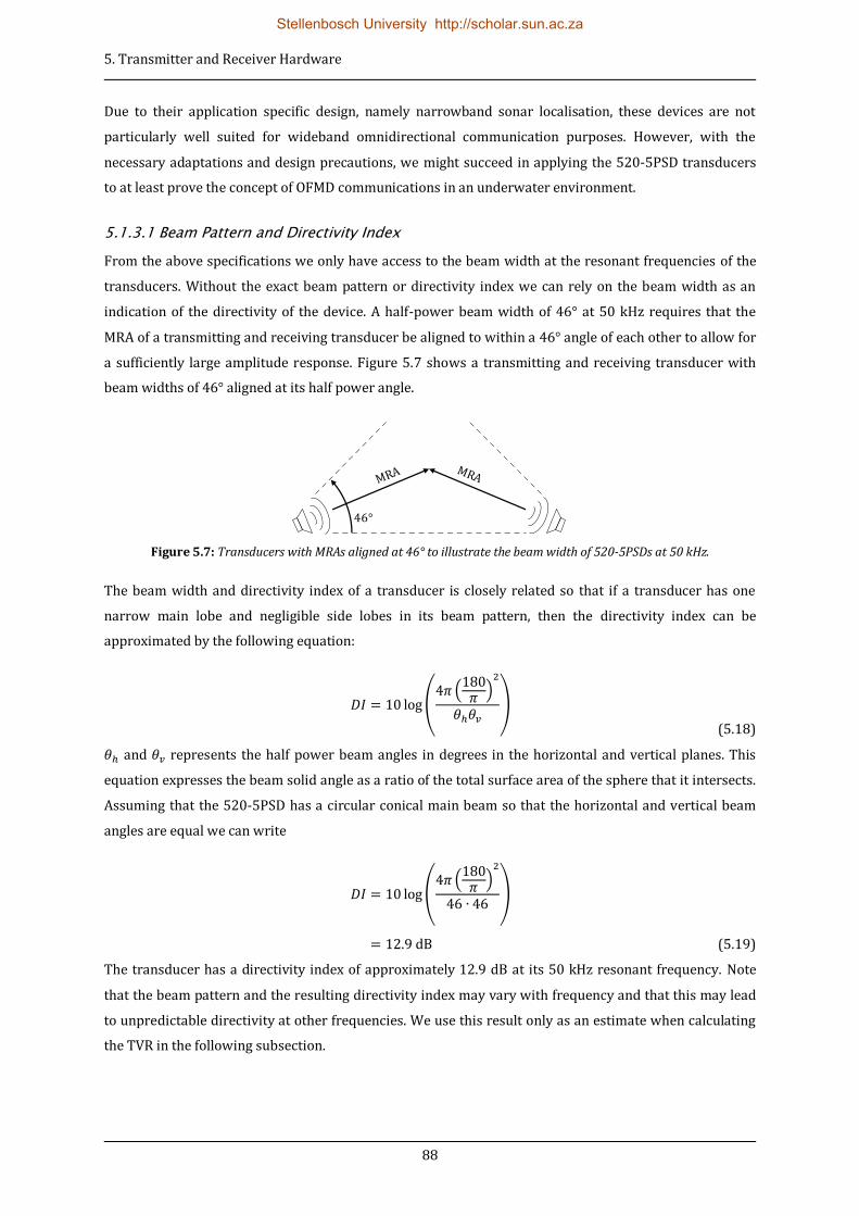
5. Transmitter and Receiver Hardware
88
Due to their application specific design, namely narrowband sonar localisation, these devices are not
particularly well suited for wideband omnidirectional communication purposes. However, with the
necessary adaptations and design precautions, we might succeed in applying the 520-5PSD transducers
to at least prove the concept of OFMD communications in an underwater environment.
5.1.3.1 Beam Pattern and Directivity Index
From the above specifications we only have access to the beam width at the resonant frequencies of the
transducers. Without the exact beam pattern or directivity index we can rely on the beam width as an
indication of the directivity of the device. A half-power beam width of 46° at 50 kHz requires that the
MRA of a transmitting and receiving transducer be aligned to within a 46° angle of each other to allow for
a sufficiently large amplitude response. Figure 5.7 shows a transmitting and receiving transducer with
beam widths of 46° aligned at its half power angle.
Figure 5.7: Transducers with MRAs aligned at 46° to illustrate the beam width of 520-5PSDs at 50 kHz.
The beam width and directivity index of a transducer is closely related so that if a transducer has one
narrow main lobe and negligible side lobes in its beam pattern, then the directivity index can be
approximated by the following equation:
( (
)
)
(5.18)
and represents the half power beam angles in degrees in the horizontal and vertical planes. This
equation expresses the beam solid angle as a ratio of the total surface area of the sphere that it intersects.
Assuming that the 520-5PSD has a circular conical main beam so that the horizontal and vertical beam
angles are equal we can write
( (
)
)
(5.19)
The transducer has a directivity index of approximately 12.9 dB at its 50 kHz resonant frequency. Note
that the beam pattern and the resulting directivity index may vary with frequency and that this may lead
to unpredictable directivity at other frequencies. We use this result only as an estimate when calculating
the TVR in the following subsection.
MRA MRA
46°
Stellenbosch University http://scholar.sun.ac.za

5. Transmitter and Receiver Hardware
89
5.1.3.2 Measuring the Electrical Impedance and Fitting the Equivalent Circuit Model
Nothing, other than the resonant frequencies, is known about the frequency response of the 520-5PSD
transducers. In an attempt to predict the TVR and OCR of these devices, we set out to characterise it by
determining the impedance and fitting an equivalent electrical circuit model to it, following the methods
described in the previous subsection.
Firstly, the admittance of the transducer is measured with a spectrum analyser. The wet and dry
admittance of the transducer differ, so that it must be submerged when analysing it. The voltage across a
series resistor is used to measure the current through the transducer, together with the voltage across the
device’s terminals. Voltage, current and phase measurements are recorded in increments of 250 Hz
across the frequency band from 35 kHz to 65 kHz. The admittance is calculated following the inverse of
Ohm’s law. The measured admittance is shown in Figure 5.8.
Figure 5.8: The submerged admittance of a 520-5PSD transducer measured with a spectrum analyser.
Once the admittance of the transducer is known, a conductance-susceptance plot can be drawn. From this
plot, component values for the equivalent circuit model can be derived. The conductance-susceptance
plot of the measured admittance is shown in Figure 5.9.
35 40 45 50 55 60 65-2
-1
0
1
2
3
4
5
Frequency f [kHz]
Ad
mit
tan
ce Y
= G
+ jB
[m
S]
Conductance G
Susceptance B
Stellenbosch University http://scholar.sun.ac.za

5. Transmitter and Receiver Hardware
90
Figure 5.9: The conductance-susceptance plot of a 520-5PSD transducer.
As can be seen from the plot, the curve never intersects at the point (a, b). Given that the conductance-
susceptance method provides only a rough estimate of component values, it should be safe to estimate
the intersection point at ( ). With frequency intervals as large as 250 Hz, the curve
shows discontinuities at the point of maximum conductance. We choose the point (
) measured at 49.75 kHz as the point of maximum conductance. To obtain the component values, we
substitute these points into the equations of Section 5.1.2.3.
(5.20)
(5.21)
(5.22)
(5.23)
0 1 2 3 4 5-2
-1
0
1
2
3
Conductance G [mS]
Su
scep
tan
ce B
[m
S]
(a, b)(c, d)
Stellenbosch University http://scholar.sun.ac.za

5. Transmitter and Receiver Hardware
91
Figure 5.10 compares the admittance calculated from the equivalent circuit using the values obtained
above with the admittance as measured by the spectrum analyser. The resonant frequency is accurate,
but the bandwidth is slightly wider than that of the measured results.
Figure 5.10: The admittance of a 520-5PSD transducer as measured with the spectrum analyser and as determined
from the equivalent circuit model with component values derived by the conductance-susceptance method.
The values obtained from the conductance-susceptance method are used as the initial values in the
iterative curve fitting algorithm. The algorithm iteratively adjusts the component values until the
resulting conductance and susceptance curves approach the measured values with ever increasing
accuracy. This is achieved by minimising an error function that is calculated as the sum of the admittance
errors at all frequencies. The algorithm is described in Section 5.1.2.3. The optimized component values
as determined by iterative curve fitting are as follows:
(5.24)
Figure 5.11 compares the admittance plots of the measured results, the initial component values and the
optimised component values. The optimized component values represent the measured admittance very
closely and we can assume that the equivalent circuit model for the 520-5PSD transducer is highly
accurate over the frequency band of interest.
35 40 45 50 55 60 65-2
-1
0
1
2
3
4
5
Frequency f [kHz]
Ad
mit
tan
ce Y
= G
+ jB
[m
S]
Measured G
Measured B
Derived G
Derived B
Stellenbosch University http://scholar.sun.ac.za

5. Transmitter and Receiver Hardware
92
Figure 5.11: The admittance of a 520-5PSD transducer determined from the optimised values of the equivalent circuit
model shown in comparison with the measured results and the initial values from the conductance-susceptance method.
5.1.3.3 Determining the Electroacoustic Efficiency
In order to accurately determine the electroacoustic efficiency of the 520-5PSD transducer we use the
newly calculated admittance to plot a conductance-susceptance curve, shown in Figure 5.12, from which
the intersection and maximum conductance points can be found. The intersection point is at (
). The point of maximum conductance point is at ( ). The
resulting electroacoustic efficiency is
( )
(5.25)
35 40 45 50 55 60 65-2
-1
0
1
2
3
4
5
Frequency f [kHz]
Ad
mit
tan
ce Y
= G
+ jB
[m
S]
Measured G
Measured B
Derived G
Derived B
Optimised G
Optimised B
Stellenbosch University http://scholar.sun.ac.za
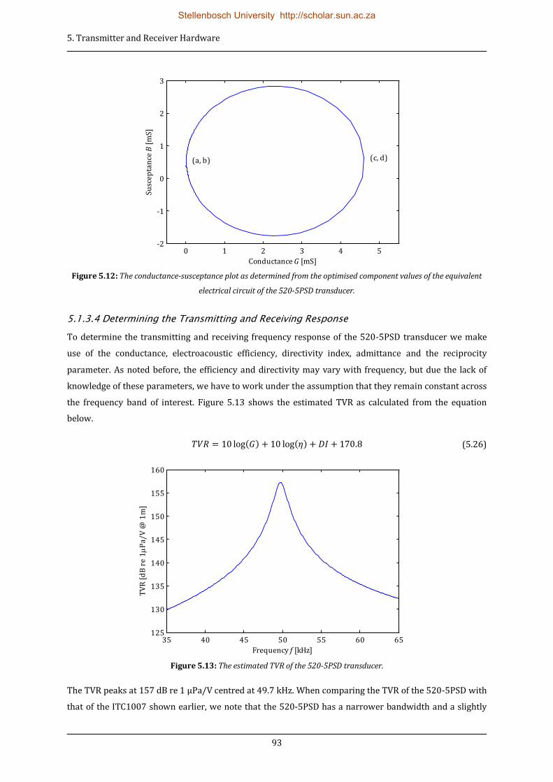
5. Transmitter and Receiver Hardware
93
Figure 5.12: The conductance-susceptance plot as determined from the optimised component values of the equivalent
electrical circuit of the 520-5PSD transducer.
5.1.3.4 Determining the Transmitting and Receiving Response
To determine the transmitting and receiving frequency response of the 520-5PSD transducer we make
use of the conductance, electroacoustic efficiency, directivity index, admittance and the reciprocity
parameter. As noted before, the efficiency and directivity may vary with frequency, but due the lack of
knowledge of these parameters, we have to work under the assumption that they remain constant across
the frequency band of interest. Figure 5.13 shows the estimated TVR as calculated from the equation
below.
( ) ( ) (5.26)
Figure 5.13: The estimated TVR of the 520-5PSD transducer.
The TVR peaks at 157 centred at 49.7 kHz. When comparing the TVR of the 520-5PSD with
that of the ITC1007 shown earlier, we note that the 520-5PSD has a narrower bandwidth and a slightly
0 1 2 3 4 5-2
-1
0
1
2
3
Conductance G [mS]
Su
scep
tan
ce B
[m
S]
(a, b) (c, d)
35 40 45 50 55 60 65125
130
135
140
145
150
155
160
Frequency f [kHz]
TV
R [
dB
re
1
Pa/
V @
1m
]
Stellenbosch University http://scholar.sun.ac.za
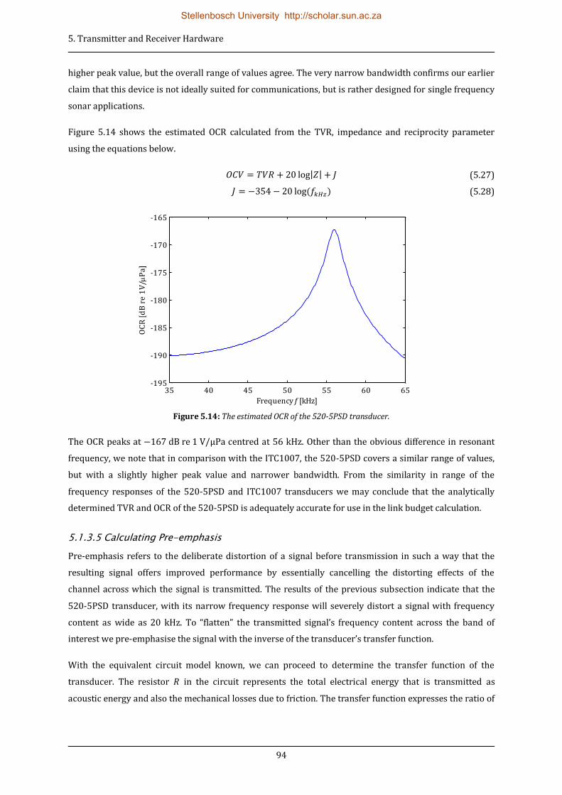
5. Transmitter and Receiver Hardware
94
higher peak value, but the overall range of values agree. The very narrow bandwidth confirms our earlier
claim that this device is not ideally suited for communications, but is rather designed for single frequency
sonar applications.
Figure 5.14 shows the estimated OCR calculated from the TVR, impedance and reciprocity parameter
using the equations below.
| | (5.27)
( ) (5.28)
Figure 5.14: The estimated OCR of the 520-5PSD transducer.
The OCR peaks at centred at 56 kHz. Other than the obvious difference in resonant
frequency, we note that in comparison with the ITC1007, the 520-5PSD covers a similar range of values,
but with a slightly higher peak value and narrower bandwidth. From the similarity in range of the
frequency responses of the 520-5PSD and ITC1007 transducers we may conclude that the analytically
determined TVR and OCR of the 520-5PSD is adequately accurate for use in the link budget calculation.
5.1.3.5 Calculating Pre-emphasis
Pre-emphasis refers to the deliberate distortion of a signal before transmission in such a way that the
resulting signal offers improved performance by essentially cancelling the distorting effects of the
channel across which the signal is transmitted. The results of the previous subsection indicate that the
520-5PSD transducer, with its narrow frequency response will severely distort a signal with frequency
content as wide as 2 kHz. To “flatten” the transmitted signal’s frequency content across the band of
interest we pre-emphasise the signal with the inverse of the transducer’s transfer function.
With the equivalent circuit model known, we can proceed to determine the transfer function of the
transducer. The resistor in the circuit represents the total electrical energy that is transmitted as
acoustic energy and also the mechanical losses due to friction. The transfer function expresses the ratio of
35 40 45 50 55 60 65-195
-190
-185
-180
-175
-170
-165
Frequency f [kHz]
OC
R [
dB
re
1V
/P
a]
Stellenbosch University http://scholar.sun.ac.za
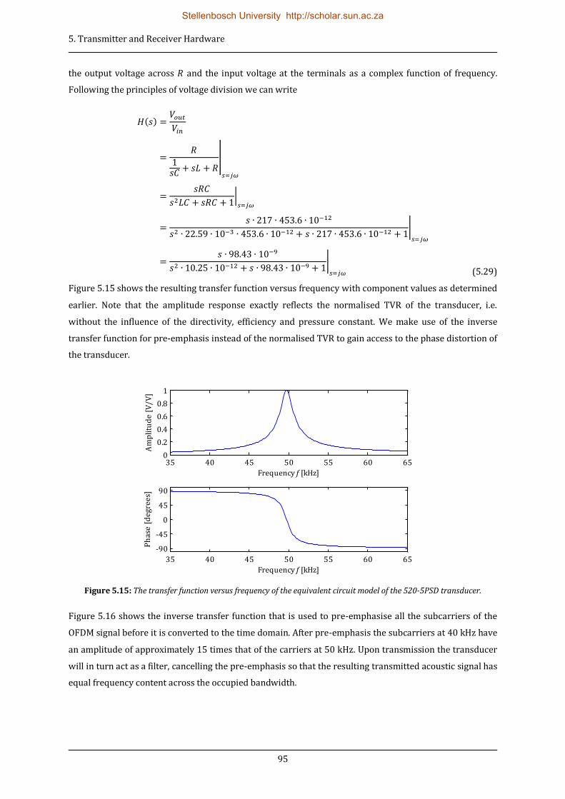
5. Transmitter and Receiver Hardware
95
the output voltage across and the input voltage at the terminals as a complex function of frequency.
Following the principles of voltage division we can write
( )
|
|
|
|
(5.29)
Figure 5.15 shows the resulting transfer function versus frequency with component values as determined
earlier. Note that the amplitude response exactly reflects the normalised TVR of the transducer, i.e.
without the influence of the directivity, efficiency and pressure constant. We make use of the inverse
transfer function for pre-emphasis instead of the normalised TVR to gain access to the phase distortion of
the transducer.
Figure 5.15: The transfer function versus frequency of the equivalent circuit model of the 520-5PSD transducer.
Figure 5.16 shows the inverse transfer function that is used to pre-emphasise all the subcarriers of the
OFDM signal before it is converted to the time domain. After pre-emphasis the subcarriers at 40 kHz have
an amplitude of approximately 15 times that of the carriers at 50 kHz. Upon transmission the transducer
will in turn act as a filter, cancelling the pre-emphasis so that the resulting transmitted acoustic signal has
equal frequency content across the occupied bandwidth.
35 40 45 50 55 60 650
0.2
0.4
0.6
0.8
1
Frequency f [kHz]
Am
pli
tud
e [
V/
V]
35 40 45 50 55 60 65
-90
-45
0
45
90
Frequency f [kHz]
Ph
ase
[d
egr
ees]
Stellenbosch University http://scholar.sun.ac.za

5. Transmitter and Receiver Hardware
96
Figure 5.16: The inverse transfer function used in the pre-emphasis of the signal before transmission.
The receiving response of the transducer is not included in the pre-emphasis. With the transmitted signal
having a flat frequency response and assuming that any ambient noise present in the channel is white, the
received signal will have a constant SNR across all subcarriers in the occupied frequency band. This
ensures that no sub-band of frequencies suffers from a lower SNR than others. It simplifies the calculation
of the SNR to be used in the adaptive modulation scheme and also ensures that symbol errors are
uniformly spread across the entire bandwidth and not concentrated in a frequency band. The distortion
resulting from the uneven OCR of the receiving transducer is compensated for by the channel equalisation
process. The influence of the uneven receiving response is notably visible in the results of the channel
estimation, shown in the next chapter.
5.2 Link Budget
In order to establish a reliable wireless communication link over some distance, factors such as the
required transmitter power, transducer directivity gains, anticipated channel losses and receiver
sensitivity should be carefully considered. In telecommunications a link budget accounts for all the gains
and losses that a signal might encounter as it propagates from the transmitter, through the physical
medium, to the receiver. A typical link budget equation is composed as follows
( ) ( ) ( ) ( ) (5.30)
5.2.1 Theory of Acoustic Link Budget
For an acoustic link budget we make use of sound intensity levels as a measure of the acoustic power
radiated per unit area. The intensity level of an acoustic source relative to the intensity of a plane wave
with RMS pressure of is defined as
( ) ( ) (5.31)
35 40 45 50 55 60 650
5
10
15
20
25
Frequency f [kHz]
Am
pli
tud
e [
V/
V]
35 40 45 50 55 60 65
-90
-45
0
45
90
Frequency f [kHz]
Ph
ase
[d
egr
ees]
Stellenbosch University http://scholar.sun.ac.za

5. Transmitter and Receiver Hardware
97
with the source level, the input electrical power, the electroacoustic efficiency, the directivity
index and 170.8 the intensity of a spherical 1 W source at 1 m relative to the intensity of a plane wave
with RMS pressure of . The unit is . Consider that the electrical input power can be
written as
(5.32)
with the input voltage and the resistance. is the reciprocal of the conductance G so that
(5.33)
By substituting this into the source level equation we obtain
( ) ( ) ( ) (5.34)
Upon closer inspection we realise that this represents the TVR of a transducer so that we may express the
source level as
( ) (5.35)
The acoustic intensity level at some distance away from the source is expressed as
(5.36)
with representing the transmission loss due to spreading and attenuation. From Chapter 2 we have
that spherical spreading diminishes the intensity of an acoustic wave proportional to the square of the
distance covered. Attenuation due to absorption can vary significantly with frequency, pressure,
temperature, salinity and acidity. The expected attenuation in dB/m can be determined from equation
2.23 for a given set of conditions. The combined transmission loss is expressed as
( ) (5.37)
with the distance from the source in m and the attenuation constant in dB/m.
The anticipated open circuit voltage of a receiving transducer with known sensitivity can be calculated as
follows
( ) (5.38)
We can combine equations 5.35, 5.36 and 5.38 to write
( ) ( ) (5.39)
By expressing the acoustic link budget in terms of the TVR and OCR of a transducer we can directly
determine the anticipated voltage levels at the transmitter and receiver. The TVR and OCR already
include gain and loss factors such as the directivity index and non-ideal electroacoustic efficiency that
would normally be treated separately in a conventional link budget.
Stellenbosch University http://scholar.sun.ac.za

5. Transmitter and Receiver Hardware
98
5.2.2 Link Budget Over 1 km
The objectives of this project stipulate that the prototype modem should be able to communicate
successfully across a distance of 1 km. To determine the required gain Figures of the transmitter and
receiver we compose a link budget that is representative of the acoustic communication link across 1 km.
The transducer’s TVR and OCR vary significantly across the occupied bandwidth of the OFDM signal. For
this reason we choose to calculate the link budget by adding and subtracting the frequency response of
each term of equation 5.39 across the entire occupied bandwidth. Figure 5.17 shows the frequency
responses of the terms as they occur in equation 5.39.
Figure 5.17: The frequency responses of the terms in the link budget. The top four responses representing the input
voltage, TVR, transmission losses and OCR are summed to give the response of the output voltage in the bottom plot.
The first plot represents the input voltage from the power amplifier that drives the transducer. This
signal is pre-emphasised in order to counterbalance the response of the TVR of the transducer. The plot
35 40 45 50 55 60 65-20
-10
0
10
Vin
[d
B]
35 40 45 50 55 60 65130
140
150
160
TV
R [
dB
re
1
Pa/
V]
35 40 45 50 55 60 65-190
-180
-170
-160
OC
R [
dB
re
1 V
/P
a]
35 40 45 50 55 60 65-75
-70
-65
TL
[d
B]
35 40 45 50 55 60 65-120
-110
-100
-90
Vo
ut [
dB
]
Frequency f [kHz]
Stellenbosch University http://scholar.sun.ac.za

5. Transmitter and Receiver Hardware
99
was generated from the frequency response of a typical OFDM symbol that is amplified to the maximum
output levels of the power amplifier, i.e. . The details of the power amplifier are discussed in
Section 5.3.4.
The TVR of the transducer in the second plot is from the previous section. By adding the input voltage and
TVR a flat response of 143.7 dB is obtained.
The transmission loss plot, indicated as a negative gain on the figure, shows the combined effect of
spherical spreading and attenuation due to absorption. With spherical spreading over 1 km the
anticipated loss is
( )
(5.40)
The attenuation due to absorption is calculated from the equation in [6] for water with a salinity of
35 ppm, pH of 8 and a temperature of at a depth of 1 m. The resulting attenuation loss increases
from 7.2 dB at 40 kHz to 14.6 dB at 60 kHz.
The OCR of the transducer in the fourth plot is from the previous section.
By summing all of the above mentioned responses, we obtain the response of the open circuit voltage
output of the receiving transducer shown in the last plot. The time domain equivalent of the received
voltage response shows a peak amplitude of . Prior to the analogue-to-digital conversion of the
received signal it must be amplified to levels corresponding to the input range of the digital-to-analogue
converter, i.e. or . The required gain of the receiver is calculated as
( )
(5.41)
The details of the receiver design are discussed in Section 5.4.
5.3 Electronic Hardware of the Transmitter
It is the task of the transmitter to take the digital modulated signal as input and translating it into acoustic
pressure waves that propagate through the physical medium. Figure 5.18 depicts the modular hardware
chain and the steps involved in converting the signal from its digital format into an analogue equivalent.
Figure 5.19 shows the modular layout of the electronics that make up the transmitter. In the following
subsections we discuss each of the modules and also consider the interfaces between them.
Stellenbosch University http://scholar.sun.ac.za
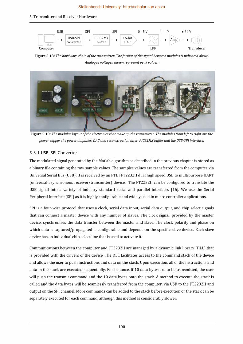
5. Transmitter and Receiver Hardware
100
Figure 5.18: The hardware chain of the transmitter. The format of the signal between modules is indicated above.
Analogue voltages shown represent peak values.
Figure 5.19: The modular layout of the electronics that make up the transmitter. The modules from left to right are the
power supply, the power amplifier, DAC and reconstruction filter, PIC32MX buffer and the USB-SPI interface.
5.3.1 USB-SPI Converter
The modulated signal generated by the Matlab algorithm as described in the previous chapter is stored as
a binary file containing the raw sample values. The samples values are transferred from the computer via
Universal Serial Bus (USB). It is received by an FTDI FT2232H dual high speed USB to multipurpose UART
(universal asynchronous receiver/transmitter) device. The FT2232H can be configured to translate the
USB signal into a variety of industry standard serial and parallel interfaces [16]. We use the Serial
Peripheral Interface (SPI) as it is highly configurable and widely used in micro controller applications.
SPI is a four-wire protocol that uses a clock, serial data input, serial data output, and chip select signals
that can connect a master device with any number of slaves. The clock signal, provided by the master
device, synchronises the data transfer between the master and slave. The clock polarity and phase on
which data is captured/propagated is configurable and depends on the specific slave device. Each slave
device has an individual chip select line that is used to activate it.
Communications between the computer and FT2232H are managed by a dynamic link library (DLL) that
is provided with the drivers of the device. The DLL facilitates access to the command stack of the device
and allows the user to push instructions and data on the stack. Upon execution, all of the instructions and
data in the stack are executed sequentially. For instance, if 10 data bytes are to be transmitted, the user
will push the transmit command and the 10 data bytes onto the stack. A method to execute the stack is
called and the data bytes will be seamlessly transferred from the computer, via USB to the FT2232H and
output on the SPI channel. More commands can be added to the stack before execution or the stack can be
separately executed for each command, although this method is considerably slower.
USB-SPI converter
PIC32MX buffer
SPI
16-bit DAC
SPI 0 - 5 V ± 60 V
Amp
Transducer Computer
USB 0 - 5 V
LPF
Stellenbosch University http://scholar.sun.ac.za

5. Transmitter and Receiver Hardware
101
The stack has a capacity of 64 kB. This limits the number of 16-bit samples that can be transferred with
each execution of the stack to 32 k. The SPI link of the FT2232H operates at a clock speed of 30 Mbps. To
transfer a block of 32 k samples from the computer to the PIC32MX buffer thus takes approximately
17 ms. The buffer dispatches samples to the DAC at a rate of 450 kHz. At this rate the 32 k samples will
last 71 ms. This means that the FT2232H has to transfer a block of 32 k samples from the computer to the
PIC32MX buffer once every 71 ms to maintain the continuity of the signal.
5.3.2 PIC32MX Buffer
The FT2232H does not provide a means of generating a 450 kHz timing signal that can be used to control
the conversion rate of a DAC. For this reason it is necessary to temporarily store the sample values in a
buffer as the 32 k sample blocks are received from the computer. A Microchip PIC32MX795F52H micro
controller, operating at a clock speed of 80 MHz and with 128 kB SRAM [17], provides ample performance
for this purpose. It has two SPI channels that can be individually configured. The first is setup as a slave to
be controlled by the FT2232H. The second acts as a master device to control the DAC.
The buffering algorithm utilises a dual interchanging queue structure. Two 64 kB queues, holding 32 k
samples each, are alternately filled with samples from the FT2232H. Once a queue is full, samples from it
are transmitted to the DAC via the second SPI channel. The alternate queue simultaneously receives
samples from the FT2232H via the first SPI channel. Once all of the samples from the first queue have
been transmitted, transmission switches to the alternate queue and the FT2232H is signalled to dispatch
another 32 k sample block to again fill the first queue. Synchronisation between the PIC32MX and the
FT2232H is achieved via the chip select line. Indicator flags are used to determine the state of each queue,
i.e. which queue is transmitted from, which queue is to be filled and which queues are empty/full. This
alternation between the queues continues until no new samples are received from the FT2232H and both
queues have been emptied.
The PIC32MX is configured to generate timed interrupts at 450 kHz. With each interrupt a new sample
value is to be output to the DAC. The interrupt checks the queue status flags and if samples are available
in the buffer it transmits the next sample from the corresponding queue. The status flags are updated
accordingly if the last sample in a queue has been transmitted. If no samples are available, then the device
simply outputs a zero value.
5.3.3 Digital-to-analogue Converter and Reconstruction Filter
A DAC8830 digital-to-analogue converter (DAC) from Texas Instruments is used to convert the digital
signal samples into an analogue voltage signal. The DAC8830 is a single, 16-bit, serial input, voltage-
output DAC operating from a single 3 V to 5 V power supply. These converters provide excellent linearity
of 1 least significant bit (LSB) integral nonlinearity (INL), low glitch, low noise and a fast settling time of
to ½ LSB of the full-scale output over the temperature range of to [18]. It also offers a
standard high-speed 3 V to 5 V SPI interface accepting clock speeds of up to 50 MHz [18].
Stellenbosch University http://scholar.sun.ac.za

5. Transmitter and Receiver Hardware
102
Samples from the PIC32MX buffer are dispatched to the DAC8830 via the SPI channel at a transfer rate of
40 Mbps. The PIC32MX buffer acts as the master device that supplies the clock signal used to synchronise
the data transfer. Once a sample value has been clocked into the DAC, the analogue output voltage is
enabled upon a rising edge on the device’s chip select line. A 5 V analogue reference source provides an
output swing of centred at 2.5 V. An output-compare timer of the PIC32MX controls the
conversion rate by outputting pulses at intervals of 2.222 µs or 450 kHz on the chip select line of the
DAC8830. This timer also triggers the interrupts mentioned in the previous subsection.
An active first-order low-pass filter acts as a buffer between the DAC and the power amplifier. Designed
with an RC-time constant of , this filter acts a reconstruction filter that suppresses the
overshoot and ringing during the settling time of the DAC. The sample intervals of allows
the output of the filter to asymptotically approach the final settling value to within 98 %.
5.3.4 Power Amplifier
The final stage of amplification that drives the transducers is provided by a set of bridged LM3886 power
amplifiers. The high impedance of the transducer necessitates a bridged configuration that provides a
larger output voltage swing to increase the transmitted power. The LM3886 is a high-performance audio
amplifier capable of delivering 68 W of continuous power to a 4 Ω load and 38W into 8Ω with . % total
harmonic distortion plus noise (THD+N) from with a supply voltage of [19].
These devices are designed for optimal performance across the audio frequency spectrum. However, with
a quoted gain-bandwidth-product (GBWP) of 8 MHz (typical) and slew rate of 19 V/µs (typical) it should
still provide sufficient performance across the frequency band of interest at .
A power supply of is used to power the LM3886 amplifiers allowing an output voltage swing
of approximately with minimal distortion. In a bridged configuration with an inverting
and non-inverting device in series this translates to a swing of or . With an input signal
from the LPF of , a voltage gain of
(5.42)
is required to cover the output range of the amplifier. The external component values are designed so that
the inverting and non-inverting amplifiers have equal gains of 12. The required GBWP of an amplifier is
typically specified as the product of five times the maximum bandwidth of the input signal and the closed
loop gain. With a maximum input frequency of 60 kHz and a gain of 12, the required GBWP is calculated
as
Stellenbosch University http://scholar.sun.ac.za
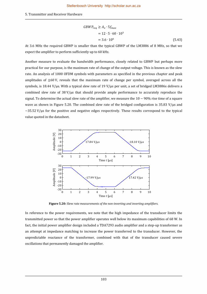
5. Transmitter and Receiver Hardware
103
(5.43)
At 3.6 MHz the required GBWP is smaller than the typical GBWP of the LM3886 of 8 MHz, so that we
expect the amplifier to perform sufficiently up to 60 kHz.
Another measure to evaluate the bandwidth performance, closely related to GBWP but perhaps more
practical for our purpose, is the maximum rate of change of the output voltage. This is known as the slew
rate. An analysis of 1000 OFDM symbols with parameters as specified in the previous chapter and peak
amplitudes of , reveals that the maximum rate of change per symbol, averaged across all the
symbols, is 18.44 V/µs. With a typical slew rate of 19 V/µs per unit, a set of bridged LM3886s delivers a
combined slew rate of 38 V/µs that should provide ample performance to accurately reproduce the
signal. To determine the actual slew rate of the amplifier, we measure the rise time of a square
wave as shown in Figure 5.20. The combined slew rate of the bridged configuration is 35.83 V/µs and
for the positive and negative edges respectively. These results correspond to the typical
value quoted in the datasheet.
Figure 5.20: Slew rate measurements of the non-inverting and inverting amplifiers.
In reference to the power requirements, we note that the high impedance of the transducer limits the
transmitted power so that the power amplifier operates well below its maximum capabilities of 68 W. In
fact, the initial power amplifier design included a TDA7293 audio amplifier and a step-up transformer as
an attempt at impedance matching to increase the power transferred to the transducer. However, the
unpredictable reactance of the transformer, combined with that of the transducer caused severe
oscillations that permanently damaged the amplifier.
0 1 2 3 4 5 6 7 8 9 10-30
-20
-10
0
10
20
30
Time t [s]
Am
pli
tud
e [
V]
17.84 V/s -18.10 V/s
0 1 2 3 4 5 6 7 8 9 10-30
-20
-10
0
10
20
30
Time t [s]
Am
pli
tud
e [
V]
-17.99 V/s 17.42 V/s
Stellenbosch University http://scholar.sun.ac.za

5. Transmitter and Receiver Hardware
104
5.4 Electronic Hardware of the Receiver
In broad outline, the function of the receiver can be described as detecting and recording the acoustic
waves in such a format that can be interpreted by the demodulation software algorithm. It entails
detecting the faint pressure variations of an acoustic wave, converting it to an electrical signal, amplifying
and conditioning the signal and ultimately converting it to a digital format through a process of sampling
so that it may be stored on a computer. As with the transmitter, the receiver follows a modular design, the
components of which are shown in Figure 5.21. Figure 5.22 shows the layout of the electronics that make
up the receiver.
Figure 5.21: The hardware chain of the receiver. The format of the signal between modules is indicated above.
Figure 5.22: Modular layout of the electronics of the receiver. The LNA, LPF and ADC are located on the same board
with the PIC32MX buffer and USB-SPI converter following from left to right.
5.4.1 Variable Gain Low-noise Amplifier
A transducer converts faint pressure variations of a received acoustic wave into a weak electrical signal.
From telecommunications theory it follows that the noise figure of the first stage of amplification of a
weak signal is cardinal in determining the overall noise performance of the receiver [20]. For the first
stage of amplification we use an AD8331 single channel, ultralow noise, linear-in-dB, variable gain
amplifier from Analog Devices [22]. Optimised for ultra-sound systems, these devices have a bandwidth
of up to 120 MHz. Each device combine an ultralow noise preamp (LNA) with a gain of 19 dB, a variable
gain amplifier (VGA) with a 48 dB gain range, and a post-amplifier with selectable gain of 3.5 dB or 15.5
dB [22]. Figure 5.23 shows the functional block diagram of the device.
16-bit ADC
PIC32MX buffer
USB-SPI converter
Transducer
≈ ± .2 mV SPI SPI
Computer
USB 0 - 5 V 0 - 5 V
LPF
LNA
Stellenbosch University http://scholar.sun.ac.za
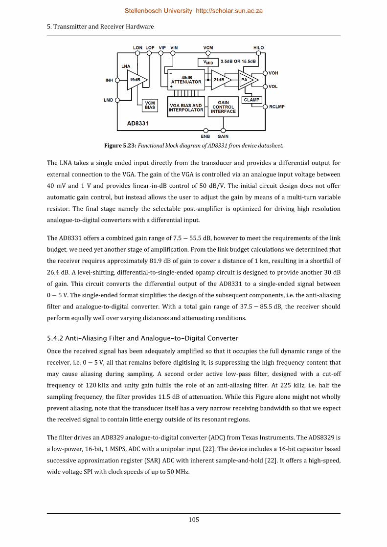
5. Transmitter and Receiver Hardware
105
Figure 5.23: Functional block diagram of AD8331 from device datasheet.
The LNA takes a single ended input directly from the transducer and provides a differential output for
external connection to the VGA. The gain of the VGA is controlled via an analogue input voltage between
40 mV and 1 V and provides linear-in-dB control of 50 dB/V. The initial circuit design does not offer
automatic gain control, but instead allows the user to adjust the gain by means of a multi-turn variable
resistor. The final stage namely the selectable post-amplifier is optimized for driving high resolution
analogue-to-digital converters with a differential input.
The AD8331 offers a combined gain range of , however to meet the requirements of the link
budget, we need yet another stage of amplification. From the link budget calculations we determined that
the receiver requires approximately 81.9 dB of gain to cover a distance of 1 km, resulting in a shortfall of
26.4 dB. A level-shifting, differential-to-single-ended opamp circuit is designed to provide another 30 dB
of gain. This circuit converts the differential output of the AD8331 to a single-ended signal between
. The single-ended format simplifies the design of the subsequent components, i.e. the anti-aliasing
filter and analogue-to-digital converter. With a total gain range of , the receiver should
perform equally well over varying distances and attenuating conditions.
5.4.2 Anti-Aliasing Filter and Analogue-to-Digital Converter
Once the received signal has been adequately amplified so that it occupies the full dynamic range of the
receiver, i.e. , all that remains before digitising it, is suppressing the high frequency content that
may cause aliasing during sampling. A second order active low-pass filter, designed with a cut-off
frequency of 120 kHz and unity gain fulfils the role of an anti-aliasing filter. At 225 kHz, i.e. half the
sampling frequency, the filter provides 11.5 dB of attenuation. While this Figure alone might not wholly
prevent aliasing, note that the transducer itself has a very narrow receiving bandwidth so that we expect
the received signal to contain little energy outside of its resonant regions.
The filter drives an AD8329 analogue-to-digital converter (ADC) from Texas Instruments. The ADS8329 is
a low-power, 16-bit, 1 MSPS, ADC with a unipolar input [22]. The device includes a 16-bit capacitor based
successive approximation register (SAR) ADC with inherent sample-and-hold [22]. It offers a high-speed,
wide voltage SPI with clock speeds of up to 50 MHz.
Stellenbosch University http://scholar.sun.ac.za

5. Transmitter and Receiver Hardware
106
The sample conversion rate is controlled via an output-compare timer of the PIC32MX that outputs pulses
at 450 kHz on the dedicated conversion-start line of the ADS8329. Once the conversion process is
complete, the sample value is transferred to the PIC32MX via the SPI at a clock speed of 40 MHz.
5.4.3 PIC32MX Buffer
The operation of the PIC32MX buffer corresponds closely to that as described in the transmitter section.
The hardware layout is identical, but the software implementation differs somewhat. The same dual
interchanging queue structure now serves to record sample values from the ADC and in turn despatching
the values to the USB-SPI interface. Sample values are recorded at 450 kHz via the PIC32MX’s second SPI
channel and saved to the queue. Once a queue has been filled, recording switches to the alternate queue
and values from the full queue is despatched via the first SPI channel to the USB-SPI interface in blocks of
32 k samples. The process is governed by means of timed interrupts and indicator flags that determine
the status of each queue.
5.4.4 USB-SPI Interface
As with the PIC32MX buffer, the USB-SPI interface operates identically to its counterpart in the
transmitter. The FTDI FT2232H UBS-to-multipurpose-UART acts as the master device, transferring blocks
of 32 k sample values from the PIC32MX buffer at 30 MHz. The SPI-to-USB translation occurs seamlessly
and the data is immediately available in the command stack of the device. Access to the command stack of
the FT2232H is facilitated through the provided DLL. Synchronisation between the PIC32MX buffer and
the FT2232H takes place via a general purpose input-output line that signals the FT2232H that a queue
has been filled and is ready to be dispatched.
Sample values from the command stack of the FT2232H are recorded to a file on the computer’s hard disk
drive in a raw binary format. The Matlab algorithm can later read the received signal from the disk for
demodulation.
5.5 Summary
Through our investigation into acoustic underwater transducers, we realise that these are fairly limiting
devices, especially when it comes to bandwidth. While wideband devices are available at a high cost, we
have to make do with low-cost, narrowband Furuno 520-5PSD transducers. A lot of effort is spent on
characterising these devices in order to predict its frequency response, so that we may apply pre-
emphasis to the transmitted signal to gain a sufficiently flat response. We progress to a link budget
calculation that indicates the required gain figures for the analogue components of the electronic
hardware. A brief description of the function and design of each of the hardware modules is given. Note
that the hardware is only tasked with playback and/or recording of signals and that other than
reconstruction and anti-aliasing filtering, these components do not contribute to the signal processing of
the modem. In the next chapter we evaluate the complete system by putting it to the test in a practical
scenario.
Stellenbosch University http://scholar.sun.ac.za

107
6 PRACTICAL TESTS AND SYSTEM EVALUATION
The ultimate confirmation of the success of any design lies in its performance when subjected to rigorous
testing. In this chapter we set out to conduct a number of practical tests that will confirm the successful
design of the prototype modem. Adhering to general scientific methodology, we start off by identifying
those aspects of the system that need to be assessed and we set corresponding objectives against which
the results will be measured. In order to avoid coincidences, emphasis is placed on the consistency and
repeatability of test results. We discuss the test setup and conditions under which testing was carried out.
A conscientious analysis of the results is performed and we conclude that the design is successful even
though the test conditions presented some shortcomings.
6.1 Objectives of Testing
The objectives of this project broadly state that a scalable communication link is to be established that is
capable of covering a significant distance, is robust against the distorting effects of the underwater
channel and can deliver a reasonable data rate. To determine the degree of success with which these
requirements were met, we investigate various key facets of the system that contribute to its overall
performance.
6.1.1 Hardware Verification
Our first and foremost goal is to successfully transmit and receive a recognizable acoustic signal to
confirm the proper operation of the hardware. We aim to verify the successful transfer of the signal
between the computer and digital hardware without a loss of integrity, the translation of the signal
between its digital and analogue equivalents and lastly the performance of the analogue components
from the power amplifier, low-noise preamplifier and filters.
6.1.2 Accuracy of Amble Extraction
With the full operation of the hardware confirmed, we proceed onto the performance of the modulation
scheme. Our main concern here lies with the accuracy of the timing and frequency synchronisation and
the channel estimation processes. The OFDM modulation scheme relies heavily on the precise extraction
of the pre- and postamble symbols of each frame. We investigate the accuracy with which the timing of
amble symbols can be determined. The emphasis here is on repeatability; if we can attain consistent
results across a number of consecutive frames, the peak detection technique can be deemed successful.
Closely related to the timing synchronisation, is the frequency synchronisation. We investigate the
performance of the cubic spline interpolation method as a means of sample rate conversion to
compensate for Doppler frequency shifts. The rotational spreading of demodulated QAM-symbols on a
constellation diagram serves as an undeniable indication of any residual frequency mismatches.
Stellenbosch University http://scholar.sun.ac.za

6. Practical Tests and System Evaluation
108
6.1.3 Accuracy of Channel Estimation
Through channel estimation and equalisation we aim to determine the influence of the channel on the
received signal and to compensate for its distorting effects. Without prior knowledge of the anticipated
channel however, it becomes problematic to judge the accuracy of the channel estimation process. A
scatter plot of the received QAM-symbols on a constellation diagram does provide some means of
identifying deficiencies in the channel estimate. Additive noise and unpredictable distortions of the
received QAM-symbols appears to randomly scatter the symbols, while errors in the channel estimate
manifest as discernable distortion patterns in the scatter plot. For instance, a frequency dependent
rotation of the symbols about the centre of the constellation would indicate that the phase response of the
channel estimate failed to accurately predict the effects of a residual frequency mismatch. To identify
such patterns we again rely heavily on the consistency of the results across multiple OFDM symbols. If the
distortions are recurrent, we are dealing with a predictable effect that should be included in the channel
estimation. If the distribution of symbols is purely random, we can confirm that the channel estimate
successfully compensates for all predictable influences on the signal.
6.1.4 Link Quality and Error Control Performance
The ultimate measure of the quality of a communication link is certainly the achievable signal-to-noise
ratio. Additive noise and unpredictable distortions disrupt the received QAM-symbols so that a degree of
uncertainty about its original position on the constellation diagram remains after equalisation. We
determine the SNR of the signal by calculating the distance between the received symbols and its original
positions and relate this error magnitude to the overall signal power. The SNR dictates the trade-off
between the reliability and information rate of the channel. At a given information rate, an increase in the
SNR will improve the reliability of the communication link. Alternatively the information rate may be
increase without sacrificing reliability. This forms the basis of adjustable modulation techniques where
the quality of the link is optimally utilised to maximise the data throughput while maintaining its
reliability. The resulting SNR also serves as a gauge to compare the performance of different channel
estimation and equalisation techniques that are investigated.
Our final inquiry is into the symbol and bit error performance of the system. We investigate the
occurrence of symbol and bit errors and compare the results with the theoretically expected values at a
given SNR. We also verify the uniform distribution of bit errors across the codewords of a frame to
confirm the efficiency of the proposed cyclically shifting interleaving scheme. Finally, the abilities of the
BCH error correction codes are put to the test to determine its aptness in the underwater environment.
6.2 The Test Setup and Conditions
Ideally the field testing of any system should be conducted under conditions that closely match the real
world environment in which it would find application. For our modem, such an environment would
preferably be in the ocean, perhaps in a sizeable harbour that is large enough to allow for
communications over a distance of up to 1 km. A few reflective surfaces to present multiple propagation
paths, together with some ambient mechanical noise and the odd shoal of fish to obstruct the signal path
Stellenbosch University http://scholar.sun.ac.za
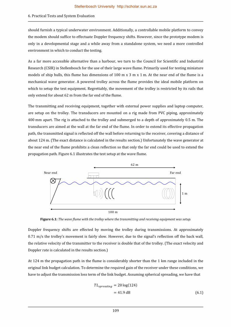
6. Practical Tests and System Evaluation
109
should furnish a typical underwater environment. Additionally, a controllable mobile platform to convey
the modem should suffice to effectuate Doppler frequency shifts. However, since the prototype modem is
only in a developmental stage and a while away from a standalone system, we need a more controlled
environment in which to conduct the testing.
As a far more accessible alternative than a harbour, we turn to the Council for Scientific and Industrial
Research (CSIR) in Stellenbosch for the use of their large wave flume. Primarily used for testing miniature
models of ship hulls, this flume has dimensions of 100 m x 3 m x 1 m. At the near end of the flume is a
mechanical wave generator. A powered trolley across the flume provides the ideal mobile platform on
which to setup the test equipment. Regrettably, the movement of the trolley is restricted by its rails that
only extend for about 62 m from the far end of the flume.
The transmitting and receiving equipment, together with external power supplies and laptop computer,
are setup on the trolley. The transducers are mounted on a rig made from PVC piping, approximately
400 mm apart. The rig is attached to the trolley and submerged to a depth of approximately 0.5 m. The
transducers are aimed at the wall at the far end of the flume. In order to extend its effective propagation
path, the transmitted signal is reflected off the wall before returning to the receiver, covering a distance of
about 124 m. (The exact distance is calculated in the results section.) Unfortunately the wave generator at
the near end of the flume prohibits a clean reflection so that only the far end could be used to extend the
propagation path. Figure 6.1 illustrates the test setup at the wave flume.
Figure 6.1: The wave flume with the trolley where the transmitting and receiving equipment was setup.
Doppler frequency shifts are effected by moving the trolley during transmissions. At approximately
.7 m/s the trolley’s movement is fairly slow. However, due to the signal’s reflection off the back wall,
the relative velocity of the transmitter to the receiver is double that of the trolley. (The exact velocity and
Doppler rate is calculated in the results section.)
At 124 m the propagation path in the flume is considerably shorter than the 1 km range included in the
original link budget calculation. To determine the required gain of the receiver under these conditions, we
have to adjust the transmission loss term of the link budget. Assuming spherical spreading, we have that
( )
(6.1)
100 m
1 m
62 m
Near end Far end
Stellenbosch University http://scholar.sun.ac.za
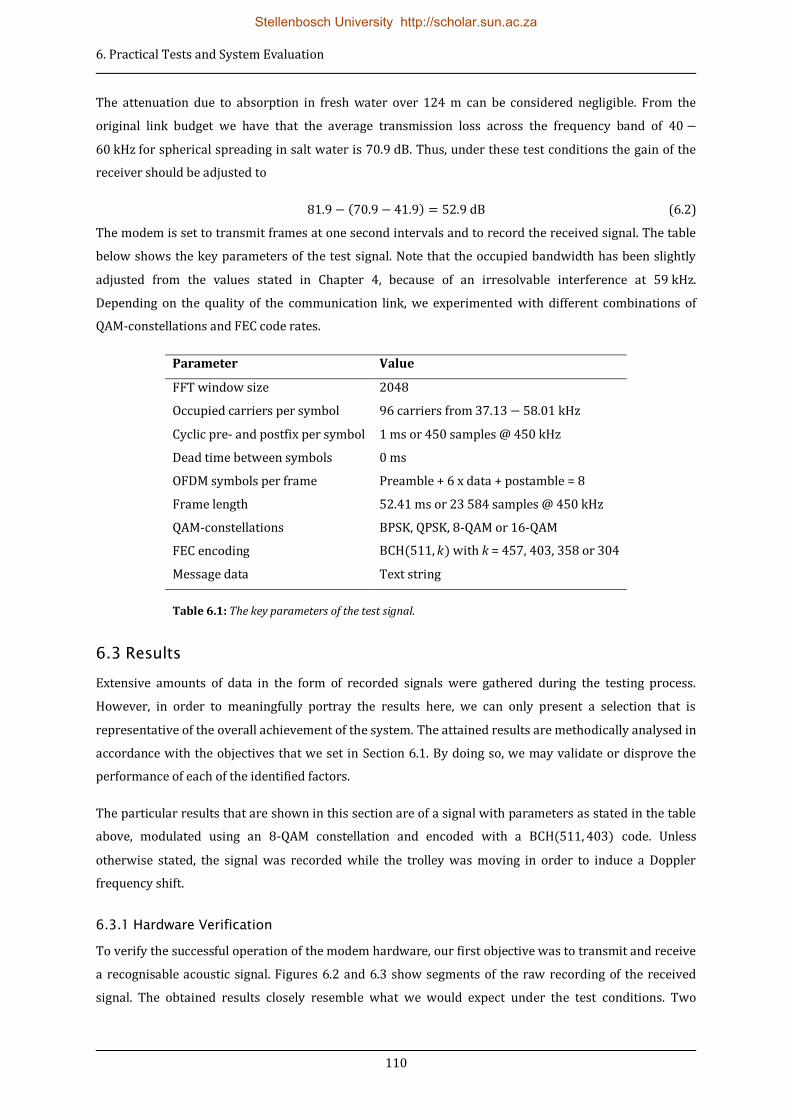
6. Practical Tests and System Evaluation
110
The attenuation due to absorption in fresh water over 124 m can be considered negligible. From the
original link budget we have that the average transmission loss across the frequency band of
for spherical spreading in salt water is 70.9 dB. Thus, under these test conditions the gain of the
receiver should be adjusted to
( ) (6.2)
The modem is set to transmit frames at one second intervals and to record the received signal. The table
below shows the key parameters of the test signal. Note that the occupied bandwidth has been slightly
adjusted from the values stated in Chapter 4, because of an irresolvable interference at 59 kHz.
Depending on the quality of the communication link, we experimented with different combinations of
QAM-constellations and FEC code rates.
Parameter Value
FFT window size 2048
Occupied carriers per symbol 96 carriers from
Cyclic pre- and postfix per symbol 1 ms or 450 samples @ 450 kHz
Dead time between symbols 0 ms
OFDM symbols per frame Preamble + 6 x data + postamble = 8
Frame length 52.41 ms or 23 584 samples @ 450 kHz
QAM-constellations BPSK, QPSK, 8-QAM or 16-QAM
FEC encoding ( ) with k = 457, 403, 358 or 304
Message data Text string
Table 6.1: The key parameters of the test signal.
6.3 Results
Extensive amounts of data in the form of recorded signals were gathered during the testing process.
However, in order to meaningfully portray the results here, we can only present a selection that is
representative of the overall achievement of the system. The attained results are methodically analysed in
accordance with the objectives that we set in Section 6.1. By doing so, we may validate or disprove the
performance of each of the identified factors.
The particular results that are shown in this section are of a signal with parameters as stated in the table
above, modulated using an 8-QAM constellation and encoded with a ( ) code. Unless
otherwise stated, the signal was recorded while the trolley was moving in order to induce a Doppler
frequency shift.
6.3.1 Hardware Verification
To verify the successful operation of the modem hardware, our first objective was to transmit and receive
a recognisable acoustic signal. Figures 6.2 and 6.3 show segments of the raw recording of the received
signal. The obtained results closely resemble what we would expect under the test conditions. Two
Stellenbosch University http://scholar.sun.ac.za

6. Practical Tests and System Evaluation
111
versions of each transmitted frame are visible. The first appears to be severely smeared as it is made up of
multiple reflections from the floor, walls and water surface. The second is a much clearer reflection off
the far wall of the flume. A closer inspection of the signal reveals no gross loss of integrity due to sample
value errors, dropped samples or any other faults that might indicate a malfunction of the digital
hardware. As far as the analogue hardware is concerned we commend its low interference levels and the
accuracy with which the signal could be reproduced.
Figure 6.2: A five second segment of the recorded received signal. (Due to the scaled-down resolution of this plot the
noise levels are misleading. Refer to Figure 6.3 for an accurate representation.)
Figure 6.3: The two received versions of each transmitted frame are separated by approximately 84 ms. Note how the
OFDM symbols are severely smeared in the first version, while they are discernible in the reflected version.
6.3.2 Accuracy of Amble Extraction
To assess the accuracy with which the positions of the amble symbols in the received signal can be
determined, we rely on the consistency of the attained results. Figures 6.4 and 6.5 show segments of the
0 1 2 3 4 50
0.5
1
1.5
2
2.5
3
3.5
4
4.5
5
Am
pli
tud
e [
V]
Time t [s]
0.62 0.64 0.66 0.68 0.7 0.72 0.74 0.760
0.5
1
1.5
2
2.5
3
3.5
4
4.5
5
Am
pli
tud
e [
V]
Time t [s]
Stellenbosch University http://scholar.sun.ac.za

6. Practical Tests and System Evaluation
112
cross correlation between the received signal and the known pre- and postamble symbols. Peaks in the
cross correlation correspond to the positions of the amble symbols. These peaks resemble modulated sinc
pulses, so that the peak detection algorithm has to determine the exact centre of the modulated pulse.
Figure 6.6 shows a closer look at the results of the peak detection algorithm.
Figure 6.4: The position of the preamble as determined by identifying peaks in the cross correlation. The detection
threshold was set to include only the peak of the reflected frame.
Figure 6.5: The position of the postamble as determined by identifying peaks in the cross correlation. The detection
threshold was set to include only the peak of the reflected frame.
0.62 0.64 0.66 0.68 0.7 0.72 0.74 0.760
1
2
3
4
5
Time t [s]
Am
pli
tud
e
Cross correlation
Upsampled correlation
Envelope
Peak
Threshold
0.62 0.64 0.66 0.68 0.7 0.72 0.74 0.760
1
2
3
4
5
Time t [s]
Am
pli
tud
e
Cross correlation
Upsampled correlation
Envelope
Peak
Threshold
Stellenbosch University http://scholar.sun.ac.za

6. Practical Tests and System Evaluation
113
Figure 6.6: The results of the peak detection algorithm indicating the exact location of the preamble in the received
frame.
The distances between the pre- and postambles of the five frames in Figure 6.2 are shown in Table 6.2
below. The distances are indicated as a number of samples.
Frame number Number of samples between pre- and postamble peaks
Frame 1 20 656
Frame 2 20 655
Frame 3 20 657
Frame 4 20 656
Frame 5 20 655
Table 6.2: The distance between the preamble and postamble of each of the received frames.
The results are astoundingly accurate with only a single sample deviation from the median value of
20 656 across all five frames.
By comparing the measured frame length with the original length, we are able to calculate the exact
Doppler ratio and from it, the velocity of the trolley. The original distance between the pre- and
postambles is calculated as
( ) ( ) (6.3)
The well-known Doppler equation is given as
(6.4)
with and representing the observed and emitted frequencies, the sound velocity in water and
and the velocities of the receiver and transmitter. The ratio of the measured and the original frame
lengths is equivalent to the ratio of the observed and emitted frequencies so that we may write
0.7004 0.7004 0.7005 0.7005 0.7006 0.70060
1
2
3
4
5
Time t [s]
Am
pli
tud
e
Cross correlation
Upsampled correlation
Envelope
Peak
Threshold
Stellenbosch University http://scholar.sun.ac.za

6. Practical Tests and System Evaluation
114
(6.5)
As the trolley moves away from the far end of the flume, the transmitter and receiver effectively travel in
opposite directions away form each other at exactly the same speed, so that
(6.6)
Substituting equation 6.6 into 6.5 we have that
( )
(6.7)
The speed of sound in fresh water at a temperature of and a depth of 0.5 m is calculated from
equation 2.1 as 1465 m/s. The velocity of the transmitter (and equivalently the trolley) is
( )
(6.8)
The relative velocity between the transmitter and the receiver is thus
( )
⁄ (6.9)
We can also determine the exact length of the propagation path by measuring the time delay between the
directly received and the reflected versions of a received frame. The peak detection threshold is lowered
to include both peaks. The time delay is
(6.10)
The propagation path length is then calculated as
(6.11)
To compensate for the distance between the transducers , we add 0.4 m to the path length.
6.3.3 Accuracy of Channel Estimation
While the least-squares method of channel estimation does not provide the most accurate predictions
possible, we have chosen this method for its simplicity and computational efficiency. In order to assess
the consistency of the channel estimates, we use the results of five frames of a signal that was recorded
under unchanging channel conditions, i.e. from a stationary trolley.
The channel estimates, as determined from the pre- and postambles of the first frame of the signal
segment is shown in Figure 6.7. The amplitude response of the channel exhibits a very wide range of
Stellenbosch University http://scholar.sun.ac.za
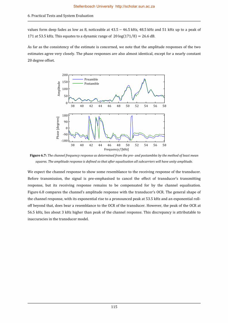
6. Practical Tests and System Evaluation
115
values form deep fades as low as 8, noticeable at , 48.5 kHz and 51 kHz up to a peak of
171 at 53.5 kHz. This equates to a dynamic range of ( ⁄ ) .
As far as the consistency of the estimate is concerned, we note that the amplitude responses of the two
estimates agree very closely. The phase responses are also almost identical, except for a nearly constant
20 degree offset.
Figure 6.7: The channel frequency response as determined from the pre- and postambles by the method of least mean
squares. The amplitude response is defined so that after equalisation all subcarriers will have unity amplitude.
We expect the channel response to show some resemblance to the receiving response of the transducer.
Before transmission, the signal is pre-emphasised to cancel the effect of transducer’s transmitting
response, but its receiving response remains to be compensated for by the channel equalisation.
Figure 6.8 compares the channel’s amplitude response with the transducer’s OCR. The general shape of
the channel response, with its exponential rise to a pronounced peak at 53.5 kHz and an exponential roll-
off beyond that, does bear a resemblance to the OCR of the transducer. However, the peak of the OCR at
56.5 kHz, lies about 3 kHz higher than peak of the channel response. This discrepancy is attributable to
inaccuracies in the transducer model.
38 40 42 44 46 48 50 52 54 56 580
50
100
150
200
Am
pli
tud
e
38 40 42 44 46 48 50 52 54 56 58
-180
-90
0
90
180
Ph
ase
[d
egr
ees]
Frequency f [kHz]
Preamble
Postamble
Stellenbosch University http://scholar.sun.ac.za

6. Practical Tests and System Evaluation
116
Figure 6.8: The amplitude response of the channel compared to the OCR of the transducer. The OCR is scaled to have the
same maximum amplitude as the channel.
An interesting phenomenon is observed when we compare the channel estimates obtained from all five
frames. Figure 6.9 shows the frequency responses as determined from the five consecutive frames. The
respective amplitude responses of the pre- and postambles agree so closely that it is barely discernable
on the Figure. The fact that the preambles show such a high level of consistency between different frames,
but that it differs from the postambles indicate that the signal suffers from a distortion that is dependant
on its specific waveform. This type of distortion is attributable to non-linearities in the signal path.
Factors such as cross-over distortion, insufficient slew rates, clipping and the non-linear efficiency of
transducers all contribute to non-linear distortion of the signal.
Figure 6.9: The channel frequency response as determined from the pre- ad postambles of all 5 frames.
While we have confirmed that the channel estimates can be repeated with a high level of consistency, we
are still to prove its reliability. Through an inspection of the equalised QAM symbols on a constellation
38 40 42 44 46 48 50 52 54 56 580
50
100
150
Am
pli
tud
e
Frequency f [kHz]
Preamble
Postamble
Scaled OCR
38 40 42 44 46 48 50 52 54 56 580
50
100
150
200
Am
pli
tud
e
38 40 42 44 46 48 50 52 54 56 58
-180
-90
0
90
180
Ph
ase
[d
egr
ees]
Frequency f [kHz]
Preambles of 5 frames
Postambles of 5 frames
Stellenbosch University http://scholar.sun.ac.za

6. Practical Tests and System Evaluation
117
diagram, we should be able to identify any residual distortions that can indicate shortcomings of the
channel estimation process. Figure 6.10 shows a scatter plot of the equalised symbols from the first frame
of the original Doppler corrected signal. The symbols are grouped by frequency. This plot should reveal
any uncorrected frequency dependant distortions, but instead we find that the symbol distributions are
completely random. Outlier symbols tend to appear in the approximate frequency range of .
This corresponds to the region of very low amplitudes in the channel frequency response.
Figure 6.10: A scatter plot of the received symbols on an 8-QAM constellation grouped by frequency.
Figure 6.11 shows the same equalised QAM symbols that are now grouped by OFDM symbol. Again, this
plot reveals no time dependant distortions along the duration of the frame. We may safely assume that
only additive noise and unpredictable distortions remain.
Figure 6.11: A scatter plot of the received symbols on an 8-QAM constellation diagram grouped by OFDM symbol. Note
that symbol 1contains 63 BPSK symbols of the frame header, hence the many blue ±1 symbols.
-1.5 -1 -0.5 0 0.5 1 1.5
-1.5
-1
-0.5
0
0.5
1
1.5
37.1 kHz
39.8 kHz
42.4 kHz
45.0 kHz
47.7 kHz
50.3 kHz
53.0 kHz
55.6 kHz
58.0 kHz
-1.5 -1 -0.5 0 0.5 1 1.5
-1.5
-1
-0.5
0
0.5
1
1.5
Symbol 1
Symbol 2
Symbol 3
Symbol 4
Symbol 5
Symbol 6
Stellenbosch University http://scholar.sun.ac.za

6. Practical Tests and System Evaluation
118
6.3.4 Link Quality and Error Control Performance
The quality and reliability of a communication link are contingent upon its achievable SNR and error
control performance. Table 6.3 presents a summary of the overall SNR and error rates of the five frames
from the test signal.
Frame number SNR Number of symbol errors Bit errors in three codewords
Frame 1 12.09 dB 11
Frame 2 12.13 dB 14
Frame 3 11.99 dB 14
Frame 4 12.07 dB 14
Frame 5 11.97 dB 12
Table 6.3: The SNR and error rates of the received signal.
The overall symbol error rate, calculated from the results above, is
(6.12)
From the simulation results in Chapter 3 have that the SER for the optimal 8-QAM constellation at an SNR
of 12 dB is or approximately . This value is applicable for additive white Gaussian
noise. At , the measured SER is slightly higher that anticipated. This can be attributed to the
distribution of QAM-symbols that does not perfectly obey a Gaussian distribution. The majority of
symbols errors are caused by a few outliers that do not contribute significantly to the degradation of the
SNR.
The overall bit error rate is calculated as
(6.13)
Again the measured result exceeds the simulated BER of or approximately at an
SNR of 12 dB. This is expected because of the higher SER.
The ratio of bit errors to symbols errors of confirms the claim in Chapter 3 that four bit
errors occur for every three symbol errors on an optimal 8-QAM constellation.
Stellenbosch University http://scholar.sun.ac.za

6. Practical Tests and System Evaluation
119
As far as the distribution of bit errors among codewords are concerned, we note that the average ratio of
bit errors among the three parallel codewords per frame is . This result confirms the efficiency
of the cyclic shifting interleaving scheme to uniformly distribute bit errors among the codewords.
The data in the frames is encoded by a ( ) code, capable of correcting up to 12 bit errors per
codeword. With three codewords per frame and the given bit error rate, the anticipated frame error rate
is or approximately 1/54. This reliability rapidly increases for lower code rates.
The effective data throughput of the test signal, using 8-QAM and ( ) and including all
overhead, is calculated as
( ) ( )
(6.14)
6.4 Conclusion
We could confirm the successful operation of the digital components of the modem hardware, but the
non-linear distortions that appeared in the channel estimates give cause for concern. Although not
definitively proved, the origin of this distortion probably lies with the power amplifier. It could however,
also be caused by any of the analogue components in the signal chain. The rectification of this problem
should significantly improve the quality of the communication link. Further investigation is
recommended.
Astoundingly consistent results were attained for the accuracy of the amble extraction process. The
Doppler frequency shift could be precisely determined and corrected for by the cubic spline sample rate
conversion method. Any residual subsample-length timing offsets, which could result in a frequency
dependent phase rotation of the QAM symbols, were perfectly compensated for by the channel
estimation. No predictable distortion effects in the distribution of the QAM symbols could be discerned, so
that the channel estimation may be deemed reliable and accurate.
At an overall SNR of approximately 12 dB, the modem proved to be exceedingly reliable for BSPK and
QPSK modulation, with almost no symbol errors ever encountered. With 8-QAM, the number of symbol
errors is more significant so that the BCH error correction codes were properly put to the test. We
confirm that the choice of BCH block codes paired with the cyclically shifting interleaving scheme
performs adequately to provide a reliable communication link. Unfortunately, the SNR is too low to
demodulate a 16-QAM signal with sufficient reliably.
In general, the performance of prototype modem proved the design to be very successful. Even though the
test setup was somewhat limiting in the maximum attainable range and the speed of platform, we can be
confident that the system should perform satisfactorily in a real world environment.
Stellenbosch University http://scholar.sun.ac.za

120
7 CONCLUSION AND FUTURE WORK
At the beginning of this project we set out to investigate the viability of an underwater acoustic modem
using OFDM as modulation scheme. The underwater environment sets significant challenges to overcome
if a reliable acoustic communication link is to be established. Long delay spreads due to multipath
propagation, severe Doppler frequency shifts, frequency selective absorption and very limited bandwidth
are but some of the challenges to overcome. OFDM was proposed as a suitable modulation technique to
meet these challenges. It accomplishes the parallel transmission of data on multiple subcarriers at closely
spaced frequencies. The resulting low parallel symbol rate renders the signal robust against intersymbol
interference. However, because of the close proximity of subcarriers the signal is prone to intercarrier
interference caused by Doppler frequency shifts.
We devised a method of using preamble and postamble symbols to facilitate the accurate timing and
frequency synchronisation of the signal. The amble symbols serve a dual purpose in that it is also used for
channel estimation. The modulation scheme, employing optimal QAM-constellations and BCH forward
error correction codes, is wholly defined in software. The software scripts are implemented in Matlab, but
it only provides off-line processing of the transmittable and received signals. The electronic hardware of
the modem provides a versatile platform to transmit pre-generated signals and to record received signals.
It was specifically designed not to impose limitations on the specifications of the modulation scheme. We
performed an in-depth analysis of the transducers that is used with the modem. Although these were
found not be ideal for broadband communications, we were able to successfully employ it in the design.
The modem was tested under somewhat limiting condition in a wave flume, but the attained results were
exceedingly satisfying. We succeeded in proving the concept of acoustic underwater communication via
OFDM modulation.
7.1 Future Work
As with any proof-of-concept design, many possible improvements remain to be made to the modem. The
most immediate and perhaps least invasive of these pertain to the software defined modulation scheme.
The channel estimation performance may be improved by implementing a more robust estimation
method than the current least-squares estimator. The structure of OFDM lends itself to the placement of
pilot symbols at different time and frequency intervals. This allows for very powerful estimation methods
that could significantly increase the channel quality. Furthermore, the addition of a decision feedback
loop, where demodulated data-carrying symbols are used to improve the channel estimate, should also be
considered.
Related to this is the question of hard versus soft decision demodulation techniques. Currently, the
received QAM-symbols are demodulated as either one symbol or another without any consideration of
the certainty of that decision. If more symbol errors occur than what could be corrected by the FEC code,
Stellenbosch University http://scholar.sun.ac.za

7. Conclusion
121
a codeword is simply deemed unrecoverable. However, if it was possible to re-evaluate the decisions of
symbols that lie close to a boundary, we might yet be able to correct the codeword. This forms the basis of
the Viterbi algorithm. The implementation of a soft decision demodulation scheme should significantly
improve the reliability of the communication channel.
Possible improvements to the hardware of the modem include the use of omnidirectional, broadband
transducers that are specifically designed for communication purposes. The Reson model TC1026 and
Neptune Sonar model T257 are good examples of such devices. Further more, an upgrade to a highly
linear, wideband power amplifier to drive the transducer should solve the non-linear distortions
observed during the testing.
The ultimate final product would be a standalone modem capable of bi-directional communications
ready for deployment in an undersea sensor network, a remotely operated submarine or whatever other
application it could be used for. Its modulation scheme would be implemented on a field programmable
gate array (FPGA) or similar processing unit capable of performing the signal processing in real-time.
Such a modem will also feature fully variable modulation capabilities and might even include multiple-
input multiple-output (MIMO) technology to improve the reliability of the communication link.
Stellenbosch University http://scholar.sun.ac.za
122
REFERENCES
[1] F.I. Gonzales et al., “Deep-ocean Assessment and Reporting of Tsunamis (DART) - Brief Overview
and Status Report,” Pacific Marine Environmental Laboratory of the National Oceanic and
Atmospheric Administration, Seattle, 1998
[2] H.G. Urban, Handbook of Underwater Acoustic Engineering, Bremen, Germany: STN ATLAS
Elektronik GmbH, 2002
[3] H. Schulze and C. Lüders, Theory and Application of OFDM and CDMA, West Sussex, England: John
Wiley and Sons Ltd., 2005
[4] T.D. Rossing (Editor), “Underwater Acoustics,” in Springer Handbook of Acoustics, New York:
Springer Science+Business Media, 2007
[5] J.A. Ogilvy, Wave scattering from rough surfaces, UK: IOP Publishing, 1987
[6] F.H. Fisher and V.P. Simons, “Sound Absorption in Sea Water,” J. Acous. Soc. Am., Vol. 62, No. 3,
Sep. 1977
[7] T.S. Rappaport, “Doppler Spread and Coherence Time, ” in Wireless Communications: Principles
and Practice, 2nd ed. Prentice Hall, 2007
[8] R.W. Chang, “Synthesis of Band-Limited Orthogonal Signals for Multichannel Data Transmissio,”
Bell Systems Tech. J., Vol. 45, Dec. 1960
[9] S.B. Weinstein and P.M. Ebert, “Data Transmission of Frequency Division Multiplexing Using the
Discrete Frequency Transform,” IEEE Trans. On Communications, Vol. COM-19, No. 5, Oct. 1971
[10] J.G. Proakis and D.G. Manolakis, Digital Signal Processing Principles, Algorithms and Applications,
4th ed., New Jersey, Pearson Prentice Hall, 2007
[11] S. McKinley and M. Levine. (1998). Cubic Spline Interpolation.[Online]. Available:
http://online.redwoods.cc.ca.us/instruct/darnold/laproj/fall98/skymeg/proj.pdf
[12] Y. Shen and E. Martinez, “Channel Estimation in OFDM Systems,” Freescale Semiconductor, 2 6
[13] E. Kuntsal and W.A. Baunker, “Guidelines for Specifying Underwater Electroacoustic
Transducers,” in UDT ’92 Conference, London, 1992
[14] W.W.L. Au and M.C. Hastings, Principles of Marine Bioacoustics, New York: Springer
Science+Business Media, 2008
[15] Furuno USA. (2011, Des. 1). Product detail 520-5PSD [Online]. Available:
http://www.furunousa.com
Stellenbosch University http://scholar.sun.ac.za

References
123
[16] Datasheet of FT2232H Dual High Speed USB to Multipurpose, Future Technology Devices
International Ltd., Glasgoe, 2009.
[17] Datasheet of dsPIC33FJ12GP201/202 High Performance 16-bit Digital Signal Controller, Microchip
Technology Inc., 2009
[18] Datasheet of DAC8830 16-bit, Ultra-Low Power, Voltage-Output Digital-to-Analogue Converter,
Texas Instruments, 2007
[19] Datasheet of LM3886 Overture Audio Power Amplifier Series, National Semiconductor, 2003
[20] B.P. Lathi, Modern Digital and Analogue Communication Systems, 3rd ed., New York, Oxford
University Press, Inc., 1998
[21] Datasheet of AD8833 Ultra-Low Noise VGA’s with Preamplifier and Programmable Rin, Analog
Devices, Norwood, 2008
[22] Datasheet of AD8329 Low-Power, 16-bit, 1 MHz, Single/Dual Unipolar Input, Analog-to-Digital
Converter with Serial Interface, Texas Instruments, 2009
Stellenbosch University http://scholar.sun.ac.za
Top Related