


Languages
Pages
Legal


An Analysis of a Sea Breeze Boundary in
Florida
James Brownlee
Florida Institute of Technology
Department of Marine and Environmental Systems

Outline of Talk
• Introduction to Sea Breezes • Radar and Sea Breeze Detection• Goals of this study• Methods and the area where the June 12th Sea Breeze was
captured• Analysis of Radar, Satellite, and Ground Observations of the
Sea Breeze• Insects or Clouds?• Conclusion/Implications

Introduction
• What is a sea breeze?• An onshore wind that develops along the coastline.• It is driven by the temperature contrast between the land and
sea.• Sea Breeze Circulations can reach 50 to 100 km horizontally.
• Vertically they typically reach 300 to 700 meters.

Figure 1: A “ideal” diagram of a sea breeze circulation. (Image taken from NWS Jetstream)

Figure 2: This shows the horizontal and vertical dimensions of a sea breeze circulation. (Image taken from Tijm et al., 1999)
Ocean Land

Radar Observations of Sea Breezes
• Radar is typically used to detect areas of precipitation, but it can also detect echoes that are not due to clouds or precipitation.
• Such radar returns are known as clear air echoes.
• Radar thin lines associated with sea breezes are a very common example of a clear air echo returns.
• Much debate exists over what causes these radar thin lines.

Questions/Goals
• Question 1: Is the sea breeze thin line that is observed on radar represent where the surface boundary is located?
• Question 2: What is responsible for the radar observed thin line that is associated with the sea breeze boundary?
• These two questions were addressed while tracking the sea breeze boundary on June 12th.

June 12th Sea Breeze Study
On June 12th, the sea breeze was sampled using the AIRMAR PB 200 weather sensor.
It was tracked on the ground from Melbourne to Kissimmee.
This tracking started at 12:34 PM and ended at 5:54 PM.
A final combination of these ground observations along with radar and satellite imagery were used to analyze this sea breeze boundary.

• Figure 3: This is the AIRMAR sensor that was used capture the sea breeze passage.

• Figure 4: This shows how far inland the sea breeze went (Image taken from Google Maps).
50 km

Ground and Radar Observations of the Sea Breeze.
Figure 5: At 3:05 PM, the sea breeze boundary passed the van as it was stationary along US-192.
18:40:0318:43:3918:47:1518:50:5118:54:2718:58:0319:01:3919:05:1519:08:5119:12:2719:16:0319:19:3919:23:1519:26:5119:30:2719:34:0319:37:39
-3
-2
-1
0
1
2
3
Sea Breeze Passage at 3:05 PM
Time (UTC)
U c
omp
onen
t of
th
e w
ind
in m
/s

Figure 6: This is a radar image of the radar thin line taken at 3:05 PM. The red arrow indicates the location of the thin line. This image was captured at a radar elevation angle of 0.48 degrees.
Radar Thin Line

• Figure 7: This shows the horizontal distance between where the van and the radar saw the sea breeze boundary at 3:05 PM.
19 Kilometers
Van Location
Thin Line Location

• Figure 8: This shows how far apart radar and surface observations of the sea breeze boundary are. AGL = above ground level SB = sea breeze
0 5 10 15 200
0.1
0.2
0.3
0.4
0.5
0.6
0.7
0.8
Surface and Radar Observations of the Sea Breeze Front at 3:05 PM
Horizontal Distance (km)
Verti
cal H
eigh
t (km
)
Radar Observed SB: 19.2 km east; 0.5 km AGL
Radar Observed SB: 19.7 km east; 0.7 km AGL
Radar Observed SB: 18.7 km east; 0.2km AGL
Ground Observation of SB
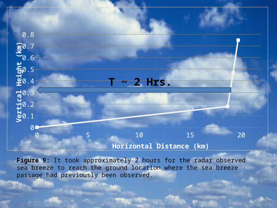
Figure 9: It took approximately 2 hours for the radar observed sea breeze to reach the ground location where the sea breeze passage had previously been observed.
0 5 10 15 200
0.1
0.2
0.3
0.4
0.5
0.6
0.7
0.8
Horizontal Distance (km)
Verti
cal H
eigh
t (km
)
T ~ 2 Hrs.

Insects or Clouds?
• Figure 10: Radar scan of the sea breeze thin line at 5:29 PM. This was taken at an elevation angle of 0.47 degrees.
Radar Thin Line

• Figure 11: Differential reflectivity radar scan at 5:29 PM. This image was captured at an elevation angle of 0.50 degrees.
Radar Thin Line
Thunderstorms

• Figure 12: 1 km resolution visible satellite image captured at 5:31 PM.
Little Cloud Development

• Figure 13
0 5 10 15 200
0.1
0.2
0.3
0.4
0.5
0.6
0.7
0.8
Horizontal Distance (km)
Verti
cal H
eigh
t (km
)
Is this actually the sea breeze boundary?

Figure 14: (Image taken from NWS Jetstream)
Possible Location of the Thin Line

Conclusion and Implications
• The results of this study suggest three things:
• 1. This study shows that there can be a large horizontal distance between ground and radar observations of a sea breeze boundary.
• 2. The radar thin line may have been caused by insects.
• 3. The radar thin line may not mark the true location of the sea breeze boundary near the surface or aloft.
Acknowledgments
• Thanks to Mr. Splitt for his guidance on this project.
• Robby, for all the van driving.
• The Department of Marine and Environmental Systems at FIT for funding this project.

Questions?

References
Abbs, J. A. and W. L. Physick. Sea-breeze observations and modeling: a review. Aust. Met. Mag., 41: 7-19, 1992.•
Atkins, N. T. and R. M. Wakimoto. Influence of the Synoptic-Scale Flow on Sea Breezes Observed during CaPE. Mon. Wea. Rev., 125: 2112-2130, 1997.•
Atkins, N. T., R. M. Wakimoto, and T. M. Weckwerth. Observations of the Sea-Breeze Front during CaPE. Part II: Dual-Doppler and Aircraft Analysis. Mon. Wea. Rev., 123: 944-969, 1995.
Google. Google Maps. 2012. Web. 27 June 2012. <https://maps.google.com/maps?hl=en>

Google. Google Maps. 2012. Web. 27 June 2012. <https://maps.google.com/maps?hl=en>
Simpson, J. E. Sea Breeze and Local Wind. Cambridge University Press, Cambridge/New York/Melbourne, 234 pp., 1994.
Sharp, J. Clear-air Radar Observations and their Application in Analysis of Sea Breezes. University of Washington: Department of Atmospheric Sciences. 1997. 28 June 2012. http://www.atmos.washington.edu/~justin/radar_project/introduc.htm
“The Sea Breeze”. NWS Jet Stream. 13 Jul. 2012 Web. 15 Jul. 2012.
Tijm, A. B. C., A. A. M. Holtslay., and A. J. Van Delden. Observations and Modeling of the Sea Breeze with the Return Current. Mon. Wea. Rev., 127: 625-640, 1999.
Top Related