arX

iv:1

411.

1065

v1 [

astr

o-ph

.GA

] 4

Nov

201

4Draft version July 18, 2021Preprint typeset using LATEX style emulateapj v. 5/2/11

EARLY SCIENCE WITH THE LARGE MILLIMETER TELESCOPE: EXPLORING THE EFFECT OF AGNACTIVITY ON THE RELATIONSHIPS BETWEEN MOLECULAR GAS, DUST, AND STAR FORMATION

Allison Kirkpatrick1, Alexandra Pope1, Itziar Aretxaga2, Lee Armus3, Daniela Calzetti1, George Helou4,Alfredo Montana2, Gopal Narayanan1, F. Peter Schloerb1, Yong Shi5, Olga Vega2, Min Yun1

Draft version July 18, 2021

ABSTRACT

The molecular gas, H2, that fuels star formation in galaxies is difficult to observe directly. Assuch, the ratio of LIR to L′

CO is an observational estimation of the star formation rate comparedwith the amount of molecular gas available to form stars, which is related to the star formationefficiency and the inverse of the gas consumption timescale. We test what effect an IR luminousAGN has on the ratio LIR/L

′CO in a sample of 24 intermediate redshift galaxies from the 5 mJy

Unbiased Spitzer Extragalactic Survey (5MUSES). We obtain new CO(1-0) observations with theRedshift Search Receiver on the Large Millimeter Telescope. We diagnose the presence and strengthof an AGN using Spitzer IRS spectroscopy. We find that removing the AGN contribution to Ltot

IR

results in a mean LSFIR/L

′CO for our entire sample consistent with the mean LIR/L

′CO derived for a

large sample of star forming galaxies from z ∼ 0 − 3. We also include in our comparison the relativeamount of polycyclic aromatic hydrocarbon emission for our sample and a literature sample of localand high redshift Ultra Luminous Infrared Galaxies and find a consistent trend between L6.2/L

SFIR and

LSFIR/L

′CO, such that small dust grain emission decreases with increasing LSF

IR/L′CO for both local and

high redshift dusty galaxies.

1. INTRODUCTION

Star formation is one of the main internal driving forcesof galaxy evolution, resulting in the chemical enrichmentof a galaxy, the heating of the interstellar medium (ISM),and indirectly, the production of dust through the windsof dying stars. Star formation converts a galaxy’s molec-ular gas into stars through multiple complicated pro-cesses including gas accretion and the collapse and cool-ing of molecular clouds. Although the star formation pro-cess itself is intricate, the overall conversion of gas intostars can be expressed simply by the Schmidt-Kennicutt(SK) law which directly relates the molecular gas con-tent to the star formation rate (SFR) through a power-law equation, ΣSFR ∝ Σα

gas, albeit with significant scat-ter (Schmidt 1959; Kennicutt 1998; Kennicutt & Evans2012).The bulk of the present day stellar mass was formed

at a peak epoch of star formation, from z ∼ 1 − 3(Madau & Dickinson 2014, and references therein). Dur-ing this era, the buildup of stellar mass was dominated bydusty galaxies referred to as Luminous Infrared Galax-ies (LIRGs, LIR = 1011 − 1012L⊙) and Ultra Lumi-nous Infrared Galaxies (ULIRGs, LIR > 1012L⊙) (e.g.,Murphy et al. 2011a). In the past two decades, the spateof far-IR/submillimeter space-based and ground-basedtelescopes have enabled astronomers to simultaneouslystudy the star formation, through infrared (IR) emis-

1 Department of Astronomy, University of Massachusetts,Amherst, MA 01002, USA, kirkpatr@astro.umass.edu

2 Instituto Nacional de Astrofısica, Optica y Electronica, Ap-dos. Postales 51 y 216, C.P. 72000 Puebla, Pue., Mexico

3 Spitzer Science Center, California Institute of Technology,MS 220-6, Pasadena, CA 91125, USA

4 Infrared Processing and Analysis Center, California Instituteof Technology, Pasadena, CA 91125, USA

5 School of Astronomy and Space Science, Nanjing University,Nanjing, 210093, China

sion, and molecular gas, through CO emission, of dustygalaxies out to redshifts of z ∼ 4 (Carilli & Walter 2013,and references therein). The IR luminosity, LIR, is anideal measure of the SFR for dusty galaxies as it is theintegrated emission from the dust, presumably heatedby star formation. On galaxy-wide scales, CO traces themolecular hydrogen which is difficult to observe directly;a conversion factor, αCO, is used to relate the CO lumi-nosity directly to the H2 mass (Bolatto et al. 2013, andreferences therein).In the past few years, a “galaxy main sequence” has

been empirically determined for local and high redshiftgalaxies; a tight relationship holds between SFR and stel-lar mass, and this relationship evolves with redshift (e.g.,Noeske et al. 2007; Elbaz et al. 2011). Galaxies that lieabove the main sequence, that is, galaxies that have anenhanced SFR for a given stellar mass, are designated“starbursts” in this parameter space, as they are thoughtto be undergoing a short-lived burst of star formation,likely triggered by a major merger. The rate at which agalaxy can form stars is limited by the amount of molec-ular gas present. Shi et al. (2011) proposed an extendedSK law which relates the specific star formation rate(ΣSFR/Σgas) to the stellar mass surface density, suggest-ing that the existing stellar population may play a rolein regulating the amount of star formation. The authorsapply their extended SK law to an analytical model ofgas accretion and find that it accurately reproduces thegalaxy main sequence.A dichotomy between starbursts and normal star form-

ing galaxies may also be observed by comparing LIR

with L′CO. First, there may be a “normal” rate of

star formation measured in undisturbed disk galaxiesfor a given amount of molecular gas. Then, thereis an enhanced starburst mode, where a galaxy hasa higher LIR than expected for a given L′

CO, possi-

2

bly triggered by a major merger funneling gas towardsthe inner regions of a galaxy (e.g., Downes & Solomon1998; Solomon & Vanden Bout 2005; Daddi et al. 2010b;Genzel et al. 2010). This dichotomy has a direct effecton the calculation of the H2 mass, since αCO is proposedto be a factor of ∼ 5 lower for starbursting galaxies, dueto significant amounts of CO residing in the inter-cloudmedium. Correctly identifying starbursts is critical forcalculating accurate gas masses.It now appears that every massive galaxy hosts a su-

permassive black hole at the center, implying that allgalaxies have gone through an active galactic nuclei(AGN) phase, and some LIRGs and ULIRGs show signsof concurrent black hole growth and star formation (e.g.,Sajina et al. 2007; Pope et al. 2008; Coppin et al. 2010;Dıaz-Santos et al. 2010; Wu et al. 2010; Petric et al.2011; Kirkpatrick et al. 2012). In the classical pictureof galaxy evolution, a starburst is triggered by a ma-jor merger, and this phase can be followed by an AGNphase, implying that an obscured growing AGN maybe observable during a galaxy’s starburst phase (e.g.,Sanders & Mirabel 1996). If present, an AGN can dra-matically influence the internal evolution of a galaxyby heating the dust, expelling the gas, and ultimatelyquenching the star formation through feedback mech-anisms (e.g., Alexander & Hickox 2012). The effect ofan obscured AGN on the ISM can be probed throughIR observations. In the mid-IR, star forming galaxieshave prominent PAH features arising from photodisso-ciation regions (PDRs), but AGN emission can dilutethese features, leaving a warm dust power-law continuum(Weedman et al. 2004; Siebenmorgen et al 2004). Radi-ation from the AGN can heat the dust in the ISM totemperatures & 100K, producing a significant contribu-tion (& 50%) to the far-IR emission (e.g., Mullaney et al.2011; Kirkpatrick et al. 2012).The degree of scatter in the relationship between LIR

and L′CO, often attributed to the two different modes of

star formation, is possibly affected by the contributionfrom an AGN to LIR. Evans et al. (2001) observe highLIR/L

′CO in QSOs and infer that these ratios might be

boosted by an AGN contribution to LIR. Evans et al.(2006) build on this study by using HCN as a tracer ofstar formation in QSOs. Using IRAS bright galaxies,the authors determine the median HCN/CO ratio fornormal star forming galaxies and use this, combined withLIR/L

′CO and LIR/L

′HCN, to statistically correct LIR of

QSOs for an AGN contribution. An alternate approachis to use LFIR (40-500µm or 42.5-11.5µm) instead ofLIR (8-1000µm), as dust emission in this regime shouldcome primarily from heating by young stars. Xia et al.(2012) conclude that LFIR/L

′CO in a sample of 17 QSOs is

similar to the ratios in local ULIRGs (many of which areknown to host obscured AGN), and Evans et al. (2006)finds high LFIR/L

′CO ratios in QSOs relative to the IRAS

galaxies.In this paper, we build upon observations in the high

redshift and local Universe with a study of intermediateredshift galaxies (z = 0.04− 0.35) from the 5 mJy Unbi-ased Spitzer Extragalactic Survey (5MUSES; P.I. GeorgeHelou). These galaxies have extensive IR data from theSpitzer Space Telescope and Herschel Space Observatory,allowing us to accurately measure LIR and quantify thecontribution from an AGN. We complement the existing

IR data with new CO(1-0) observations from the Red-shift Search Receiver, which has a large bandwidth of38GHz and a resolution of 100km/s, on the Large Mil-limeter Telescope Alfonso Serrano, enabling us to explorehow much of the scatter in the LIR−L′

CO relation is dueto an AGN contribution to LIR. We discuss the detailsof our sample and observations in Section 2, the effectof an AGN on the relationships between LIR, PAHs, andCO(1-0) emission in Section 3, and summarize our find-ings in Section 4.Throughout this paper, we adopt a flat cosmology with

H0 = 71 kms−1 Mpc−1, Ωm = 0.27, and ΩΛ = 0.73.

2. DATA

2.1. 5MUSES Sample

5MUSES is a Spitzer IRS mid-IR spectroscopic surveyof 330 galaxies selected from the SWIRE and Spitzer Ex-tragalactic First Look Survey fields (details in Wu et al.2010). It is a flux limited sample selected at 24µmusing MIPS observations from the Spitzer Space Tele-scope, with S24 > 5mJy. Crucially, 5MUSES is a rep-resentative sample at intermediate redshift (the medianredshift of the sample is 0.14, 1.8 Gyr ago) of galaxieswith LIR ∼ 1010 − 1012L⊙, bridging the gap betweenlarge samples of local star forming galaxies, LIRGs, andULIRGs and high redshift observations of LIRGs andULIRGs. Complete details of the Spitzer data reductionare found in Wu et al. (2010). For the present study, wemake use of the Spitzer IRS short-low (SL) spectroscopy,spanning the range 5.5− 14.5µm.A 24µm selection criteria could potentially bias the

sample towards warmer sources. Magdis et al. (2013)reports the far-IR observations of the 5MUSES sourceswith the Herschel Space Observatory. Of 188 5MUSESsources covered by the observations, 154 (82%) are de-tected at 250µm. The authors also determine that the250µm flux densities of the whole population of galaxiesin the observed field with S24 > 5mJy (the 5MUSES de-tection limit) and that of the 5MUSES sample is drawnfrom the same distribution, indicating that the dust tem-peratures of 5MUSES are not significantly warmer thanother IR luminous galaxies. In Section 3.2, we comparethe 5MUSES sources to high redshift ULIRGs, also se-lected at 24µm, from the GOODS-Herschel survey. Forthe high redshift ULIRGs, Pope et al. (2013) find no dif-ference between 70µm selected sources (∼ 24µm restframe) and submillimeter selected sources in terms ofPAH and CO luminosities. The high redshift ULIRGsin this work are drawn from a larger parent popula-tion of Spitzer IRS sources (Kirkpatrick et al. 2012).Kirkpatrick et al. (2012) find that 97% of GOODS-Herschel sources with a 100µm detection also have a24µm detection, ensuring that for high redshift LIRGsand ULIRGs, a 24µm selection criteria does not bias theselection towards warmer sources.From the 5MUSES sample, we selected 24 sources

that span a range of PAH equivalent widths (EW; cal-culated for the full sample in Wu et al. 2010), as PAHEW is correlated with the mid-IR strength of an AGN(Armus et al. 2007). All 24µm sources have spectro-scopic redshifts determined from fitting the mid-IR spec-tral features. These sources were chosen for a pilotCO(1-0) study specifically because they exhibit a range

3

TABLE 1CO(1-0) Measurements of the 5MUSES sample

ID RA Dec za rmsb FWHM SCO∆vc L′CO

c

(J2000) (J2000) (CO) (mK) (km s−1) (Jy km s−1) (109 Kkm/s pc2)

5MUSES-200 16:12:50.9 +53:23:05.0 0.043 0.70 · · · < 2.53 < 0.215MUSES-179 16:08:03.7 +54:53:02.0 0.053 0.32 348 ± 20 11.3 ± 0.93 1.46 ± 0.125MUSES-169 16:04:08.3 +54:58:13.1 0.064 0.72 306 ± 67 4.47 ± 1.08 0.84 ± 0.205MUSES-105 10:44:32.9 +56:40:41.6 0.068 0.84 251 ± 20 7.19 ± 1.27 1.54 ± 0.275MUSES-171 16:04:40.6 +55:34:09.3 0.078 0.87 345 ± 48 7.60 ± 1.45 2.14 ± 0.415MUSES-229 16:18:19.3 +54:18:59.1 0.082 0.72 386 ± 33 11.3 ± 1.48 3.53 ± 0.465MUSES-230 16:18:23.1 +55:27:21.4 0.084 0.87 305 ± 50 6.38 ± 1.25 2.09 ± 0.415MUSES-234 16:19:29.6 +54:18:41.9 0.100 0.70 217 ± 25 6.24 ± 0.69 2.93 ± 0.335MUSES-132 10:52:06.6 +58:09:47.1 0.117 1.30 181 ± 44 4.28 ± 0.92 2.77 ± 0.605MUSES-227 16:17:59.2 +54:15:01.3 0.134 0.24 247 ± 26 1.17 ± 0.34 1.00 ± 0.295MUSES-141 10:57:05.4 +58:04:37.4 0.140 0.48 203 ± 29 3.06 ± 0.62 2.86 ± 0.585MUSES-158 16:00:38.8 +55:10:18.7 0.145 0.73 458 ± 78 5.17 ± 1.23 5.21 ± 1.245MUSES-225 16:17:48.1 +55:18:31.1 0.145 0.46 400 ± 146 4.52 ± 0.57 4.55 ± 0.575MUSES-273 16:37:31.4 +40:51:55.6 0.189 0.34 241 ± 69 1.81 ± 0.40 3.16 ± 0.695MUSES-136 10:54:21.7 +58:23:44.7 0.204 0.36 477 ± 78 2.30 ± 0.55 4.69 ± 1.115MUSES-294 17:12:32.4 +59:21:26.2 0.210 0.38 · · · < 1.60 < 3.475MUSES-216 16:15:51.5 +54:15:36.0 0.215 0.27 331 ± 60 1.82 ± 0.36 4.14 ± 0.835MUSES-194 16:11:19.4 +55:33:55.4 0.224 0.54 · · · < 2.62 < 6.495MUSES-249 16:22:14.8 +55:06:14.2 0.237 0.41 · · · < 1.72 < 4.805MUSES-250 16:23:13.1 +55:11:11.6 0.237 0.48 599 ± 40 5.56 ± 0.68 15.5 ± 1.895MUSES-275 16:37:51.4 +41:30:27.3 0.286 0.61 950 ± 163 7.77 ± 1.38 32.0 ± 5.685MUSES-313 17:18:52.7 +59:14:32.1 0.322 0.47 · · · < 2.09 < 10.15MUSES-156 15:58:33.3 +54:59:37.2 0.340 0.47 · · · < 2.17 < 12.85MUSES-101 10:41:59.8 +58:58:56.4 0.360 0.32 · · · < 1.34 < 8.91

Sources are ordered by increasing redshift.a Redshift determined by fitting center of CO(1-0) line. Redshift errors scale with S/N, with the typical error of0.0003 corresponding to S/N∼5. For the sources with 3σ upper limits, we list zIR.b The rms is determined over the entire 38GHz spectrum.c 3σ upper limits are listed for six sources where we were not able to detect a line.

of PAH strengths and because the spectroscopic red-shifts are such that we can observe the CO(1-0) transi-tion with the Large Millimeter Telescope (LMT). Thesesources were also selected according to LIR, such thatevery source is observable in a reasonable (. 90 min)amount of time during the LMT Early Science phase.Our sample spans a redshift range of z = 0.04−0.36 andLIR = 1.8 × 1010 − 1.3 × 1012 L⊙. Details are listed inTable 1.

2.2. New LMT Observations

The LMT is a 50m millimeter-wave radio telescopeon Volcan Sierra Negra, Mexico, at an altitude of 4600m(Hughes et al. 2010). The high elevation allows for a me-dian opacity of τ = 0.1 at 225GHz in the winter months.For the Early Science phase, the inner 32.5m of the pri-mary reflector is fully operational. The primary reflec-tor has an active surface and a sensitivity of 7.0 Jy/Kat 3mm. The pointing accuracy (rms) is 3′′ over thewhole sky and 1-2′′ for small offsets (< 10) from knownsources.During March and April 2014, we observed our

24 sources with the Redshift Search Receiver (RSR;Erickson et al. 2007; Chung et al. 2009). The RSR iscomprised of a dual beam, dual polarization systemthat simultaneously covers a wide frequency range of 73-111GHz in a single tuning with a spectral resolution of100km/s. This large bandwidth combined with a highspectral resolution is ideal for measuring the CO inte-grated line luminosities in high redshift sources. In ourintermediate redshift sample, the large bandwidth allowsus to observe the CO(1-0) transition for sources spanninga wide range of redshifts. The beam size of the RSRis frequency dependent, such that θb = 1.155λ/32.5m.

The beam size depends on the frequency of the observedCO(1-0) line, and at the median redshift, z = 0.145, theRSR has a beam size of 22′′.Typical system temperatures ranged from 87 − 106K

during our observations. Weather conditions varied overthe eight nights of observations, with τ = 0.07 − 0.28.All observations were taken at elevations between 40-70

where the gain curve is relatively flat. On source in-tegration times ranged from 5 − 100 minutes and weredetermined by estimating L′

CO from LIR using the av-erage ratio from Carilli & Walter (2013). The integra-tion times were estimated to obtain a > 3σ detectionof the expected integrated line luminosity in each sourceaccording to the LMT integration time calculator. Weobtained > 3σ detections of 17 out of 24 targets. Withthe sole exception of 5MUSES-313, where the requestedon source integration time was not completed, the de-sired rms was reached for all sources. The rms has beencalculated using the full spectrum from 73-111GHz. Welist the rms in Table 1 for each source. There is no cor-relation between rms and S/N, so low CO(1-0) emissionappears to be an intrinsic property of our undetectedsources.Data were reduced and calibrated using DREAMPY

(Data REduction and Analysis Methods in PYthon).DREAMPY is written by G. Narayanan and is usedspecifically to reduce and analyze LMT/RSR data. Itis a complete data reduction package with interactivegraphics. For each observation scan, four distinct spec-tra are produced from the RSR. After applying appro-priate instrumental calibrations from the DREAMPYpipeline, certain frequencies where known instrument ar-tifacts are sometimes present were removed. There areno known bandpass features in the spectral regions where

4

the CO(1-0) lines are expected. For each observation,linear baselines were calculated outside the region of theCO(1-0) line, and the rms estimated from the baseline ofthe full spectrum is used when all data for a given sourceare averaged together to produce the final spectrum. Theaveraging is a weighted average where the weights are setto 1/rms2.We checked whether aperture corrections were

necessary using the empirical relation derived inSaintonge et al. (2011a) and the optical radii fromNASA/IPAC Extragalactic Database. We calculated atmost a 10% aperture correction for our lowest redshiftgalaxies which have the largest angular extent. Given theuncertainty inherent in applying a correction formula, wehave opted not to apply any aperture corrections.From the final spectrum for each source, in units of

antenna temperature, we determined the locations of theCO(1-0) peak by fitting a simple Gaussian to the spec-trum close to the frequency 115.271/(1 + zIR), allowingfor a generous 10% uncertainty in zIR, where zIR was de-rived by fitting the mid-IR spectral features (describedin Section 2.3). In Table 1, we list zCO, the redshift de-termined from the peak of the CO(1-0) emission. In allcases, the redshifts derived from fitting the CO(1-0) lineagree with the mid-IR redshifts within ∆z

1+zIR< 0.1%.

The RSR is designed for blind redshift searches, andwe test the reliability of our CO(1-0) detections by per-forming blind line searches over the full 38GHz spec-tra. For 94% (16/17) of the objects that we claim detec-tions for, a blind line search identifies the correct redshift.For 5MUSES-225, known noise artifacts elsewhere in thespectrum confuse the redshift solution. However, sinceredshifts are known for our targets, we can neverthelessreliably measure the CO(1-0) emission at the correct red-shift.Spectra (with TA in mK) and the best fit Gaussians

are shown in Figure 1. We integrate under the Gaus-sian to determine the line intensities, ICO, in K km/s.We convert the line intensity to SCO ∆v using a con-version factor of 7 Jy/K, calibrated specifically for theLMT Early Science results, and we convert to L′

CO fol-lowing the equation in Solomon & Vanden Bout (2005)after correcting for cosmology differences. The CO(1-0)luminosities are listed in Table 1.

2.3. Infrared Emission

Our analysis centers around comparing the moleculargas emission, traced by L′

CO, with the dust emission,traced primarily through LIR. LIR(5 − 1000µm) valuesare calculated in Wu et al. (2010). The authors createsynthetic IRAC photometry using the Spitzer IRS spec-tra and then fit a library of templates to the syntheticIRAC photometry and MIPS 24, 70, and 160µm pho-tometry. The final spectral energy distribution (SED)for each galaxy is created by combining the mid-IR spec-troscopy with the best-fit template. Finally, the au-thors calculate LIR by integrating under the SED from5−1000µm. Twelve of the sources in our study also havephotometry from SPIRE on the Herschel Space Observa-tory (Magdis et al. 2013). We test whether including thislonger wavelength data changes LIR for these 12 sources,and find excellent agreement, such that there is less thana 3% difference between LIR calculated with and without

SPIRE data. For the purposes of this study, we wish touse the standard definition: LIR(8 − 1000µm). We cor-rect the LIR(5 − 1000µm) values from Wu et al. (2010)to LIR(8 − 1000µm) by scaling by 0.948, a conversionfactor which was determined using composite LIRG andULIRG SEDs from Kirkpatrick et al. (2012). In addi-tion, Wu et al. (2010) uses a slightly different cosmologywithH0 = 70 kms−1 Mpc−1. Over our range of redshifts,this requires an average conversion factor of 0.970 to ac-count for the difference in cosmologies. To summarize,we calculate:

LtotIR (8− 1000µm) = LWu

IR × 0.948× 0.970 (1)

These values are listed in Table 2.When an AGN is present, Ltot

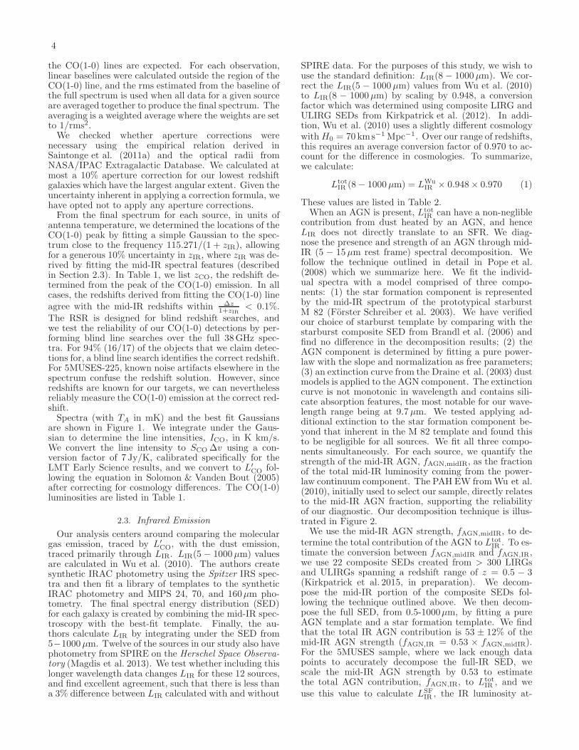
IR can have a non-negliblecontribution from dust heated by an AGN, and henceLIR does not directly translate to an SFR. We diag-nose the presence and strength of an AGN through mid-IR (5 − 15µm rest frame) spectral decomposition. Wefollow the technique outlined in detail in Pope et al.(2008) which we summarize here. We fit the individ-ual spectra with a model comprised of three compo-nents: (1) the star formation component is representedby the mid-IR spectrum of the prototypical starburstM 82 (Forster Schreiber et al. 2003). We have verifiedour choice of starburst template by comparing with thestarburst composite SED from Brandl et al. (2006) andfind no difference in the decomposition results; (2) theAGN component is determined by fitting a pure power-law with the slope and normalization as free parameters;(3) an extinction curve from the Draine et al. (2003) dustmodels is applied to the AGN component. The extinctioncurve is not monotonic in wavelength and contains sili-cate absorption features, the most notable for our wave-length range being at 9.7µm. We tested applying ad-ditional extinction to the star formation component be-yond that inherent in the M 82 template and found thisto be negligible for all sources. We fit all three compo-nents simultaneously. For each source, we quantify thestrength of the mid-IR AGN, fAGN,midIR, as the fractionof the total mid-IR luminosity coming from the power-law continuum component. The PAH EW fromWu et al.(2010), initially used to select our sample, directly relatesto the mid-IR AGN fraction, supporting the reliabilityof our diagnostic. Our decomposition technique is illus-trated in Figure 2.We use the mid-IR AGN strength, fAGN,midIR, to de-

termine the total contribution of the AGN to LtotIR . To es-

timate the conversion between fAGN,midIR and fAGN,IR,we use 22 composite SEDs created from > 300 LIRGsand ULIRGs spanning a redshift range of z = 0.5 − 3(Kirkpatrick et al. 2015, in preparation). We decom-pose the mid-IR portion of the composite SEDs fol-lowing the technique outlined above. We then decom-pose the full SED, from 0.5-1000µm, by fitting a pureAGN template and a star formation template. We findthat the total IR AGN contribution is 53 ± 12% of themid-IR AGN strength (fAGN,IR = 0.53 × fAGN,midIR).For the 5MUSES sample, where we lack enough datapoints to accurately decompose the full-IR SED, wescale the mid-IR AGN strength by 0.53 to estimatethe total AGN contribution, fAGN,IR, to Ltot

IR , and weuse this value to calculate LSF

IR , the IR luminosity at-

5

Fig. 1.— LMT/RSR spectra for our 5MUSES subsample, with antenna temperature (mK) as a function of frequency (GHz). Here weshow 14GHz of the rest frame spectra around the CO(1-0) line (this is only a portion of the full 73-111GHz observed with the RSR). Weoverplot the location of the peak of the CO(1-0) emission as the blue dotted line and the best fit Gaussian as the red dashed line for the 17sources with a 3σ detection. Seven sources lack a 3σ detection, and for those, we show an arrow at the expected location of the CO(1-0)peak emission based on zIR. The spectra are presented in order of increasing redshift.

tributed to star formation. In the analysis that follows,we separate our sources according to fAGN,midIR, result-ing in three categories: (1) purely star forming galaxieshave fAGN,midIR < 0.2 (fAGN,IR < 0.1); (2) AGN havefAGN,midIR > 0.7 (fAGN,IR > 0.4); and (3) compositeshave fAGN,midIR = 0.2− 0.7 (fAGN,IR = 0.1− 0.4).We are also interested in the strength of the PAH

emission, since this is expected to trace star formationand photodissociation regions within molecular clouds.By comparing the PAH emission with LIR and CO(1-0)emission, we have three separate tracers of the dust and

gas in the ISM which are expected to correlate with starformation. We quantify the PAH emission as L6.2, theluminosity of the isolated 6.2µm line. We fit a continuumon either side of this feature at 5.9µm and 6.5µm andremove the continuum component. We then integrateunder the continuum subtracted emission feature to ob-tain L6.2. None of our sources are extended at 8.0µmusing the Spitzer IRAC images, so aperture correctionsare not necessary when comparing the Spitzer and LMTluminosities. We list L6.2, L

SFIR , fAGN,midIR, and fAGN,IR

in Table 2.

6

Fig. 1.— (continued)

2.4. Specific Star Formation Rates

The specific star formation rate (sSFR) is the ra-tio of SFR to stellar mass. Shi et al. (2011) deter-mined stellar masses for the 5MUSES sample by fittingBruzual & Charlot (2003) population synthesis modelsto optical and near-IR broadband photometry assuminga Chabrier IMF. We adopt these stellar masses, and wecalculate the SFR from LSF

IR according to(

SFR

M⊙ yr−1

)

= 1.509× 10−10

(

LSFIR

L⊙

)

(2)

assuming a Kroupa IMF and a constant star formationrate over the past 100Myr (Murphy et al. 2011b). We

do not convert between a Chabrier IMF and a KroupaIMF for this formula, since the conversion is very small(Zahid et al. 2012).The galaxy main sequence can be used to classify

galaxies as either normal star forming galaxies or star-bursts based on whether they have an enhanced SFRfor a given M∗. This relationship is a slowly varyingfunction of redshift. Elbaz et al. (2011) present a rela-tionship between sSFR and the time since the Big Bangin Gyr, tcosmic, for the galaxy main sequence (see Equa-tion 13 in Elbaz et al. 2011). The relation in Elbaz et al.(2011) is derived assuming a Salpeter IMF, an LIR-SFRconversion from Kennicutt (1998), and a cosmology with

7

TABLE 2Infrared and Star Formation Properties

ID logLtotIR

a fAGN,midIR fAGN,IRb Typec logLSF

IRlogL6.2 logM∗ sSFRd Desig.e

(L⊙) (L⊙) (L⊙) (M⊙) (Gyr−1)

5MUSES-200 10.36 0.23 0.12 Comp 10.31 8.04 10.48 0.09 MS5MUSES-179 10.22 0.24 0.13 Comp 10.17 7.95 11.08 0.01 MS5MUSES-169 10.79 0.06 0.03 SFG 10.79 8.45 10.82 0.11 MS5MUSES-105 10.88 0.16 0.08 SFG 10.85 8.38 10.79 0.13 MS5MUSES-171 11.06 0.08 0.04 SFG 11.05 8.54 10.93 0.16 MS5MUSES-229 11.10 0.12 0.06 SFG 11.08 8.62 11.36 0.06 MS5MUSES-230 11.09 0.00 0.00 SFG 11.09 8.98 10.46 0.50 SB5MUSES-234 11.03 0.15 0.08 SFG 11.00 8.52 10.47 0.40 SB5MUSES-132 11.30 0.00 0.00 SFG 11.30 9.16 10.67 0.51 SB5MUSES-227 11.08 0.57 0.30 Comp 10.91 8.63 10.73 0.18 MS5MUSES-141 11.14 0.67 0.36 Comp 10.93 8.71 11.15 0.07 MS5MUSES-158 11.41 0.23 0.12 Comp 11.36 8.87 10.99 0.28 SB5MUSES-225 11.09 0.29 0.15 Comp 11.02 8.61 10.99 0.13 MS5MUSES-273 11.40 0.45 0.24 Comp 11.28 8.78 10.97 0.23 MS5MUSES-136 11.39 0.77 0.41 AGN 11.13 9.03 11.41 0.06 MS5MUSES-294 11.55 0.16 0.08 SFG 11.52 8.97 11.49 0.12 MS5MUSES-216 11.39 0.14 0.07 SFG 11.37 9.06 10.71 0.53 SB5MUSES-194 11.72 0.81 0.43 AGN 11.44 8.34 11.19 0.21 MS5MUSES-249 11.63 0.12 0.06 SFG 11.61 9.26 10.96 0.52 SB5MUSES-250 11.63 0.05 0.03 SFG 11.63 9.44 11.29 0.26 MS5MUSES-275 12.00 0.79 0.42 AGN 11.73 9.46 11.13 0.47 SB5MUSES-313 11.81 0.41 0.22 Comp 11.70 9.12 10.64 1.36 SB5MUSES-156 12.06 0.31 0.16 Comp 11.99 9.24 10.17 7.70 SB5MUSES-101 11.91 0.82 0.43 AGN 11.63 9.03 10.86 0.68 SB.

a The LtotIR values are scaled from Wu et al. (2010); see Section 2.3 for details.

b The fraction of LIR(8 − 1000 µm) due to heating by an AGN.c Star forming galaxies (SFG) have fAGN,midIR < 0.2 (fAGN,IR < 0.1); AGN have fAGN,midIR>0.7 (fAGN,IR >0.4); composites (Comp) have fAGN,midIR = 0.2− 0.7 (fAGN,IR = 0.1− 0.4)d Calculated using LSF

IR.

e Main Sequence (MS) or Starburst (SB) according to Equation 3, where sSFR is calculated using LSFIR .

H0 = 70 kms−1Mpc−1, Ωm = 0.3, and ΩΛ = 0.7. Weconvert the relation from a Salpeter IMF to a Kroupa

IMF using MKroupa∗ = 0.62MSalpeter

∗ (Zahid et al. 2012).We convert tcosmic to the cosmology used in this pa-per by multiplying by 1.02, appropriate for our redshiftrange. Finally, the SFRs are related by SFRMurphy11 =0.86 SFRKennicutt98 (Kennicutt & Evans 2012). Apply-ing all of these conversions gives the MS relation appro-priate for the present work:

sSFRMS (Gyr−1) = 38× t−2.2cosmic (3)

If a galaxy has a sSFR a factor of two greater thansSFRMS, it is classified as a starburst. We use zCO

and LSFIR to calculate sSFRMS and list the stellar masses

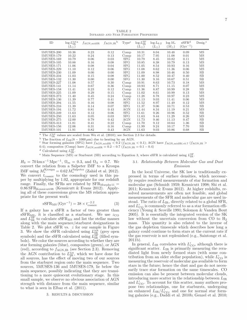
along with the main sequence/starburst designations inTable 2. We plot sSFR vs. z for our sample in Figure3. We show the sSFR calculated using Ltot

IR (grey opensymbols) and the sSFR calculated using LSF

IR (filled sym-bols). We color the sources according to whether they arestar forming galaxies (blue), composites (green), or AGN(red), according to fAGN,IR (see Section 2.3). Removingthe AGN contribution to Ltot

IR , which we have done forall sources, has the effect of moving two of our sourcesfrom the starburst region onto the main sequence. Twosources, 5MUSES-136 and 5MUSES-179, lie below themain sequence, possibly indicating that they are transi-tioning to a more quiescent evolutionary stage. In thissmall sample, we observe no obvious association of AGNstrength with distance from the main sequence, similarto what is seen in Elbaz et al. (2011).

3. RESULTS & DISCUSSION

3.1. Relationship Between Molecular Gas and DustEmission

In the local Universe, the SK law is traditionally ex-pressed in terms of surface densities, which necessar-ily require resolved measurements of star formation andmolecular gas (Schmidt 1959; Kennicutt 1998; Shi et al.2011; Kennicutt & Evans 2012). At higher redshifts, re-solved measurements are often not feasible, and globalmeasurements of the SFR and molecular gas are used in-stead. The ratio of LIR, directly related to a global SFR,and L′

CO is commonly referred to as a star formation effi-ciency (Young & Scoville 1991; Solomon & Vanden Bout2005). It is essentially the integrated version of the SKlaw without the uncertain conversion from CO to H2

mass. This quantity is also related to the inverse ofthe gas depletion timescale which describes how long agalaxy could continue to form stars at the current rate ifthe gas reservoir is not replenished (e.g., Saintonge et al.2011b).In general, LIR correlates with L′

CO, although there issignificant scatter. LIR is primarily measuring the rera-diated light from newly formed stars (with some con-tribution from an older stellar population), while L′

CO ismeasuring the reservoir of molecular gas available to formstars in the future; hence the dust and gas do not neces-sarily trace star formation on the same timescales. COemission can also be present between molecular clouds,introducing more scatter in the relationship between LIR

and L′CO. To account for this scatter, many authors pro-

pose two relationships, one for starbursts, undergoingan enhanced LIR/L

′CO, and one for normal star form-

ing galaxies (e.g., Daddi et al. 2010b; Genzel et al. 2010;

8

5

10

15

20

25

30

Flux

(m

Jy)

5MUSES-169Star Forming Galaxy

1

2

3

4

5

6

7

Flux

(m

Jy)

5MUSES-273Composite

5 6 7 8 9 10 11 12Rest Wavelength (µm)

5

10

15

Flux

(m

Jy)

5MUSES-275AGN

Fig. 2.— We determine the presence and strength of a mid-IR AGN by decomposing the mid-IR spectrum into a star for-mation component (green triple-dot-dashed line) and a power-lawcontinuum with extinction (blue dot-dashed line). We calculatefAGN,midIR as the fraction of the luminosity of the best fit model(red dashed line) due to the power-law component. We illustratethe spectral decomposition of a star forming galaxy (top panel),composite (middle panel), and AGN (bottom panel).

Carilli & Walter 2013; Tacconi et al. 2013). If a galaxyundergoes a burst of star formation that also triggersAGN growth, this could account for some of the scat-ter in LIR/L

′CO. Initially, as an embedded AGN grows

more luminous, it heats some of the surrounding dust,but is enshrouded enough that the host galaxy is stillvisible (e.g., Sanders et al. 1988; Hopkins et al. 2006;Kirkpatrick et al. 2012). The increase in the amount ofwarm dust heated by the AGN will enhance LIR but maynot yet affect L′

CO, implying an artificially high LIR/L′CO

unless the AGN contribution is accounted for (e.g., byconsidering LSF

IR ). As the AGN becomes less enshrouded,the PAH and cold dust emission from the host becomeless prominent because the dust heated by the AGN isoutshining the dust in star forming regions, and/or be-cause feedback from the AGN is quenching the star for-mation. If the AGN is quenching the star formation, thiswill produce lower LSF

IR values and hence lower LSFIR/L′

CO,unless feedback from the AGN expels CO on the sametimescales.

0.0 0.1 0.2 0.3zCO

-2.0

-1.5

-1.0

-0.5

0.0

0.5

1.0

log

sSF

R (

Gyr

-1)

Star Forming GalaxyCompositeAGNMain SequenceStarburst

Star Forming GalaxyCompositeAGNMain SequenceStarburst

0.0 0.2Fraction

Fig. 3.— sSFR vs. z for our sample. The open symbolsshow sSFR calculated with Ltot

IRwhile the filled symbols show

sSFR calculated with LSFIR . We color the sources according to

whether they are star forming galaxies (blue), composites (green),or AGN (red), according to fAGN,midIR (star forming galaxies havefAGN,midIR < 0.2; AGN have fAGN,midIR > 0.7; and compositeshave fAGN,midIR = 0.2 − 0.7). We overplot the main sequencerelation from Equation 3 (dashed line), and the grey shaded re-gion extends a factor of two above and below this line, consistentwith the scatter measured in Elbaz et al. (2011). Removing theAGN contribution has the effect of generally lowering the sSFRand moving two sources onto the main sequence. We show thedistributions of sSFRs in the histogram on the right. The greyhistogram is the distribution when sSFR is calculated with Ltot

IR ,and the cyan histogram is the distribution of sSFR calculated withLSFIR . The dashed and dot-dashed lines show the medians.

7.5 8.0 8.5 9.0 9.5 10.0 10.5 11.0log L′

CO (K km/s pc2)

10.0

10.5

11.0

11.5

12.0

12.5

log

L IRSF

(L O

•)

SFGs; Genzel et al. (2010)Starbursts; Genzel et al. (2010)Star Forming GalaxyCompositeAGNMain SequenceStarburst

SFGs; Genzel et al. (2010)Starbursts; Genzel et al. (2010)Star Forming GalaxyCompositeAGNMain SequenceStarburst

Fig. 4.— The relationship between LSFIR

and L′CO

for the5MUSES sample. We also include the relationships for LIR andL′CO derived for starbursts and star forming galaxies (SFGs) from

Genzel et al. (2010), where the grey shaded region indicates thestandard deviation. We color the points according to mid-IR powersource, and we use different symbols to indicate the galaxies thatare starbursting according to the sSFR criterion. There is nostrong separation according to either mid-IR power source or star-burstiness, and our galaxies all lie close to the SFG relation fromGenzel et al. (2010).

9

As yet, no study has attempted to quantify the effect ofthe AGN on LIR/L

′CO individually in galaxies due to the

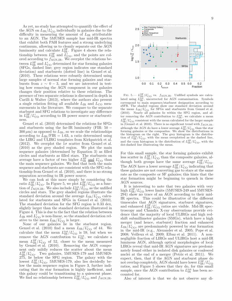
difficulty in measuring the amount of LIR attributableto an AGN. The 5MUSES sample has mid-IR spectrathat exhibit both PAH features and a strong underlyingcontinuum, allowing us to cleanly separate out the AGNluminosity and calculate LSF

IR . Figure 4 shows the rela-tionship between LSF

IR and L′CO, and the points are col-

ored according to fAGN,IR. We overplot the relations be-tween LSF

IR and L′CO determined for star forming galaxies

(SFGs, dashed line; grey region indicates one standarddeviation) and starbursts (dotted line) in Genzel et al.(2010). These relations were robustly determined usinglarge samples of normal star forming galaxies and star-bursts from z ∼ 0 − 3, and we are interested in test-ing how removing the AGN component in our galaxieschanges their position relative to these relations. Thepresence of two separate relations is discussed in depth inCarilli & Walter (2013), where the authors also presenta single relation fitting all available LIR and LCO mea-surements in the literature. We compare to the separatestarburst and SFG relations to investigate any differencein LSF

IR/L′CO according to IR power source or starbursti-

ness.Genzel et al. (2010) determined the relations for SFGs

and starbursts using the far-IR luminosity (FIR: 50 −

300µm) as opposed to LIR, so we scale the relationshipsaccording to LIR/FIR = 1.63, a ratio determined usingthe LIRG and ULIRG templates from Kirkpatrick et al.(2012). We overplot the 1σ scatter from Genzel et al.(2010) as the grey shaded region. We plot the mainsequence galaxies (determined by Equation 3) as filledcircles and starbursts as filled stars. The starbursts onaverage have a factor of two higher LSF

IR and L′CO than

the main sequence galaxies. We find that both the mainsequence and starbursts are consistent with the SFG rela-tionship from Genzel et al. (2010), and there is no strongseparation according to IR power source.We can look at this more simply by considering the

ratio LSFIR/L

′CO. In Figure 5, we plot LSF

IR/L′CO as a func-

tion of fAGN,IR. We also include LtotIR /L′

CO as the unfilledcircles and stars. The grey shaded regions illustrate thestandard deviation around the average LIR/L

′CO calcu-

lated for starbursts and SFGs in Genzel et al. (2010).The standard deviation for the SFG region is 0.33 dex,slightly larger than the standard deviation illustrated inFigure 4. This is due to the fact that the relation betweenLIR and L′

CO is non-linear, so the standard deviation rel-ative to the mean LIR/L

′CO is larger.

None of our galaxies lie in the starburst region.Genzel et al. (2010) find a mean LIR/L

′CO of 44. We

calculate that the mean LtotIR /L′

CO is 59, but when weremove the AGN contribution to Ltot

IR , we calculate amean LSF

IR/L′CO of 52, closer to the mean measured

by Genzel et al. (2010). Removing the AGN compo-nent only mildly reduces the scatter about the meanLSFIR/L

′CO. Two galaxies, 5MUSES-179 and 5MUSES-

275, lie below the SFG region. The galaxy with thelowest LSF

IR/L′CO, 5MUSES-179, also lies decidedly be-

low the main sequence region in Figure 3, further indi-cating that its star formation is highly inefficient, andthis galaxy could be transitioning to a quiescent phase.We find no relationship between LSF

IR/L′CO and fAGN,IR.

0.0 0.1 0.2 0.3 0.4 0.5fAGN,IR

1.0

1.5

2.0

2.5

log

L IRSF

/ L′ C

O

Starbursts

SFGs

Star Forming GalaxyCompositeAGNMain SequenceStarburst

Star Forming GalaxyCompositeAGNMain SequenceStarburst

0.0 0.2Fraction

Fig. 5.— LSFIR

/L′CO

vs. fAGN,IR. Unfilled symbols are calcu-

lated using LtotIR

, uncorrected for AGN contamination. Symbolscorrespond to main sequence/starburst designation according tosSFR. The shaded regions show one standard deviation aroundthe mean LIR/L′

CO for SFGs and starbursts from Genzel et al.(2010). Nearly all galaxies lie within the SFG region, and af-ter removing the AGN contribution to Ltot

IR , we calculate a mean

LSFIR /L′

CO consistent with the mean calculated for the larger samplein (Genzel et al. 2010). There is no significant trend with fAGN,IR,

although the AGN do have a lower average LSFIR

/L′CO

than the starforming galaxies or the composites. We show the distributions inthe histogram on the right. The grey histogram is the distribu-tion of Ltot

IR/L′

CO, with the mean overplotted as the dashed line,

and the cyan histogram is the distribution of LSFIR /L′

CO, with thedot-dashed line illustrating the mean.

For this small sample, the star forming galaxies exhibitless scatter in LSF

IR/L′CO than the composite galaxies, al-

though both groups have the same average LSFIR/L

′CO.

The AGN have a lower average LSFIR/L

′CO indicating that

these galaxies are not converting gas to stars at the samerate as the composite or SF galaxies; this hints that thestar formation might be beginning to quench in theseAGN sources.It is interesting to note that two galaxies with very

high LSFIR/L

′CO lower limits (5MUSES-249 and 5MUSES-

294) show no trace of an AGN according to their mid-IR spectra. This could be illustrative of the differenttimescales that AGN signatures, starburst signatures,and enhanced LSF

IR/L′CO ratios are visible. Mid-IR spec-

troscopy and Chandra X-ray observations provide evi-dence that the majority of local ULIRGs and high red-shift submillimeter galaxies (SMGs), which have a highmerger (and hence, starburst) fraction and enhancedLIR/L

′CO, are predominately powered by star formation

in the mid-IR (e.g., Alexander et al. 2005; Pope et al.2008; Veilleux et al. 2009; Elbaz et al. 2011). A non-negligible fraction of LIRGs and ULIRGs host a mid-IRluminous AGN, although optical morphologies of localLIRGs reveal that mid-IR AGN signatures are predomi-nately found either in isolated disk galaxies or coalescednuclei at the end of a merger (Petric et al. 2011). Weexpect, then, that if the AGN and starburst phase donot overlap completely, AGN should have lower LSF

IR/L′CO

ratios, and Figure 5 shows that they do, for this smallsample, once the AGN contribution to Ltot

IR has been ac-counted for.Also of interest is that we do not observe any di-

10

-3 -2 -1 0 1log sSFR

-9.5

-9.0

-8.5

-8.0

-7.5

-7.0

log

SF

R /

L′ CO

Star Forming GalaxyCompositeAGNMain SequenceStarburstSaintonge et al. (2011)Genzel et al. (2010)

Star Forming GalaxyCompositeAGNMain SequenceStarburstSaintonge et al. (2011)Genzel et al. (2010)

Fig. 6.— SFR/L′CO

/SFR, which is related to the inverse of thegas depletion timescale, as a function of sSFR. We include thelocal COLD GASS sources from Saintonge et al. (2011b) and thez = 1 − 3 sample from Genzel et al. (2010). There is a strongcorrelation between the two parameters for all galaxies, althoughthis correlation would be missed if only considering the 5MUSESsample.

chotomy in LSFIR/L′

CO either as a function of mid-IRpower source or along the main sequence/starburst clas-sification. Saintonge et al. (2011b) observe a clear re-lationship between the gas depletion timescale and thesSFR in a large, complete, sample of local galaxies aspart of the COLD GASS survey. We compare oursources with the COLD GASS galaxies in Figure 6.Saintonge et al. (2011b) calculate the depletion timescaleas tdep = MH2

/SFR, but to avoid any uncertainties dueto converting L′

CO to MH2(see Section 3.3), we simply

use the ratio SFR/L′CO ∝ t−1

dep. We have calculated the

SFRs for our galaxies using LSFIR . Figure 6 also includes

the z = 1−3 galaxies from Genzel et al. (2010), where wehave corrected the SFRs, calculated using the conversionin Kennicutt (1998), to be on the same scale as ours. TheSFRs from Saintonge et al. (2011b) are calculated by fit-ting the SED from the UV out to 70µm. We do notfurther correct for differing cosmologies as the intrinsicscatter in Figure 6 is larger than any shift introduced inthis manner.When looking at just our 5MUSES sample in Figure

6, there is no strong correlation between SFR/L′CO and

sSFR, just as we observed no separation according tosSFR in Figure 5. However, when we extend the dynam-ical range of the plot by considering the local galaxiesfrom Saintonge et al. (2011b) and the z = 1− 3 galaxiesfrom Genzel et al. (2010), there is a strong correlation(a Spearman’s rank test gives a correlation coefficient ofρ = 0.72 with a two-sided significance equal to 0.0). Oursample lies in the range expected. This suggests that weare not observing any differences between our starburstand main sequence galaxies in Figures 4 and 5 simplybecause we are not probing a large enough range of L′

COand LIR.

3.2. Comparing Different Tracers of Star FormingRegions

IR, CO, and PAH luminosities are all commonly usedas tracers of star formation in dusty galaxies. PAHemission arises from PDRs surrounding young starsand has been demonstrated locally to be largely cospa-tial with the molecular clouds traced by CO emission(Bendo et al. 2010). If star formation is continuously fu-eled for . 1Gyr, these tracers should all correlate.For most star forming galaxies, the ratio of LPAH/LIR

is fairly constant, but there is an observed deficit ofPAH emission relative to LIR in local ULIRGs, possi-bly due to an increase in the hardness of the radiationfield caused either by a major merger/starburst or anAGN (Tran et al. 2001; Desai et al. 2007). This samedeficit does not hold for similarly luminous galaxies athigh redshift, however, where the majority of ULIRGsare observed to have strong PAH emission (Pope et al.2008; Menendez-Delmestre et al. 2009; Kirkpatrick et al.2012).Pope et al. (2013) explored the evolution of L6.2/LIR

with redshift for a sample of ULIRGs from z ∼ 1 − 4as well as a sample of local ULIRGs. Specifically, theauthors compare L6.2/LIR with LIR and find that thedeficit in L6.2 relative to LIR occurs at a higher LIR

for high redshift galaxies than is seen in the local Uni-verse. Galaxies from z ∼ 1 − 3 typically have highergas fractions than local counterparts (Daddi et al. 2010a;Tacconi et al. 2010). This increase in molecular gas couldbe linked to the relative increase in PAH emission, sinceboth are largely cospatial. Indeed, when Pope et al.(2013) compare L6.2/LIR with LIR/L

′CO, they find a con-

sistent relationship for both the local and high redshiftULIRGs.We now build on the analysis presented in Pope et al.

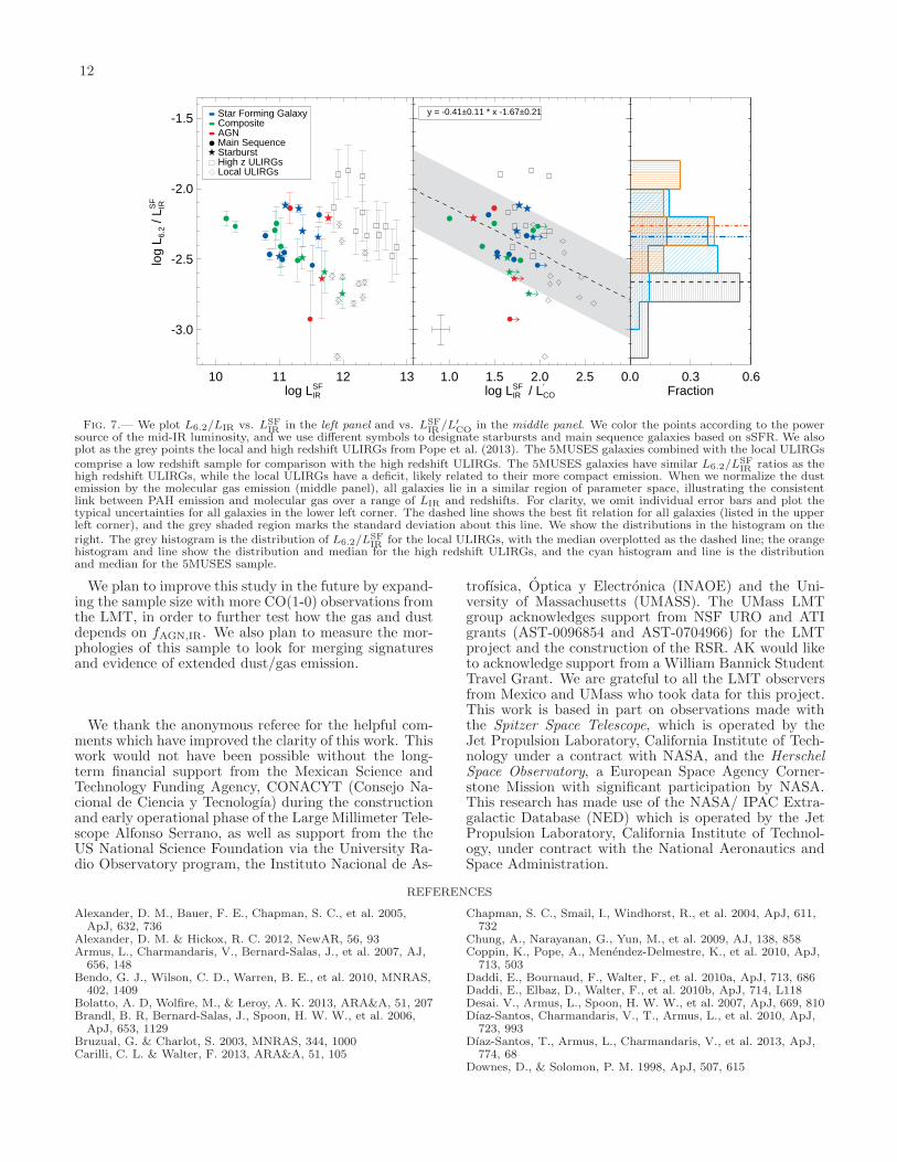
(2013) by extending the parameter space explored tothe lower luminosity 5MUSES sample. The 5MUSESgalaxies combined with the local ULIRGs comprise alow redshift sample for comparison with the high red-shift ULIRGs. We plot L6.2/L

SFIR vs. LSF

IR for our samplein the left panel of Figure 7. We also include the highredshift and local ULIRGs from Pope et al. (2013) wherewe have calculated LSF

IR for all ULIRGs by scaling themid-IR AGN strength, determined by decomposing themid-IR spectra. There is a decreasing trend between the5MUSES sample and the local ULIRGs, but the highredshift ULIRGs are shifted from this relation. In theright panel, we plot L6.2/L

SFIR vs. LSF

IR/L′CO. L′

CO iscalculated using the estimated CO(1-0) luminosity forall galaxies (see Pope et al. 2013, for conversion details).In this panel, most galaxies follow the same decreasingtrend, with a few obvious outliers. We overplot the bestfit relation for the 5MUSES sample and the local andhigh redshift ULIRGs. The shaded region indicates onestandard deviation above and below the fit. There is adecreasing correlation between L6.2/L

SFIR and LSF

IR/L′CO

for most galaxies.Figure 7 suggests that the relative amount of emission

from small dust grains is related to LSFIR/L

′CO for dusty

galaxies out to z ∼ 2. That is, weaker PAH emissionis associated with a higher star formation efficiency andfaster gas depletion timescales. The decrease in L6.2 withincreasing LIR could indicate that PAH emission in gen-eral is suppressed for more luminous galaxies. We donot find significantly lower L6.2/L

SFIR ratios for our AGN

11

or composite galaxies as compared to our star forminggalaxies, indicating that in our sample, the growing AGNis not affecting this ratio.As discussed in Pope et al. (2013), the PAH deficit

could be similar to the observed deficit in [CII] emis-sion at high LIR in local galaxies (e.g., Kaufman et al.1999; Stacey et al. 2010; Gracia-Carpio et al. 2011).Dıaz-Santos et al. (2013) probe the [CII] deficit in lo-cal LIRGs and find that galaxies with compact mid-IRemission have a [CII] deficit, regardless of the mid-IRpower source. For our sample, follow-up observationsare required to trace the compactness of the galaxies. Ifour galaxies have extended dust emission, this would ex-plain the similar L6.2/L

SFIR ratios for the 5MUSES galax-

ies and the high redshift ULIRGs, since high redshiftULIRGs are known to have extended dust emission (e.g.,Chapman et al. 2004). Based on the relative strengths ofthe dust emission and CO(1-0) emission, the 5MUSESsources, primarily LIRGs, seem to be more accuratecounterparts for the high redshift ULIRGs than the localULIRGs, evidencing the evolution of ISM properties withredshift. A morphological comparison of these sourcescould provide more insight into structure and compact-ness of the dust and gas emission.

3.3. Gas Fractions

The gas fraction is expressed as fgas = Mgas/(Mgas +M∗), where Mgas = αCOL

′CO. αCO = 4.6 is a com-

monly adopted value for normal star forming galaxies,while in starbursts, the conversion αCO = 0.8 has beenmeasured (Bolatto et al. 2013, and references therein).We have two observational indicators of starburstiness:LSFIR/L

′CO and sSFR. To calculate Mgas, we explore two

scenarios. First, we apply αCO = 4.6 to our entire sam-ple (top panel of Figure 8). None of our galaxies haveLSFIR/L

′CO indicative of a starburst (Figure 5), so apply-

ing the same αCO to the entire sample is a reasonableassumption. Second, we use αCO = 0.8 to calculate thegas mass for those galaxies with an sSFR indicative ofa starburst (bottom panel of Figure 8). We plot thegas fractions as a function of redshift We also plot gasfractions of normal star forming galaxies from the lit-erature, and we have corrected the individual αCO val-ues used to be 4.6. The average molecular gas fractionevolves with redshift, and we plot the measured relation,fgas ∝ (1 + z)2, determined from a stellar mass limitedsample with logM∗ > 10 (Geach et al. 2011), similar tothe masses of our 5MUSES sample.Our gas fractions (in both panels) lie in the range ex-

pected when comparing with the best fit line and thepoints from Leroy et al. (2009) and Geach et al. (2011).Our CO(1-0) detection rate is high (17 out of 24 sources),producing a large range of measured gas fractions. Inthe top panel, our starburst galaxies are systematicallyhigher than the main sequence galaxies, and the scatterabout the (1 + z)2 line is larger, which suggests that thelower αCO = 0.8 conversion factor might be more appro-priate for these sources if we expect similar gas fractionsfor main sequence and starburst galaxies. Theoretically,the conversion factor depends on the geometry of theCO and H2 distribution. When the CO emission is ex-tended and not confined to molecular clouds, warm, andhas a high surface density, as is the case in mergers, thenthe lower αCO value is appropriate (Bolatto et al. 2013,

and references therein). Magnelli et al. (2012) measureαCO for a sample of high redshift main sequence andstarburst galaxies and find an anti-correlation betweenαCO and sSFR, which they interpret as evidence thatthe mechanisms responsible for raising a galaxy off themain sequence must also affect the physical conditionswithin the star forming regions. We also find that the gasfractions reproduce a similar separation between sourcesas the main sequence criterion, linking αCO with thesSFR. In contrast, neither LSF

IR/L′CO nor L6.2/L

SFIR shows

any separation between the starburst and main sequencegalaxies, likely due to the limited range being probed.These ratios, then, are relatively stable for galaxies ofa limited mass and luminosity range. Narayanan et al.(2012) argue against a bimodal αCO conversion factor,and instead develop a fitting formula for the conversionfactor that depends on the metallicity and CO line in-tensity. We currently lack metallicities for our sample, sowe cannot directly apply the prescribed variable conver-sion factor. Given the continuous relationship betweensSFR and SFR/L′

CO evidenced in Figure 6, a continuous,rather than bimodal, conversion factor based on galac-tic environment may be the most appropriate choice andwould mean that all galaxies in our sample obey a simi-lar relationship between the molecular gas and the stellarmass.

4. CONCLUSIONS

We present new LMT/RSR CO(1-0) detections for 24intermediate redshift galaxies from the 5MUSES sample.We use Spitzer mid-IR spectra, available for all sources,to diagnose the presence and strength of an AGN. Weremoved the AGN contribution to Ltot

IR and probe thestar formation, gas, and dust emission using LSF

IR , L′CO,

and L6.2. We find

1. Removing the AGN contribution to LtotIR results in

a mean LSFIR/L

′CO for our entire sample consistent

with the mean LIR/L′CO derived for a large sample

of star forming galaxies from z ∼ 0 − 3. For ourfour AGN sources, removing the AGN contributionproduces a mean LSF

IR/L′CO lower than the mean

LSFIR/L

′CO for our star forming galaxies or compos-

ites. We find that LSFIR/L

′CO is not strongly cor-

related with either the sSFR or the mid-IR powersource over the range of luminosities probed.

2. The average ratio of L6.2/LSFIR in our sample is sim-

ilar to what is observed in high redshift ULIRGsrather than local ULIRGs. When we plot L6.2/L

SFIR

as a function of LSFIR/L

′CO, we find all galaxies (lo-

cal ULIRGs, our intermediate redshift 5MUSESsources, and high redshift ULIRGs) are consistentwith the same declining relationship.

3. Our starbursts have gas fractions that are clearlyoffset from the main sequence galaxies if we applya constant αCO to all galaxies which might indicatethat the two populations require different αCO val-ues. However, no dichotomy between starburstsand main sequence galaxies is evident when com-paring other quantities that probe the ISM (LSF

IR ,L′CO, or L6.2).

12

10 11 12 13log LIR

SF

-3.0

-2.5

-2.0

-1.5

log

L 6.2 /

L IRSF

Star Forming GalaxyCompositeAGNMain SequenceStarburstHigh z ULIRGsLocal ULIRGs

1.0 1.5 2.0 2.5 log LIR

SF / L′CO

y = -0.41±0.11 * x -1.67±0.21

0.0 0.3 0.6Fraction

Fig. 7.— We plot L6.2/LIR vs. LSFIR

in the left panel and vs. LSFIR

/L′CO

in the middle panel. We color the points according to the powersource of the mid-IR luminosity, and we use different symbols to designate starbursts and main sequence galaxies based on sSFR. We alsoplot as the grey points the local and high redshift ULIRGs from Pope et al. (2013). The 5MUSES galaxies combined with the local ULIRGscomprise a low redshift sample for comparison with the high redshift ULIRGs. The 5MUSES galaxies have similar L6.2/LSF

IR ratios as thehigh redshift ULIRGs, while the local ULIRGs have a deficit, likely related to their more compact emission. When we normalize the dustemission by the molecular gas emission (middle panel), all galaxies lie in a similar region of parameter space, illustrating the consistentlink between PAH emission and molecular gas over a range of LIR and redshifts. For clarity, we omit individual error bars and plot thetypical uncertainties for all galaxies in the lower left corner. The dashed line shows the best fit relation for all galaxies (listed in the upperleft corner), and the grey shaded region marks the standard deviation about this line. We show the distributions in the histogram on theright. The grey histogram is the distribution of L6.2/LSF

IRfor the local ULIRGs, with the median overplotted as the dashed line; the orange

histogram and line show the distribution and median for the high redshift ULIRGs, and the cyan histogram and line is the distributionand median for the 5MUSES sample.

We plan to improve this study in the future by expand-ing the sample size with more CO(1-0) observations fromthe LMT, in order to further test how the gas and dustdepends on fAGN,IR. We also plan to measure the mor-phologies of this sample to look for merging signaturesand evidence of extended dust/gas emission.

We thank the anonymous referee for the helpful com-ments which have improved the clarity of this work. Thiswork would not have been possible without the long-term financial support from the Mexican Science andTechnology Funding Agency, CONACYT (Consejo Na-cional de Ciencia y Tecnologıa) during the constructionand early operational phase of the Large Millimeter Tele-scope Alfonso Serrano, as well as support from the theUS National Science Foundation via the University Ra-dio Observatory program, the Instituto Nacional de As-

trofısica, Optica y Electronica (INAOE) and the Uni-versity of Massachusetts (UMASS). The UMass LMTgroup acknowledges support from NSF URO and ATIgrants (AST-0096854 and AST-0704966) for the LMTproject and the construction of the RSR. AK would liketo acknowledge support from a William Bannick StudentTravel Grant. We are grateful to all the LMT observersfrom Mexico and UMass who took data for this project.This work is based in part on observations made withthe Spitzer Space Telescope, which is operated by theJet Propulsion Laboratory, California Institute of Tech-nology under a contract with NASA, and the HerschelSpace Observatory, a European Space Agency Corner-stone Mission with significant participation by NASA.This research has made use of the NASA/ IPAC Extra-galactic Database (NED) which is operated by the JetPropulsion Laboratory, California Institute of Technol-ogy, under contract with the National Aeronautics andSpace Administration.

REFERENCES

Alexander, D. M., Bauer, F. E., Chapman, S. C., et al. 2005,ApJ, 632, 736

Alexander, D. M. & Hickox, R. C. 2012, NewAR, 56, 93Armus, L., Charmandaris, V., Bernard-Salas, J., et al. 2007, AJ,

656, 148Bendo, G. J., Wilson, C. D., Warren, B. E., et al. 2010, MNRAS,

402, 1409Bolatto, A. D, Wolfire, M., & Leroy, A. K. 2013, ARA&A, 51, 207Brandl, B. R, Bernard-Salas, J., Spoon, H. W. W., et al. 2006,

ApJ, 653, 1129Bruzual, G. & Charlot, S. 2003, MNRAS, 344, 1000Carilli, C. L. & Walter, F. 2013, ARA&A, 51, 105

Chapman, S. C., Smail, I., Windhorst, R., et al. 2004, ApJ, 611,732

Chung, A., Narayanan, G., Yun, M., et al. 2009, AJ, 138, 858Coppin, K., Pope, A., Menendez-Delmestre, K., et al. 2010, ApJ,

713, 503Daddi, E., Bournaud, F., Walter, F., et al. 2010a, ApJ, 713, 686Daddi, E., Elbaz, D., Walter, F., et al. 2010b, ApJ, 714, L118Desai. V., Armus, L., Spoon, H. W. W., et al. 2007, ApJ, 669, 810Dıaz-Santos, Charmandaris, V., T., Armus, L., et al. 2010, ApJ,

723, 993Dıaz-Santos, T., Armus, L., Charmandaris, V., et al. 2013, ApJ,

774, 68Downes, D., & Solomon, P. M. 1998, ApJ, 507, 615

13

0.1

1.0

f gas

Leroy et al. (2009)Geach et al. (2011)Tacconi et al. (2010)Daddi et al. (2010a)Geach (2011)

Leroy et al. (2009)Geach et al. (2011)Tacconi et al. (2010)Daddi et al. (2010a)Geach (2011)

Star Forming GalaxyCompositeAGNMain SequenceStarburst

Star Forming GalaxyCompositeAGNMain SequenceStarburst

0.0 0.5 1.0 1.5zCO

0.1

1.0

f gas

Fig. 8.— Gas fractions vs. zCO for our sample. Top panel: fgas iscalculated using αCO = 4.6 for all galaxies. Bottom panel: fgas iscalculated using αCO = 0.8 for starburst galaxies (filled stars). Wealso overplot gas fractions from Leroy et al. (2009), Daddi et al.(2010b), Tacconi et al. (2010), and Geach et al. (2011). The bestfit line is fgas = 0.1(1+z)2 (Geach et al. 2011). Our galaxies lie inthe region expected from the best fit line, although there is an offsetbetween the starbursts (stars) and main sequence sources (circles)when αCO = 4.6 is used, indicating that a lower αCO conversionmight be more appropriate for the starbursts.

Draine, B. T. 2003, ARA&A, 41, 241Elbaz, D., Dickinson, M., Hwang, H. S., et al. 2011, A&A, 533,

119Erickson, N., Narayanan, G., Goeller, R., Grosslein, R. 2007,

ASPC, 375, 71Evans, A. S., Frayer, D. T., Surace, J. A., Sanders, D. B. 2001,

AJ, 121, 1893Evans, A. S., Solomon, P. M., Tacconi, L. J., et al. 2006, AJ132,

2398Forster Schreiber, N. M., et al. 2003, A&A, 399, 833

Geach, J. E., Smail, I., Moran, S. M., et al. 2011, ApJ, 730, L19Genzel, R., Tacconi, L. J., Gracia-Carpio, J., et al. 2010,

MNRAS, 407, 2091Gracia-Carpio, J., et al. 2011, ApJ, 728, L7Hopkins, P. F., Hernquist, L., Cox, T. J., et al. 2006, ApJS, 163, 1Hughes, D., Jauregui Correa, J.-C., Schloerb, F. P., et al. 2010,

SPIE, 7733, 31Kaufman, M. J., Wolfire, M. G., Hollenbach, D. J., et al. 1999,

ApJ, 527, 795Kennicutt, R. C., Jr. 1998, ApJ, 498, 541Kennicutt, R., C., Jr. & Evans, N. 2012, ARA&A, 40, 531Kirkpatrick, A., Pope, A., Alexander, D. M., et al. 2012, ApJ,

759, 139Leroy, A. K., Walter, F., Bigiel, F., et al. 2009, AJ, 137, 4670Magdis, G. E., Rigopoulou, D., Helou, G., et al. 2013, A&A, 558,

136

Murphy, E. J., Chary, R.-R., Dickinson, M., et al. 2011a, ApJ,732, 126

Murphy, E. J., Condon, J. J., Schinnerer, E., et al. 2011b, ApJ,737, 67

Magnelli, G., Saintonge, A., Lutz, D., et al. 2012, A&A, 548, 22Madau, P. & Dickinson, M. 2014 ARA&A, accepted.

arXiv:1403.0007Menendez-Delmestre , K., Blain, A. W., Smail, I., et al. 2009,

ApJ699, 667Mullaney, J. R., Alexander, D. M., Goulding, A. D., Hickox, R.

C. 2011, MNRAS, 414, 1082Narayanan, D., Krumholz, M. R., Ostriker, E. C., Hernquist, L.

2012, MNRAS, 421, 3127Noeske, K. G., Weiner, B. J., Faber, S. M., et al. 2007, ApJ, 660,

L43Petric, A. O., Armus, L., Howell, J., et al. 2011, ApJ, 730, 28Pope, A., Chary, R.-R., Alexander, D. M., et al. 2008, ApJ, 675,

1171Pope, A., Wagg, J., Frayer, D., et al. 2013, ApJ, 772, 92Saintonge, A., Kauffmann, G., Kramer, C., et al. 2011a, MNRAS,

415, 32Saintonge, A., Kauffmann, G., Wang, J., et al. 2011b, MNRAS,

415, 61Sajina, A., Yan, L., Armus, L., et al. 2007, ApJ, 664, 713Sanders, D. B. & Mirabel, I. F. 1996, ARA&A, 34, 749Sanders, D. B., Soifer, B. T., Elias, J. H., et al. 1988, ApJ, 325, 74Sanders, D. B., Scoville, N. Z., Soifer, B. T. 1991, ApJ, 370, 158Schmidt M. 1959, ApJ, 129, 243Shi, Y., Helou, G., Yan, L., et al. 2011, ApJ, 733, 87Siebenmorgen, R., Krugel, E., & Spoon, H. W. W. 2004, A&A,

414, 123Solomon, P. M., & Vanden Bout, P. A. 2005, ARA&A, 43, 677Stacey, G. J., Hailey-Dunsheath, S., Ferkinhoff, C., et al. 2010,

ApJ, 724, 957Tacconi, L. J., Genzel, R., Neri, R., et al. 2010, Nature, 463, 781Tacconi, L. J., Neri, R., Genzel, R., et al. 2013, ApJ, 768, 74Tran, Q. D., Lutz, D., Genzel, R., et al. 2001, ApJ, 552, 527Veilleux, S., et al. 2009, ApJ, 701, 587Weedman, D., Charmandaris, V., & Zezas, A. 2004, ApJ, 600, 106Wu, Y., Helou, G., Armus, L., et al. 2010, ApJ, 723, 895Xia, X. Y., Gao, Y., Hao, C.-N., et al. 2012, ApJ, 750, 92Young, J. S. & Scoville, N. Z. 1991, ARA&A, 29, 581Zahid, H. J., Dima, G. I., Kewley, L. J., et al. 2012, ApJ, 757, 54