


Languages
Pages
Legal


Transient transport of polymer solution flow in porous media
Aizhan Zeinula, Bachelor in Petroleum Engineering
Submitted in fulfillment of the requirements
for the degree of Masters of Science
in Chemical Engineering
School of Engineering
Department of Chemical Engineering
Nazarbayev University
53 Kabanbay Batyr Avenue,
Astana, Kazakhstan, 010000
Supervisor: Athanasios Papathanasiou
Co-supervisor: Vasileios Inglezakis
13.12.2018

DECLARATION
I hereby, declare that this manuscript, entitled “Transient transport of polymer
solution flow in porous media”, is the result of my own work except for quotations
and citations which have been duly acknowledged.
I also declare that, to the best of my knowledge and belief, it has not been
previously or concurrently submitted, in whole or in part, for any other degree or
diploma at Nazarbayev University or any other national or international institution.
Name: Aizhan Zeinula
Date: 13.12.2018

2
Abstract
Kazakhstan takes 12th place in World oil production, however 52,7 % of
produced oil comes from “mature” fields that are on the last production stages.
Therefore, use of enhanced oil recovery methods becomes essential; one of these
methods is polymer flooding, which involves injecting a polymer solution into the
reservoir in order to displace trapped oil towards the wellbore. For successful
injection of polymer solutions in a reservoir it is essential to study properly their
behavior in porous media. This master thesis focuses on that topic, by describing
and understanding two main factors that have a great impact on polymer transport,
namely (i) the inaccessible pore volume (IPV) and (ii) polymer retention due to its
adsorption on grain surfaces within the porous medium. In order to reach this goal
experiments on core samples (plugs) were conducted, and effluent concentration
profiles were obtained. Moreover, numerical modelling was implemented to
characterize diffusion/adsorption of polymer molecules inside the porous core.
Besides characterization of the porosity of the core samples, experimental
work was based on the idea of contrasting the effluent concentration curves for
polymer solution flow with the effluent concentration curves of a tracer (sodium
chloride) during core flooding tests. The effluent concentration of tracer was
measured by an on-line resistivity apparatus, while the polymer’s concentration was

3
determined indirectly by on-line measurement of pressure drop in a long coil tube,
which was set right on the exit of the core plug. The adsorption was calculated during
polymer injection in saturated core sample and was manifested as a delay on polymer
effluent profile compared to the effluent profile of the tracer. The IPV, on other hand,
was determined during brine injection after polymer injection, and manifested as
faster polymer exit compared to the tracer; this is attributed to the multi–scale
porosity of the core material and large size of the polymeric molecules. Experimental
effluent profiles were compared to computer simulations using an in-house
developed computer code.
Our results demonstrate that adsorption of polymer molecules on grain surface
averages 0.0006 g/g, and that 14.8 % of the core plug’s pore volume is inaccessible
to the polymer solution. Also, according to mercury porosimetry, 16 % of the total
pore volume has smaller diameter than the size of the polymer molecule; this points
to a multi-scale porous structure, which is expected to affect effluent response curves.
The transport of polymer through the core was described by a multi-scale dynamic
convection/diffusion model which was implemented in-house using MATLAB. The
shapes of curves of the polymer and tracer effluent curve can be reproduced by
considering the polymer to have a higher Peclet number and lower diffisivity,
whereas the tracer species is considered to have a higher microscale diffusivity and

4
lower Peclet number. This results is consistent with the analysis of the polymer size
relative to the multi – scale porosity of the system.

5
Acknowledgments
I would like to thank Professor Athanasios D. Papathanasiou for his guidance
throughout this research and incredible support even when I stopped believing in this
work. Also my co-supervisor Professor Inglezakis for his assistance in this work and
specifically his help in the characterization of core samples using mercury
porosimetry.
I would also like to thank Dr. Adam Dobri for his invaluable help with the
modeling part. He has helped with writing the code for MATLAB software and
always was ready to give advice and feedback.
I also want to express my gratitude to Scientific Research Institute
“CaspiiMunaiGas” for supporting this project and providing with all necessary
equipment for conducting the experimental work.

6
Table of content
Abstract....................................................................................................................... 2
Acknowledgments ...................................................................................................... 5
List of Abbreviations &Symbols ............................................................................... 8
List of figures ............................................................................................................. 9
List of tables ............................................................................................................... 9
Chapter 1-Introduction ............................................................................................. 10
Chapter 1-Polymer flooding. .................................................................................... 13
2.1 The concept of polymer flooding ................................................................... 13
2.2 Worldwide experience and screening criteria for polymer flooding .............. 15
2.3 The effect of Inaccessible Pore Volume (IPV) on polymer effluent profiles 18
2.4 The effect of retention on polymer effluent profiles ...................................... 20
Chapter 3 - Methods and process of analyses. ......................................................... 23
3.1 Literature review of measuring methods of IPV and adsorption ................... 23
3.1.1. Research methods of investigation inaccessible pore volume (IPV) ........ 24
3.1.2 Research methods of investigation polymer retention ............................. 25
3.1.3 Research methods of investigation IPV and polymer retention .............. 28
3.2 Procedures to measure IPV and adsorption .................................................. 29
3.3 Polymer analysis ............................................................................................. 32
3.3.1 Determination of the physicochemical properties of the polymer ........... 32
3.3.2 Determination of the polymer solution hydrolysis degree ...................... 34
3.3.3 Measurement of the intrinsic viscosity for the calculation of the molecular
weight and molecule diameter of the polymer .................................................. 37
3.3.4 Polymer solution preparation ....................................................................... 41
3.3.5 Rheological properties of polymer ........................................................... 42
3.4 Core analyses .................................................................................................. 43
3.4.1 Core extraction ......................................................................................... 43
3.4.2 Measurement of porosity, bulk and mineralogical density of rock samples
with helium porosimeter .................................................................................... 44
3.4.3 Measurement of samples permeability on nitrogen permeameter .......... 47
3.4.4 Measuring pore size distribution using mercury porosimetry ................ 48

7
Chapter 4 Main experiment ..................................................................................... 51
4.1 System for experiment .................................................................................... 51
4.2 Data processing. .............................................................................................. 54
4.2.1 Construction of the polymer vs. concentration curve .............................. 54
4.2.2 Construction of the tracer concentration vs. conductivity curve ............. 56
Chapter 5 – Results and discussions of experimental analyses ............................... 58
5.1 Results of polymer solutions analyses ........................................................ 58
5.2 Results of core analyses .............................................................................. 61
5.3 Results of main experiments ...................................................................... 62
Chapter 6 – Comparison with numerical modelling ................................................ 67
Chapter 7 - Conclusion ............................................................................................. 76
References ................................................................................................................ 78
Appendices ............................................................................................................... 83
Appendix A ........................................................................................................... 83
Appendix B ........................................................................................................... 85
Appendix C ........................................................................................................... 97
Appendix D ......................................................................................................... 101

8
List of Abbreviations &Symbols
β Partition coefficient, defined as β= (𝐶𝑙)𝑒𝑞 (𝐶𝑏)𝑒𝑞⁄
(𝑪𝒍)𝒆𝒒 concentration in the bulk liquid at equilib- rium, mol/l
(𝑪𝒃)𝒆𝒒 concentration in the intraparticle pore volume liquid at equilibrium, mol/l
e bed voidage
EOR enhanced oil recovery
ep particle voidage
IPV inaccessible pore volume
NaCl sodium chloride
ODE Ordinary differential equations
PV pore volume
Q flow rate, m3/min
r Radius,mm
V Volume,m3
Wrock weight of rock, gr
ΔP pressure drop, psi
ΔPV incremental change in pore volume
μ dynamic viscosity, cP
μo oil phase viscosity, cP
μw water phase viscosity, cP
ν kinematic viscosity, mm2/s
ρ Density, kg/m3
ρr Resistivity, ohm
σ Conductivity, mS/m
φ Porosity, %
𝐵m Biot number, dimensionless defined as 𝐵m = keR/Deff
ke external mass transfer coefficient, cm/s
R bead radius, cm
Deff effective intraparticle diffusivity, cm*/s
𝐷r dimensionless diffusivity defined as 𝐷r =Deff/(R2(F/Vt))
F Volumetric flowrate, 1/s
Vt total reactor volume, 1
𝑃e Peclet number, dimensionless defined as 𝑃e=(uL/Dl)
u axial superficial fluid velocity in the reactor
L Reactor lenght
Dl axial dispersion coefficient, cm2/s
𝜗 Hagenbach correction factor
𝜙 Thiele Modulus, 𝜙=(R/3)(k/Deff)0.5
k First order reaction constant, cm/s

9
List of figures
Figure 1.1 Regimes of application of tertiary oil recovery methods. The circled area and the yellow
color outline the region (in terms of oil viscosity and reservoir depth) where polymer injection
might be applied. ............................................................................................................................ 11
Figure 2.1 Process of polymer flooding (Lake, 1989) ................................................................... 14 Figure 2.2 Original experimental demonstration of the inaccessible pore volume phenomenon
(concentration fraction vs volume of injected fluid/pore volume of sample) ................................ 19 Figure 2.3 Polymer retention mechanisms in porous medium ....................................................... 21 Figure 2.4 Calculated effluent profiles for a linear core system both with and without adsorption
(L(0) - linear adsorption) ................................................................................................................ 22
Figure 3.1 Rheometer - Anton Paar MCR 502 ............................................................................... 42 Figure 3.2 Soxlet apparatus for core sample’s extraction .............................................................. 43 Figure 3.3 Ultrapore 300 - helium porosimeter .............................................................................. 45
Figure 4.1 PlS-200 ......................................................................................................................... 51 Figure 4.2 AST-600 Autosaturator for sample saturation .............................................................. 52 Figure 4.3 Fluke Fluke PM 6306 for resistance measurement of effluent ..................................... 52 Figure 4. 4 Scheme of the system used in experiments ................................................................ 53 Figure 4.5 Capillary type viscometer ........................................................................................... 55 Figure 4.6 The relationship between polymer solution concentration and viscosity ..................... 56 Figure 4.7 The relationship between tracer salinity (concentration) and conductivity .................. 57
Figure 5.1 Rheological data of polymer FP3630 (log-log chart) ................................................... 59 Figure 5.2 Rheological data of polymer FP5205 (log-log chart) ................................................... 59 Figure 5.3 Rheological data of polymer FP5115 (log-log chart) ................................................... 60 Figure 5.4 The pore size distribution of core plug Akshabulak 501 .............................................. 62 Figure 5.5 Tracer effluent curve ..................................................................................................... 63 Figure 5.6 Polymer effluent curve ................................................................................................. 63 Figure 5.7 Effluent curves ............................................................................................................. 64 Figure 5.8 Calculation IPV and adsorption .................................................................................... 65 Figure 6.1 Comparing low Dr (pure dispersion case) and high Dr (diffusion in particles impacts the
response) cases ............................................................................................................................... 70 Figure 6.2 Modelling of tracer and polymer curve rise with delay ................................................ 71 Figure 6.3 Modelling of tracer and polymer curve rise without delay ........................................... 73 Figure 6.4 Modeling the polymer and tracer fall curve .................................................................. 74
List of tables
Table 3.1Table for measuring intrinsic viscosity ........................................................................... 40
Table 5.1 The physicochemical properties of polymer solution .................................................... 58 Table 5.2 Results of standard analysis of core samples ................................................................. 61 Table 5.3 Calculated IPV and adsorption foe core plug - Akshabulak 501 ................................... 65

10
Chapter 1-Introduction
“In Kazakhstan, 52.7% of produced oil is represented by mature oilfields that
have passed through the production "plateau" or are at the last stage of reservoir
production"(Bulekbai, 2013).
“More than half of the oil fields in Kazakhstan are mature, they have already
passed the peak of production and the level of production is low. Currently, the oil
recovery factor is 30%, while in the world it reaches about 50% - it is necessary to
increase it by at least 5-7%' - Bakytzhan Sagintayev, first deputy prime minister of
the Republic of Kazakhstan (Tumasheva, 2015).
Also it is a fact that a third of Kazakhstan GDP is generated by revenues from
the oil and gas industry (Statistics, 2014).
Considering this information, the importance of tertiary recovery or enhanced
oil recovery (EOR) becomes evident, as it plays a key role in the development of the
national petroleum industry.
There are many EOR techniques that can be applied and have been applied
successfully. However taking into the account that average depth of oil reservoirs in
Kazakhstan is in the range 500-2500 m (200-8000 ft) and oil viscosity may vary from
100 to 900 cP, polymer flooding (injection) according to the figure 1.1 (Anon., 2012)
could be chosen as tertiary recovery method.

11
Figure 1.1 Regimes of application of tertiary oil recovery methods. The circled area and the
yellow color outline the region (in terms of oil viscosity and reservoir depth) where polymer
injection might be applied.
Larry W. Lake (Lake, 2010) gave a comprehensive definition of polymer
flooding and how it works. Polymer flooding is a method in which a (water-soluble)
polymer powder is added to the water that is injected in reservoir, making the
resulting solution more viscous. As a result mobility ratio decreases, sweep
efficiency increases and the remaining oil is displaced towards the wellbore. These
terms will be explained in the following section.
Polymer flooding is the one the major category of chemical EOR methods
which is designed to increase required mobility ratio between polymer and oil
volume being displaced. However, the success or failure of polymer flooding is
generally affected by reservoir geology, sweep efficiency, gravity segregation etc..

12
Unfortunately we cannot directly measure the majority of the variables needed for
precise prediction of oil displacement during polymer flooding. A first step in
improving this state of affairs is to understand the behavior of polymer solutions in
a laboratory environment, specifically their flow behavior in porous core samples,
obtained from the reservoir of interest. There are two main components that affect
the polymer behavior in a porous medium, namely (i) polymer retention and (ii)
inaccessible pore volume (IPV) (Idahosa, 2016). Polymer retention consist of
mechanical entrapment, adsorption and hydrodynamic retention, while inaccessible
pore volume refers to the inability of large polymer molecules to flow through small
pore spaces. These parameters are determined through measurement of effluents'
(polymer and tracer) profiles in one-dimensional core injection experiments. The
data collected in such laboratory experiments are vital for further modelling of this
EOR process (Ferreira et al, 2016).
In this study provides one-dimensional (1-D) core flooding experiments were
performed, using polymer solution (hydrolyzed polyacrylamide) and tracers (sodium
chloride), in order to better understand the transport behavior of the polymer
molecules.
13
Chapter 1-Polymer flooding.
2.1 The concept of polymer flooding
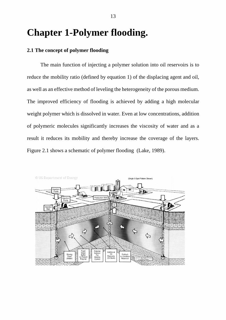
The main function of injecting a polymer solution into oil reservoirs is to
reduce the mobility ratio (defined by equation 1) of the displacing agent and oil,
as well as an effective method of leveling the heterogeneity of the porous medium.
The improved efficiency of flooding is achieved by adding a high molecular
weight polymer which is dissolved in water. Even at low concentrations, addition
of polymeric molecules significantly increases the viscosity of water and as a
result it reduces its mobility and thereby increase the coverage of the layers.
Figure 2.1 shows a schematic of polymer flooding (Lake, 1989).

14
In case where the viscosity of oil considerably exceeds the viscosity of the
forcing-out agent (water) it is necessary to increase the viscosity of the pumped
water and reduce its mobility; a direct consequence of this is that the minimum
amount of water is used and also, that the maximum quantity of oil is recovered.
Use of excess water leads to a significant reduction in final oil recovery (water
uselessly circulates through the washed zones, and the oil stays in reservoir) and
also to large economic losses associated with water pumping, recycling and
transportation.
The Mobility Ratio (M) is determined as the ratio of the mobility of the
injectant fluid (water or polymer solution) to the mobility of the displaced fluid
(oil). The mobility ratio is a dimensionless number and an indicator of efficiency
of displacemant:
𝑀 =𝜆𝑤
𝜆𝑜=
𝑘𝑤µ𝑤
⁄
𝑘𝑜µ𝑜
⁄, (1.1)
Where
𝜆𝑤- water mobility, mD/cP;
Figure 2.1 Process of polymer flooding (Lake, 1989)

15
𝜆0-oil mobility, mD/cP;
𝑘𝑤 , 𝑘0- relative permeability of water and oil respectively, mD;
µ𝑤 , µ𝑜- viscosity of water and oil respectively, cP;
For successful oil displacement, the Mobility Ratio (M) has to be less than
1. Otherwise, it was lead to viscous fingering effect i.e. water flows through
washed zones, oil remains in the reservoir, and this will result in excess water
production (watercut) (Don W. Green, 1998). One of the method to increase the
mobility ratio is to adding chemicals in order to increase the water viscosity – thus
the method of polymer flooding.
2.2 Worldwide experience and screening criteria for polymer flooding
The polymer flooding method in the world is studied since the end of the
1950s, and in industrial conditions is tested since the 1960s. Commercial
experiments and also use of polymers in industrial volumes for the purpose of
increasing oil production in various geological conditions were conducted on
numerous locations worldwide: USA, Canada, China, France, India, Indonesia,
Venezuela, Germany, Brazil, Argentina (Delamaide, 31 March-2 April 2014) . In
recent years the world leader in the field of polymer flooding is China - projects
on polymer flooding are implemented from the 1990s. Twenty-five years'
successful experience of application of polymer flooding in China has shown that
it can effectively be applied on fields with watercut higher than 95%, providing
increase in oil recovery to 10% (Wang, 2008) (Chang, 2006) (Appendix A ).

16
Polymer flooding is successfully applied on the large-scale Daqing oil field of
China. This field is characterized by a complex geological structure and high
heterogeneity of collectors. Reservoir oil average viscosity is 9 MPa.s, water is
low-mineralized, and the reservoir temperature 113 °C. The PetroChina company
since 1994 has carried out six pilot projects in layers with various collector
(sandstone and conglomerate). The average increase in oil recovery in
comparison with water flooding was 15 – 20% (Wang, 2008).
In Kazakhstan the first experience of polymer flooding was carried out on
the field Kalamkas in 1981. This field’s oil is heavy, highly-resinous, sulphurous,
with viscosity up to 25 MPa.s in reservoir conditions. To prepare the polymer
solution the Albian/Cenomanian water from specially drilled wells was a source
for trial flooding. On the chemical composition Albian/Cenomanian water
belongs to chlor-calcicitic type with the salinity 93 g/l, and density 1,07 g/cc.
Originally in 1981 - 1983 the efficiency of polymer flooding was low due to high
salinity and composition of the injected waters. In 1983-1986 in this field
injection of viscoelastic structures has led to decrease in watercut from 1,5% to
0,2% a month. By 1990 the oil recovery was 33% at water content of 56%. At
usual flooding such oil recovery can be reached at 98% watercut (98% of
produced fluid is water) (Киинов, 1994) (Надиров Н. К., 1982).
The analysis of worldwide experience of this technology shows that
polymer flooding can be conducted in fields with wide variety of geological
properties. (Appendix A). Polymer flooding was used in the fields layered by

17
sands, sandstones and conglomerates, including clay sandstones. Successful
application of polymer flooding has also been reported in limestone reservoirs,
however, at the same time big losses of polymer due to adsorption are observed.
Therefore the collector type in principle isn't the limited factor however from the
economic reasons the terrigenous type of a collector is more favorable.
The fields’ depth fluctuates within 579-2205 m. This parameter isn't
limiting, however polymer flooding isn't recommended to be used in layers
located as at very high and very low depths. In the layers located at a low depth,
limiting factor is the injecting pressure which can approach the hydraulic
fracturing pressure. In layers located at a higher depth the method is not
recommended mainly because of high reservoir temperatures and the salinity of
waters (Lake, 1989) (Taber, 1997).
The effective thickness of layers varies between 3-38 m, and average
porosity in the range of 7-32%, in this regard these parameters aren't defining.
One of the most important parameter is the average permeability of reservoir and
its variability. When injecting solution of polymer in reservoirs with low
permeability two problems can arrise: a decrease in well production and an
increase in degradation of polymer solution due to high injection pressure. The
lower limit of permeability is defined around 200 mD. In layers with high
permeability increased concentration of polymer are required and this affects the
economics of the process (Abou-Kassem, 1999) (J.J. Taber, August 1997).

18
The reservoir temperature should be varied from 33 to 77 ° C. At higher
temperatures, thermal degradation of polymer can occur.
Analyzing the data presented in Appendix A (worldwide experience of
polymer floodimg), it is obvious that desirable to use low-mineralized water to
prepare the polymer solution, and where the reservoirs have highly mineralized
water, fresh water buffer need to be injected to protect the polymer solution. For
the first time this approach was implemented at the North Burbank field in 1970
(P.D. Moffitt, 1993) (Joseph C. Trantham, 1982).
Analysis of world experience shows that the maximum efficiency from the
use of polymer flooding technology gives an oil increase 5-10% (Lake, 1989).
2.3 The effect of Inaccessible Pore Volume (IPV) on polymer effluent profiles
The term "Inaccessible Pore Volume" (IPV) was originally introduced by
R. Dawson and R.B. Lantz in 1972. They found that not all open pore spaces can
contribute to polymer flow and that pore spaces inaccecible to polymer molecules
are filled with water resulting in polymer concentration changes (Dawson &
Lantz, 1972). They related this phenomena to the differing size of pore spaces,
some of which are too small for polymer’s molecule to flow through them.
Therefore the term IPV is associated with the velocity enhancement of polymer
solution comparing to tracer, as polymer’s molecule avoid small pore spaces and
only flow through the macro-scale pores. In the experiments that were conducted
by K.S. Sorbie (K.S. Sorbie,1991) larger velocity enhancement were observed for
larger polymer's molecular size and in the cores with low permeability; IPV factor

19
do not depend from concentration or flow rate. However this statement a quite
controversial, as Gupta and Trushenski (Gupta, 1978) reported that with some
change in the concentration, velocity enhancement changes too, but later Lotsch
(Lotsch, et al., 1985) did not noticed such change in his study. Stavland (
Stavland, 2010)presented the following equation to calculate IPV:
𝐼𝑃𝑉 = 1 − √1
1+𝐵 , (2.1)
where B is a dimensionless constant, calculated as kw/kp (ratio of water to oil
permeabilities of the core sample)
However all the sources related to inaccessible pore volume underline that
the inaccessible pore volume takes place when there is no adsorption (discussed
later).
On the effluent profile, the presence of Inaccessible Pore Volume is
demonstrated as followes (Dawson & Lantz, 1972):
Figure 2.2 Original experimental demonstration of the inaccessible pore volume
phenomenon (concentration fraction vs volume of injected fluid/pore volume of sample)

20
In the figure 2.2 is seen that the polymer flows faster than the tracer in a
porous medium. Polymer is just too large to fit the small pore sizes therefore
polymer just flow over it instead of flowing through pores. The tracer here helps
to identify the inaccessible pore volume effect. Pancharoen, et al. concludes in his
study that interpretation of IPVis best achieved with effluent profile comparing to
the breakthrough curve (Pancharoen, et al., 2010).
2.4 The effect of retention on polymer effluent profiles
Retention has a great impact to the polymer flow in porous media as it
includes to the adsorption, mechanical entrapment and hydrodynamic retention
(Ferreira et al, 2016). Adsorption has the biggest effect on retention, which is
considered an irreversible process. According to the D.G. Hatzignatiou, U. L.
Norris and A. Stavland polymer retention is primarily caused by its adsorption on
rock surfaces (Hatzignatiou, et al., 2013). D. Wang recommends choosing the size
and molecular weight of polymer to be small enough in order for it to easily flow
through porous media without clogging the pore space and mechanical trapping
(Wang, et al., 2008). Moving to the mechanical entrapment and hydrodynamic
retention, they are considered as reversible processes, controlled by changing the
flow condition (Ferreira et al, 2016). A good way of illustrating this phenomena
was found in the research of (Aluhwal, 2008) (figure2.3)
According to Sorbie & Phill the hydrodynamic retention is the least well
studied mechanism of polymer retention, also there is the lack of comprehensive
definition that will explain this process. (Sorbie & Phill, 1991). However Zhang

21
& Seright fully described this mechanism in their experimental study. They
explained this kind of retention as a retention occurring due to hydrodynamic
forces (Zhang & Seright, 2015). According to their laboratory data, it was proven
that the hydrodynamic retention is directly affected by flow rate. Moreover,
almost all hydrodynamic retention was irreversible, what is confirmed by
unchangeable residual resistance factor (ratio of water mobility before and after
polymer injection). However this study concluded that the enhanced oil recovery
rheology is dominated more by intrinsic property (intrinsic viscosity, molecular
eight and polymer’s molecule size) than by retention. So they contradict the
proposal of Chauveteau that rheology is primary related to retention (Chauveteau,
et al., 2002).
Figure 2.3 Polymer retention mechanisms in porous medium
Adsorption on other hand is physically present in porous media, and could
dramatically decrease rock’s permeability (Seright, et al., 2010). In the laboratory
experiments on core flooding this phenomenon is manifested as a dramatic

22
increase in the pressure gradient when core is post-flushed with water in contrast
to the water preflush. On the effluent profile adsorption is shown as delay
comparing to the no adsorption (figure 2.4). Here is assumed the Langmuir form
of the adsorption
Figure 2.4 Calculated effluent profiles for a linear core system both with and without
adsorption (L(0) - linear adsorption)
23
Chapter 3 - Methods and process of
analyses.
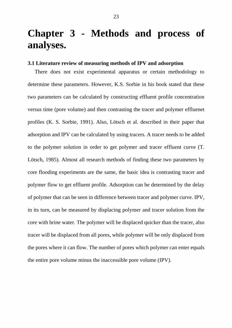
3.1 Literature review of measuring methods of IPV and adsorption
There does not exist experimental apparatus or certain methodology to
determine these parameters. However, K.S. Sorbie in his book stated that these
two parameters can be calculated by constructing effluent profile concentration
versus time (pore volume) and then contrasting the tracer and polymer effluenet
profiles (K. S. Sorbie, 1991). Also, Lötsch et al. described in their paper that
adsorption and IPV can be calculated by using tracers. A tracer needs to be added
to the polymer solution in order to get polymer and tracer effluent curve (T.
Lötsch, 1985). Almost all research methods of finding these two parameters by
core flooding experiments are the same, the basic idea is contrasting tracer and
polymer flow to get effluent profile. Adsorption can be determined by the delay
of polymer that can be seen in difference between tracer and polymer curve. IPV,
in its turn, can be measured by displacing polymer and tracer solution from the
core with brine water. The polymer will be displaced quicker than the tracer, also
tracer will be displaced from all pores, while polymer will be only displaced from
the pores where it can flow. The number of pores which polymer can enter equals
the entire pore volume minus the inaccessible pore volume (IPV).

24
3.1.1. Research methods of investigation inaccessible pore volume (IPV)
The first researcher who has reported the IPV term was Dawson and Lantz in
1977. They defined the inaccessible pore volume as the space which polymer’s
molecules hop, so the molecules of polymer are too large to fit in the pore space.
(Dawson & Lantz, 1972) After they published their paper, many researchers have
confirmed that by comparing polymer and tracer flow, concluding that polymer
flows through porous media faster than tracer, when there is no adsorption due to
inaccessible pore volume for polymer. (Dawson & Lantz, 1972; G. Paul Willhite,
1977; Chauveteau, 1982).
Stavland in his laboratory experiments measured IPV based on the difference
between water and polymer solution permeability. So, the polymer solution was
injected at different flow rates and the apparent viscosity was measured by
stabilized pressure drop. He concluded that the apparent viscosity was less than
the bulk viscosity at low shear rates, and this could be explained by the assumption
that at low shear rates polymer does not enter the entire pore volume. Even though
the IPV can be calculated, there is no methods to estimate the adsorption. (A.
Stavland, 2010).
M. Pancharoen conducted experiment that proved that statement. To measure
the IPV during core flood, the adsorption, first, was minimized by saturating the
core with the 2000 ppm polymer solution until it reached equilibrium. Then the
polymer was mixed with inorganic salt – NaCl and injected to core, after that the
effluent was collected and separated into salt and polymer in order to measure

25
their concentration. The polymer concentration was determined by using a
Ultraviolet–visible spectrophotometer (Lambda 35, Perkin-Elmer), while the
concentration of salt were identified by titration with silver nitrate (AgNO3).
Finally, to calculate IPV the difference between breakthrough curve of polymer
and salt was used. And it was clearly seen from the experiment that polymer flows
faster through core material if there is no adoption or it is minimized (M.
Pancharoen, 2010).
3.1.2 Research methods of investigation polymer retention
C. Huh (C. Huh, 1990) used sodium bromide as a tracer to investigate polymer
retention in porous media. The polymer solution with tracer was injected in a core
plug with residual oil saturation at a constant rate until the effluent concentration
stabilized. Then, polymer injection was followed by water injection to estimate
the irreversible retention of the polymer from a mass balance. Effluent samples
were collected and analyzed to measure polymer concentration by an HPLC
method with a refractive index detector and concentration of tracer using ion
chromatography. The work concludes that polymer retention increases with
increase in polymer concentration and flow velocity.
D. Broseta in his laboratory measurements of polymer retention used
potassium iodide (KI) as a tracer. He conducted the core flooding experiments
under residual oil saturation conditions and 100% brine saturated core without
any oil, also he tested the adsorption in hydrophilic and hydrophobic rocks. The
adsorption/retention was calculated by the delay of polymer in effluent profile

26
(concentration vs pore volume) The concentration of the tracer was detected by
UV spectroscopy, while the concentration of the polymer was measured using the
Dohrmann carbon analyzer. Also, it was concluded that hydrophobic cores have
stronger adsorption than hydrophilic, but in oil residual conditions the adsorption
increases in hydrophilic cores due to additional adsorbing oil surface. (Daniel
Broseta, 1995) The same tracer was used by R.N. Manichand in 2014. An in-line
spectrophotometer, with wavelength detection 230 nm was used to detect tracer –
KI and also polymer. However, unlike the previous experiment, the polymer
concentration was calculated by the polymer viscosity that was measured using a
small-diameter capillary tube that was set up on the exit of core holder with
accurate digital pressure transducer. (R.N. Manichand, 2014). Using the pressure
drop across the capillary tube, length and diameter of the tube and recording the
time that polymer is needed to flow through the tube, viscosity was calculated
using Poiseuille’s equation (Womersley, 1955).
The classical tracer/polymer methods were conducted to measure polymer
retention by J. E. Juri et al. However instead of using classical capillary
viscometer, innovative inline viscometer was set at the effluent stream at
anaerobic conditions. This allowed to avoid the problems of chemical degradation
due to the reaction with oxygen. The effluent concentration was determined by
COD (Chemical Oxygen Demand) and bleach method. They concluded that the
extended injection and backflow test obtained accurate results on retention,

27
degradation, pressures and rates behaviors with no adjustable parameters (Juri, et
al., 2015).
Unlike other researchers D.G. Hatzignatiou et.al experimentally investigated
polymer flow in water and oil–wet core samples. Instead of using tracer in the
polymer retention investigation, they connect capillary tube to core holder and
measure pressure drop along the core holder and this capillary tube. Retained
polymer volume was calculated based on the residual water saturation and the
polymer breakthrough that is determined using plot of pressure drop across the
core and the capillary tube. So, the injected polymer breakthrough occurs when
the capillary pressure drop is equal to the average value of the pressure drop
before and after breakthrough. Also, it needs to be noted that the average pressure
is associated with a 50% concentration of a polymer solution. In their paper, they
concluded that wettability has great impact on the polymer retention, indicating
that oil-wet formation has the very low amount of retention comparing to the
water–wet. This phenomenon is explained by the assumption that oil covers the
boundaries of the rock grains, thus preventing polymer molecules to interact with
them (Hatzignatiou, et al., 2013).
Wan investigated how oxygen presence impacts on polymer retention. In his
paper, he measured the polymer retention by static (mixing with loose sand) and
dynamic methods (core floods). Also, the experiments were conducted in
conditions with presence of oxygen (aerobic), and with no atmospheric or
dissolved oxygen (anaerobic). Potassium iodide (KI) was used as a tracer and

28
dissolved in polymer solution. It was underlined that from static retention
measurements there is a little difference between aerobically or anaerobically
conditions, while from the dynamic retention measurements there is too high
polymer retention in aerobic condition which is explained by chemical
degradation of polymer in presence of oxygen (Wan & Seright, 2016).
3.1.3 Research methods of investigation IPV and polymer retention
A detailed description about measuring of IPV and adsorption was given by
Lötsch et al. In their research, they used inorganic salts as a tracer and to
distinguish between the tracer and polymer they set up the densitometer and
capillary viscometer in the exit (T. Lötsch, 1985). The adsorption has nonlinear
relation to the concentration, when it is the reversible, so the adsorption could be
described by a Langmuir or a Freundlich isotherm (Moore, 1963)
K.S. Sorbie, in other hand, used radioactive chlorine-36-beta - labelled brine.
Polymer concentration were measured by a modified phenol-sulfuric acid method
with an auto analyzer and the levels of beta radio- activity were determined with
a Beckman TM scintillation counter. (K.S. Sorbie, 1987)
W.T. Osterloh and E.J. Law in their polymer transport experiments used salts
as a tracer. They conducted four step injection experiment:
1. Injection of polymer and tracer until the effluent concentration is equal to
the initial polymer concentration

29
2. Injection of brine until the effluent concentration of polymer and tracer is
too low to measure
3. Repetition of step1
4. Repetition of step2
The polymer adsorption/retention was calculated by comparing the polymer
effluent concentration in steps 1 and 3, the IPV was calculated by comparing the
tracer and polymer effluent curves in step 3. The in-situ viscosity was calculated
by measuring the pressure drop across core holder at various concentrations and
rates. (Osterloh & Law, 1988)
E.S. Moe in his work investigate the IPV and polymer retention by ordinary
tracer/polymer method. As a tracer was used inorganic salt, and the concentration
of tracer was used based on its resistivity. The polymer concentration, on the other
hand was calculated by measuring the viscosity of the polymer flowing through
the coil that was set up on the exit of core holder. After constructing the effluent
profile the IPV and retention was calculated by determining the area under
effluent curves (Moe, 2015).
3.2 Procedures to measure IPV and adsorption
To meet master thesis objectives the methods of used in research Eline Moe
(Moe, 2015) was chosen because the accurate concentration of tracer can be
estimated through resistivity, based on the salt solution conductivity, and the

30
polymer concentration could be measured without contact with oxygen, so, the
chemical degradation may be excluded .
The effluent profile is find by the following steps:
1. Prepare polymer solution with tracer in it
2. Inject the solution through core plug until pressure stabilization
3. Displace polymer solution with water until pressure stabilization
During the first injection of polymer solution with tracer (salt water) the tracer
will come out first, and then the polymer solution, due to the adsorption of
polymer solution on core’s rock surface. During the second injection with water
the polymer solution will be replaced faster than tracer due to inaccessible pore
volume for polymer. The effluent curve is constructed based on the concentrations
of the polymer solution and tracer and pore volume. Thus the adsorption is found
by taking the integral between the tracer and polymer effluent curve during the
injection of mixed solution through core plug. And the IPV is calculated by taking
integral between polymer and tracer effluent curve during displacing with water.
The concentrations of the 2 curves (polymer and tracer) should be normalized
to take the integrals by the following equation:
𝐶𝑛𝑜𝑟𝑚 =𝐶−𝐶𝑚𝑖𝑛
𝐶𝑚𝑎𝑥−𝐶𝑚𝑖𝑛, (3.1)
Where
C- concentration of fluid at the effluent
𝐶𝑚𝑖𝑛 - minimum concentration of fluid

31
𝐶𝑚ax maximum concentration of fluid
The IPV is calculated by taking the integral over time (or number of pore
volumes) of the difference between the normalized tracer concentration and
normalized polymer concentration. The unit pore volumes, PV is the time divided
by the amount of the time that it takes for one pore volume’s worth of fluid to
flow through the sample. The equation for IPV is
IPV = ∫(𝐶𝑡𝑟.𝑛𝑜𝑟𝑚 − 𝐶𝑝𝑜𝑙.𝑛𝑜𝑟𝑚)dPV , (3.2)
where
𝐶𝑡𝑟.𝑛𝑜𝑟𝑚-normilized tracer concentration
𝐶𝑝𝑜𝑙.𝑛𝑜𝑟𝑚-normilized polymer concentration
PV- pore volume.
As the time – measurement (and therefore the number of pore volumes) is
discrete, the integral is evaluated by the trapezoidal approximation.
The equation for the adsorption is
𝐴𝑑𝑠𝑜𝑟𝑝𝑡𝑖𝑜𝑛 = {∑[(𝐶𝑡𝑟.𝑛𝑜𝑟𝑚 − 𝐶𝑝𝑜𝑙.𝑛𝑜𝑟𝑚) ∗ 𝛥𝑃𝑉] + 𝐼𝑃𝑉}∗ 𝑃𝑉 ∗ 𝐶𝑝𝑜𝑙,𝑚𝑎𝑥/𝑊 𝑟𝑜𝑐𝑘,
(3.3)
where
PV is the pore volume of the rock,

32
Wrock is the weight of the rock.
3.3 Polymer analysis
Analyses for 3 different polymers was conducted in order to choose one of them.
The polymers were provided by the French company SNF. These polymers are
used on the Kazakhstan’s oil fields:
FP 3630
FP 5115
FP 5205
3.3.1 Determination of the physicochemical properties of the polymer
The method is based on the calculation of the non-volatile content
substances in powdered polymers by loss in weight after drying. The purpose of
measuring this method is to determine polymer content in polymer powder to
prepare solution with accurate concentration.
Equipment, reagents and materials:
- Weighing bottles;
- Analytical balance with weighing accuracy 0.0001 g;
- Desiccator
- Drying or heating cabinet (T = 105 ± 2 ° C).

33
Weighing bottles washed with chrome mixture, and after washed 2-3 times with
distilled water. The washed weighing bottles are dried in a drying cabinet at 105
± 2 ° C to a constant weight. Dried weighing bottles are stored in a desiccator.
A pre-dried to constant weight and weighted portion of the polymer is
placed in the weighing bottles, then it is evenly distributed on the bottom of the
weighing bottles. The weighing bottles is capped and weighed. The result is
recorded in grams accurate to the fourth decimal place.
The open weighing bottles with the sample is placed in a drying cabinet and
dried at a temperature of 105 ± 2 ° C to constant weight (weight change not more
than 0.0005 g). After drying, the bottles are cooled in a desiccator to room
temperature and weighed. The first weighing is carried out after 2 hours of drying,
the next after 0.5 hours. The degree of rounding weighing results is 0.0001g.
The polymer content is calculated as a percentage using the equation:
𝑊 =𝑚1−𝑚2
𝑚100 % (3.4)
Where
m1 – mass of weighing bottles before drying, gr;
m2 – mass of weighing bottles with polymer powder before drying, gr;
m – mass of polymer powder, gr;.

34
3.3.2 Determination of the polymer solution hydrolysis degree
The method is based on direct titration of the carboxyl groups of the
acrylamide polymer in aqueous solution with alkali. There is a relation between
molecular weight and hydrolysis degree, the higher the molecular weight the
higher the hydrolysis degree. High molecular weight results in larger moleculas
size (described later), and results in high IPV effect. However high hydrolysis
results in low adsorbtion, as the negative carboxyl groups are repulces from
negatively charged core samples’ particle surface (F.D. Martin, 1975). Thus, the
hydrolysis degree is one of the parameter to choose the optimum polymer solution
that will be used in experimental work.
Equipment, reagents and materials:
- Analytical balance with weighing accuracy 0.0001 g;
- paddle stirrer for highly viscous media;
- Titration installation in accordance;
- Magnetic stirrer;
- pH meter with a measurement error of 0.05;
- Glass cylinder;
- Glass cup;
- Burettes;
- 0.1 molar solution of HCl;
- 0.05 molar solution of NaOH;
- Distilled water according.

35
For the analysis polymer solution with a concentration of 0.05-0.1% in
distilled water is used. A portion of the polymer is calculated taking into account
the mass fraction of the main substance by the equation:
𝑚 =𝐶∗𝑃
𝑊, (3.5)
Where
С – polymer concentration in solution, %;
Р – polymer solution mass, gr;
W – polymer content (activity of polymer solution), %.
The calculated mass of the polymer is weighed on an analytical balance
with an accuracy of the third decimal place. Distilled water is poured into the
beaker in the volume required for the analysis, minus the weight of the polymer
sample. A glass of water is placed under the paddle stirrer and the stirring is turned
on; the speed of mixing should ensure the creation of a funnel. The polymer is
putted evenly among the funnel. The polymer solution is dissolved until complete
homogenization, dissolution evaluation is carried out visually by the absence of
polymer globules and solution uniformity. For analysis, the 200 cm3 of polymer
solution is took, then pH is measured and up to value to pH = 3.8 with
hydrochloric acid. Then titration is carried out with sodium hydroxide solution to
pH 7.5. The volume of NaOH solution, used to titration of the polymer solution
is measured. At the same time the control measurement with the same volume of

36
distilled water is performed with the same operations as with the working sample
of the polymer. The degree of hydrolysis of the polymer in percent is calculated
by the following equation:
𝛼 =(𝑉−𝑉𝑜)∗𝐶∗𝑀∗10−3
𝑚−(𝑉−𝑉𝑜)∗𝐶∗23∗10−3 , (3.6)
where
V and Vo – volume of NaOH solution spent on working and blank sample
titration, ml;
m – the weight of the polymer sample contained in the solution taken for
titration, g;
C - exact molar concentration of the NaOH solution, mol / l;
M - molar mass of acrylamide, g / mol;
23 - molecular weight of sodium, g / mol;
10-3 - conversion factor from cm3 to dm3
As a result of the analysis is taken the arithmetic average of two parallel
measurements, the difference between them should not exceed 0.5%. The results
were rounded up to 0.1%.
If a polymer manufacturer provides a technical documentation with different
methods for determining degree of hydrolysis, then whole analysis is performed
in accordance with the manufacturer's documentation.

37
3.3.3 Measurement of the intrinsic viscosity for the calculation of the
molecular weight and molecule diameter of the polymer
This method is based on measurement of time taken for a solution of dilute
polymer and sodium chloride to flow through a capillary viscometer of a certain
diameter. By measuring the intrinsic viscosity the molecular weight can be
calculated, and by calculating the molecular weight diameter of polymer
molecules can be identified. By knowing the molecules’ size and pore size
distribution, the rough assumption about fitting the polymer molecules in pore
size may be done. The result is obtained by using the procedure for viscosity
measurement of polymer solutions with different concentrations and by
extrapolating the experimental data to zero concentration in accordance with the
Huggins equation:
η = [η]+KC[η]2 , (3.7)
where
ηrv - reduced viscosity, dL / g;
[η] - intrinsic viscosity, dL / g;
C - polymer concentration, g / dL;
K - the Huggins constant.
Equipment, reagents and materials:
- Analytical balance with weighing accuracy of 0.0001 g;
- Blade mixer with adjustable rotation speed;

38
- Ubbelohde viscometer with a capillary diameter 0.54 or 0.84 mm;
- Mechanical stopwatch with 0.2 s. scale;
- Cylinder;
- Pipette 1.2-2-20 and pipette 1.2-2-5.10;
- Glass;
- Pear rubber;
- Thermostat suitable for glass viscometers, that maintains the temperature of 25
± 0.1 ° C;
- Sodium chloride, pure and filtered solution with a mass fraction of 10%,;
- Distilled water according;
- Acetone;
- Chrome mix.
Before making measurements on the viscometer, a portion of a polymer
with mass of 1.5-3.0 g. is weighed (the result is recorded in grams up to the fourth
decimal place) and evenly added with stirring to a solution of sodium chloride
with a volume of 100 cm3. The mixture is stirred in a blade mixer until the solution
is completely homogenized. In addition, dissolution rate should be visually
checked every 15 minutes by pouring the solution from one glass to another.
The mass concentration (C) of the obtained polymer solution is calculated
by the equation:
𝐶 =𝑚∗𝑊
𝑉∗100, (3.8)
where

39
m - the mass of the polymer sample, g;
W - the mass fraction of the main substance in the polymer,%;
V - the volume of sodium chloride taken to dissolve the polymer, dL.
Before taking measurements, the viscometer is washed with a chromium
mixture, rinsed with distilled water, acetone, and dried. 20 cm3 of the filtered
polymer solution is placed into the Ubbelohde viscometer by pipette, then whole
viscometer is moved into thermostat for 10-15 minutes at a temperature of 25 °
C. At the same time, it is necessary to ensure that the capillary and the viscometer
ball are completely immersed in a thermostatic liquid. The polymer solution is
sucked into the viscometer ball just above the top mark by using a rubber bulb
with a tube assembled on the knee of the viscometer. Furthermore, the second
knee of the viscometer should be closed using clamp on a rubber tube assembled
at the end of the knee. Then the clamp is slightly opened and at the moment when
the polymer solution passes the upper mark, stopwatch starts tracking time for
polymer solution to flow from the upper mark of the measuring ball to the lower
mark. This test is carried out at least three times and then the average value of
three parallel measurements is calculated. After that, the polymer solution is
diluted in the viscometer itself by consistently adding 4.0 cm3 of sodium chloride
solution thoroughly mixed with a pear. Then whole viscometer is thermostated
again, and after each dilution time taken for polymer solution to drain is
determined.

40
The mass concentration of dilute polymer solutions (Ci) is calculated by the
equation:
𝐶𝑖 =𝑚∗𝑉
𝑉𝑝, (3.9)
Where
C - the initial mass concentration of the polymer solution, g / dL;
V - initial volume of the polymer solution, cm3;
Vp - volume of the diluted polymer solution, cm3.
At least five dilutions should be made considering that the correct limiting
viscosity number measurement, the solutions concentration in the viscometer
should be limited to the area where the relative viscosity lies in the range 2.0 -
1.2. Sodium chloride solution used for dilution should be thermostatted in the
same thermostat. By the end of the test, the viscometer should be accurately
washed, dried, and then 20 cm3 of sodium chloride solution is poured and the time
for the solvent to drain is measured by the above method. Measurement and
calculation data are entered in table 3.1.
Table 3.1Table for measuring intrinsic viscosity
Measurements V1 V2 V3 V4 V5
Polymer drainage time , sec. (t) t1 t2 t3 t4 t5
Solvent drainage time, sec. (t0) t0 t0 t0 t0 t0
Relative viscosity ηrel=t/ t0 ηrel1 ηrel2 ηrel3 ηrel4 ηrel5
Specific viscosity ηsp = ηrel -1 ηsp1 ηsp2 ηsp3 ηsp4 ηsp5
Mass concentration of polymer solution,
g/dL Ci
C1 C2 C3 C4 C5
Reduced viscosity, dL/g ηsp/ Ci ηsp1/ C1 ηsp2/ C2 ηsp3/ C3 ηsp4/ C4 ηsp5/ C5

41
Data is processed by graphical method concentration C versus reduced
viscosity ηsp/ Ci. Through the data points straight line is constructed until
intersection with y-axis. The intersection point equals to the intrinsic viscosity.
To calculate the molecular weight the following following equation of is used
(Flory, 1953):
[η]=K’*Ma , (3.10)
Where
M – is molecular weight
K’, a are empirical constants for the system polymer – solvent
The diameter of polymer molecule in μm is found by the equation (Flory, 1953):
dp=8(M*[η])1/3 , (3.11)
3.3.4 Polymer solution preparation
Considering the established concentration of polymer solution, calculation
for determination of quantity of the dry polymer powder required for preparation
the necessary amount of polymer solution is calculated by a equation:
𝑊𝑝𝑟 =𝑊𝑠∗𝐶𝑠∗10−4
𝐴𝑝𝑟 , (3.12)
Where
𝑊𝑝𝑟- weight of dry polymer powder, g
𝑊𝑠 – weight of polymer solution, g
𝐶𝑠 – polymer solution concentration, ppm
𝐴𝑝𝑟 – activity of polymer solution, % (90-95 %).

42
The amount of the necessary water required for preparation of necessary
volume of polymer solution is determined by the equation (8).
𝑊𝑏𝑠 = 𝑊𝑠 − 𝑊𝑝𝑟 , (3.13)
where:
𝑊𝑏𝑠 – weight of water for preparing polymer solution, g.
After determination of necessary parameters (Wpr, Wbs), using the glass, the
magnetic stirrer and water, polymer solution was prepared. The preparation time
is approximately 2-3 hrs. The polymer solution with concentration 2000 ppm was
prepared.
3.3.5 Rheological properties of polymer
Rheological characteristics of polymers was determined on the rheometer - Anton
Paar MCR 502 at the room temperature and shear speeds from 1 to 100 with-1.
Processing of results were conducted by software of RHEOPLUS/32 V3.62. By
results of test dependences of dynamic viscosity on shear speed are constructed.
Figure 3.1 Rheometer - Anton Paar MCR 502

43
3.4 Core analyses
Core analyses on 6 different samples was conducted in order to choose one.
3.4.1 Core extraction
For core material analysis, determination of their various properties, it is
necessary to have a pure sample of this rock, devoid of all fluids saturating it. In
this regard, the ready samples after obtaining the correct shape of the cylinder and
symbols have been sent for extraction.
The extraction means the process of sample pore space cleaning from oil,
bitumen, water and salts. The samples extraction in our case was carried out on
Soxhlet. Prior to extraction, the plugs have been weighed on an analytical balance
with accuracy to 0.001 g.
Figure 3.2 Soxlet apparatus for core sample’s extraction

44
The samples cleaning have been carried out Soxhlet apparatus with
washing by organic solvents. As the solvent, the alcohol-benzol mixtures have
been used. The principle of Soxhlet apparatus operation is very simple. The
solvent vapors enter through a side tube in the extractor, and then in a refrigerator,
are condensed and liquid thus formed fills the container, where the sample are,
which are in the extractor. When the fluid in the extractor reaches the knee of the
outlet tube (siphon), it flows back into the flask, and wherein the solvent boils.
During the cleaning process, the samples have been tested for luminescence
under UV light. In conjunction with the solvent color, this procedure has been
used to determine the indicator of cleaning from hydrocarbons (HC). After full
cleaning, all samples at temperature of 1050С have been dried in the drying oven
(DKN 600) to the constant weight.
3.4.2 Measurement of porosity, bulk and mineralogical density of rock
samples with helium porosimeter
In order to measure the reservoir porosity and permeability, the computer
station “Abacus” of automated data input by weight and size of the sample have
been used. The results of samples weighing on an analytical balance with
accuracy to 0.001g, and the average value of sample size determined by means of
digital caliper ruler (length and diameter is measured up to 10 times)
automatically have been filled in a specially created table.

45
Figure 3.3 Ultrapore 300 - helium porosimeter
After obtaining the basic parameters of weight and volume, the samples
have been placed in the glass desiccator in order to reduce the adsorption of
atmospheric moisture and transferred to further conventional analysis
(determination of porosity and gas permeability).
In order to measure the volume of samples grain the calibrated helium
porosimeter (ULTRA-PORE 300) have been used operating on the principle of
Boyle's Law (3.14).
𝑃1 ∙ 𝑉1 = 𝑃2 ∙ 𝑉2, (3.14)
The equation used to calculate the grains volume is derived from the basic
equation of Boyle's law as follows:
𝑃1 ∙ 𝑉𝑅𝑒𝑓 = 𝑃2 ∙ (𝑉𝑅𝑒𝑓 + 𝑉matrix − 𝑉Grains), (3.15)
where:
𝑃1 - pressure in comparison chamber;
𝑉𝑅𝑒𝑓 - volume of comparison chamber, cm3;
𝑃2- pressure after helium diffusion in core glass;
𝑉𝑚𝑎𝑡𝑟𝑖𝑥- volume of core glass, cm3;

46
𝑉𝑔𝑟𝑎𝑖𝑛𝑠- volume of sample grain, cm3.
Further porosity (3.16), bulk density (3.17) and mineralogical density
(3.18) of rock sample have been calculated using the equation below:
𝜑 =(𝐿∙𝜋∙
𝐷2
4)−𝑉Grains
(𝐿∙𝜋∙𝐷2
4)
∙ 100, (3.16)
𝜌volume =𝑚sample
(𝐿∙𝜋∙𝐷2
4), (3.17)
𝜌miner =𝑚sample
𝑉Grains , (3.18)
where:
𝜑 – sample porosity, %;
𝐿– sample length, cm;
𝐷 – sample diameter, cm;
𝜌𝑣𝑜𝑙𝑢𝑚𝑒 – bulk density of sample, g/cm3;
𝜌𝑚𝑖𝑛𝑒𝑟 – mineralogical density of sample (grain density), g/cm3;
𝑚𝑠𝑎𝑚𝑝𝑙𝑒 – dry weight of sample, gr.
It should be noted that determined porosity is meant as open porosity and
accordingly, the mineralogical density of rock has an apparent mineralogical
density, if closed porosity is present in the analyzed sample. Bulk density is the
ratio of mass of core plug to the bulk volume, while grain density is the density
of rock - forming minerals.

47
3.4.3 Measurement of samples permeability on nitrogen permeameter
Measurement of the absolute permeability of samples has been carried out
using gas (nitrogen) on the calibrated equipment ULTRA-PERM 600 equipped
with new mass flow meters and pressure sensors. The software makes the
calculations using Darcy and Klinkenberg equations to calculate the gas
permeability and reciprocal of average pressure.
Figure 3.1 ULTRA-PERM 600 - Nitrogen permeameter
The Darcy equation as applied to compressible gasses is used by the
software to calculate the gas permeability. This has the following form:
𝐾𝑔 =1000∙𝑃1∙𝜇∙𝑄1∙𝐿
(𝑃12−𝑃2
2)∙𝐴, (3.19)
where:
𝐾𝑔 – gas permeability, mD;
𝜇– gas viscosity, cP;
𝑄1 - gas flow value, cm3\sec;
𝑃1– input pressure, atm;
𝑃2– downward pressure, atm;

48
𝐴– section area of sample perpendicular, cm2;
𝐿– sample length, cm.
3.4.4 Measuring pore size distribution using mercury porosimetry
In this method, at each pressure step the saturation of pore space with
mercury is estimated by determining the amount of mercury remaining in the
penetrometer tube. As the pressure increases, mercury penetrates into the pore
structure from the tube. The volume of mercury in the penetrometer is measured
by determining the electrical capacity of the penetrometer. Mercury porosimetry
(POREMASTER 60) is based on the capillary principle, which causes the
penetration of liquid into small pores. This principle is expressed by Young-
Laplace equation (3.20):
𝑃𝑐 = (1
𝑅1+
1
𝑅2), (3.20)
where
Pc – capillary pressure, kPа;
– surface tension, kPa/cm;
R – radii of curvature, cm
For cylindrical porous tube model, the two radiuses of curvatures are
similar, and the Young-Laplace equation (3.20) becomes:
𝑃𝑐 =2
𝑅, (3.21)

49
The relationship between the radius of curvature and the radius of a capillary tube
is:
→ , (3.22)
By replacing (3.22) for (3.21), Young-Laplace equation for cylindrical porous
tube model:
, (3.23)
where
Pc – capillary pressure, kPа;
– surface tension, kPa/cm;
– contact angle, °;
R – radius of curvature, cm
The capillary pressure is related to the mercury injection pressure:
Pc=Pmercury-Pair , (3.24)
Since the test starts with a vacuum, Pair≈ 0, equation (3.25) will be:
𝑃𝑐 = 𝑃𝑚𝑒𝑟𝑐𝑢𝑟𝑦 =2𝑚𝑒𝑟𝑐𝑢𝑟𝑦−𝑎𝑖𝑟∗𝑐𝑜𝑠
𝑟𝑖 , (3.25)
By solving equation (3.25) for ri, the pore size:
, (3.26)
where,
R
rcos
r
cos
R
1
rPк
cos2
ртути
iP
r cos2
Pmercury

50
ri – pore radius in sample, mkm;
σ – surface tension between mercury and air, kPa/cc;
– contact angle, °;
Pmercury –mercury injenction pressure, MPа.
The effect of surface tension between mercury and air is expressed through the
contact angle:
, (3.27)
The total volume of mercury in the penetrometer at the transition from the
low-pressure to the high-pressure is given by the equation:
𝑉𝑚𝑒𝑟𝑐𝑢𝑟𝑦 =Δw
ρ𝑚𝑒𝑟𝑐𝑢𝑟𝑦, (3.28)
Where
Δw – difference in the weight of sample,
ρmercury – density of mercury, g/cc.
The total amount of mercury in the penetrometer is expressed by the
following:
Vmercury = Vpen-Vs → Vs=Vpen-Vmercury , (3.29)
where,
Vpen – volume of penetrometer, ml;
Vmercury –volume of mercury in penetrometer measured before going from
the low-pressure to the high-pressure, ml.
Vs – total volume of sample, ml.
ртутиртути
iPP
r43161,90130cos4852
145038,0
Pmercur
y
Pmercur
y

51
The following conversion values were applied for calculations:
Parameter
System
«gas-
mercury»
«gas-reservoir
brine» «gas-oil»
«oil-
reservoir
brine»
Mercury contact angle 130
Mercury IFT 485
Labouratory contact angle 0 0 30
Labouratory IFT 70 24 35
Contact angle of the collector 0 30
IFT of the collector 50 25
Labouratory TcosTheta 70 24 30,3
Collector TcosTheta 50 21,7
IFT – Inverse Fourier Transformation, IFT * cosin of contact angle: 311,8
The results of 6 samples are presented in Appendix B
Chapter 4 Main experiment 4.1 System for experiment
For carrying out tracer experiments on core plugs, the PLS-200 system
(figure 4.1) with 4 hydrostatic coreholders was used. Samples were initially
saturated with salt water – 100 g/l NaCl, and then plugs were inserted in
hydrostatic coreholders.
Figure 4.1 PlS-200

52
For sample saturation with salt water, an automatic saturator (AST-600)
(Figure 4.2) was used, which allows to choose in the automated order time of
pumping of air and pressure of saturation for fast and full saturation of samples
of a core.
For water and polymer injection two-cylinder piston pumps and cylindrical
container with piston replacement were used, so the accurate flow rate may be
controlled.
At the effluent of the core holder steel coil with length 4.14 m and diameter
0.89 mm was established, the pressure gradient inside the coil was measured in
order to calculate the concentration of polymer solution at the effluent.
After the coil to measure resistance of the effluent Fluke apparatus (figure
4.3) was set in order to calculate the concentration
of the tracer. A diagram of the core flooding
experimental set up is shown on the Figure 4.4.
Figure 4.3 Fluke Fluke PM 6306 for resistance
measurement of effluent
Figure 4.2 AST-600
Autosaturator for sample
saturation

53
Figure 4.4 Scheme of the system used in experiments
1) Pump
2) Flask with polymer solution and tracer (150 g/l NaCl)
3) Cylindrical container with salt water (100 g/l NaCl)
4) Core holder
5) Core plugs
6) Steel coil
7) Pressure transducer
8) PC
9) Fluke resistance apparatus
10) Flask
11) Three – way valve
The procedures of conducting experiment:
1. 100% saturated with 100 g/l NaCl core plug were inserted in core holders
and closed hermetically

54
2. Polymer solution with tracer (150 g/l NaCl) in cylindrical container -3 were
pumped form down to core holder with flow rate 2 ml/min
3. The effluent goes through the coil first, pressure gradient measured and sent
to computer
4. After the coil the effluent goes through resistance apparatus, the data were
collected via wed-camera
5. After pressure and resistance stabilization the pump was switched to the
salt water (100 g/l NaCl) in order to find IPV.
6. The step 4 and 5 repeated.
4.2 Data processing.
4.2.1 Construction of the polymer vs. concentration curve
To construct polymer curve concentration versus time, pressure gradient in
coil was recalculated to the viscosity by the using Hagen-Poiseuille equation:
μ =ΔPπ𝑟4
8𝐿𝑄 , (4.1)
where
ΔP- pressure gradient through coil
r-radus of the coil tube (0.445 mm)
L – length of the coil tube (4.14 m)
Q- flow rate of liquids. (2 ml/min)

55
To find the concentration of polymer through measurement of viscosity during
the experiment the relationship between concentration and viscosity must be
determined. For this purpose the viscosity of polymer solutions at different
concentrations was measured with capillary viscometer. (Figure 4.5)
The polymer solution is filled in tube 2 until it reaches the line 8. Then the
time of flowing solution between mark 5 and mark 7 is recorded. These steps
repeated 3 times for accurate result.
Knowing the calibration constant for each viscometer (K) the kinematic
viscosity is found by equation (4.2)
v=K*(t-𝜗), (4.2)
Where
t- time, sec
𝜗 - the Hagenbach correction factor. 𝜗 = 0 when t <
400 sec
The dynamic viscosity is calculated by equation 4.3.
μ = 𝜌 ∗ v, (4.3)
The relationship between polymer solution
concentration and viscosity is shown on the figure 4.6
Figure 4.5 Capillary
type viscometer

56
Figure 4.6 The relationship between polymer solution concentration and viscosity
The relationship can be expressed by equation 4.4
y = 0.0041x + 0.7735, (4.4)
So the polymer concentration is found by equation 4.5
Cpol= (μ-0.7735)/0.0041, (4.5)
4.2.2 Construction of the tracer concentration vs. conductivity curve
Tracer curve was constructed based on the relationship between salt water
conductivity and concentration. The core was initially saturated with 100 g/l
NaCl, while the tracer concentration was 150 g/l NaCl, and the concentration of
displaced water was 100 g/l NaCl.
The conductivity (𝜎) of water was calculated through the measured resistivity (𝜌)
𝜎=1/𝜌, (4.6)
The relationship between tracer salinity (concentration) and conductivity is
shown on the figure 4.7.

57
Figure 4.7 The relationship between tracer salinity (concentration) and conductivity
Thus, the tracer concentration can be calculated by the equation 4.7.
Ct=( 𝜎-72.062)/0.7141, (4.7)

58
Chapter 5 – Results and discussions of
experimental analyses 5.1 Results of polymer solutions analyses
Three polymer powder was analized before conducting experimental work.
The polymer content, hydrolysis degree, molecular weight, diameter of polymer
molecules and rheological properties was identified. The raw data and calculated
values are presented in Appendix C.
Table 5.1 The physicochemical properties of polymer solution
Polymer
content
(activity of
polymer
solution),
%
Hydrolysis
degree, %
Intrinsic
viscosity,
dl/g
Molecular
weight,
g/mol *106
Diameter of
polymer
molecule,
μm
FP 3630 90.27 25 19.452 10.07 0.474
FP 5205 90.36 15 17.613 9.90 0.447
FP 5115 90.6 11 16.790 9.61 0.435

59
Figure 5.1 Rheological data of polymer FP3630 (log-log chart)
Figure 5.2 Rheological data of polymer FP5205 (log-log chart)

60
Figure 5.3 Rheological data of polymer FP5115 (log-log chart)
The polymer FP 5205 was chosen to conduct the main experiment as it has
optimal properties: average molecular weight and average diameter of polymer’s
molecule. If the polymer FP 3630 would be chosen the adsorbtion and IPV value
will be to high due to high molecular weight and as result large molecules, even
if it has the highest hydrolysis degree. And if the polymer FP 5115 would be
chosen there is a possibility that due to small molecules the IPV effect would not
be measured.
From the rheology results it is noticed that for the lowest concentration – 500
ppm of all 3 polymer solutions, the curves are instable. This phenomena may be
described by the idea that there can be some errors by measuring low viscosity
solutions by rheometer Anton Paar MCR502.

61
5.2 Results of core analyses
Table 5.2 Results of standard analysis of core samples
N
o
Name of
sample
Sam
pli
ng
dep
th, m
Dry
wei
gh
t o
f sa
mp
le, g
Vo
lum
e o
f p
lug
, cm
3
Len
gth
of
sam
ple
, cm
Dia
met
er o
f sa
mp
le,
cm
Vo
lum
e o
f sa
mp
le g
rain
, cm
3
Po
re v
olu
me,
cm
3
Po
rosi
ty,
%
Bu
lk d
ensi
ty o
f ro
ck, g
/cm
3
Min
eral
og
ical
den
sity
of
rock
, g
/cm
3
Gas
per
mea
bil
ity
, m
D
1 Akkudyk 20 2253.2
4 41.65
21.5
1
3.1
8
2.9
3
15.8
0
5.7
1
26.
6
1.9
4
2.6
4 687.6
2 Akkudyk 19 1920.3
4 41.28
21.3
0
3.1
9
2.9
2
15.6
7
5.6
4
26.
5
1.9
4
2.6
3 552.4
3 Botakhan 1705.4 43.11 21.8
1
3.1
9
2.9
5
16.3
4
5.4
7
25.
1
1.9
8
2.6
4
604
4 Akshabulak 45 1777.3 40.7 21.5 3.1
7
2.9
4
15.3
4
6.1
5
28.
6
1.8
9
2.6
5 321.80
5 Akshabulak
206
1883.3
7 43.6 21.6
3.1
8
2.9
4
16.5
4
5.0
2
23.
3
2.0
2
2.6
3 891.10
6 Akshabulak
501
1656.5
9
106.8
8
50.0
2
4.5
0
3.7
6
40.3
1
9.7
1
19.
4
2.1
4
2.6
5
1210.0
0
After measuring the total porosity, permeability and pore size distribution,
it was decided to use core plug #6. As it has the highest gas permeability -1210
mD, even the porosity is not highest, the pore size distribution, comparing to
others is quite good, 62.3%of pores are belong to the pores from 1 to 50 μm.
(Figure 5.1). Other core plugs’ pore size distributions are presented in Appendix
B.

62
Figure 5.4 The pore size distribution of core plug Akshabulak 501
5.3 Results of main experiments
The plots of tracer and polymer curves are shown in figure 5.5 and 5.6
respectively. The pore volume at the x-axis is equal to the multiplication of flow
rate to the total time and divided by pore volume of core plug, which is equal to
the 9.71 cm3 (Table 5.2).

63
Figure 5.5 Tracer effluent curve
Figure 5.6 Polymer effluent curve
The normalized concentration of each curve is presented on figure 5.7. The
normilized concentration was calculated according to equation 3.1.

64
Figure 5.7 Effluent curves
The adsorption and IPV values were calculated according to equations 3.2
and 3.3. (Table 5.3) To determine the integral between the tracer and the polymer
curve while the polymer injection and integral between the tracer and the polymer
curve during the water injection after the polymer injection the MATLAB
software was used. (Figure 5.8). The code is shown in Appendix D.

65
Figure 5.8 Calculation IPV and adsorption
Table 5.3 Calculated IPV and adsorption for core plug - Akshabulak 501
Value
Weight of sample, g 106.88
Volume of sample, cc 50.02
Pore volume of sample, cc 9.71
Total porosity of sample, % 19.4
IPV 14.8
Adsorption, g/g 0.0006
Polymer adsorbed, g 0.064
According to the conducted research it should be mentioned that the
concentration of effluent polymer is not equal to the concentration of injected
polymer. If the concentration of injected polymer was 2000 ppm, the maximum

66
concentration of effluent was around 1500 ppm. This phenomenon may be
explained by the fact of the mechanical destruction during polymer flow through
porous media and permanent trapping of the larger molecules of polymer between
the core’s grains. Also, the concentration of polymer curve at the beginning and
the end of the experiment reached values close to zero, but did not go down to
zero. This fact can be most likely due to sensitivity of pressure transducers, as the
tracer viscosity is very low it is very problematic to record pressure gradient inside
the coil tube. The same behavior was noticed in tracer curve, which can be
explained by the dissolving of salts from core’s grains.
Another interesting conclusion is the fact that IPV is 14.8%, while
according to the pore size distribution the percentage of pores that was smaller
than the diameter of polymer is 16%. Even if these numbers are not equal they are
pretty close and the difference can be attributed to the polydispersity of the actal
polymer solution. Additionally, the difference between these two numbers may
be due to a discrepancy between the measured pore size distribution and the pore
size distribution in the actual core, as for the former measurement (mercury
porosimetry) a small part of core was taken.

67
Chapter 6 – Comparison with numerical
modelling
To help understand the phenomena happening during polymer solution flow
through core sample, a multi-scale model was implemented in MATLAB. The
code was written based on the scientific paper of Papathanasiou et al - “Dynamic
Modeling of mass transfer phenomena with chemical reaction in immobilized-
enzyme bioreactors” (Papathanasiou, 1988). Although the paper is for the fluid
bed immobilized – enzyme bioreactors, it includes the important parameters to
describe the behavior of polymer solution in porous media containing multi-scale
porosity. These are mass transfer and diffusion characteristics, as well as a first-
order intraparticle chemical reaction. The model considers the following factors:
mass accumulation and consumption in intrapracticle space
mass diffusion into the pore spaces
Uniformity of species activity all over particles
stationary particles
The model is used to take into account diffusion/reaction inside the small
grains (or within the microscale porosity) that are described using ordinary
equations which can be easily solved in MATLAB. The diffusion of a species
within the grains (bead) is impacted by a combination of these factors, in
dimensionless form, typical values are given in square brackets:

68
𝐷R - dimensionless diffusivity, to describe how accessible the reactant is
diffuse to the particles [10-4 to 50]
β – Partition coefficient to describe the partitioning of a substance between
the bulk and the intrapracticle space
𝐵m -Biot number, describes how effectively the reactant travels from the
solution to the particles [0.01 to 100]
𝑃e - Peclet number, ratio of the superficial fluid velocity and the reactor
length to the axial dispersion
e- bed voidage, ratio of empty space to total volume of the column
ep – particle voidage, ratio of empty space to volume of the bead
𝜙 -Thiele Modulus, a measure of how fast the reaction occurs [0 to 10].
In accordance with dispersion model presented in the paper the mass balance
in the bulk liquid (dimensionless) is:
𝜕𝐶𝐿
𝜕𝑡𝑅= (
1
𝑃𝑒) (
𝜕2𝐶𝐿
𝜕𝑥2) − (
𝜕𝐶𝐿
𝜕𝑥) − 𝑄∗, (6.1 )
where
𝐶𝐿- concentration in the bulk liquid
𝑄∗ - fluid to particle mas flux, 𝑄∗ = 3 (1 − 휀)[𝐷𝑒𝑓𝑓
𝑅(𝐹
𝑉𝑇)] (
𝜕𝐶𝑅
𝜕𝑟) r=R
𝑡𝑅 = dimensionless time, 𝑡
𝜀(
𝐹
𝑉𝑇)
𝑃𝑒 = Peclet number, dimensionless, 𝑢𝐿/𝐷𝐿
𝑥 = dimensionless axial distance

69
The relation between the concentration at the particle surface (CR) and the
concentration in the bulk liquid (CL) is determined by the method outlined in the
publication. After discretization of Equation (6.1 ) into N nodes, the set of ODEs
for node “i” are given by the following equations where n = 1, 2 … n0.
𝜕𝐶𝑖
𝜕𝑡𝑅= [(
1
𝑃𝑒𝛿𝑥2+
1
2𝛿𝑥) 𝐶𝑗−1 − (
2
𝑃𝑒𝛿𝑥2+ 3(1 − 휀)𝐵𝑚𝐷𝑅) 𝐶𝑖
+ ((3(1 − 휀)𝐵𝑚𝐷𝑅))β𝐶𝑅𝑖 +휀𝐷𝑅
𝑆𝑖 𝐶𝑗+1] , (6.2 )
𝑑𝐶𝑅𝑖
𝑑𝑡𝑅=
𝐵𝑚
2휀𝑝
휀𝐷𝑅
𝑆𝑖𝐶𝑖 −
휀𝐷𝑅𝛽
𝑆𝑖(
9𝜙2𝑆𝑖
𝛽+
𝐵𝑚
2휀𝑝) 𝐶𝑅𝑖 −
휀𝐷𝑅
𝑆𝑖∑ Ψ𝑖
𝑛
𝑛𝑜
1
, (6.3 )
𝑑Ψ𝑖𝑛
𝑑𝑡𝑅= [
𝐵𝑚
2휀𝑝
휀𝐷𝑅
𝑆𝑖𝐶𝑖 −
휀𝐷𝑅𝛽
𝑆𝑖(
9𝜙2𝑆𝑖
𝛽+
𝐵𝑚
2휀𝑝) 𝐶𝑅𝑖 −
휀𝐷𝑅
𝑆𝑖∑ Ψ𝑖
𝑛
𝑛𝑜
1
+ 9휀𝐷𝑅𝜙2𝐶𝑅𝑖 − (9휀𝐷𝑅𝜙2 + 휀𝐷𝑅𝜋2𝑛2)Ψ𝑖𝑛] , (6.4 )
The resulting system of N(2+n0) ODEs can be solved using standard ODE
solvers in MATLAB.
Based on the dynamic model, figure 6. 1 shows how varying the diffusivity

70
values affect to the concentration profile of the effluent. Case 1 has a Dr=0.0001
– low enough that the species does not diffuse within the particles of the
immobilized bed. The rapid increase in concentration is explained by the fact that
molecules hop between small spaces between particles since, due to its larger
molecule size it cannot diffuse into the micro-porous space, and therefore
spreading takes short time. Case 2 (Dr=50), on other hand, corresponds to
molecules which easilty diffuse into the micro-porous space (in our case, smaller
molecules) , and as a result we observea slower increase in effluenet
concentration. In this case, polymer molecules have to travel through the entire,
micro- and macro-porous space before exiting the sample.
Figure 6.1 Comparing low Dr (pure dispersion case) and high Dr (diffusion in particles
impacts the response) cases

71
Case n N Dr Bm β 𝜙 Pe e ep delay
1 25 100 0.001 1 1 0 3 0.3 0.7 0
2 25 100 10 1 1 0 3 0.3 0.7 0
To compare the predicted response to the experimental data, two 2
different regimes were studied: the rise (polymer injection) and fall (brine
injection). Thus we can use modelling to helping explain what is happening
during the core experiments: polymer and brine injection.
Figure 6.2 Modelling of tracer and polymer curve rise with delay
Case n N Dr Bm β 𝜙 Pe e ep delay
1 25 100 0.7 1 1 0.3 10 0.7 0.9 650
2 25 100 100 1 1 0 5 0.7 0.9 0
The parameters for tracer and polymer rising curve are compared in figure
6.2. The delay of polymer curve takes place due adsorption to the grain. The

72
adsorption of the polymer solution is characterized by the capture of the polymer
by small pores (dynamic adsorption) and the deposition of the polymer on a solid
pore surfaces (static adsorption). We can assume that these phenomena can be
approximated by a first order reaction between polymer solution and particles and
take φ = 0.3 (a good fit with experimental data was obtained using this value). As
it is noticed from figure 6.2 polymer species corresponds to the lower diffusion
(fit with low Dr and high Pe values), whereas the tracer to a higher amount of
diffusion (fit with high Dr and low Pe values). The diffusion of polymer in porous
media is governed by the heterogeneity of the core sample, especially by multi-
scale porosity. The diffusion for polymer species is associated with inaccessible
pore volume effects that accelerate the polymer solution through a permeable
medium. The relation between Peclet number and diffusion is indicated by the
fact that low Peclet number corresponds to large values of diffusivity whereas
high Peclet number – smaller values of diffusivity (Kirby, 2010).
In our case, the fast molecular diffusion of the tracer can be explained by the fact
that tracer accessibly flows through core plugs due to its small molecule size.
Polymer agent, in other hand, is not accessible to the particles due to the IPV
effect, and therefore the diffusivity is low.

73
Figure 6.3 Modelling of tracer and polymer curve rise without delay
Case n N Dr Bm β 𝜙 Pe e ep delay
1 25 100 10 0.1 0.2 0 3 0.4 0.2 0
2 25 100 4 1 0.15 0 500 0.4 0.2 0
Figure 6.3 represents the same experimental data of polymer and tracer rise
but with another set of parameters. As it seen from the figures (6.2 and 6.3) the
main concept related to the diffusion is remain the same: polymer species
corresponds to the low diffysivity and high Peclet namber, while the tracer curve
is opposite. However the varied coefficient here are β (partition coefficient) and
delay. For figure 6.2 the delay parameter should be increased to 650 s for polymer
solution, to shift it a bit to the right, show delay and fit experimental data. Even if
considering that before take the measurement the species need to flow through the
long coil the delay should be only 80 seconds. Also according to the scheme

74
(figure 4.4) both polymer and tracer have to flow through the coil together, before
recording the values. Therefore, implementing the delay here is not reasonable.
Moving to the figure 6.3 it is seen that delay for both cases are the same,
however β is less than 1, and different for both cases. These discrepancies can
arise due to the fact that the porous core sample is not exactly the same as a fixed-
bed reactor or an assembly of porous spheres. But still the main concept of
diffusion/reaction inside small grains taking into account micro scale porosity is
confirmed and explained.
Figure 6.4 Modeling the polymer and tracer fall curve
Case n N Dr Bm β 𝜙 Pe e ep delay
1 25 100 10 0.1 0.2 0 3 0.4 0.2 0
2 25 100 4 1 0.15 0 500 0.4 0.2 0
Although, for the falling curves (figure 6.4), a set of parameters that
will fit the experimental data with β=1 was not found, the main concept is still the

75
same. As in rise curves, here the tracer species have the higher molecular diffusion
than polymer, which is confirmed with high Dr value and low Peclet number for
tracer curve. The reason why polymer comes out faster than the tracer is the IPV.
The inaccessible pore volume depends on the molecular weight of the polymer,
the permeability, the porosity and the pore size distribution of core plug sample.
Considering the fact that polymer molecules’ diameter much bigger than tracer’s
and core plug is characterized by a multi – scale porosity, the polymer molecules
are incapable to flow through whole pore volume of the core plug and
consequently skip some of the pore volume which leads to a faster exit.
Summarizing this chapter, a dynamic model to describe the transport of
polymer through a multi – scale porous media from the literature was compared
to the experimental curves obtained from a core sample. Even though it is difficult
to assign physical values to all model parameters, the idea of diffusion in multi
scale porosity medium, which is central to the model, seems to explain the
difference between polymer and tracer effluent curves. Two key parameters to
reproduce the shape of the experimental curves, the Peclet number and
dimensionless diffusivity, were identified. At low values of diffusivity, as is the
case for the polymer molecules, part of the core sample is rendered inaccecible to
the polymer, thus reproducing the IPV effect.

76
Chapter 7 - Conclusion
Based on the results of this master thesis including all experimental and
numerical work the following conclusions can be drawn:
Polymer flooding has a future in Kazakhstan’s oil fields as the 62.7 % of
them are on the last stage of the production, and according to the world
experience it has a wide range of criteria to apply.
To successful injection of polymer solution in reservoirs its transport
behavior in porous media need to be studied properly. Two main factors
that have a great impact on that is inaccessible pore volume (IPV) and
polymer retention that includes adsorption on the grain surface.
Tracer, as sodium chloride, was used to contrast the polymer flow. And the
IPV and adsorption was measured during core flood experiments and found
by effluent concentration of polymer and tracer. The results show that
adsorption is 0.0006 g\g, polymer adsorbed is 0.064 g, the core sample’s
inaccessible pore volume for polymer solution is 14.8 % while the pore
diameter less than polymer molecule is 16%. Even these number are not
the same, they are pretty close, what confirm the theory that IPV effect
takes place due to skipping the polymer molecules small pore sizes.
A dynamic model to describe the transport of polymer through porous
media was presented. According to the model, it is highlighted that there is

77
now ideal case that would fit and explain totally the experemetal data. This
can happen due to the fact that porous media of core sample is not a fixed
bed – reactor. It was confirmed that polymer molecules have lower
diffusivity than tracer molecules. The most important parameters are found
to be the Peclet number and the dimensionless diffusivity. This phenomena
may be explained by the fact that polymer‘s molecules hop between grains
due to their large size (thus avoiding the IPV), while tracer molecules, beign
smaller, can travel through the entire micro- and macro-scale pore space.

78
References
1 A. Stavland, H. J., 2010. Polymer Flooding – Flow Properties in Porous
Media Versus Rheological Parameters. Barcelona, Spain, Society of
Petroleum Engineers.
2 Abou-Kassem, J. H., 1999. Screening of Oil Reservoirs for Selecting
Candidates of Polymer Injection. 21:5(16).
3 Aluhwal, H., Omar, K., 2008. Simulation Study of Improving Oil
Recovery by. polymer flooding in Malaysian reaservoir. Faculty of
Chemical and Natural Resources Engineering, Universiti Teknologi.
4 Anon., 2012. Applicability of selected EOR techniques. Shell's EOR
brochure, p. 8.
5 Available at: https://kapital.kz/econom ic/40889/nefti-stanet-bolshe.htm l
6 Berkowitz, B. & Scher, H., 2000. Anomalous transport in laboratory-
scale, heterogeneous. WATER RESOURCES RESEARCH, VOL. 36, pp.
149-158.
7 Bijeljic, B. & Blunt, M. J., 2006. SPE Annual Technical Conference and
Exhibition. San Antonio, Texas, USA, Society of Petroleum Engineers,
pp. 24-27.
8 Brigham, W., 1974. Mixing Equations in Short Laboratory Cores. Society
of Petroleum Engineers Journal, Issue 14.
9 Bulekbai, A., 2013. Problems of mature reservoirs in Republic of
Kazakhstan or the second life opportunity. Kazenergy, p. 57.
10 Chang, H. Z., 2006. Advances in polymer flooding and
alkaline/surfactant/polymer processes as developed and applied in the
People's Republic of China. 58(2).
11 Chauveteau, G., 1982. Rodlike Polymer Solutions Flow Through Fine
Pores: Influence of Pore Size on Rheological Behavior. Journal of
Rheology, 26(2), pp. 111- 142.
12 Chauveteau, G., Denys, K. & Zaitoun, A., 2002. New Insight on Polymer
Adsorption Under High Flow Rates. Tulsa, Oklahoma, SPE/DOE
Improved Oil Recovery Symposium.
13 Coats, K. H. & Smith, B. D., 1964. Dead end pore volume and dispersion
in porous media. Society of Petroleum Engineer Journal, pp. 73-84.
14 Daniel Broseta, 1995. Polymer Adsorption/Retention in Porous Media:
Effects of Core Wettability and Residual. SPE Advanced Technology
Series, 3(1), pp. 103-107. 15 Dawson, R. & Lantz, R. B., 1972. Inaccessible Pore Volume in Polymer
Flooding. Society of Petroleum Engineers Journa, Issue 12, pp. 448-452.
16 Dawson, R. & Lantz, R., 1972. Inaccessible Pore Volume in Polymer
Flooding. SPE Journal, 12(5), p. 448–452.

79
17 Delamaide, E. B., 31 March-2 April 2014. Chemical EOR for Heavy
Oil:the Canadian Experience. Muscat, Oman, SPE 169715 presented at
the SPE EOR Conference at Oil and Gas West Asia.
18 Diaz-Viera, M., Lopez-Falcon, D., Moctezuma-Berthier, A. & Ortiz-
Tapia, A., 2008. COMSOL Implementation of a Multiphase Fluid Flow
Model in Porous Media. Boston, U.S.A, б.н.
19 Don W. Green, G. P. W., 1998. Enhanced Oil Recovery. Richardson,
Texas: Society of Petroleum Engineers.
20 Ferreira, V. H. S., Moreno R. B. Z. L., 2016. Modeling and Simulation of
Laboratory-Scale. Modeling and Simulation of Laboratory-Scale, Issue
16, pp. 24-33.
21 Flory, P. J., 1953. Principles of Polymer Chemistry. б.м.:Cornell
University Press
22 Genuchten, M. V. & Wierenga, P., 1976. Mass transfer studies in sorbing
porous media I. Analytical solutions, Soil Science Society of America
Journal, pp. 473-480.
23 Gupta, S., 1978. Micellar Flooding The Propagation of the Polymer
Mobility Buffer Bank. Society of Petroleum Engineers Journal, Issue 18,
pp. 5-13.
24 Hatzignatiou, D. G., Norris, U. L. & Stavland, A., 2013. Core-scale
simulation of polymer flow through porous media. Journal of Petroleum
Science and Engineering, 108, pp. 137-150.
25 Hatzignatiou, D., Moradi, H. & Stavland, A., 2013. Experimental
Investigation of Polymer Flow through Water- and Oil-Wet Berea
Sandstone Core Samples. London, United Kingdom, Society of
Petroleum Engineers.
26 Hatzignatiou, D., Norris, U. L. & Stavland, A., 2013. Core-scale
simulation of polymer flow through porous media. Journal of Petroleum
Science and Engineering, 108, pp. 137-150.
27 Huh, C. , 1990. Polymer Retention in Porous Media. Tulsa, Oklahoma,
U.S.A., Society of Petroleum Engineers, pp. 567-586.
28 Huysmans, M. & Dassargues, A., 2005. Review of the use of Peclet
numbers to determine the relative importance of advection and diffusion
in low permeability environments. Hydrogeology Journal, Vol. 13, pp.
895-904.
29 Idahosa, P. e. a., 2016. Rate-dependent polymer adsorption in porous
media. Journal of Petroleum Science and Engineering, pp. 65-71.
30 Joseph C. Trantham, P. D. M., 1982. North Burbank Unit 1,440-Acre
Polymer Flood Project Design. Tulsa, Oklahoma, SPE Enhanced Oil
Recovery Symposium.
31 Juri, J. E., Ruiz, A. M., Hernandez, M. I. & S. Kaminszczik, 2015.
Estimation of Polymer Retention from Extended Injectivity Test. Kuala
Lumpur, Malaysia, Society of Petroleum Engineers.

80
32 K. Kamalyar et al, 2014. Numerical Aspects of the Convection-
Dispersion Equation. Petroleum Science and Technology, 32, p. 1729-
1762.
33 Kiinov, L. K., 1994. Features of the development of paraffin and viscous
oil fields in Western Kazakhstan in the context of the implementation of
energy-saving technologies, Moscow, Russia,VNIIneft.
34 Kirby, B., 2010. Micro-and NanoscaleFluidMechanics. б.м.:Cambridge
University Press.
35 Kolodziej, E. J., 1988. Transport mechanisms ofxanthan biopolymer
solutions in porous media. Houston, Texas, Proceedings of the 63rd
Annual Fall Conference ofSPE.
36 Koval, E. J., 1963. A method for predicting the performance of unstable
miscible displacements. Society of Petroleum Engineers Journal, pp. 145
- 154.
37 Lake, L., 2010. Enhanced oil recovery. Texas, USA: The Society of
Petroleum Engineers.
38 Lötsch, T. M, Muller T & Pusch G, 1985, The Effect of Inaccessible Pore
Volume on Polymer Coreflood Experiments. Phoenix, Arizona, Society
of Petroleum Engineers.
39 Martin, F.D., 1975, The effect of hydrolysis of polyacrylamide on
solution viscosity, polymer retention and flow resistance properties,
Society of Petroleum Engineering.
40 Moe, E. S., 2015. An Experimental and Numerical Study of Polymer
Injection in Layered Synthetic Porous Media, Trondheim, Norway:
Norwegian University of Science and Technology.
41 Moffitt, D. Z., 1993. Application of Freshwater and Brine Polymer
Flooding in the North Burbank Unit, Osage County, Oklahoma. 8(02).
42 Moore, W. J., 1963. Physical chemistry. 4th edition ред. London:
Longman.Norris, U. L., 2011. Core-Scale Simulation of Polymer Flow
through Porous Media. Stavanger: University of Stavanger.
43 Nadirov, N. K., 1982. New oils of Kazakhstan and their use. Enhanced oil
recovery technology, Almaty, Kazakhstan, "Наука" Journal.
44 Osterloh, W. T. & Law, E. J., 1988. Polymer Transport and Theological
Properties for Polymer Flooding in the North Sea Captain Field. Tulsa,
Oklahoma, U.S.A, Society of Petroleum Engineers,.
45 Pancharoen, M., Thiele, M. R. & Kovscek, A. R., 2010. Inaccessible Pore
Volume of Associative Polymer Floods. Tulsa, Oklahoma, USA, SPE
Improved Oil Recovery Symposium.
46 Papathanasiou, T.D., Kalogerakis, N. & Behie, L.A., 1988. Dynamic
Modelling of Mass Transfer Phenomena with Chemical Reaction in
Immobilized-Enzyme Bioreactors. Chemical Engineering Science, 43(7),
pp. 1489-1498.

81
47 Perkins, T. & Johnston, O., 1963. A Review of Diffusion and Dispersion
in Porous Media. Society of Petroleum Engineers Journal, Issue 3, pp. 70-
84.
48 R.N. Manichand, N. a. R. S., 2014. Field vs Laboratory Polymer
Retention Values for a Polymer Flood in the Tambaredjo Field. Tulsa,
Oklahoma,, Society of Petroleum Engineers, p. U.S.A.T.
49 Seright, R. S., Fan, T., Wavrik, K. E. & Balaban, R. D. C., 2010. New
Insights into Polymer Rheology in Porous Media. Tulsa, Oklahoma,
USA, SPE Improved Oil Recovery Symposium.
50 Shah, В. D., 2012, Improved Oil Recovery by Surfactant and Polymer
Flooding. Kansas City: Elsevier Inc., pp. 511-554.
51 Sorbie, K. & Phill, D., 1991. Polymer - Improved Oil Recovery. New
York: Springer Science+Business Media, LLC.
52 Sorbie, K., Parker, A. & Cfifforrf, P., 1987. Experimental and Theoretical
Study. SPE Reservoir Engineering. 53 Statistics, C. o., 2014. GDP, s.l.: Ministry of National Economy of the
Republic of Kazakhstan Committee on Statistics.
54 Taber, J.J., Martin, F. D., Seright, R. S., 1997. EOR Screening Criteria
Revisited—Part 2: Applications and Impact of Oil Prices, SPE Reservoir
Engineering journal, 12(03).
55 Taber, J.J., Martin, F. D., Seright, R. S., August 1997. EOR Screening
Criteria Revisited- Part 1: Introduction to Screening Criteria and
Enhanced Recovery Field Projects, SPE Reservoir Engineering journal,
12(03).
56 Tumasheva, E., 2015. kapital.kz. [Online]
57 Wan, H. & Seright, R. S., 2016. Is Polymer Retention Different Under
Anaerobic vs. Aerobic Conditions?. Tulsa, Oklahoma, U.S.A., Society of
Petroleum Engineers.
58 Wang, D. H. P. S. Z. W. H. S. R., 2008. Sweep improvement options for
the Daqing oil field. 11(01).
59 Wang, D., Seright, R. S., Shao, Z. & Wang, J., 2008. Key Aspects of
Project Design for Polymer Flooding at the Daqing Oilfield. SPE
Reservoir Evaluation & Engineering, Issue 11, pp. 1117-1120.
60 Willhite, G. P. , Dominguez, J. G., 1977, Mechanisms of polymer
retention in porous media, Improved Oil Recovery by Surfactant and
Polymer Flooding, pp 511-554.
61 Womersley, J., 1955. Method for the calculation of velocity, rate of flow
and viscous drag in arteries when the pressure gradient is known. The
journal of Physiology, 127(3), pp. 553-563.
62 Zhang, G. & Seright, R., 2015. Hydrodynamic Retention and Rheology of
EOR Polymers in Porous Media. Texas, USA, SPE International
Symposium on Oilfield Chemistry.

82

83
Appendices Appendix A
Appendix A presents worldwide experience of polymer flooding and effect of this. Figure A. 1 World experience of polymer flooding
Field, country Operating
company, year
Depth, m
Thickness, m Area, ga Temperature, 0С
Porosity, %
Lithology Oil
viscosity,cP
Permeability,
mD
Salinity of
injected water, %
Polymer and it
concentration, % Effect
1 2 3 4 5 6 7 8 9 10 11 12 13
Niagara fiels,
Kentuki, USA
Dou Chemical,
1959 - - - - -
sandstone
16 20 вязкость
раствора 1,35
мПа*с
Oil production
increase
North Hosvill,
Texas
Hant oil chemical
,1963 - - 2800 105 - Limestone 0,07-0,09 50 -
Pusher, 0,025-
0,05
+3.3% increase
in oil production
Vernon, Cansas
1963 - - 6 24 - - 75 30 -
Pusher,
0,045
+8.6% increase
in oil production
Nightingto
beach, California
Стандарт Оил
К, 1964 - - 3600 52 - - 37-76 2300 -
Pusher, 4.1% increase in
oil production 0,05-0,035 Brea Olinda,
California 1967 - - 9,6 57 - - 25-100 750 Pusher, 0,08
Increase in oil
production
Tiber Saut Ashland Pan.
Can. Pet., 1967 990 22 364 35
26,3 Sandstone
58 2100 Mixture of fresh
water and brine
Pusher-500 и
Pusher-700,
0,036 or 0,023
- 26.6
Scal-Krick 1967 - - 222 51 - - 3,2 70 - Pusher -500,
0,024
+8.2%
increase in oil
production
Orlyanskoe,
south part, Russia
Cuibyshev neft
(1968 - 1976 )
960 -
1050 6,0
-
24 19 - 25 Sandstone-
limestone 9-14 400-1300 1-2 g/l
PАА, 0,01 -
0,015
1832 t of
addition oil
production to 1t
on the injected
agent
Orlyanskoe, north
part, Russia
Cuibyshev neft
(1973 - 1976) 282
1106 t of
addition oil
production to 1t
on the injected
agent
Brelam, Duved, Texcaco
Inc. 595 3 107 44 29,3 sandstone 9,8 400
Mixture of fresh
water and brine
Pusher-723,
(0,0389-0,0075)
+8.6% increase
in oil production 1969
Wilmington,
California
Mobil oil
corparation,
1969
- - 152 57 - - 30,8 Very high - Pusher -700,
0,021
Not successful
concentration of
polymer and
injection volume
was low

84
1 2 3 4 5 6 7 8 9 10 11 12 13
North barbenk,
Phillips 1970 914 11-15 64-65 47 11-32
sandstone
3,0 1000-2000 0,12 Pusher -1000,
(0,025-0,0025)
+1.6%
increase in oil
production ник
Taber Manville,
Alberta, canada
Chevron
1971 960 9-10 208-210 33 23,2
Sandstone
120 1920 Fresh water Pusher -700,
0,025
Noticed increase
in oil production
Nof Alma 1971 - - 52 52 - - 29,5 110 - Kelzan,
0,05
Decrease in
watercut
Pembina, Alberta
Canada, Mobil 1971 1524 4-5
128-
130 52 7-13
Conglomerate,
sandstone
1,1 450 0,025-0,03 Pusher -700,
(0,1-0,01)
Not successful
experiment due
to small
concentration of
polymer and
injected volume
of agent.
West Semlek,
Kruk, Waioming
Terra
Resources Inc.
1973 2205 8 139,2 62-63 20 sandstone 12,3 650 0,775 Betz (0,02) +4.4 % increase
in oil production
Ovasco unit,
Kimbell,
Nebrasca Chain
Oil Inc.
1975 1845 - 207 77 17 sandstone 3,27 193 - Calgon 454
(0,05-0,025)
North Stanly
osagz,
Oklakhoma
1976 884 15,5 624
(404) 41 18
sandstone
2,2 300 Fresh water
Pusher -700,
(0,0285)
48.4 t of addition
oil production to
1t on the injected
agent
North Stanly
osagz,
Oklakhoma
1977 600 4-6 44 - 30 sandstone
40 1000 0,05 g/l PAA
Decrease in
watercut
Kalamkas,
kazakhstan
1981 -
1986 - - - -
sandstone
20 - 25 Up to 5000 93 g/l
190t of addition
oil production to
1t on the injected
agent
Daging, Chine
PetroChina
1994
- 6-22 - 113 - Sandstone-
condlomerate 9 160-860
Low salinity
-
+4.420%
increase in oil
production

85
Appendix B
Appendix B presents the results of mercury porosimeter and pore size distribution.
The pore size distribution was calculated as the ration of delta volume of mercury
of each step to the total intruded volume
Table B. 1Results of Mercury porosimeter of sample Akkudyk 20
Pressure
[PSI]
Pore
Diameter
[nm]
Pore
Diameter
[μm]
Volume
Intruded
[cc/g]
Delta
Volume
[cc/g]
Volume
Intruded
%
Dv(d)
[cc/(nm-
g)]
dV/d(log
[cc/g]
Pore size
Distribution,
%
1 2 3 4 5 6 7 8 9
0.815 261754 261.754 0 0 0 2.63E-08 1.65E-02 0
1.16 183896.6 183.8966 0.0021 0.0021 1.74 2.44E-08 1.03E-02 1.75
1.522 140139.5 140.1395 0.0032 0.0012 2.7 2.63E-08 8.53E-03 1.00
1.812 117752.7 117.7527 0.004 0.0007 3.33 3.51E-08 9.66E-03 0.58
2.352 90683.53 90.68353 0.0052 0.0012 4.35 8.00E-08 1.70E-02 1.00
2.785 76595.69 76.59569 0.0064 0.0012 5.35 6.94E-08 1.23E-02 1.00
3.795 56214.94 56.21494 0.0082 0.0018 6.87 1.90E-07 2.51E-02 1.50
4.415 48312.79 48.31279 0.0107 0.0025 8.93 4.55E-07 5.18E-02 2.09
5.246 40664.48 40.66448 0.0163 0.0056 13.59 1.17E-06 1.11E-01 4.67
6.241 34178.92 34.17892 0.0275 0.0112 22.92 2.01E-06 1.59E-01 9.35
7.208 29593.48 29.59348 0.037 0.0095 30.84 1.98E-06 1.35E-01 7.93
8.189 26050.71 26.05071 0.0446 0.0076 37.19 2.22E-06 1.33E-01 6.34
9.385 22730.78 22.73078 0.0506 0.006 42.19 1.56E-06 8.13E-02 5.01
10.406 20499.15 20.49915 0.0537 0.0032 44.82 1.36E-06 6.45E-02 2.67
11.806 18068.77 18.06877 0.057 0.0033 47.54 1.30E-06 5.39E-02 2.75
13.112 16269.08 16.26908 0.0592 0.0022 49.36 1.09E-06 4.09E-02 1.84
14.736 14475.79 14.47579 0.061 0.0019 50.93 1.14E-06 3.82E-02 1.59
16.419 12992.61 12.99261 0.0629 0.0018 52.44 1.33E-06 3.99E-02 1.50
17.966 11873.43 11.87343 0.0643 0.0014 53.64 1.21E-06 3.33E-02 1.17
19.561 10905.49 10.90549 0.0656 0.0013 54.7 1.39E-06 3.50E-02 1.09
21.325 10003.54 10.00354 0.0668 0.0012 55.69 1.25E-06 2.88E-02 1.00
23.155 9212.69 9.21269 0.0678 0.0011 56.57 1.48E-06 3.16E-02 0.92
25.069 8509.48 8.50948 0.0688 0.001 57.44 1.19E-06 2.31E-02 0.83
26.965 7911.04 7.91104 0.0694 0.0006 57.93 1.25E-06 2.28E-02 0.50
28.665 7441.78 7.44178 0.0702 0.0008 58.56 1.55E-06 2.66E-02 0.67
30.656 6958.66 6.95866 0.0709 0.0007 59.13 1.39E-06 2.24E-02 0.58
32.6 6543.65 6.54365 0.0713 0.0005 59.52 1.33E-06 2.02E-02 0.42
34.976 6099.05 6.09905 0.0723 0.0009 60.3 2.12E-06 2.99E-02 0.75
37.853 5635.54 5.63554 0.0731 0.0009 61.02 1.83E-06 2.38E-02 0.75
40.722 5238.5 5.2385 0.0739 0.0008 61.7 2.06E-06 2.48E-02 0.67
43.305 4926.05 4.92605 0.0745 0.0005 62.15 2.00E-06 2.29E-02 0.42
46.075 4629.9 4.6299 0.0752 0.0007 62.73 2.25E-06 2.41E-02 0.58
51.675 4128.16 4.12816 0.0771 0.0019 64.3 4.87E-06 4.72E-02 1.59
61.826 3450.38 3.45038 0.0812 0.0042 67.77 6.26E-06 4.96E-02 3.51
69.599 3065 3.065 0.0833 0.0021 69.52 4.73E-06 3.34E-02 1.75
78.861 2705.04 2.70504 0.0849 0.0016 70.82 4.80E-06 3.02E-02 1.34
91.005 2344.08 2.34408 0.087 0.0021 72.58 6.30E-06 3.42E-02 1.75
105.957 2013.29 2.01329 0.089 0.002 74.28 5.97E-06 2.78E-02 1.67
125.774 1696.08 1.69608 0.091 0.002 75.95 7.07E-06 2.79E-02 1.67
152.332 1400.37 1.40037 0.0935 0.0025 78.04 9.56E-06 3.11E-02 2.09
188.195 1133.51 1.13351 0.0964 0.0028 80.4 1.16E-05 3.07E-02 2.34

86
1 2 3 4 5 6 7 8 9
235.82 904.6 0.9046 0.0993 0.0029 82.86 1.38E-05 2.90E-02 2.42
297.421 717.24 0.71724 0.1022 0.0029 85.24 1.72E-05 2.87E-02 2.42
372.576 572.56 0.57256 0.105 0.0028 87.59 2.13E-05 2.83E-02 2.34
460.653 463.09 0.46309 0.1075 0.0026 89.71 2.60E-05 2.80E-02 2.17
561.515 379.9 0.3799 0.11 0.0024 91.76 3.05E-05 2.68E-02 2.00
675.16 315.96 0.31596 0.1119 0.0019 93.35 3.14E-05 2.30E-02 1.59
801.398 266.19 0.26619 0.1136 0.0018 94.82 3.80E-05 2.34E-02 1.50
937.525 227.54 0.22754 0.1149 0.0013 95.91 2.72E-05 1.42E-02 1.09
1120.011 190.46 0.19046 0.1158 0.0009 96.64 2.91E-05 1.30E-02 0.75
1370.933 155.6 0.1556 0.1172 0.0014 97.81 4.53E-05 1.63E-02 1.17
1658.168 128.65 0.12865 0.1183 0.0011 98.73 3.16E-05 9.27E-03 0.92
2020.769 105.56 0.10556 0.1188 0.0005 99.16 2.22E-05 5.44E-03 0.42
2504.408 85.18 0.08518 0.1193 0.0005 99.58 2.54E-05 4.98E-03 0.42
3106.577 68.67 0.06867 0.1197 0.0003 99.84 1.24E-05 1.93E-03 0.25
3835.079 55.62 0.05562 0.1198 0.0001 99.93 4.99E-06 6.16E-04 0.08
4716.453 45.23 0.04523 0.1198 0 99.93 0.00E+00 0.00E+00 0.00
5731.128 37.22 0.03722 0.1198 0 99.93 0.00E+00 0.00E+00 0.00
6807.617 31.34 0.03134 0.1198 0 99.94 8.55E-06 6.42E-04 0.00
7918.744 26.94 0.02694 0.1198 0.0001 100 9.14E-06 5.50E-04 0.08
Figure B. 1 Pore size distribution sample Akkudyk 20

87
Table B. 2 Results of Mercury porosimeter of sample Akkudyk 19
Pressure
[PSI]
Pore
Diameter
[nm]
Pore
Diameter
[μm]
Volume
Intruded
[cc/g]
Delta
Volume
[cc/g]
Volume
Intruded
%
Dv(d)
[cc/(nm-
g)]
dV/d(log
[cc/g]
Pore size
Distribution,
%
1 2 3 4 5 6 7 8 9
67.88 3142.65 3.14 0.02 0.023 70.51 0.00 0.00 70.5
511.21 417.29 0.42 0.03 0.004 83.99 0.00 0.01 13.4
735.28 290.13 0.29 0.03 0.002 88.82 0.00 0.00 5.0
953.71 223.68 0.22 0.03 0.000 89.11 0.00 0.00 0.3
1259.73 169.34 0.17 0.03 0.000 89.31 0.00 0.00 0.3
1666.66 127.99 0.13 0.03 0.000 89.54 0.00 0.00 0.3
2194.42 97.21 0.10 0.03 0.000 90.08 0.00 0.00 0.6
2834.85 75.25 0.08 0.03 0.000 90.90 0.00 0.00 0.9
3609.17 59.11 0.06 0.03 0.000 90.96 0.00 0.00 0.0
4522.03 47.17 0.05 0.03 0.000 90.96 0.00 0.00 0.0
5520.15 38.64 0.04 0.03 0.000 91.37 0.00 0.00 0.3
6554.43 32.55 0.03 0.03 0.000 91.94 0.00 0.00 0.6
7609.63 28.03 0.03 0.03 0.000 92.79 0.00 0.00 0.9
8687.82 24.55 0.02 0.03 0.000 93.30 0.00 0.00 0.6
9807.23 21.75 0.02 0.03 0.000 93.68 0.00 0.00 0.3
10962.85 19.46 0.02 0.03 0.000 94.00 0.00 0.00 0.3
12154.67 17.55 0.02 0.03 0.000 94.30 0.00 0.00 0.3
13382.23 15.94 0.02 0.03 0.000 94.50 0.00 0.00 0.3
14644.95 14.57 0.01 0.03 0.000 94.61 0.00 0.00 0.0
15941.84 13.38 0.01 0.03 0.000 94.65 0.00 0.00 0.0
17274.11 12.35 0.01 0.03 0.000 95.03 0.00 0.00 0.3
18643.12 11.44 0.01 0.03 0.000 95.28 0.00 0.00 0.3
20048.70 10.64 0.01 0.03 0.000 95.36 0.00 0.00 0.0
21493.43 9.92 0.01 0.03 0.000 95.65 0.00 0.00 0.3
22977.04 9.28 0.01 0.03 0.000 95.74 0.00 0.00 0.0
24496.59 8.71 0.01 0.03 0.000 95.94 0.00 0.01 0.3
26051.99 8.19 0.01 0.03 0.000 96.87 0.00 0.01 0.9
27659.92 7.71 0.01 0.03 0.000 97.38 0.00 0.00 0.6
29387.48 8.26 0.01 0.03 0.000 97.49 0.00 0.00 0.0
31358.45 6.80 0.01 0.03 0.000 97.67 0.00 0.00 0.3
34206.80 6.24 0.01 0.03 0.000 98.39 0.00 0.01 0.6
37711.61 5.66 0.01 0.03 0.000 99.51 0.00 0.01 1.2
41413.02 5.15 0.01 0.03 0.000 100.00 0.00 0.00 0.6

88
Figure B. 2Pore size distribution sample Akkudyk 19
Table B. 3Results of Mercury porosimeter of sample Botakhan
Pressure
[PSI]
Pore
Diameter
[nm]
Pore
Diameter
[μm]
Volume
Intruded
[cc/g]
Delta
Volume
[cc/g]
Volume
Intruded
%
Dv(d)
[cc/(nm-
g)]
dV/d(log
[cc/g]
Pore size
Distribution,
%
1 2 3 4 5 6 7 8 9
0.71 302142.4 302.14 0.00 0.0003 0.23 0.00 0.02 0.2%
2.18 97738.43 97.74 0.01 0.00580 5.06 0.00 0.02 4.8%
2.67 79810.74 79.81 0.01 0.00020 5.26 0.00 0.00 0.2%
3.13 68079.93 68.08 0.01 0.00030 5.49 0.00 0.01 0.2%
4.13 51663.56 51.66 0.01 0.00090 6.20 0.00 0.01 0.7%
4.78 44595.07 44.60 0.01 0.00050 6.58 0.00 0.01 0.4%
5.72 37326.16 37.33 0.01 0.00120 7.59 0.00 0.01 1.0%
6.50 32797.60 32.80 0.01 0.00040 7.96 0.00 0.01 0.3%
7.43 28707.70 28.71 0.01 0.00090 8.68 0.00 0.02 0.7%
8.48 25165.52 25.17 0.01 0.00070 9.24 0.00 0.01 0.6%
9.61 22200.18 22.20 0.01 0.00100 10.03 0.00 0.04 0.8%
10.83 19705.77 19.71 0.01 0.00280 12.32 0.00 0.08 2.3%
12.12 17596.75 17.60 0.02 0.00760 18.60 0.00 0.25 6.3%
13.27 16073.35 16.07 0.04 0.01470 30.80 0.00 0.42 12.2%
14.58 14632.23 14.63 0.05 0.01560 43.70 0.00 0.32 12.9%
15.95 13372.84 13.37 0.06 0.00930 51.39 0.00 0.19 7.7%
17.43 12242.64 12.24 0.07 0.00550 55.98 0.00 0.13 4.6%
19.01 11220.86 11.22 0.07 0.00420 59.47 0.00 0.10 3.5%
20.78 10264.86 10.26 0.08 0.00330 62.20 0.00 0.08 2.7%
22.54 9462.69 9.46 0.08 0.00220 64.00 0.00 0.06 1.8%
24.45 8724.38 8.72 0.08 0.00200 65.67 0.00 0.05 1.7%
26.35 8096.00 8.10 0.08 0.00160 66.97 0.00 0.05 1.3%
28.12 7586.97 7.59 0.08 0.00120 67.99 0.00 0.04 1.0%

89
1 2 3 4 5 6 7 8 9
30.10 7088.33 7.09 0.08 0.00120 69.00 0.00 0.05 1.0%
32.26 6612.91 6.61 0.08 0.00150 70.25 0.00 0.03 1.2%
34.79 6131.88 6.13 0.09 0.00060 70.77 0.00 0.02 0.5%
37.57 5677.96 5.68 0.09 0.00090 71.49 0.00 0.03 0.7%
40.41 5279.59 5.28 0.09 0.00130 72.57 0.00 0.04 1.1%
43.04 4956.27 4.96 0.09 0.00060 73.10 0.00 0.03 0.5%
45.74 4663.96 4.66 0.09 0.00080 73.74 0.00 0.02 0.7%
49.16 4339.31 4.34 0.09 0.00040 74.08 0.00 0.01 0.3%
56.03 3807.39 3.81 0.09 0.00070 74.67 0.00 0.02 0.6%
67.27 3171.00 3.17 0.09 0.00150 75.93 0.00 0.02 1.2%
80.09 2663.56 2.66 0.09 0.00200 77.62 0.00 0.03 1.7%
92.55 2305.02 2.31 0.09 0.00120 78.64 0.00 0.01 1.0%
111.07 1920.57 1.92 0.10 0.00110 79.55 0.00 0.02 0.9%
137.47 1551.75 1.55 0.10 0.00190 81.13 0.00 0.02 1.6%
169.36 1259.55 1.26 0.10 0.00150 82.39 0.00 0.01 1.2%
214.95 992.44 0.99 0.10 0.00150 83.61 0.00 0.01 1.2%
274.24 777.86 0.78 0.10 0.00170 85.00 0.00 0.02 1.4%
345.33 617.73 0.62 0.10 0.00180 86.49 0.00 0.02 1.5%
430.98 494.97 0.49 0.11 0.00140 87.66 0.00 0.01 1.2%
536.07 397.94 0.40 0.11 0.00130 88.72 0.00 0.02 1.1%
652.88 326.74 0.33 0.11 0.00140 89.92 0.00 0.02 1.2%
778.69 273.95 0.27 0.11 0.00120 90.94 0.00 0.02 1.0%
923.20 231.07 0.23 0.11 0.00110 91.87 0.00 0.01 0.9%
1104.99 193.05 0.19 0.11 0.00070 92.44 0.00 0.01 0.6%
1362.58 156.56 0.16 0.11 0.00110 93.33 0.00 0.01 0.9%
1691.52 126.11 0.13 0.11 0.00080 94.00 0.00 0.01 0.7%
2113.47 100.93 0.10 0.11 0.00100 94.80 0.00 0.01 0.8%
2598.52 82.09 0.08 0.12 0.00090 95.57 0.00 0.01 0.7%
3159.99 67.51 0.07 0.12 0.00060 96.07 0.00 0.01 0.5%
3841.38 55.53 0.06 0.12 0.00030 96.33 0.00 0.00 0.2%
4671.94 45.66 0.05 0.12 0.00030 96.56 0.00 0.00 0.2%
5647.08 37.78 0.04 0.12 0.00050 97.00 0.00 0.01 0.4%
6715.65 31.76 0.03 0.12 0.00070 97.57 0.00 0.01 0.6%
7823.72 27.27 0.03 0.12 0.00050 97.95 0.00 0.01 0.4%
8958.35 23.81 0.02 0.12 0.00030 98.22 0.00 0.01 0.2%
10116.73 21.09 0.02 0.12 0.00020 98.41 0.00 0.00 0.2%
11322.41 18.84 0.02 0.12 0.00030 98.66 0.00 0.01 0.2%
12567.49 16.97 0.02 0.12 0.00050 99.10 0.00 0.01 0.4%
13850.64 15.40 0.02 0.12 0.00030 99.32 0.00 0.01 0.2%
15172.64 14.06 0.01 0.12 0.00020 99.46 0.00 0.00 0.2%
16533.50 12.90 0.01 0.12 0.00010 99.52 0.00 0.00 0.1%
17936.06 11.89 0.01 0.12 0.00000 99.53 0.00 0.00 0.0%
19379.02 11.01 0.01 0.12 0.00000 99.53 0.00 0.00 0.0%
20862.57 10.23 0.01 0.12 0.00010 99.58 0.00 0.00 0.1%
22388.02 9.23 0.01 0.12 0.00000 99.60 0.00 0.00 0.0%
23954.36 8.91 0.01 0.12 0.00030 99.84 0.00 0.01 0.2%
25560.15 8.35 0.01 0.12 0.00020 100.00 0.00 0.00 0.2%

90
Figure B. 3 Pore size distribution sample Botakhan
Table B. 4 Results of Mercury porosimeter of sample Akshabulak 45
Pressure
[PSI]
Pore
Diameter
[nm]
Pore
Diameter
[μm]
Volume
Intruded
[cc/g]
Delta
Volume
[cc/g]
Volume
Intruded
%
Dv(d)
[cc/(nm-
g)]
dV/d(log
[cc/g]
Pore size
Distribution,
%
1 2 3 4 5 6 7 8 9
0.829 257290.9 257.2909 0 0 0 1.36E-08 8.49E-03 0.00
1.291 165234.4 165.2344 0.0016 0.0016 1.02 2.16E-08 8.34E-03 1.04
1.68 126972.5 126.9725 0.0026 0.001 1.71 2.11E-08 6.07E-03 0.65
2.196 97156.25 97.15625 0.0031 0.0005 2.02 1.96E-08 4.53E-03 0.33
3.082 69210.42 69.21042 0.0039 0.0008 2.52 9.24E-08 1.53E-02 0.52
3.591 59409.39 59.40939 0.0056 0.0017 3.63 1.60E-07 2.16E-02 1.11
4.362 48909.03 48.90903 0.0061 0.0006 4 0.00E+00 0.00E+00 0.39
5.12 41661.75 41.66175 0.0065 0.0004 4.26 1.33E-07 1.32E-02 0.26
5.985 35642.03 35.64203 0.0075 0.001 4.91 1.17E-07 9.40E-03 0.65
6.958 30658.08 30.65808 0.0078 0.0003 5.08 2.57E-08 1.78E-03 0.20
7.844 27195.88 27.19588 0.0078 0 5.09 2.89E-08 1.90E-03 0.00
8.785 24283.42 24.28342 0.0081 0.0003 5.27 1.18E-07 6.64E-03 0.20
10.047 21233.26 21.23326 0.0084 0.0004 5.51 2.01E-07 1.00E-02 0.26
11.381 18744.54 18.74454 0.0092 0.0008 6.01 3.75E-07 1.64E-02 0.52
12.556 16989.96 16.98996 0.0103 0.001 6.7 1.05E-06 4.16E-02 0.65
13.713 15556.29 15.55629 0.0132 0.0029 8.59 3.31E-06 1.20E-01 1.89
15.025 14197.63 14.19763 0.0201 0.007 13.14 7.37E-06 2.43E-01 4.57
16.571 12873.58 12.87358 0.0355 0.0154 23.18 1.49E-05 4.47E-01 10.05
18.301 11656.05 11.65605 0.0565 0.0209 36.85 1.58E-05 4.24E-01 13.64
19.97 10682.22 10.68222 0.0694 0.013 45.31 1.18E-05 2.91E-01 8.49
21.72 9821.3 9.8213 0.0781 0.0087 50.98 9.24E-06 2.09E-01 5.68
23.531 9065.76 9.06576 0.0843 0.0062 55.02 7.59E-06 1.59E-01 4.05
25.306 8429.86 8.42986 0.0887 0.0044 57.9 6.45E-06 1.25E-01 2.87
27.031 7891.74 7.89174 0.092 0.0033 60.06 6.02E-06 1.10E-01 2.15
28.639 7448.66 7.44866 0.0947 0.0027 61.82 6.19E-06 1.07E-01 1.76
30.585 6974.78 6.97478 0.0976 0.0029 63.69 5.73E-06 9.21E-02 1.89
32.567 6550.35 6.55035 0.0997 0.0021 65.08 4.90E-06 7.41E-02 1.37
35.181 6063.6 6.0636 0.1022 0.0025 66.69 5.10E-06 7.14E-02 1.63
38.007 5612.69 5.61269 0.1044 0.0022 68.15 4.49E-06 5.81E-02 1.44
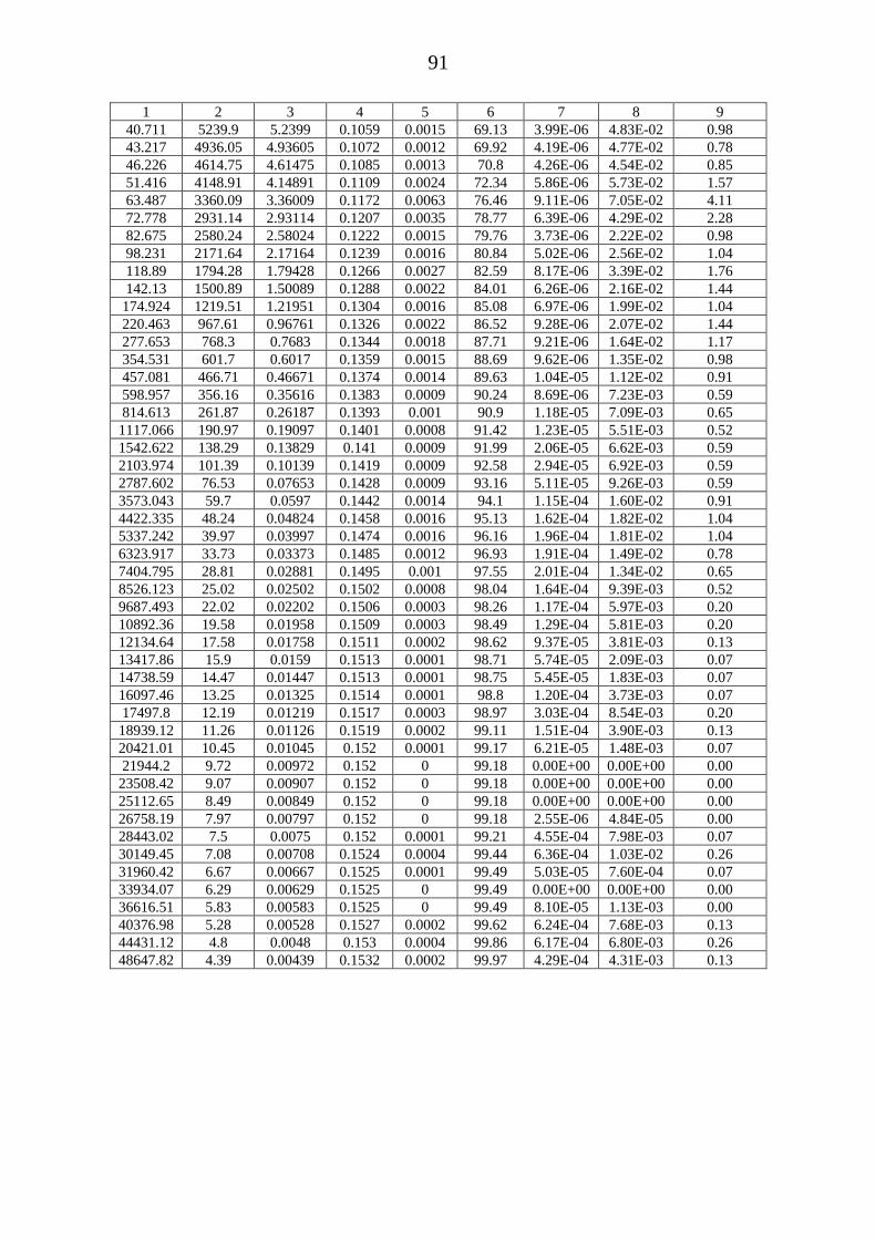
91
1 2 3 4 5 6 7 8 9
40.711 5239.9 5.2399 0.1059 0.0015 69.13 3.99E-06 4.83E-02 0.98
43.217 4936.05 4.93605 0.1072 0.0012 69.92 4.19E-06 4.77E-02 0.78
46.226 4614.75 4.61475 0.1085 0.0013 70.8 4.26E-06 4.54E-02 0.85
51.416 4148.91 4.14891 0.1109 0.0024 72.34 5.86E-06 5.73E-02 1.57
63.487 3360.09 3.36009 0.1172 0.0063 76.46 9.11E-06 7.05E-02 4.11
72.778 2931.14 2.93114 0.1207 0.0035 78.77 6.39E-06 4.29E-02 2.28
82.675 2580.24 2.58024 0.1222 0.0015 79.76 3.73E-06 2.22E-02 0.98
98.231 2171.64 2.17164 0.1239 0.0016 80.84 5.02E-06 2.56E-02 1.04
118.89 1794.28 1.79428 0.1266 0.0027 82.59 8.17E-06 3.39E-02 1.76
142.13 1500.89 1.50089 0.1288 0.0022 84.01 6.26E-06 2.16E-02 1.44
174.924 1219.51 1.21951 0.1304 0.0016 85.08 6.97E-06 1.99E-02 1.04
220.463 967.61 0.96761 0.1326 0.0022 86.52 9.28E-06 2.07E-02 1.44
277.653 768.3 0.7683 0.1344 0.0018 87.71 9.21E-06 1.64E-02 1.17
354.531 601.7 0.6017 0.1359 0.0015 88.69 9.62E-06 1.35E-02 0.98
457.081 466.71 0.46671 0.1374 0.0014 89.63 1.04E-05 1.12E-02 0.91
598.957 356.16 0.35616 0.1383 0.0009 90.24 8.69E-06 7.23E-03 0.59
814.613 261.87 0.26187 0.1393 0.001 90.9 1.18E-05 7.09E-03 0.65
1117.066 190.97 0.19097 0.1401 0.0008 91.42 1.23E-05 5.51E-03 0.52
1542.622 138.29 0.13829 0.141 0.0009 91.99 2.06E-05 6.62E-03 0.59
2103.974 101.39 0.10139 0.1419 0.0009 92.58 2.94E-05 6.92E-03 0.59
2787.602 76.53 0.07653 0.1428 0.0009 93.16 5.11E-05 9.26E-03 0.59
3573.043 59.7 0.0597 0.1442 0.0014 94.1 1.15E-04 1.60E-02 0.91
4422.335 48.24 0.04824 0.1458 0.0016 95.13 1.62E-04 1.82E-02 1.04
5337.242 39.97 0.03997 0.1474 0.0016 96.16 1.96E-04 1.81E-02 1.04
6323.917 33.73 0.03373 0.1485 0.0012 96.93 1.91E-04 1.49E-02 0.78
7404.795 28.81 0.02881 0.1495 0.001 97.55 2.01E-04 1.34E-02 0.65
8526.123 25.02 0.02502 0.1502 0.0008 98.04 1.64E-04 9.39E-03 0.52
9687.493 22.02 0.02202 0.1506 0.0003 98.26 1.17E-04 5.97E-03 0.20
10892.36 19.58 0.01958 0.1509 0.0003 98.49 1.29E-04 5.81E-03 0.20
12134.64 17.58 0.01758 0.1511 0.0002 98.62 9.37E-05 3.81E-03 0.13
13417.86 15.9 0.0159 0.1513 0.0001 98.71 5.74E-05 2.09E-03 0.07
14738.59 14.47 0.01447 0.1513 0.0001 98.75 5.45E-05 1.83E-03 0.07
16097.46 13.25 0.01325 0.1514 0.0001 98.8 1.20E-04 3.73E-03 0.07
17497.8 12.19 0.01219 0.1517 0.0003 98.97 3.03E-04 8.54E-03 0.20
18939.12 11.26 0.01126 0.1519 0.0002 99.11 1.51E-04 3.90E-03 0.13
20421.01 10.45 0.01045 0.152 0.0001 99.17 6.21E-05 1.48E-03 0.07
21944.2 9.72 0.00972 0.152 0 99.18 0.00E+00 0.00E+00 0.00
23508.42 9.07 0.00907 0.152 0 99.18 0.00E+00 0.00E+00 0.00
25112.65 8.49 0.00849 0.152 0 99.18 0.00E+00 0.00E+00 0.00
26758.19 7.97 0.00797 0.152 0 99.18 2.55E-06 4.84E-05 0.00
28443.02 7.5 0.0075 0.152 0.0001 99.21 4.55E-04 7.98E-03 0.07
30149.45 7.08 0.00708 0.1524 0.0004 99.44 6.36E-04 1.03E-02 0.26
31960.42 6.67 0.00667 0.1525 0.0001 99.49 5.03E-05 7.60E-04 0.07
33934.07 6.29 0.00629 0.1525 0 99.49 0.00E+00 0.00E+00 0.00
36616.51 5.83 0.00583 0.1525 0 99.49 8.10E-05 1.13E-03 0.00
40376.98 5.28 0.00528 0.1527 0.0002 99.62 6.24E-04 7.68E-03 0.13
44431.12 4.8 0.0048 0.153 0.0004 99.86 6.17E-04 6.80E-03 0.26
48647.82 4.39 0.00439 0.1532 0.0002 99.97 4.29E-04 4.31E-03 0.13

92
Figure B. 4Pore size distribution sample Akshabulak 45
Table B. 5Results of Mercury porosimeter of sample Akshabulak 206
Pressure
[PSI]
Pore
Diameter
[nm]
Pore
Diameter
[μm]
Volume
Intruded
[cc/g]
Delta
Volume
[cc/g]
Volume
Intruded
%
Dv(d)
[cc/(nm-
g)]
dV/d(log
[cc/g]
Pore size
Distribution,
%
1 2 3 4 5 6 7 8 9
0.818 260690.13 260.69013 0 0 0.00 4.81E-09 3.29E-03 0%
1.64 130068.63 130.06863 0.0018 0.0018 1.91 2.15E-08 6.48E-03 1.92%
2.464 86566.11 86.56611 0.003 0.0012 3.17 2.79E-08 5.53E-03 1.28%
3.166 67382.48 67.38248 0.0036 0.0007 3.88 5.21E-08 8.29E-03 0.75%
3.924 54366.09 54.36609 0.0045 0.0009 4.83 8.45E-08 1.07E-02 0.96%
4.746 44948.13 44.94813 0.0057 0.0011 6.05 1.70E-07 1.79E-02 1.17%
5.589 38171.43 38.17143 0.0075 0.0018 8.00 4.19E-07 3.76E-02 1.92%
6.438 33136.93 33.13693 0.0108 0.0033 11.49 7.58E-07 5.81E-02 3.52%
7.406 28803.53 28.80353 0.0144 0.0037 15.40 1.07E-06 7.23E-02 3.95%
8.584 24850.58 24.85058 0.0198 0.0053 21.06 1.34E-06 7.67E-02 5.66%
9.883 21584.41 21.58441 0.0239 0.0042 25.53 1.31E-06 6.53E-02 4.48%
11.23 18996.29 18.99629 0.027 0.0031 28.84 1.04E-06 4.55E-02 3.31%
12.667 16840.69 16.84069 0.029 0.002 30.96 9.62E-07 3.74E-02 2.13%
14.118 15109.63 15.10963 0.0306 0.0016 32.63 9.75E-07 3.41E-02 1.71%
15.513 13750.88 13.75088 0.0322 0.0016 34.31 1.09E-06 3.46E-02 1.71%
16.9 12622.72 12.62272 0.0333 0.0012 35.55 1.02E-06 2.99E-02 1.28%
18.652 11436.7 11.4367 0.0346 0.0013 36.94 1.31E-06 3.47E-02 1.39%
20.446 10433.38 10.43338 0.0363 0.0017 38.75 2.13E-06 5.15E-02 1.81%
22.168 9622.85 9.62285 0.0382 0.0019 40.76 1.81E-06 3.99E-02 2.03%
23.892 8928.78 8.92878 0.0392 0.001 41.79 1.56E-06 3.23E-02 1.07%
25.681 8306.62 8.30662 0.0402 0.001 42.9 1.61E-06 3.08E-02 1.07%
27.502 7756.65 7.75665 0.041 0.0008 43.73 1.20E-06 2.14E-02 0.85%
29.318 7276.05 7.27605 0.0416 0.0006 44.32 1.45E-06 2.44E-02 0.64%
31.258 6824.48 6.82448 0.0424 0.0008 45.22 1.90E-06 3.00E-02 0.85%
33.665 6336.62 6.33662 0.0433 0.0009 46.13 1.86E-06 2.72E-02 0.96%
36.429 5855.86 5.85586 0.0443 0.001 47.2 2.17E-06 2.94E-02 1.07%
39.078 5458.86 5.45886 0.0451 0.0009 48.11 2.02E-06 2.54E-02 0.96%
41.688 5117.15 5.11715 0.0458 0.0007 48.85 2.16E-06 2.55E-02 0.75%
44.464 4797.63 4.79763 0.0466 0.0007 49.64 2.54E-06 2.81E-02 0.75%
47.672 4474.82 4.47482 0.0473 0.0007 50.42 2.10E-06 2.17E-02 0.75%

93
1 2 3 4 5 6 7 8 9
52.747 4044.26 4.04426 0.0482 0.0009 51.39 2.08E-06 1.96E-02 0.96%
62.884 3392.33 3.39233 0.0498 0.0016 53.13 3.14E-06 2.49E-02 1.71%
74.597 2859.68 2.85968 0.0521 0.0022 55.53 4.88E-06 3.23E-02 2.35%
86.094 2477.79 2.47779 0.0539 0.0018 57.47 4.68E-06 2.69E-02 1.92%
100.707 2118.26 2.11826 0.0558 0.0019 59.49 5.72E-06 2.81E-02 2.03%
119.396 1786.68 1.78668 0.0579 0.0021 61.69 7.02E-06 2.92E-02 2.24%
143.955 1481.87 1.48187 0.0603 0.0025 64.32 8.72E-06 3.00E-02 2.67%
176.567 1208.17 1.20817 0.063 0.0027 67.15 1.09E-05 3.07E-02 2.88%
220.361 968.06 0.96806 0.0659 0.003 70.31 1.36E-05 3.07E-02 3.20%
277.58 768.51 0.76851 0.069 0.003 73.56 1.73E-05 3.09E-02 3.20%
348.852 611.5 0.6115 0.0723 0.0033 77.05 2.45E-05 3.49E-02 3.52%
433.309 492.31 0.49231 0.0756 0.0034 80.63 3.14E-05 3.59E-02 3.63%
529.679 402.74 0.40274 0.0787 0.0031 83.95 3.62E-05 3.37E-02 3.31%
637.817 334.46 0.33446 0.0812 0.0025 86.61 3.54E-05 2.73E-02 2.67%
761.325 280.2 0.2802 0.083 0.0018 88.51 3.42E-05 2.22E-02 1.92%
898.342 237.46 0.23746 0.0845 0.0015 90.15 3.64E-05 2.00E-02 1.60%
1052.767 202.63 0.20263 0.086 0.0015 91.71 5.19E-05 2.45E-02 1.60%
1215.234 175.54 0.17554 0.0876 0.0016 93.4 5.04E-05 2.03E-02 1.71%
1395.551 152.86 0.15286 0.0883 0.0007 94.19 2.95E-05 1.05E-02 0.75%
1636.917 130.32 0.13032 0.0892 0.0008 95.06 4.31E-05 1.30E-02 0.85%
1950.859 109.35 0.10935 0.0901 0.001 96.11 4.29E-05 1.08E-02 1.07%
2334.746 91.37 0.09137 0.0907 0.0006 96.74 2.44E-05 5.08E-03 0.64%
2816.027 75.75 0.07575 0.0909 0.0002 96.94 8.19E-06 1.43E-03 0.21%
3414.881 62.47 0.06247 0.0911 0.0002 97.12 1.74E-05 2.53E-03 0.21%
4119.473 51.78 0.05178 0.0913 0.0002 97.31 1.58E-05 1.90E-03 0.21%
4955.43 43.05 0.04305 0.0914 0.0001 97.45 9.40E-06 8.97E-04 0.11%
5926.138 36 0.036 0.0914 0 97.46 4.94E-06 4.41E-04 0.00%
7005.984 30.45 0.03045 0.0915 0.0001 97.6 4.34E-05 3.08E-03 0.11%
8126.076 26.25 0.02625 0.0917 0.0002 97.82 5.73E-05 3.52E-03 0.21%
9269.087 23.01 0.02301 0.092 0.0003 98.09 6.17E-05 3.23E-03 0.32%
10459.076 20.4 0.0204 0.0921 0.0001 98.16 2.36E-05 1.13E-03 0.11%
11687.966 18.25 0.01825 0.0922 0.0001 98.29 9.71E-05 4.12E-03 0.11%
12955.422 16.47 0.01647 0.0924 0.0002 98.49 5.57E-05 2.08E-03 0.21%
14262.372 14.96 0.01496 0.0924 0 98.52 3.93E-05 1.39E-03 0.00%
15606.601 13.67 0.01367 0.0926 0.0002 98.68 1.82E-04 5.78E-03 0.21%
16990.564 12.56 0.01256 0.0927 0.0002 98.89 1.48E-04 4.27E-03 0.21%
18416.477 11.58 0.01158 0.0929 0.0001 99.01 1.32E-04 3.54E-03 0.11%
19881.631 10.73 0.01073 0.093 0.0002 99.18 1.45E-04 3.55E-03 0.21%
21388.773 9.97 0.00997 0.0931 0.0001 99.24 6.98E-05 1.61E-03 0.11%
22936.35 9.30 0.0093 0.0931 0 99.28 4.60E-05 9.82E-04 0.00%
24523.342 8.70 0.0087 0.0931 0 99.31 1.91E-05 3.77E-04 0.00%
26152.555 8.16 0.00816 0.0932 0 99.32 1.06E-04 2.02E-03 0.00%
27861.605 7.66 0.00766 0.0933 0.0001 99.46 2.67E-04 4.71E-03 0.11%
29666.225 7.19 0.00719 0.0933 0.0001 99.52 2.71E-05 4.40E-04 0.11%
31418.43 6.79 0.00679 0.0933 0 99.52 0.00E+00 0.00E+00 0.00%
33195.992 6.43 0.00643 0.0933 0 99.52 1.48E-04 2.23E-03 0.00%
35171.09 6.07 0.00607 0.0935 0.0001 99.66 3.05E-04 4.24E-03 0.11%
38294.555 5.57 0.00557 0.0935 0 99.7 1.66E-05 2.15E-04 0.00%
42230.719 5.05 0.00505 0.0936 0.0001 99.75 2.53E-04 3.00E-03 0.11%
46355.223 4.60 0.0046 0.0937 0.0002 99.94 3.46E-04 3.65E-03 0.21%

94
Figure B. 5Pore size distribution sample Akshabulak 206
Table B. 6 Results of Mercury porosimeter of sample Akshabulak 500
Pressure
[PSI]
Pore
Diameter
[nm]
Pore
Diameter
[μm]
Volume
Intruded
[cc/g]
Delta
Volume
[cc/g]
Volume
Intruded
%
Dv(d)
[cc/(nm-
g)]
dV/d(log
[cc/g]
Pore size
Distribution,
%
1 2 3 4 5 6 7 8 9
0.818 340280.2 340.2802 0.0000 0.0000 0.00 4.81E-09 3.29E-03 0.00
1.64 239065.5 239.0655 0.0016 0.0016 1.91 2.15E-08 6.48E-03 1.52
2.464 182181.3 182.1813 0.0029 0.0013 3.17 2.79E-08 5.53E-03 1.28
3.166 153078.5 153.0785 0.0037 0.0008 3.88 5.21E-08 8.29E-03 0.75
3.924 117888.6 117.8886 0.0047 0.0010 4.83 8.45E-08 1.07E-02 0.96
4.746 99574.4 99.5744 0.0062 0.0016 6.05 1.70E-07 1.79E-02 1.50
5.589 73079.42 73.07942 0.0082 0.0020 8.00 4.19E-07 3.76E-02 1.92
6.438 62806.63 62.80663 0.0109 0.0026 11.49 7.58E-07 5.81E-02 2.52
7.406 52863.82 52.86382 0.0145 0.0037 15.40 1.07E-06 7.23E-02 3.55
8.584 44432.6 44.4326 0.0183 0.0038 21.06 1.34E-06 7.67E-02 3.66
9.883 38471.52 38.47152 0.0217 0.0034 25.53 1.31E-06 6.53E-02 3.28
11.23 33865.92 33.86592 0.0252 0.0034 28.84 1.04E-06 4.55E-02 3.31
12.667 29550.01 29.55001 0.0274 0.0022 30.96 9.62E-07 3.74E-02 2.14
14.118 26648.9 26.6489 0.0292 0.0018 32.63 9.75E-07 3.41E-02 1.71
15.513 23489.4 23.4894 0.0310 0.0018 34.31 1.09E-06 3.46E-02 1.71
16.9 21149.8 21.1498 0.0323 0.0013 35.55 1.02E-06 2.99E-02 1.28
18.652 18818.53 18.81853 0.0337 0.0014 36.94 1.31E-06 3.47E-02 1.39
20.446 16890.39 16.89039 0.0356 0.0019 38.75 2.13E-06 5.15E-02 1.82
22.168 15435.46 15.43546 0.0377 0.0021 40.76 1.81E-06 3.99E-02 2.03
23.892 14177.14 14.17714 0.0388 0.0011 41.79 1.56E-06 3.23E-02 1.07
25.681 13004.6 13.0046 0.0400 0.0011 42.9 1.61E-06 3.08E-02 1.07
27.502 11976.5 11.9765 0.0408 0.0009 43.73 1.20E-06 2.14E-02 0.85
29.318 11062.32 11.06232 0.0415 0.0007 44.32 1.45E-06 2.44E-02 0.64
31.258 10284.35 10.28435 0.0424 0.0009 45.22 1.90E-06 3.00E-02 0.85
33.665 9674.314 9.674314 0.0434 0.0010 46.13 1.86E-06 2.72E-02 0.96
36.429 9046.258 9.046258 0.0445 0.0011 47.2 2.17E-06 2.94E-02 1.07
39.078 8506.745 8.506745 0.0455 0.0010 48.11 2.02E-06 2.54E-02 0.96
41.688 7928.765 7.928765 0.0463 0.0008 48.85 2.16E-06 2.55E-02 0.75

95
1 2 3 4 5 6 7 8 9
44.464 7326.202 7.326202 0.0470 0.0008 49.64 2.54E-06 2.81E-02 0.75
47.672 6810.05 6.81005 0.0478 0.0008 50.42 2.10E-06 2.17E-02 0.75
52.747 6403.865 6.403865 0.0488 0.0010 51.39 2.08E-06 1.96E-02 0.96
62.884 6018.87 6.01887 0.0506 0.0018 53.13 3.14E-06 2.49E-02 1.71
74.597 5366.608 5.366608 0.0530 0.0024 55.53 4.88E-06 3.23E-02 2.35
86.094 4485.494 4.485494 0.0550 0.0020 57.47 4.68E-06 2.69E-02 1.92
100.707 3984.5 3.9845 0.0571 0.0021 59.49 5.72E-06 2.81E-02 2.03
119.396 3516.552 3.516552 0.0595 0.0023 61.69 7.02E-06 2.92E-02 2.24
143.955 3047.304 3.047304 0.0622 0.0028 64.32 8.72E-06 3.00E-02 2.67
176.567 2617.277 2.617277 0.0652 0.0030 67.15 1.09E-05 3.07E-02 2.88
220.361 2204.904 2.204904 0.0686 0.0033 70.31 1.36E-05 3.07E-02 3.20
277.58 1820.481 1.820481 0.0719 0.0033 73.56 1.73E-05 3.09E-02 3.20
348.852 1473.563 1.473563 0.0755 0.0037 77.05 2.45E-05 3.49E-02 3.52
433.309 1175.98 1.17598 0.0793 0.0038 80.63 3.14E-05 3.59E-02 3.63
529.679 932.412 0.932412 0.0827 0.0034 83.95 3.62E-05 3.37E-02 3.31
637.817 744.328 0.744328 0.0843 0.0015 86.61 3.54E-05 2.73E-02 1.47
761.325 602.017 0.602017 0.0856 0.0014 88.51 3.42E-05 2.22E-02 1.32
898.342 493.87 0.49387 0.0873 0.0017 90.15 3.64E-05 2.00E-02 1.60
1052.767 410.748 0.410748 0.0890 0.0017 91.71 5.19E-05 2.45E-02 1.60
1215.234 346.047 0.346047 0.0907 0.0018 93.4 5.04E-05 2.03E-02 1.71
1395.551 295.802 0.295802 0.0920 0.0012 94.19 2.95E-05 1.05E-02 1.17
1636.917 247.598 0.247598 0.0931 0.0011 95.06 4.31E-05 1.30E-02 1.07
1950.859 202.28 0.20228 0.0937 0.0007 96.11 4.29E-05 1.08E-02 0.64
2334.746 167.245 0.167245 0.0946 0.0009 96.74 2.44E-05 5.08E-03 0.85
2816.027 137.228 0.137228 0.0954 0.0008 96.94 8.19E-06 1.43E-03 0.75
3414.881 110.734 0.110734 0.0959 0.0006 97.12 1.74E-05 2.53E-03 0.53
4119.473 89.271 0.089271 0.0969 0.0010 97.31 1.58E-05 1.90E-03 0.96
4955.43 72.306 0.072306 0.0979 0.0010 97.45 9.40E-06 8.97E-04 0.96
5926.138 58.799 0.058799 0.0988 0.0009 97.46 4.94E-06 4.41E-04 0.85
7005.984 48.386 0.048386 0.0994 0.0006 97.6 4.34E-05 3.08E-03 0.53
8126.076 40.742 0.040742 0.1002 0.0008 97.82 5.73E-05 3.52E-03 0.75
9269.087 35.022 0.035022 0.1002 0.0000 98.09 6.17E-05 3.23E-03 0.03
10459.08 32.526 0.032526 0.1007 0.0005 98.16 2.36E-05 1.13E-03 0.48
11687.97 28.626 0.028626 0.1009 0.0002 98.29 9.71E-05 4.12E-03 0.24
12955.42 25.454 0.025454 0.1017 0.0007 98.49 5.57E-05 2.08E-03 0.71
14262.37 22.854 0.022854 0.1019 0.0002 98.52 3.93E-05 1.39E-03 0.24
15606.6 20.67 0.02067 0.1021 0.0001 98.68 1.82E-04 5.78E-03 0.14
16990.56 18.811 0.018811 0.1022 0.0001 98.89 1.48E-04 4.27E-03 0.14
18416.48 17.225 0.017225 0.1029 0.0007 99.01 1.32E-04 3.54E-03 0.67
19881.63 15.847 0.015847 0.1039 0.0010 99.18 1.45E-04 3.55E-03 0.99
21388.77 14.638 0.014638 0.1039 0.0000 99.24 6.98E-05 1.61E-03 0.03

96
Figure B. 6Pore size distribution sample Akshabulak 500

97
Appendix C
Appendix C presents the raw and calculated data of 3 polymer powder.
Table C 1 Mass fraction of the main substance
FP 3630 FP 5115 FP 5205
Mass of polymer before
drying, g 2.558 2.183 2.24
Mass of polymer after
drying, g 2.309 1.966 2.024
Mass fraction of the main
substance,% 90.27% 90.06% 90.36%
Table C 2 Hydrolysis degree
FP 3630 FP 5115 FP 5205
Mass of polymer, g 0.33 0.33 0.33
Volume of NaOH solution for
working sample titration, ml 8.15 4.5 5.6
Volume of NaOH solution for
working blank titration, ml 1.2 1.2 1.2
molar concentration of NaOH, mol/l 0.05 0.05 0.05
Polymer mass, g 0.106 0.107 0.107
Hydrolysis degree, % 25% 11% 15%

98
Table C 3 Intrinsic viscosity of sample FP3630
Polymer
drainage
time ,
sec. (t)
Average
polymer
drainage
time , sec. (t
avr)
Relative
viscosity
ηrel=tavr/
t0*
Specific
viscosity,
ηsp = ηrel
-1
Mass
concentration
of polymer
solution, g/dL
Ci
Reduced
viscosity,
dL/g ηsp/
Ci
C1
228.07
228.1 1.950 0.950 0.045
21.105 228.05
228.03
C2
206.6
206.6 1.767 0.767 0.037
20.955 206.7
206.6
C3
184.06
184.4 1.576 0.576 0.028
20.498 184.53
184.595
C4
163.62
163.6 1.398 0.398 0.020
20.258 163.56
163.5
C5
143.12
143.1 1.223 0.223 0.011 19.835 143.01
143.065
*t0=116.965
Figure C 1 Intrinsic viscosity of sample FP3630

99
Table C 4 Intrinsic viscosity of sample FP5115
Polymer
drainage
time ,
sec. (t)
Average
polymer
drainage
time , sec. (t
avr)
Relative
viscosity
ηrel=tavr/
t0*
Specific
viscosity,
ηsp =
ηrel -1
Mass
concentration
of polymer
solution, g/dL
Ci
Reduced
viscosity,
dL/g ηsp/
Ci
C1
225.15
225.2 1.930 0.930 0.045
20.66 225.25
225.2
C2
202.48
202.7 1.737 0.737 0.037
20.14 202.88
202.68
C3
181.59
181.8 1.558 0.558 0.028
19.8 181.98
181.75
C4
159.14
159.1 1.363 0.363 0.020
18.47 159.04
159.1
C5
139.99
139.9 1.199 0.199 0.011 17.65 139.86
139.75
*t0=116.965
Figure C 2 Intrinsic viscosity of sample FP5115

100
Table C 5Intrinsic viscosity of sample FP5205
Polymer
drainage
time ,
sec. (t)
Average
polymer
drainage
time , sec.
(t avr)
Relative
viscosity
ηrel=tavr/
t0*
Specific
viscosity,
ηsp =
ηrel -1
Mass
concentration
of polymer
solution, g/dL
Ci
Reduced
viscosity,
dL/g
ηsp/ Ci
C1
227.15
227.2 1.947 0.947 0.045
21.03 227.28
227.1
C2
204.28
204.4 1.752 0.752 0.037
20.54 204.41
204.58
C3
182.59
182.8 1.566 0.566 0.028
20.13 182.98
182.75
C4
159.94
160.0 1.371 0.371 0.020
18.85 159.99
159.94
C5
141.09
141.1 1.209 0.209 0.011 18.56 141.06
141.05
Figure C 3 Intrinsic viscosity of sample FP5205

101
Appendix D
Appendix D presents the Matlab code for calculation IPV and adsorbtion, and raw
data from experiment.
Matlab code
%read initial data A=dlmread('sample2_all.txt'); t=A(:,1); dp=A(:,2); res=A(:,3); %calculating viscosity, polymer concentration and norm.conc mu=(dp*6894.7573*3.14*((0.089/2)^4))/(8*414*(2/60))*1000; %viscosity C_pol=((mu-0.7735)/0.0041)/10^6; %polymer conc in g/cc C_pol_norm=C_pol/0.001513; %calculating conductivity, tracer concentration and norm.conc R=res*0.023854; %ohm/m cond =10./R;%mS/cm C_tr=(cond-72.062)/(0.7141*1000); %g/cc C_tr_norm=(C_tr-0.1)/(0.15-0.1); %calculating PV PV=t*(2/60)/9.71; %#ofPV %IPV t1=A(152:212,1); pv=t1*(2/60)/9.71; %#ofPV dp1=A(152:212,2); mu1=(dp1*6894.7573*3.14*((0.089/2)^4))/(8*414*(2/60))*1000; %viscosity c_pol=((mu1-0.7735)/0.0041)/10^6; %polymer conc in g/cc c_pol_norm=c_pol/0.001513; res1=A(152:212,3); R1=res1*0.023854; %ohm/m cond1 =10./R1; c_tr=(cond1-72.062)/(0.7141*1000); c_tr_norm=(c_tr-0.1)/(0.15-0.1); integral_polymer1 = trapz(pv,c_pol_norm); integral_tracer1 = trapz(pv,c_tr_norm); ipv=integral_tracer1-integral_polymer1; IPV=ipv/9.71; disp(['IPV = ',num2str(IPV) ]); % Absorption calculation

102
t2=A(1:59,1); % PV for absorption calculation pv1=t2*(2/60)/9.71; %#ofPV dp2=A(1:59,2); % polymer curve for absorption calculation mu2=(dp2*6894.7573*3.14*((0.089/2)^4))/(8*414*(2/60))*1000; %viscosity c_pol1=((mu2-0.7735)/0.0041)/10^6; %polymer conc in g/cc c_pol_norm1=c_pol1/0.001513; res2=A(1:59,3); %tracer curve for absorption calculation R2=res2*0.023854; %ohm/m cond2 =10./R2; c_tr1=(cond2-72.062)/(0.7141*1000); c_tr_norm1=(c_tr1-0.1)/(0.15-0.1); integral_polymer = trapz(pv1,c_pol_norm1); % area under polymer curve integral_tracer = trapz(pv1,c_tr_norm1); % area under tracer curve A=integral_tracer-integral_polymer; % difference in areas Ads=(A+ipv)*9.71*.001513/106.88; pol_abs=Ads*106.88; disp(['Adsorption1 = ',num2str(Ads), ' g/g' ]); disp(['Polymer absorbed1 = ',num2str(pol_abs), ' g' ]); figure(1); figure('Units','centimeters','color','w') subplot(2,2,1); plot(PV,C_pol_norm,PV,C_tr_norm) ylim([0 1]) legend('Cp = polymer production curve','Ct = tracer production curve') title('concentration vs PV','FontSize',16) xlabel('Pore Volume','FontSize',14) ylabel('Normalized Concentration','FontSize',14) legend('Location','SouthOutside') subplot(2,2,2); figure('Units','centimeters','color','w') plot(pv,c_pol_norm,pv,c_tr_norm) ylim([0 1]) title('IPV','FontSize',16) xlabel('Pore Volume','FontSize',14) ylabel('Normalized Concentration','FontSize',14) subplot(2,2,3); figure('Units','centimeters','color','w') plot(pv1,c_pol_norm1,pv1,c_tr_norm1); ylim([0 1]) title('Adsorption','FontSize',16) xlabel('Pore Volume','FontSize',14) ylabel('Normalized Concentration','FontSize',14)
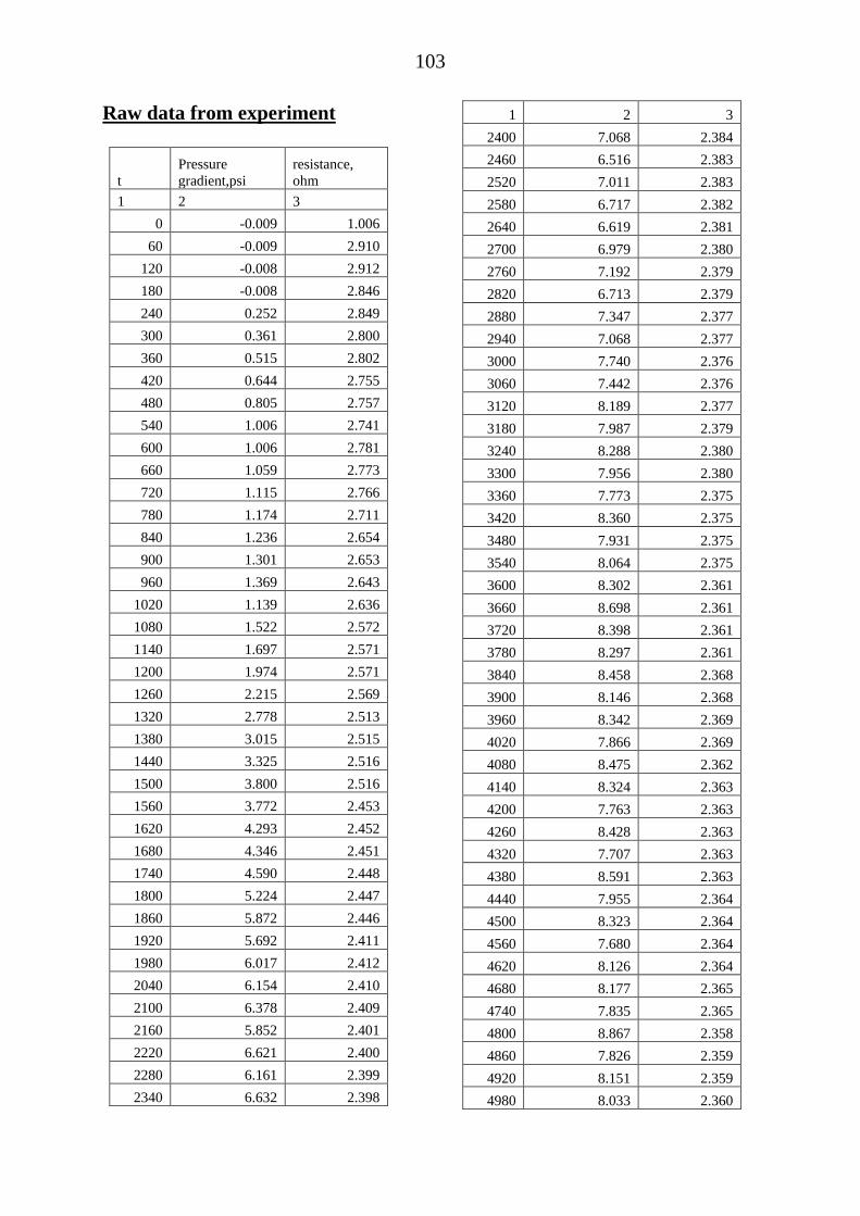
103
Raw data from experiment
t
Pressure
gradient,psi
resistance,
ohm
1 2 3
0 -0.009 1.006
60 -0.009 2.910
120 -0.008 2.912
180 -0.008 2.846
240 0.252 2.849
300 0.361 2.800
360 0.515 2.802
420 0.644 2.755
480 0.805 2.757
540 1.006 2.741
600 1.006 2.781
660 1.059 2.773
720 1.115 2.766
780 1.174 2.711
840 1.236 2.654
900 1.301 2.653
960 1.369 2.643
1020 1.139 2.636
1080 1.522 2.572
1140 1.697 2.571
1200 1.974 2.571
1260 2.215 2.569
1320 2.778 2.513
1380 3.015 2.515
1440 3.325 2.516
1500 3.800 2.516
1560 3.772 2.453
1620 4.293 2.452
1680 4.346 2.451
1740 4.590 2.448
1800 5.224 2.447
1860 5.872 2.446
1920 5.692 2.411
1980 6.017 2.412
2040 6.154 2.410
2100 6.378 2.409
2160 5.852 2.401
2220 6.621 2.400
2280 6.161 2.399
2340 6.632 2.398
1 2 3
2400 7.068 2.384
2460 6.516 2.383
2520 7.011 2.383
2580 6.717 2.382
2640 6.619 2.381
2700 6.979 2.380
2760 7.192 2.379
2820 6.713 2.379
2880 7.347 2.377
2940 7.068 2.377
3000 7.740 2.376
3060 7.442 2.376
3120 8.189 2.377
3180 7.987 2.379
3240 8.288 2.380
3300 7.956 2.380
3360 7.773 2.375
3420 8.360 2.375
3480 7.931 2.375
3540 8.064 2.375
3600 8.302 2.361
3660 8.698 2.361
3720 8.398 2.361
3780 8.297 2.361
3840 8.458 2.368
3900 8.146 2.368
3960 8.342 2.369
4020 7.866 2.369
4080 8.475 2.362
4140 8.324 2.363
4200 7.763 2.363
4260 8.428 2.363
4320 7.707 2.363
4380 8.591 2.363
4440 7.955 2.364
4500 8.323 2.364
4560 7.680 2.364
4620 8.126 2.364
4680 8.177 2.365
4740 7.835 2.365
4800 8.867 2.358
4860 7.826 2.359
4920 8.151 2.359
4980 8.033 2.360

104
1 2 3
5040 7.561 2.361
5100 8.182 2.362
5160 8.198 2.364
5220 7.928 2.365
5280 8.232 2.367
5340 7.956 2.368
5400 7.706 2.355
5460 8.317 2.357
5520 7.655 2.358
5580 8.141 2.360
5640 7.833 2.361
5700 8.372 2.363
5760 9.075 2.364
5820 8.023 2.353
5880 8.265 2.346
5940 8.629 2.345
6000 8.689 2.346
6060 8.853 2.343
6120 9.030 2.340
6180 8.643 2.343
6240 7.834 2.340
6300 8.307 2.340
6360 8.738 2.340
6420 8.263 2.340
6480 8.406 2.340
6540 8.212 2.340
6600 8.088 2.343
6660 8.479 2.341
6720 7.808 2.340
6780 8.964 2.340
6840 8.238 2.344
6900 8.308 2.342
6960 8.393 2.340
7020 8.881 2.345
7080 7.895 2.343
7140 8.121 2.343
7200 8.313 2.345
7260 8.421 2.351
7320 8.391 2.357
7380 8.681 2.353
7440 8.723 2.346
7500 8.212 2.354
7560 7.718 2.359
7620 8.111 2.347
1 2 3
7680 8.329 2.357
7740 7.546 2.352
7800 7.911 2.347
7860 8.106 2.350
7920 8.242 2.346
7980 7.803 2.351
8040 8.373 2.347
8100 8.282 2.340
8160 8.003 2.353
8220 8.307 2.346
8280 8.463 2.346
8340 8.485 2.353
8400 8.337 2.357
8460 8.261 2.353
8520 7.985 2.353
8580 8.140 2.353
8640 8.594 2.353
8700 8.715 2.360
8760 8.401 2.365
8820 8.666 2.367
8880 8.086 2.365
8940 8.692 2.369
9000 8.618 2.371
9060 8.586 2.374
9120 7.969 2.373
9180 8.370 2.378
9240 8.065 2.379
9300 8.258 2.382
9360 8.095 2.385
9420 8.304 2.387
9480 8.217 2.393
9540 7.609 2.394
9600 7.663 2.415
9660 8.027 2.416
9720 7.819 2.415
9780 7.241 2.414
9840 7.220 2.414
9900 7.164 2.412
9960 6.886 2.429
10020 7.170 2.472
10080 7.324 2.486
10140 6.603 2.478
10200 6.912 2.481
10260 6.922 2.500

105
1 2 3
10320 6.000 2.497
10380 5.734 2.493
10440 6.308 2.491
10500 5.361 2.489
10560 5.746 2.504
10620 5.103 2.523
10680 5.160 2.515
10740 5.142 2.515
10800 5.316 2.514
10860 4.870 2.536
10920 4.892 2.533
10980 3.450 2.536
11040 3.515 2.539
11100 2.742 2.541
11160 3.339 2.544
11220 2.479 2.604
11280 2.191 2.606
11340 1.481 2.608
11400 1.435 2.612
11460 1.177 2.619
11520 1.376 2.626
11580 1.419 2.627
11640 1.420 2.689
11700 0.846 2.692
11760 0.848 2.694
11820 0.816 2.714
11880 1.760 2.749
11940 2.102 2.751
12000 0.872 2.778
12060 1.196 2.804
12120 1.100 2.805
12180 1.865 2.806
12240 1.676 2.805
12300 1.133 2.809
12360 1.466 2.826
12420 0.224 2.858
12480 0.534 2.883
12540 0.086 2.892
12600 0.288 2.895
12660 0.357 2.900
Top Related