Download - air.unimi.it · Contents Introduction iii 1 Superintegrable Hamiltonian systems 1 1.1 The local geometry of a superintegrable system . . . . . . . . . . .3 1.2 The structure of the

Dipartimento di Matematica F.EnriquesCorso di dottorato di ricerca in Matematica

XXX Ciclo

On the stability of the perturbedcentral motion problem: a

quasiconvexity and a Nekhoroshevtype result

MAT/07

Tesi di dottorato di

Alessandra Fusè

Matricola

R11081-R32Relatore:

Prof. Dario Paolo Bambusi

Coordinatore del dottorato:

Prof. Vieri Mastropietro

ANNO ACCADEMICO 2016/2017

Contents

Introduction iii

1 Superintegrable Hamiltonian systems 1

1.1 The local geometry of a superintegrable system . . . . . . . . . . . 31.2 The structure of the base space and the bibration . . . . . . . . . 61.3 A Nekhoroshev type Theorem for superintegrable systems . . . . . 71.4 Proof of the Theorem . . . . . . . . . . . . . . . . . . . . . . . . . . 9

1.4.1 Normal form Theorem . . . . . . . . . . . . . . . . . . . . . 91.4.2 Semilocal stability estimates in the neighborhood of a res-

onant torus . . . . . . . . . . . . . . . . . . . . . . . . . . . 301.4.3 Dirichlet Theorem and semilocal stability . . . . . . . . . . 35

2 The spatial central motion problem 37

2.1 Statement of the structure theorem . . . . . . . . . . . . . . . . . . 372.2 Action angle coordinates for the planar case . . . . . . . . . . . . . 39

2.2.1 The construction of the action angle variables . . . . . . . . 412.3 From the planar to the spatial case . . . . . . . . . . . . . . . . . . 462.4 A Nekhoroshev type theorem . . . . . . . . . . . . . . . . . . . . . 482.5 The condition of quasiconvexity . . . . . . . . . . . . . . . . . . . . 492.6 Domains bounded below by a minimum . . . . . . . . . . . . . . . . 512.7 A new proof of Bertrand's Theorem . . . . . . . . . . . . . . . . . . 552.8 Domains bounded below by a maximum . . . . . . . . . . . . . . . 55

A The Bertrand's Theorem 62

A.1 Classical proof of Bertrand's Theorem . . . . . . . . . . . . . . . . . 62

B Dirichlet Theorem 67

C Technical lemmas and results 70

C.1 Ehresmann bration lemma . . . . . . . . . . . . . . . . . . . . . . 70C.2 Some useful lemmas . . . . . . . . . . . . . . . . . . . . . . . . . . 70

i

CONTENTS ii

D Normal forms and other results 76

D.1 Birkho normal form . . . . . . . . . . . . . . . . . . . . . . . . . . 76D.2 Burgers equation . . . . . . . . . . . . . . . . . . . . . . . . . . . . 83D.3 Domains bounded below by a maximum of the eective potential . 85

E MathematicaTM computation 91

Bibliography 108

Introduction

This thesis is devoted to the study of the dynamics of small perturbations of thespatial central motion.

In particular, we are interested in proving a Nekhoroshev type theorem for it.The point is that Nekhoroshev's theorem applies to perturbations of integrable

systems whose Hamiltonian when written in the action angle coordinates is steep.Now such a property, in its original form, is always violated in the spatial centralmotion since it is a superintegrable system and its Hamiltonian turns out to bealways independent of one of the actions.

For degenerate systems, stability results have been obtained by Nekhoroshevin the papers ([Nek77, Nek79]) and, subsequently, by Niedermann (see [Nie96]),Guzzo and Morbidelli, see [GM96, Guz99] in which the authors apply exponentialstability results in order to study the stability of the planetary problem.

A general Nekhoroshev theory for superintegrable systems has been developedalso by Fassò [Fas95], [Fas05] (see also Blaom in [Bla01]), and the main knownresult is that a weaker version of Nekhoroshev's theorem ensuring almost conser-vation of the two actions on which the Hamiltonian depends holds provided theHamiltonian is a convex function of these two actions. We remark that it is quiteclear how to extend Fassò's theory to the case of steep dependence on the twoactions.

The rst goal of the thesis is to write a complete proof of Nekhoroshev's the-orem for superintegrable systems under the assumption that the Hamiltonian isquasiconvex in the actions on which it actually depends. This is done by gener-alizing the proof by Lochak (see [Loc92]) which is much simpler then the originalone by Nekhoroshev (see [Nek77, Nek79]) (the one extended by Fassò ).

Then, we tackle the problem of proving that the Hamiltonian in action anglevariables is quasiconvex. This is far from trivial since the expression of the Hamilto-nian depends on the form of the potential and one expects that quasiconvexityholds under some conditions on the potential. The main technical result of thethesis is that actually there are only two central potentials corresponding to whichthe Hamiltonian is not quasiconvex, namely, the Harmonic and the Keplerian one.

We are now going to state in a precise way the main result of the thesis.

iii

INTRODUCTION iv

In Cartesian coordinates, the Hamiltonian of the spatial central motion is givenby

H(x,p) =|p|2

2+ V (|x|) , (1)

p ≡ (px, py, pz) , x ≡ (x, y, z) , |x| :=√x2 + y2 + z2 ,

where V is the potential that we assume to be analytic. Furthermore, we assumethat it fullls the following assumptions

(H0) V : (0,+∞)→ R is a real analytic function.

(H1) −`∗ :=1

2limr→0+

r2V (r) > −∞

(H2) ∃r > 0 : r3V ′(r) > max 0, `∗,

(H3) ∀` > max 0, `∗ the equation (in r) r3V ′(r) = ` has at most a nite numberof solutions.

Remark 0.0.1. (H1) ensures that there are no collision orbits provided the angularmomentum is large enough; (H2) ensures that the eective potential has at leastone strict minimum so that the domain of the actions is not empty; nally (H3)ensures that the domain of the actions is not too complicated.

Remark 0.0.2. For example any analytic potential of Schwartz class such thatbounded orbits exist fullls the assumptions.

Dene the total angular momentum (L1, L2, L3) ≡ L := x × p and denote byL :=

√L2

1 + L22 + L2

3 its modulus.

Let P(3)A ⊂ R6 be a compact subset of the phase space invariant under the

dynamics of H,

Theorem 0.0.1. Assume that V is neither Harmonic nor Keplerian; then thereexists a set K(3) ⊂ P(3)

A , which is the union of nitely many analytic hypersurfaces,

with the following property: let P : P(3)A → R be a real analytic function. Let

C(3) ⊂ P(3)A \K(3) be compact and invariant for the dynamics of H; then there exist

positive ε∗, C1, C2, C3, C4 with the following property: for |ε| < ε∗, consider thedynamics of the Hamiltonian system

Hε := H + εP

then, for any initial datum in C(3) one has

|L(t)− L(0)| ≤ C1ε1/4 , |H(t)−H(0)| ≤ C2ε

1/4 , (2)

for|t| ≤ C3 exp(C4ε

−1/4) . (3)

INTRODUCTION v

An immediate consequence of the above theorem is that the particle's orbitsare conned between two spherical shells centered at the origin.

We now discuss the proof of the result. As anticipated above, the Hamiltoniansystem associated to the spatial central motion problem belongs to the class ofsuperintegrable systems, namely, systems which admit a number of independentintegrals of motion larger than the number of degrees of freedom. The mainproperty of such systems is that, under some technical conditions, they admitgeneralized action angle coordinates and the Hamiltonian turns out to depend ona number of actions strictly smaller than the number of degrees of freedom.

Furthermore, in general, the level set of the actions is a nontrivial manifoldwhich cannot be covered by only one system of coordinates. As pointed out byFassò, this poses nontrivial problems for the development of the proof of Nek-horoshev's theorem. The geometrical idea introduced by Fassò in order to proveNekhoroshev's theorem is that, even if normal form theory is classically developedusing coordinates, in the framework of superintegrable systems, the expressionsobtained in the chart, as well as the normalizing transformation, glue togetherand give a function and a normal form which are dened "semilocally". By thiswe mean on the manifold obtained by considering the union for I in a small openset of the level sets of I, where I are the actions of the system.

In Chapter 1 of this thesis, we show how to use these ideas in order to adaptLochak's proof of Nekhoroshev's theorem to superintegrable systems. We alsodetail the proof for the case of quasiconvex systems, which, as far as we know, wasnot treated explicitly in literature. We remark that in order to get the proof onlysome of the ideas by Fassò are needed.

Then (Chapter 2), we come to a detailed study of the central motion problem.First, we apply the general geometric theory of superintegrable systems to thespatial central motion. To do so, we rst analyze the planar central motion andshow that we can reduce our analysis to this case. Thus, it turns out that thegeneral Nekhoroshev's theorem proved in Chapter 1 applies if the Hamiltonian ofthe planar central motion is quasiconvex. Thus we study it.

In polar coordinates, the Hamiltonian of the planar central motion problemhas the well known form

H(r, pr, pθ) =p2r

2+

p2θ

2r2+ V (r) . (4)

The main remark is that, in the case of systems with 2 degrees of freedom, thequasiconvexity condition turns out to be equivalent to the nonvanishing of the so

INTRODUCTION vi

called Arnol'd determinant, namely,

D = det

∂2h

∂I2

(∂h

∂I

)T∂h

∂I0

,

where h is the unperturbed Hamiltonian written in the action variables. Moreover,in the analytic case, the Arnol'd determinant is an analytic function, thus only twopossibilities occur: either it is a trivial analytic function, or it is always dierentfrom zero except on an analytic hypersurface.

Recall now that the two actions of the planar system are the angular momentumvector I2 := pθ and the action I1 of the reduced system, that is, the system withHamiltonian (4) where pθ plays the role of a parameter. The action I1 depends onthe form of the eective potential, namely,

Veff (r, p2θ) :=

p2θ

2r2+ V (r) .

We use the assumptions (H0)− (H3) in order to study quite precisely the domainof I1, I2.

More precisely, we start by proving that, correspondingly to almost every valueof I2, the eective potential has only nondegenerate critical points. Then, we x avalue of the angular momentum I2 and we proceed with the standard constructionof the action I1.

A simple analysis shows that the domain of denition of the action I1 is theunion of some open connected regions Ej of the phase-space. The regions Ej canbe classied into two categories according to the nature of the critical points ofVeff contained in their closure. Precisely, we will distinguish between the regions

E (1)j whose closure contains a minimum of the eective potential and the regions

E (2)j whose closure, instead, does not contain a minimum but contains necessarilya maximum of the eective potential.

Then, the heart of the proof is based on the study of the asymptotic behaviorof the Arnol'd determinant at circular orbits corresponding to the critical pointsof Veff and goes dierently in the two kinds of regions.

Specically, we rst consider the regions E (1)j and we compute the rst terms of

the expansion of the Hamiltonian at the minima by computing the rst terms ofthe Birkho normal form of the eective system in terms of the derivatives of thepotential. This has been done extending the procedure used by Féjoz in [FK04]who actually did the computation at order 4. Here we go at order 6. Then, we usesuch an expansion in order to compute the rst terms of the Arnol'd determinant

INTRODUCTION vii

and to show that it is a nontrivial function, except in the Harmonic and Kepleriancases.

Precisely, we get that the rst two terms of the expansion of the Arnol'd de-terminant vanish identically if the potential V (r) fullls a couple of dierentialequations. Then, we search for the common solutions of these two equationsand we obtain that they are the Keplerian and the Harmonic potentials. Thisis a quite heavy computation and is done by the help of a symbolic manipulator(MathematicaTM). The corresponding computation is reported in Appendix E.

Then, we consider the second regions E (2)j . We prove that if such a region exists

then, the Arnol'd determinant diverges at its boundary and thus it is a nontrivialfunction of the actions.

The result is obtained by exploiting the fact that the action I1 at the maximumadmits an asymptotic expansion of the form

I1 = −Λ(E − V0, I2) ln(E − V0) +G1(E − V0, I2) , (5)

where we denote by V0 the value of the eective potential at the maximum, by Ethe energy level while G1 and Λ are two analytic functions. Moreover, Λ has azero of order 1 in (0, I2). Secondly, from this expansion, we derive the asymptoticbehavior of the Arnol'd determinant at the maximum and prove that it divergesat such a point. In the thesis we prove formula (5) exploiting a normal formresult by Giorgilli [Gio01]. This formula also appears in [BC17]. In this work theauthors apply a KAM type theorem to a nearly-integrable Hamiltonian systemunder suitable conditions. Previously, such a formula also appeared in the workby Neishtadt [Nei87].

To conclude we remark that our result, showing some peculiarities of the Har-monic and the Keplerian potentials, of course reminds Bertrand's theorem. Ac-tually our analysis of the minima of the eective potential is a renement of thatused in the proof of Bertrand's theorem and can be used to get a new proof ofsuch a theorem (see Section 2.7). In Appendix A, we also added a proof of such aresult.

The results discussed here have been the object for two papers: [BF17] and[BFS17].

Chapter 1

Superintegrable Hamiltonian

systems

The aim of this section is the development of a Hamiltonian perturbation theoryfor superintegrable sytems, that we are now going to dene

Denition 1.0.1. Let (H,M,ω) a Hamiltonian system, where H : M 7→ R isthe Hamiltonian function, M a 2d-dimensional symplectic manifold and ω thesymplectic form.

Let us consider k functions F1, . . . , Fk : M 7→ R. Dene a map F := (F1, . . . , Fk) :M 7→ Rk and consider the function F : M 7→ F (M) :=M⊂ Rk.

We say that the functions Fj constitute a maximal set of independent integralsof motion if the following conditions are satised

1. H,Fj = 0 , ∀j = 1, . . . , k ,

2. dF1, . . . , dFk are linearly independent at every point of M ,

3. for any other function G such that H,G, the dierentials dG, dF1, . . . , dFkare linearly dependent .

Remark 1.0.3. In a superintegrable system, the Fj's are the elements of a maximalset of independent integrals of motion, F is a surjective submersion since the rankof the Jacobian matrix associated is constant at every point of M∗ and equal to2d − n. Furthermore, the bers are the level sets F−1(c) := x ∈ M : Fl(x) =cl, l = 1, . . . , k , cl ∈ R .

Denition 1.0.2. Let F1, . . . , Fk be a maximal set of independent integrals ofmotion and suppose that there exists real analytic functions Pi,j : M 7→ R suchthat

Fi, Fj = Pi,j F, i, j = 1, . . . , k .

The k × k matrix whose entries are the functions Pi,j is the Poisson matrix.

1

CHAPTER 1. SUPERINTEGRABLE HAMILTONIAN SYSTEMS 2

Denition 1.0.3. Let us consider a Hamiltonian system and let F1, . . . , Fk be amaximal set of independent integrals of motion admitting a Poisson matrix. Thesystem is said to be superintegrable if k > d and the Poisson matrix has constantrank equal to 2k − 2d at every point ofM.

Denition 1.0.4. If k = d, the Hamiltonian system is completely integrable.

Superintegrable systems are characterized by the fact that the number of in-dependent integrals of motion is greater than the number of degrees of freedom.They are also known as degenerate systems due to the fact that the correspondingHamiltonian, when written in generalized action angle coordinates, does not de-pend on all the actions. A property that we will describe in detail below. Systemsof that kind are frequent in literature: the Euler-Poinsot problem for the rigidbody motion and the spatial central motion problem are two important examples.

Example 1. The central motion problem.Let us consider the spatial central motion problem, that is, a particle in R3

moving under a central potential. The Hamiltonian describing the system writtenin Cartesian coordinates is

H(x,p) =|p|2

2+ V (|x|) ,

p ≡ (px, py, pz) , x ≡ (x, y, z) , |x| :=√x2 + y2 + z2 .

Dene the total angular momentum (L1, L2, L3) ≡ L := x × p and denote byL :=

√L2

1 + L22 + L2

3 its modulus.This system admits four integrals of motion, namely, the energy E of the system

and the three components (L1, L2, L3) of the angular momentum vector. Providedwe restrict to a subset M∗ of the phase-space in which the modulus of the angularmomentum vector is non zero and the motion is bounded, they constitute a maximalset of independent integrals of motion.

Furthermore, if we compute the Poisson matrix associated, we obtain

P =

0 0 0 00 0 L3 −L2

0 −L3 0 L1

0 L2 −L1 0

,

which has rank 2 at every point of F (M∗).

The main feature of these systems is that the variables corresponding to thedegenerate directions do not contribute to the dynamics. Thus, the dimension ofthe tori lled by the ow is smaller than the number of degrees of freedom and it


implies that the structure of the phase space is ner than the one which arises inthe case of a complete integrable system.

In detail, in the rst part of the current section, we introduce the double bra-tion structure of the phase-space by presenting rst the locally trivial bration inn-dimensional tori given by the adaptation of the Liouville-Arnol'd constructionto the superintegrable case and, then, we will deal with a second bration arisingfrom a particular choice of a symplectic atlas adapted to the rst bration. Thestructure of the double bration has been studied in detail in the works [Nek72],[KM12], [MF78], [Fas95] and [Fas05].

Secondly, we will present a stability result, a general Nekhoroshev type the-orem for superintegrable Hamiltonian systems whose corresponding Hamiltonianis quasiconvex when written in the action angle variables.

1.1 The local geometry of a superintegrable system

We begin with a couple of denitions which are useful in the description of thephase space of a superintegrable system.

Denition 1.1.1. Let M be a smooth manifold of dimension 2d. A foliation ofdimension n on M is an atlas Uj, φjj∈J on M with the following properties

1. ∀p ∈ M there exists a local chart Uj, φj such that φ(Uj) = V ′ × V ′′, withV ′ ⊂ Rn and V ′′ ⊂ R2d−n open subsets.

2. if Uj, φj and Uk, φk are such that Uj∩Uk 6= 0 then the transition functionsφk φ−1

j : φj(Uj ∩ Uk) 7→ φk(Uj ∩ Uk) are of the form

φk φ−1j (x, y) = (f1(x, y), f2(y)) , (x, y) ∈ Rn × R2d−n .

The leaves of the foliation are locally described by sets of the form

yn+1 = cn+1, . . . , ym = cm ,

with ck ∈ R which are n-dimensional submanifolds of M .

Denition 1.1.2. Let S be a manifold. A bration (or ber bundle) with ber Son a manifold N is a C∞ surjective map f : M 7→ N between a manifold M (thetotal space of the bration) and the manifold N (the base space of the bration)such that the following conditions are satised

1. ∀p ∈ N f−1(p) := Mp∼= S


2. every ber of f admits local trivializations, that is, ∀p ∈ N there exist aneighborhood U of p ∈ N and a dieomorphism ψ : f−1(U) 7→ U × S suchthat the following diagram commutes

f−1(U)ψ //

f%%

U × S

π1

U

Let (H,M,ω) be a superintegrable Hamiltonian system whereM is a 2d-dimensionalsymplectic manifold. Let us consider a maximal set of independent integrals ofmotion

F1, . . . , F2d−n : M∗ ⊂M → R ,

with n < d, dened on an open subset M∗ ⊂ M . We remind the reader that weare considering a superintegrable system, thus, the number of constants of motionis greater than the number of degrees of freedom.Let us consider the map F := (F1, . . . , F2d−n) : M∗ 7→ F (M∗) ⊂ R2d−n. FromRemark 1.0.3 we deduce that the map F is a surjective submersion whose bersare the level sets F−1(c) = x ∈M∗ : Fk(x) = ck , k = 1, . . . , 2d− n, ck ∈ R.

Thus, if we suppose that the bers are compact and connected than it followsfrom Ehresmann bration lemma1 that the map F is a bration in the sense ofdenition 1.1.2.

The main result which describes the local geometry of a superintegrable Hamilto-nian system is a generalization of the Liouville-Arnol'd Theorem for complete in-tegrable systems. Dierent versions of this theorem can be found in the works[Nek72], [MF78], [Fas95] and [Fas05]. The version we refer to in this work is theone given by Fassò in [Fas05] (or [Fas95]). The result is the following

Theorem 1.1.1. Let (H,M,ω) be a 2d-dimensional superintegrable Hamiltoniansystem. Let F := (F1, . . . , F2d−n) : M∗ ⊂ M 7→ F (M∗) :=M⊂ R2d−n with n < dbe a map whose components belong to a maximal set of independent integrals ofmotion with the property that the rank of the Poisson matrix P is everywhereconstant and equal to 2d− 2n.Moreover, assume that the level sets, that is, the bers of the map F are compactand connected.Then,

1. Every ber of F is dieomorphic to a n-dimensional torus Tn

1For details, see Appendix C


2. Every ber of F has a neighborhood U ⊂M∗ endowed with a dieomorphism

b× α : U→ B × Tn, B = b(U) ⊂ R2d−n (1.1)

such that the level sets of F coincide with the level sets of b and, writing b =(I1, · · · , In, p1, · · · , pd−n, q1, · · · , qd−n), the symplectic form ω can be writtenas

ω|U =n∑j=1

dIj ∧ dαj +d−n∑k=1

dpk ∧ dqk .

This result states that the submanifold M∗ presents a structure of a brationwhose bers are dieomorphic to n-dimensional invariant tori Tn. Moreover, in aneighborhood of each torus, thus locally, there exists a set of generalized action-angle coordinates adapted to the bration.

Denition 1.1.3. The coordinates b× α = (I, p, q, α) are called a set of general-ized action-angle coordinates since the variables (p, q) are not a couple of actionangle coordinates.

Lemma 1.1.1. Let H|U be a local representative of the Hamiltonian H in a localsystem of generalized action angle coordinates

b× α = (I1, · · · , In, p1, · · · , pd−n, q1, · · · , qd−n, α1, . . . , αn) .

Then, H|U depends on the actions (I1, . . . , In) only.

Proof. Let us consider the 2d−n integrals of motion Fj: they constitute a systemof coordinates in U which is independent of the variables α.

Thus, since Fj depend only on (I, p, q) and, moreover, are in involution withthe Hamiltonian, being integrals of motion, it follows

H|U , Fj = 0 ⇒ H|U , I = H|U , p = H|U , q = 0 ,

and, in particular,∂H|U∂α

=∂H|U∂q

=∂H|U∂p

= 0 .

It implies thatH|U= H|U(I) .

The following lemma gives the connection between dierent sets of generalizedaction-angle coordinates.


Lemma 1.1.2. Let us consider a symplectic atlas formed by generalized actionangle coordinates and let U, b × α and U ′, b′ × α′ be two charts such thatU ∩ U ′ 6= 0.Then, the transition functions dened in each connected component of the inter-section of the two chart domains have the following form,

I ′ = ZI + z (1.2)

(p′, q′) = G(I, p, q) (1.3)

α′ = Z−Tα + F(I, p, q) (1.4)

with F ,G analytic functions, z ∈ Rn and Z ∈ SL±(Z, n).

For the proof see for instance [Fas05].

1.2 The structure of the base space and the bi-

bration

As we have already underlined before, the dierence between integrable and su-perintegrable system consists mainly of the fact that the tori on which we havequasi-periodic motion have dimension smaller than the dimension of the base spaceof the bration.

We now describe this structure more in detail.Let us consider the bration F : M∗ 7→ M and a symplectic atlas Uj, bj ×

αjj∈J of generalized action angle coordinates. We can notice that this atlasinduces an atlas for the base space manifoldM with chart domains Bj =: F (Uj)

and coordinates given by bj = (Ij, pj, qj) = π1 (bj × α) F−1 = bj F−1 wherewe have denoted as π1 the projection onto the rst coordinate, as showed in thediagram below

Uj

F

bj×αj //

bj

((

Bj × Tn

π1

Mj

bj

// Bj

Thus, the family Bj, bjj represents an atlas for the base spaceM. Let us nowstudy this manifold in detail.

From Lemma 1.1.2, we notice that the transition functions for the actions involveonly themselves meaning that we have a subset of the coordinate system whichtransforms independently from the other coordinates.


Due to the structure ofM one can dene a manifold A as follows: the rangeof its charts are given by the projection on the rst factor of Bj and the transitionfunctions are dened by (1.2). A is called the action space.

Then, of course, one can dene a map

F :M→A

which is a foliation (Def. 1.1.1) whose leaves are the set F−1(a) with a ∈ A.

Remark 1.2.1. Since the frequency of the quasi-periodic motion on the tori de-pends on the value of the actions, it follows that the tori based on the same leafsupport motions with the same frequency.

Hypothesis 1. We assume that the map F :M→A denes a bration.

Thus, we have that M∗ has the structure of a bibration

M∗ F−→M F−→ A ,

and, furthermore, every ber F−1(a) is isomorphic to a given manifold Q. Forexample, in the situation of the spatial central motion problem, we will see thatQ ∼= S2.

We conclude this section with the following lemma which tell us that the trans-ition functions can be given an easier form if we make a smart choice of the atlasof the bration.

Lemma 1.2.1. If the action space A is simply connected, then there exists anatlas with transition functions of the form

I ′ = I

(p′, q′) = G(I, p, q)

α′ = α + F(I, p, q)

For details see [Fas95].In particular, we remark that, for any small enough open set V ⊂ A one has

F−1(V) ∼= V ×Q .

1.3 A Nekhoroshev type Theorem for superinteg-

rable systems

The aim of this section is to develop a Nekhoroshev type theorem for a perturbationof a superintegrable Hamiltonian system with quasiconvex Hamiltonian. Precisely,


we will show that the actions of such a system are approximately conserved fortimes which are exponentially long with the inverse of the perturbation parameter.

The main problem we have to tackle in order to get this result is related tothe fact that, as we have seen in the previous sections, each system of action-anglecoordinates is in general not globally dened. This is particularly evident when Qis compact.

This diculty was solved by Fassò who adapted Nekhoroshev's proof of Nek-horoshev Theorem to this situation. Here we adapt Lochak's proof to this context:in particular, it simplies considerably the result. A proof based on Lochak'smethod was already given in Blaom. In this work, the author produces an ab-stract version of the Nekhoroshev Theorem for perturbations of non-commutativeintegrable Hamiltonian systems. The result follows under the hypothesis that theunperturbed Hamiltonian satises certain properties of analyticity and convexity.

In particular, our proof is given for the case of quasiconvex systems in the sensethat we will explain in a while.

Before stating the main result, we recall a couple of denitions.

Denition 1.3.1. Let M∗ be a 2d-dimensional real manifold. An analytic struc-ture on M∗ is an atlas with the property that all the transition functions are realanalytic. The pair (M∗, Uj, φj)j∈J is called a real analytic manifold.

Let M∗ F−→ M F−→ A be the bibration described previously with M∗ a 2d-dimensional real analytic manifold endowed with an atlas whose transition func-tions satisfy the hypothesis of Lemma 1.2.1 and let H : M∗ 7→ R be the unper-turbed Hamiltonian of the corresponding superintegrable system.

Let us introduce a function h : A 7→ R dened on the action space such thatH = h F1, where F1 = F F .

Lemma 1.3.1. The function h : A 7→ R is a real analytic function on the wholeA.

Proof. The result follows from the fact that the map which introduces the set ofgeneralized action angle coordinates is an analytic dieomorphism.

Finally, we will make use of the following property of quasiconvexity.

Denition 1.3.2. A function h : A 7→ R is said to be quasiconvex at a point I∗ ifthe inequality

〈η, ∂2h

∂I2(I∗)η〉 ≥ c ‖η‖2

holds for any η such that 〈∂h∂I

(I∗), η〉 = 0.

Our main result is stated in the following theorem


Theorem 1.3.1. Let us consider a bibration M∗ F−→ M F−→ A endowed with anatlas of generalized action-angle coordinates Uj, φjj∈J of the form specied inLemma 1.2.1. Let h : A 7→ R and f : M∗ 7→ R be two real analytic functions,dene H := h F1, where F1 = F F , and assume that h is quasiconvex in A.Let C ⊂ M∗ be compact and invariant for the dynamics of H; then, there existpositive constants ε∗, C1, C2, C3 with the following property: for |ε| < ε∗ considerthe dynamics of the Hamiltonian system

Hε := H + εf

then, for any initial datum in C one has

‖I(t)− I(0)‖ ≤ C1ε1

2n ,

for all times t satisfying| t |≤ C2exp(C3ε

− 12n ) .

1.4 Proof of the Theorem

1.4.1 Normal form Theorem

The rst part of the proof concerns the construction of a semilocal normal form.We start by choosing an appropriate norm with which we measure the size ofthe functions and of their vector elds. Then, we will dene and complexify thedomain on which we will construct our normal form.

The methods used in the construction of the normal form are a slight modic-ation of the ones of [Loc92]. The main point is that the normal form we providehere is semilocal, meaning that it is well dened on a neighborhood of a ber ofthe action space, namely, using the notation of the previous sections, in

F−1(F−1(V)) ,

with V ⊂ A a small open subset.The result follows from the fact that the time averaging of a function and the

function which generates the transformation which puts the Hamiltonian in normalform are dened semilocally.

However, the quantitative estimates have to be constructed locally by consid-ering in each chart the local representative of the semilocal normal form.

Preliminaries and notations

Let us consider the bibration M∗ F−→ M F−→ A where (M∗, Uj, φjj) is the 2d-dimensional analytic manifold with the atlas chosen as in Lemma 1.2.1 with

φj : Uj 7→ Bj × Tn


given by φ(z) = (Ij, pj, qj, αj) , z ∈M∗.We choose to work semilocally in the sense that we work close to a single value

of the action. Thus, let us x a value I∗ ∈ A. To be more precise, for ρ > 0, wedene the ball

Bρ(I∗) = I ∈ Rn : ‖I − I∗‖ < ρ .Then, we dene

MI∗,ρ := F−1(F−1(Bρ(I∗))) ,and we will construct a normal form in such a submanifold. Remark that MI∗,ρ

∼=Bρ(I∗)× P where P is a suitable manifold.

At the end of the procedure, we will get a result valid over the whole of M∗ bychoosing a suitable collection of I∗j and ρj such that

M∗ = ∪jMI∗j ,ρj.

We x an atlas of generalized action angle coordinates (I, p, q, α) in MI∗,ρ. Denoteby Uj ⊂ R2d the range of the jth chart and remark that the I's coincide for all thecharts while (p, q, α) are coordinates on P . In order to measure distances on Uj,we will introduce two parameters R > 0 and σ > 0 and we introduce the norm

‖(I, p, q, α)‖ :=1

R

n∑i=1

|Ii|+ supj

R|αj|σ

+

√√√√d−n∑l=1

(|pl|2 + |ql|2) . (1.5)

Let f : MI∗,ρ 7→ R be a function. We will say that f ∈ Cω(ρ) if its local repres-entative fj in any chart is a real analytic function which extends to a boundedcomplex analytic function on

Uρj := ∪z∈UjBρ(z) ,

where z = (I, p, q, α).

Denition 1.4.1. Let fj be the local representative of a function f ∈ Cω(ρ), wedene its norm as follows

‖fj‖∗ρ := supz∈Uρj|fj(z)| . (1.6)

We will use the same notations for functionsX taking values in Rn, in particularfor the Hamiltonian vector eld Xf of a function f .

Denition 1.4.2. Let f ∈ Cω(ρ) with the further property that also its Hamilto-nian vector eld denes a complex analytic function (valued in C2d) on Cω(ρ). Wedene

‖f‖∗ρ := supj‖fj‖∗ρ ,

‖Xf‖∗ρ := supj‖Xfj‖∗ρ .


The normal form lemma close to a resonant torus

Take I∗ ∈ A such that

ω∗ := ω(I∗) =∂h(I∗)

∂I

is periodic of period T , that is, let us suppose that

∃l such thatω∗iωl∈ Q, ∀i = 1, . . . , n .

By the assumptions of the main theorem, there exists R > 0 such that

(i) h ∈ Cω(2R), that is, there exists a positive constant c1 such that

‖h‖∗2R ≤ c1 .

(ii) h is quasiconvex at every point of the action space A, that is, for every I ∈ Athe following inequality

〈η, ∂2h

∂I2(I)η〉 ≥ c‖η‖2

holds for any η such that 〈∂h∂I

(I), η〉 = 0.

(iii) there exists a positive constant C such that the following inequality,

〈η, ∂2h

∂I2(I)ξ〉 ≤ C ‖η‖ ‖ξ‖ ,

holds for any ξ, η ∈ Rn where C ≥ c is the upper bound of the spectrum ofthe Hessian matrix.

We are now going to put the system in normal form in MI∗,ρ with ρ sucientlysmall. First we Taylor expand at the third order h(I) obtaining

h(I) = h(I∗)+〈ω∗, (I − I∗)〉+h(I−I∗)+hr(I−I∗) = h(I∗)+hω∗(J)+h(J)+hr(J)(1.7)

with J := I − I∗.We underline that

(1) h(I∗) is an unimportant constant

(2) hω∗ is the linear part of the Hamiltonian and generates a periodic ow withfrequency ω∗ and period T , that is,

hω∗ = 〈ω∗, J〉 .


(3) h is the quadratic part of the unperturbed Hamiltonian, that is,

h(J) =1

2〈J, ∂

2h

∂I2(I∗)J〉 .

It is already in normal form with hω∗ , namely, h, hω∗ = 0.

(4) hr is the remainder of the Taylor formula. It can be expressed as

hr(J) =1

2

∫ 1

0

(1− t)2

n∑i,j,k=1

∂3h

∂Ii∂Ij∂IkJiJjJkdt .

Remark that the quadratic term h and the remainder hr are dened in the wholeof MI∗,R and that they satisfy some estimates as stated in the lemmas below

Lemma 1.4.1. Let h as above. The following estimates

‖h‖∗R ≤ c1R4 , (1.8)

‖Xh‖∗R ≤ c2

R3

σ(1.9)

hold.

Proof. To prove this lemma we use the Cauchy estimates (cf. Lemma C.2.2, Ap-pendix C) to control the partial derivatives of the unperturbed Hamiltonian onthe complex neighborhood URj . Indeed, for i, j = 1, . . . , n, 0 < δ < R, we have∥∥∥∥∂2h

∂I2

∥∥∥∥∗R+δ

≤ 2!

δ2‖h‖∗2R ≤

2!

δ2c1 (1.10)

Thus, from the denition of h, we have that∣∣∣h(J)∣∣∣ =

1

2〈J, ∂

2h

∂I2(I∗)J〉 ≤ 1

2

n∑i,j=1

∣∣∣∣ ∂2h

∂Ii∂Ij(I∗)

∣∣∣∣|Ji||Jj| .Then, passing to the supremum on the complex domain URj and using the estimates(1.10), we obtain∥∥∥h∥∥∥∗

R:= sup

J∈BR(I∗)

∣∣∣h(J)∣∣∣ ≤ 1

2

2!

δ2c1 sup‖J‖<R

n∑i=1

∣∣J i∣∣︸︷︷︸<R2

sup‖J‖<R

n∑j=1

∣∣J j∣∣︸︷︷︸<R2

≤ 1

δ2c1R

4 := c1R4 ,


where c1 = c1δ2 .

Analogously, we can estimate the vector eld Xh and obtain

‖Xh‖∗R≤ c2

R3

σ.

Indeed, from the denition of the Hamiltonian vector eld we have Xh = J∇h =(0, 0, 0, (Xh)α) where

(Xh)αk =1

2

(n∑

i,j=1

∂2h(I∗)

∂Ii∂IjJi +

n∑i,j=1

∂2h(I∗)

∂Ii∂IjJj

).

Thus,

|(Xh)αk | ≤1

2

(n∑

i,j=1

∣∣∣∣∂2h(I∗)

∂Ii∂Ij

∣∣∣∣|Ji|+ n∑i,j=1

∣∣∣∣∂2h(I∗)

∂Ii∂Ij

∣∣∣∣|Jj|)

.

In URj , we have

|(Xh)αk | ≤1

2

(2!

δ2c1

n∑i=1

|Ji|dt+2!

δ2c1

n∑j=1

|Jj|

)

≤ 2

δ2c1R

2 := c2R2 ,

where c2 = 2δ2 c1. So, we have that

|(Xh)αk | ≤ c2R2 ,∀k .

And, from the denition of the norm, we obtain

‖Xh‖∗R

:= supk

R|(Xh)αk |σ

≤ c2R3

σ.

Lemma 1.4.2. Let hr as above. Then, the following estimates

‖hr‖∗R ≤ c1R6 , (1.11)

‖Xhr‖∗R ≤ c2R5

σ(1.12)

hold.


Proof. By using the same strategy as in Lemma 1.4.1, we can prove similar estim-ates for the remainder hr and its vector eld. Indeed, from the denition of hr, wehave

|hr(J)| ≤ 1

2

∫ 1

0

(1− t)2∑i,j,k

∣∣∣∣ ∂3h

∂Ii∂Ij∂Ik(I∗ + tJ)

∣∣∣∣|Ji||Jj||Jk|dt ,and, passing to the supremum on the complex domain URj , thanks to the Cauchyestimates, one can nd

‖hr‖∗R ≤1

2

∫ 1

0

6

δ3c1(1− t)2 sup

‖J‖<R

n∑i=1

∣∣J i∣∣︸︷︷︸<R2

sup‖J‖<R

n∑j=1

∣∣J j∣∣︸︷︷︸<R2

sup‖J‖<R

n∑i=1

∣∣Jk∣∣︸︷︷︸<R2

dt ,

that is,

‖hr‖∗R ≤3

δ3c1R

6

∫ 1

0

(1− t)2dt =1

δ3c1R

6 := c1R6 ,

where c1 := c1δ3 .

Analogously, one can nd an estimate for the vector eld of the remainder hr.Precisely, it is easy to prove that the following bound,

‖Xhr‖∗R ≤ c2R5

σ,

holds, where c2 is a positive constant.

We go back now to the Hamiltonian (1.7) which, up to irrelevant constants,takes the form

hε = hω∗ + h+ hr + εf . (1.13)

Let us assume that R is so small that the perturbation f ∈ Cω(R) and thereforethere exists a positive constant c such that

‖f‖∗R ≤ c .

By redening ε, we can put this constant equal to 1, namely,

‖εf‖∗R ≤ ε . (1.14)

In the norm (1.5) one can estimate Xεf by

Lemma 1.4.3. Let f ∈ Cω(R) which satises (1.14). Then, the following estimate

‖Xεf‖∗R ≤ C3ε

R(1.15)

holds.


Proof. Let fj be the local representative of the function f . Let us compute thevector eld of fj at a point z. We have

Xfj :=((Xfj)I , (Xfj)p, (Xfj)q, (Xfj)α

)=

(∂fj∂α

,∂fj∂q

,∂fj∂p

,∂fj∂I

).

We compute the norm and obtain

wwXfj

ww∗R≤ ε

R

n∑i=1

∣∣∣∣∂fj∂αi

∣∣∣∣+ supj

R

σ

∣∣∣∣∂fj∂Ij

∣∣∣∣+

√√√√d−n∑l=1

(∣∣∣∣∂fj∂ql

∣∣∣∣2 +

∣∣∣∣∂fj∂pl

∣∣∣∣2).

From Lemma C.2.2 of Appendix C and from the fact that R << 1, we deducewwXfj

ww∗R≤ C3

ε

R.

Passing to the supremum over j, we obtain (1.15).

First, we study the kind of average needed to solve the homological equation.The main point is that the domain on which the functions are constructed isMI∗,ρ,on which everything is well dened and can be estimated there. Indeed,

Lemma 1.4.4. Let fj be the local representative of the function f in the chartdomain Uρj and let

< fj > (I, pj, qj, αj) :=1

T

∫ T

0

fj(I, pj, qj, αj + ω∗t)dt

be its time averaging where αj 7→ αj + ω∗t is the periodic ow over the family ofresonant tori I = I∗; then, < fj > are the local representatives of a function 〈f〉.Moreover, let us consider the functions χj dened on each chart domain by

χj(I, pj, qj, αj) =1

T

∫ T

0

t[fj− < fj >](I, pj, qj, αj + ω∗t)dt .

The functions χj are the local representatives of a function χ which is dened onthe whole MI∗,ρ.

Proof. Let us consider the local representative fk of the map f in an other chartdomain Uρk such that Uρj ∩ U

ρk 6= 0. Let z ∈ Uρj ∩ U

ρk and let us consider the time

averaging of fk. Using the transition functions as specied in Lemma 1.2.1, wehave

< f >k (I, pk, qk, αk) : =< fj > (I,G1,G2, αk + F)

=1

T

∫ T

0

fj(I,G1,G2, αk + F + ω∗t)dt .(1.16)


If we construct directly the time averaging of the local representative fk, then weobtain

< fk > (I, pk, qk, αk) =1

T

∫ T

0

fk(I, pk, qk, αk + ω∗t)dt

=1

T

∫ T

0

fj(I,G1,G2, αk + ω∗t+ F)dt

(1.17)

that is completely equivalent to the expression (1.16).We have proved that the time averaging < f > of the function f is an intrinsic

function on the subspace MI∗,ρ and < f >j are its local representatives.At this point, let us consider the function χj dened in the chart domain Uρj ,

that is

χj(I, pj, qj, αj) :=1

T

∫ T

0

t[fj− < fj >](I, pj, qj, αj + ω∗t)dt .

Let us now apply the transition functions as in Lemma 1.2.1 in order to pass fromthe chart Uρj to the chart Uρk . We have

χj(I,G1,G2, αk + F) =1

T

∫ T

0

t[fj− < fj >](I,G1,G2, αk + F + ω∗t)dt

=1

T

∫ T

0

t[fk− < f >k](I, pk, qk, αk + ω∗t)dt .

(1.18)

Note that in the second equivalence we have used the results proved in the rstpart of this lemma.

Now, proceeding as before, we consider the function χk dened on a secondchart, that is

χk(I, pk, qk, αk) =1

T

∫ T

0

t[fk− < fk >](I, pk, qk, αk + ω∗t)dt

=1

T

∫ T

0

t[fk− < f >k](I, pk, qk, αk + ω∗t)dt

(1.19)

Thus, from the equivalence of the expressions (1.18) and (1.19), it follows that wecan construct globally a function χ on the subspace MI∗,ρ whose local represent-atives are the functions χj.

Thus, we have the following lemma

Lemma 1.4.5. Let f and hω∗ as above. Then, the homological equation

χ, hω∗+ f = 〈f〉 (1.20)


can be solved by

χ =1

T

∫ T

0

t(f − 〈f〉)(Φtω∗)dt . (1.21)

Moreover, 〈f〉 , χ and their symplectic gradient belong to Cω(ρ) and satisfy thefollowing estimates

1. ‖〈f〉‖∗ρ ≤ ‖f‖∗ρ , ‖χ‖∗ρ ≤ T‖f‖∗ρ

2.∥∥X〈f〉∥∥∗ρ ≤ ‖Xf‖∗ρ , ‖Xχ‖∗ρ ≤ T ‖Xf‖∗ρ

Proof. Let us denote by Φtω∗ the ow of the Hamiltonian hω∗ at time t. It is

continuous and dierentiable on the whole domain MI∗,ρ. Since the followingequality holds,

hω∗ , χ =d

dt

∣∣∣∣t=0

χ(Φtω∗) ,

we have only to prove that the time derivative of the function χ satises thefollowing identity

d

dt

∣∣∣∣t=0

χ(Φtω∗) = f − 〈f〉 .

Thus, let us compute

d

dt

∣∣∣∣t=0

χ(Φtω∗) =

d

dt

∣∣∣∣t=0

1

T

∫ T

0

sg(Φt+sω∗ )ds

=

[1

T(sg(Φt+s

ω∗ )∣∣t=0

]T0

− 1

T

∫ T

0

g(Φt+sω∗ )ds

∣∣∣∣t=0

= g(ΦTω∗)−

1

T

∫ T

0

g(Φsω∗)ds ,

where g = f − 〈f〉. At this point, noticing that g is a function of zero average, weconclude

d

dt

∣∣∣∣t=0

χ(Φtω∗) = g(ΦT

ω∗) = g(Φ0ω∗) = g = f − 〈f〉 .

Now, it remains to prove the estimates. To do so, we have to pass to the localrepresentatives of the functions. Remark that in any canonical coordinate systemone has Φt

ω∗(I, p, q, α) = (I, p, q, α + ω∗t) and, furthermore, the domain of thecoordinate system is invariant under Φt

ω∗ . Thus,∣∣∣〈f〉j (I, p, q, α)∣∣∣ ≤ 1

T

∫ T

0

|fj(I, p, q, α + ω∗t)|dt ,


that is, ∥∥∥〈f〉j∥∥∥∗ρ≤ ‖fj‖∗ρ ,

and, from the denition of the norm, it follows that

‖〈f〉‖∗ρ ≤ ‖f‖∗ρ .

Similarly, one has

|χj(z)| ≤ 1

T

∫ T

0

t∣∣∣(fj − 〈f〉j)(Φt

ω∗(z))∣∣∣dt ,

and passing to the supremum, from the previous estimate, we obtain

‖χj‖∗ρ ≤2

T

∫ T

0

t ‖fj‖∗ρ dt ≤ T ‖fj‖∗ρ ,

and,‖χ‖∗ρ ≤ T ‖f‖∗ρ .

We conclude by proving the estimates on the vector elds. To do so, remark rstthat, for any canonical transformation T and any function g, one has

XgT = T ∗Xg ,

where T ∗Xg is the pull back of the vector eld, so that, in any coordinate systemone has (

XgjTj)

(z) = dT −1j (Tj(z))Xgj(Tj(z)) , (1.22)

from whichXgjΦtω∗

= Xgj Φtω∗ ,

where we used that, in any system of generalized action angle coordinates, dΦtω∗ =

I. In particular, the Hamiltonian vector eld becomes

X〈f〉j(z) =1

T

∫ T

0

XfjΦtω∗(z)dt =

1

T

∫ T

0

Xfj(I, p, q, α + ω∗t)dt ,

from which∥∥∥X〈f〉j∥∥∥∗ρ := supz∈Uρj

∣∣∣X〈f〉j(z)∣∣∣ ≤ 1

T

∫ T

0

supz∈Uρj

∣∣Xfj(z)∣∣dt ≤ ∥∥Xfj

∥∥∗ρ,

and, ∥∥X〈f〉∥∥∗ρ ≤ ‖Xf‖∗ρ .


Similarly, one gets the estimate of Xχ. One has

Xχj(z) =1

T

∫ T

0

tXgjΦtω∗(z)dt =

1

T

∫ T

0

tXgj(I, p, q, α + ω∗t)dt ,

where gj(z) := (fj − 〈f〉j)(z) . Now, passing to the supremum over Uρj , we have

supz∈Uρj

∣∣Xχj(z)∣∣ ≤ 1

T

∫ T

0

t supz∈Uρj

∣∣Xgj(I, p, q, α + ω∗t)∣∣dt

≤ 1

T

∫ T

0

t supz∈Uρj

∣∣Xgj(z)∣∣dt

≤ T

2

∥∥Xgj

∥∥∗ρ,

Thus, since wwXgj

ww∗ρ≤ 2

wwXfj

ww∗ρ,

we conclude that wwXχj

ww∗ρ≤ T

wwXfj

ww∗ρ,

and,‖Xχ‖∗ρ ≤ T‖Xf‖∗ρ .

Thus, the generating function and the averages are dened semilocally and it is notnecessary to work locally in each chart. Precisely, let us consider the Hamiltonian(1.13). In what follows we shall consider the term h and the remainder hr together.Thus, let hr := h+ hr. We can notice that, since R << 1, the following estimatewwwhrwww∗

R≤wwwhwww∗

R+ ‖hr‖∗R ≤ c1R

4 + c1R6 ≤ C1R

4 ,

with C1 := maxc1, c1, holds. Analogously,wwXhr

ww∗R≤ ‖Xh‖

∗R

+ ‖Xhr‖∗R ≤ c2

R3

σ+ c2

R5

σ≤ C2

R3

σ,

where C2 := maxc2, c2. Thus, we are now going to work with the followingHamiltonian

h = hω∗ + hr + εf ,

where hr satises the estimates above.


Lemma 1.4.6. For k ≥ 0, consider the Hamiltonian

hk = hω∗ + hr + Zk +Rk . (1.23)

Let δ < Rk+1

and let us assume that the functions Zk and Rk belong to Cω(R− kδ)together with their vector elds and that they satisfy the following estimates

(i)

∥∥∥Zk∥∥∥∗R−kδ

≤

0 if k = 0

ε if k = 1

C4εk−1∑i=0

µi if k ≥ 2

, ‖XZk‖∗R−kδ ≤

0 if k = 0

C3ε

R

k−1∑i=0

µi if k ≥ 1

(1.24)

(ii) ∥∥∥Rk∥∥∥∗R−kδ

≤

ε if k = 0

C4εµk if k ≥ 1

, ‖XRk‖∗R−kδ ≤ C3εµk

R(1.25)

where µ := Tδ(18εC3

R+5C2R3

σ) and C4 is a positive constant given by C4 = maxc4, 1,

where

c4 =2C3 max3,C1

min10C3, 5C2/σ.

If µ < 12, then there exists a canonical transformation T k which is close to the

identity, that is, ∥∥T k − I∥∥∗R−(k+1)δ

≤ C3Tεµk

R

such that the function hk T k has the form (1.23) where Zk+1 = Zk +⟨Rk⟩and

satises the above estimates with k + 1 in place of k.

Proof. This is essentially Lemma 7.1. of [Bam99]. The proof can be divided intotwo parts. In the rst part, we will describe the successive-transformation schemewhich permits us to normalize formally the Hamiltonian up to a certain order kwhile the second part concerns the quantitative estimates which make rigorous theprocedures used in the rst part.

The iterative procedure

As in the classical scheme, our aim is to choose as the canonical transformationnormalizing the Hamiltonian hk the time one ow of a generating function, whichshall be the solution of the homological equation.

Precisely, let χk be the solution of the homological equation

χk, hω∗+Rk =⟨Rk⟩, (1.26)


which exists by Lemma 1.4.5, that is,

χk =1

T

∫ T

0

t(Rk −

⟨Rk⟩)

(Φtω∗)dt .

Then one has

‖Xχk‖∗R−kδ ≤ T‖XRk‖∗R−kδ ≤ C3Tεµk

R. (1.27)

Let us denote by T k := Φχk the corresponding time one ow. From Lemma C.2.3of Appendix C for t = 1, we obtainwwT k − I

ww∗R−(k+1)δ

≤wwXχk

ww∗R−kδ .

At this point, using (1.27), we have

∥∥T k − I∥∥∗R−(k+1)δ

≤ C3Tεµk

R.

Thus, the map T k : MI∗,R−(k+1)δ 7→MI∗,R−kδ is well dened and, moreover, it is aclose to the identity canonical transformation.

By the composition with hk, we obtain the new Hamiltonian

hk+1 = hk T k

= hω∗ + hr + Zk +⟨Rk⟩

+Rk+1

= hω∗ + hr + Zk+1 +Rk+1 ,

where Zk+1 = Zk +⟨Rk⟩is the term which is already in involution with hω∗ while

Rk+1 is the remainder which is composed by the following terms

Rk+1 = hω∗ T k − hω∗ − χk, hω∗+ hr T k − hr+Rk T k −Rk

+ Zk T k −Zk .

(1.28)

The quantitative estimates

It remains now to compute the estimates of the terms of the new Hamiltonianto make rigorous the procedure. The main point is that we will rst produceestimates in a single chart and, then, thanks to the denition of the norm we havegiven on the whole space, we will construct semilocal estimates.

We compute the estimates for Zk+1 and the remainder Rk+1 as well as for theirvector elds.


Thus, from the denition of Zk+1, we have

‖Zk+1‖∗R−(k+1)δ ≤ ‖Zk‖∗R−kδ + ‖Rk‖∗R−kδ ,

where we have used (1) of Lemma 1.4.5. For k = 0, we obtain

‖Z1‖∗R−δ ≤ ‖Z0‖∗R + ‖R0‖∗R ≤ ‖εfj‖∗R ≤ ε ,

since the term Z0 is equal to zero.Analogously, for k ≥ 1, from the estimates (1.24) and (1.25), we obtain

‖Zk+1‖∗R−(k+1)δ ≤ C4εk∑i=0

µi .

We have also‖XZk+1‖∗R−(k+1)δ ≤ ‖XZk‖∗R−kδ + ‖XRk‖∗R−kδ .

For k = 0, we can compute the estimate

‖XZ1‖∗R−δ ≤ ‖XZ0‖∗R + ‖XR0‖∗R ≤ ‖Xεf‖∗R ≤ C3ε

R.

Analogously, for k ≥ 1, from the estimates (1.24) and (1.25), we obtain

‖XZk+1‖∗R−(k+1)δ ≤ C3ε

R

k−1∑i=0

µi + C3µk ε

R= C3

ε

R

k∑i=0

µi .

At this point, it remains to compute the estimates for the remainder Rk+1 andits vector led. To do so, we rst compute the norm of the fourth term whichcomposes the remainder, that is,

r4 := Zk T k −Zk .

From Lemma C.2.4 of Appendix C, we obtain the following estimatewwr4ww∗R−(k+1)δ

≤ 2

δ

wwXχk

ww∗R−kδ

wwZkww∗R−kδ .

Analogously, we can compute the estimates for the second and the third term in(1.28), namely,

r2 := hr T k − hr ,

andr3 := Rk T k −Rk .


We have ∥∥r2∥∥∗R−(k+1)δ

≤ 2

δ

∥∥Xχk

∥∥∗R−kδ

∥∥∥hr∥∥∥∗R−kδ

,∥∥r3∥∥∗R−(k+1)δ

≤ 2

δ

∥∥Xχk

∥∥∗R−kδ

∥∥Rk∥∥∗R−kδ .

Now, it remains to estimate the rst term of (1.28), that is,

r1j := (hω∗ T k − hω∗ − χk, hω∗) .

From Lemma C.2.5 of Appendix C, we have∥∥r1∥∥∗R−(k+1)δ

≤ 4

δ

∥∥Xχk

∥∥∗R−kδ

∥∥Rk∥∥∗R−kδ .

At this point, we can put together all the previous estimates and nd out that theremainder (1.28) can be estimated as follows

∥∥Rk+1∥∥∗R−(k+1)δ

≤4∑l=1

∥∥rl∥∥∗R−(k+1)δ

≤ 4

δ

∥∥Xχk

∥∥∗R−kδ

∥∥Rk∥∥∗R−kδ +

2

δ

∥∥Xχk

∥∥∗R−kδ

∥∥∥hr∥∥∥∗R−kδ

+2

δ

∥∥Xχk

∥∥∗R−kδ

∥∥Rk∥∥∗R−kδ +

2

δ

∥∥Xχk

∥∥∗R−kδ

∥∥Zk∥∥∗R−kδ .

Thus,

∥∥Rk+1∥∥∗R−(k+1)δ

≤(

6

δ

∥∥Rk∥∥∗R−kδ +

2

δ

∥∥∥hr∥∥∥∗R−kδ

+2

δ

∥∥Zk∥∥∗R−kδ

)∥∥Xχk

∥∥∗R−kδ .

Now, for k = 0, we have

∥∥R1∥∥∗R−δ ≤

(6

δ

∥∥R0∥∥∗R

+2

δ

wwwhrwww∗R

+2

δ

wwZ0ww∗R

)‖Xχ0‖∗

R

≤ 2

δ

(3ε+ C1R

4)C3

Tε

R:= c1εµ ,

where

c1 =2C3 (3ε+ C1R

4)

18C3ε+ 5C2R4/σ≤ 2C3 max3,C1(ε+R4)

min10C3, 5C2/σ(ε+R4)≤ 2C3 max3,C1

min10C3, 5C2/σ:= c4 .

In particular, we have c4 ≤ C4 and, thus,∥∥R1∥∥∗R−δ ≤ C4εµ .


We can proceed analogously in order to nd out the estimate for the remainderfor k ≥ 1. Indeed, from the estimates (1.24),(1.25) and (1.27) we obtain

∥∥Rk+1∥∥∗R−(k+1)δ

≤ 2

δ

(3C4εµ

k + C1R4 + C4ε

k−1∑i=0

µi

)C3Tεµ

k

R. (1.29)

At this point, if we choose µ small enough such that µ < 12, then it is easy to

see that the quantity between the round brackets in (1.34) satises the followinginequality

3C4εµk + C1R

4 + C4ε

k−1∑i=0

µi ≤ 3C4ε

2+ C1R

4 + 2C4ε ≤ 4C4ε+ C1R4 .

Thus, ∥∥Rk+1∥∥∗R−(k+1)δ

≤ 2

δ

(4C4ε+ C1R

4) C3Tεµ

k

R:= c2εµ

k+1 ,

where

c2 =2(4C4ε+ C1R

4)

18C3ε+ 5C2R4/σ≤ C4 .

Thus, ∥∥Rk+1∥∥∗R−(k+1)δ

≤ C4εµk+1 .

Let us conclude by computing the norm of the vector eld of the remainderRk+1, that is,

XRk+1 := J∇Rk+1 = Xhω∗T k−hω∗−χk,hω∗

+XhrT k−hr

+XRkT k−Rk

+XZkT k−Zk .

We proceed as in the previous computation. Thus, we estimate each term whichappears in the denition of XRk+1 . Let us begin with the fourth term

r4 := XZkT k−Zk .

From Lemma C.2.4 of Appendix C, we obtain

‖r4‖∗R−(k+1)δ ≤5

δ‖Xχk‖∗R−kδ‖XZk‖∗R−kδ .

Analogously, we can estimate the second and the third term, obtaining

‖r2‖∗R−(k+1)δ ≤5

δ‖Xχk‖∗R−kδ‖Xhr

‖∗R−kδ ,

‖r3‖∗R−(k+1)δ ≤5

δ‖Xχk‖∗R−kδ‖XRk‖∗R−kδ .


Let us now conclude with the rst term, that is,

r1 := Xhω∗T k−hω∗−χk,hω∗ .

From Lemma C.2.5 of Appendix C, we obtain the following estimate

‖r1‖∗R−(k+1)δ ≤10

δ‖Xχk‖∗R−kδ‖XRk‖∗R−kδ .

At this point, we can put together all the estimates and nd out that the vectoreld can be estimated as follows

‖XRk+1‖∗R−(k+1)δ ≤4∑i=1

‖ri‖

≤ 10

δ‖Xχk‖∗R−kδ‖XRk‖∗R−kδ +

5

δ‖Xχk‖∗R−kδ‖Xhr

‖∗R−kδ

+5

δ‖Xχk‖∗R−kδ‖XRk‖∗R−kδ +

5

δ‖Xχk‖∗R−kδ‖XZk‖∗R−kδ ,

that is,

‖XRk+1‖∗R−(k+1)δ ≤(

15

δ‖XRk‖∗R−kδ +

5

δ‖Xhr

‖∗R−kδ +5

δ‖XZk‖∗R−kδ

)‖Xχk‖∗R−kδ .

For k = 0, we obtain

‖XR1‖∗R−δ ≤(

15

δ‖XR0‖∗R +

5

δ‖Xhr

‖∗R +5

δ‖XZ0‖∗R

)‖Xχ0‖∗R

≤(

15

δ

C3ε

R+

5

δ

C2R3

σ

)TεC3

R

=C3ε

R

T

δ

(15C3ε

R+

5C2R3

σ

)≤ C3ε

Rµ ,

sinceT

δ

(15C3ε

R+

5C2R3

σ

)≤ µ .

Analogously, for k ≥ 1, we obtain

‖XRk+1‖∗R−(k+1)δ ≤(

15

δ‖XRk‖∗R−kδ +

5

δ‖Xhr

‖∗R−kδ +5

δ‖XZk‖∗R−kδ

)‖Xχk‖∗R−kδ

≤

(15

δ

εC3µk

R+

5

δ

C2R3

σ+

5

δ

εC3

R

k−1∑i=0

µi

)TεC3µ

k

R,


where we have exploited the estimates (1.24),(1.25) and (1.27).For µ < 1

2, the quantity between the round brackets becomes

15

δ

εC3µk

R+

5

δ

C2R3

σ+

5

δ

εC3

R

k−1∑i=0

µi ≤ 15

2δ

εC3

R+

5

δ

C2R3

σ+

10

δ

εC3

R=

35

2δ

εC3

R+

5

δ

C2R3

σ.

Thus, from the denition of µ,

‖XRk+1‖∗R−(k+1)δ ≤(

18

δ

εC3

R+

5

δ

C2R3

σ

)TεC3µ

k

R

≤ T

δ

(18εC3

R+

5C2R3

σ

)εC3µ

k

R

≤ C3εµk+1

R.

This concludes the proof.

From the iterative Lemma 1.4.6, the following theorem follows directly

Theorem 1.4.1. Consider a Hamiltonian of the form

hε = hω∗ + hr + εf , (1.30)

satisfying wwwhrwww∗R≤ C1R

4 , ‖Xhr‖∗R ≤ C2

R3

σ,

‖εf‖∗R ≤ ε , ‖Xεf‖∗R ≤ C3ε

R.

Dene µ

µ := 57e

(εC3T

R2+

C2TR2

σ

),

and assume that µ < 12; then, there exists an analytic canonical transformation

T : MI∗,R/2 7→MI∗,R with the following properties

(1) T is close to the identity, namely, it satises

‖T − I‖∗R/2 ≤ C5εµT

R. (1.31)

(2) T puts the Hamiltonian in resonant normal form up to an exponentiallysmall remainder, namely, one has

h T = hω∗ + hr + ε 〈f〉+ Z +R , (1.32)

where


(i) Z is in normal form, namely, Z, hω∗ = 0, and of order higher than〈f〉, namely, it is estimated by

‖Z‖∗R/2 ≤ 2C6ε , ‖XZ‖∗R/2 ≤ 2C3εµ

R. (1.33)

(ii) R is an exponentially small remainder estimated by

‖R‖∗R/2 ≤ C6εe− 1µ , ‖XR‖∗R/2 ≤ C3

εµ

Re−

1µ , (1.34)

where C6 is a positive constant.

Proof. Firstly, we notice that the Hamiltonian (1.30) satises the hypothesis ofthe iterative lemma with k = 0 considering Z0 = 0 and R0 = εf . Indeed, we havethat R0 is analytic in the domain MI∗,R together with its vector eld and that thefollowing estimates are satisedwwR0

ww∗R

= ‖εf‖∗R ≤ ε , ‖XR0‖∗R = ‖Xεf‖∗R ≤ C3ε

R.

Moreover, if we us choose δ = R4< R, then

µ =4T

R

(18εC3

R+

5C2R3

σ

)=

(72εC3T

R2+

20C2TR2

σ

)≤ 57e

(εC3T

R2+

C2TR2

σ

):= µ <

1

2.

Thus, since µ is suciently small, we can apply the iterative lemma: there existsa canonical transformation close to the identity, we denote it by T 0 : MI∗, 3R

47→

MI∗,R, such that wwT 0 − Iww∗

3R4

≤ εC3T

R,

which puts the Hamiltonian in normal form

h1ε := hω∗ + hr + Z1 +R1 , (1.35)

with Z1 = ε 〈f〉. Moreover, as proved in Lemma 1.4.6, we have the followingestimates wwZ1

ww∗3R4

≤ ε , ‖XZ1‖∗3R4≤ C3

ε

R,wwR1

ww∗3R4

≤ C4εµ , ‖XR1‖∗3R4≤ C3

εµ

R,


with C4 a positive constant. Precisely, exploiting the fact that µ ≤ µ, the last twoestimates can be rewritten aswwR1

ww∗3R4

≤ C4εµ , ‖XR1‖∗3R4≤ C3

εµ

R.

At this point, if we rename H = hr + Z1, R0 := R1, then we have that theHamiltonian

h1ε = hω∗ + H + R0 (1.36)

satises again the hypothesis of the iterative lemma for k = 0 on the domainMI∗, 3R

4. Indeed, we have the following estimateswwwHwww∗

3R4

≤wwwhrwww∗

3R4

+wwZ1

ww∗3R4

≤ C1R4 + ε ,

‖XH‖∗3R4

=wwXhr

ww∗3R4

+ ‖XZ1‖∗3R4≤ C2

R3

σ+ C3

ε

R

and wwR0ww∗

3R4

=wwR1

ww∗3R4

≤ C4εµ ,

‖XR0‖∗3R4

= ‖XR1‖∗3R4≤ C3

εµ

R.

Now, let us x δ = R4k

and let us apply the lemma k times with 34R in place of R.

After k steps, we obtain that there exists a canonical transformation T close tothe identity which puts the Hamiltonian (1.36) in normal form

h T = hω∗ + H + Z +R = hω∗ + hr + ε 〈f〉+ Z +R .

Moreover, we have that Z and R satisfy the following estimates

‖Z‖∗R/2 ≤ C6εk−1∑i=0

mi ,

‖R‖∗R/2 ≤ C6εmk

with

m =4kT

R

(C3

18εµ

R+ C2

5R3

σ+ C3

5ε

R

)=

[e

4T

R

(C3

18εµ

R+ C2

5R3

σ+ C3

5ε

R

)]k

e.

(1.37)

Moreover, we can prove that the vector elds XZ and XR satisfy the followingestimates

‖XZ‖∗R/2 ≤ C3µε

R

k−1∑i=0

mi


and‖XR‖∗R/2 ≤ C3µ

ε

Rmk ,

while the canonical transformation T is close to the identity since from the estim-ates for the remainder it follows that

‖T − I‖∗R/2 ≤ C3εµT

Rmk−1 .

Furthermore, since we have that m ≤ µ,

m ≤ 4T

R

(C3

9ε

R+ C2

5R3

σ+ C3

5ε

R

)≤ 4T

R

(C3

14ε

R+ C2

5R3

σ

)≤ 56

(εC3T

R2+

C2TR2

σ

)≤ 27e

(εC3T

R2+

C2TR2

σ

):= µ ≤ 1

2,

we can rewrite‖Z‖∗R/2 ≤ 2C6ε ,

‖XZ‖∗R/2 ≤ 2C3εµ

R

and

‖T − I‖∗R/2 ≤ C5εµT

R.

At this point, we would like to determine the number k of steps in order to minimizethe reminder. For this purpose, let us denote byM the term in the square brackets

in (1.37) and let us minimize the function F (k) :=(M k

e

)k.

The minimum is assumed for k =[

1m

]. Indeed,

F ′(k) =

(Mk

e

)k [ln

(Mk

e

)+ 1

]≥ 0 ⇒ ln

(Mk

e

)≥ −1 .

Thus,

Mk

e≥ 1

e⇒ k ≥ 1

M.

Therefore, the minimum is assumed for k equal to the integer part of 1M. Moreover,

sincemk = e−

1M ,


the norm of the remainderR and of its vector eld are exponentially small. Indeed,

‖R‖∗R/2 ≤ C6εmk = C6εe

− 1M ≤ C6εe

− 1µ ,

‖XR‖∗R2≤ C3µ

ε

Rmk = C3µ

ε

Re−

1M ≤ C3

εµ

Re−

1µ

where the last inequality follows from the fact that M ≤ µ. Indeed,

M = e4T

R

(C3

18εµ

R+ C2

5R3

σ+ C3

5ε

R

)≤ 56e

(εC3T

R2+

C2TR2

σ

)≤ µ .


1.4.2 Semilocal stability estimates in the neighborhood of a

resonant torus

At this point, we have at our disposal a normal form theorem which permits us toprove a result of semilocal stability in the neighborhood of a resonant torus by ex-ploiting the conservation of the energy and the quasiconvexity of the unperturbedHamiltonian. Precisely, in this subsection, we will construct semilocal estimatesnear periodic solutions.

By means of Theorem 1.4.1, we can make use of a Hamiltonian in normal formof the kind

h := h T = hω∗ + hr + ε 〈f〉+ Z +R , (1.38)

where T : MI∗,R/2 7→ MI∗,R is the canonical transformation used for the normal-ization. Let us choose the initial datum z(0) ∈ MI∗,R/4 and let us denote byz = T (z′) the new variables introduced with the normalization procedure. We willprove the following result

Lemma 1.4.7. Assume that J ′(t) ∈ B∗R/4(0) and let ε < R4. Then there existspositive constants C1, C2 such that

|hω∗(J ′(t))| ≤ C1R2 , (1.39)

and, ∣∣∣h(J ′(t))∣∣∣ ≤ C2R

4 (1.40)

hold∀t : |t| ≤ Re

1µ .


Proof. We begin by considering the term

h1(J ′) := hω∗(J′) + hr(J

′) .

From the denition of hr = h+ hr, we want to estimate∣∣∣h(J ′(t))− h(J ′(0))∣∣∣ ≤|h1(J ′(t))− h1(J ′(0))|+ |hω∗(J ′(t))− hω∗(J ′(0))|

+ |hr(J ′(t))− hr(J ′(0))| .(1.41)

We start with the estimate of the rst term by exploiting the conservation of theenergy, that is, from h(z′(t)) = h(z′(0)), we deduce

|h1(J ′(t))− h1(J ′(0))| ≤∣∣∣Z(z′(t))− Z(z′(0))

∣∣∣+ |R(z′(t))−R(z′(0))|

≤ 2wwwZwww∗

R/2+ 2 ‖R‖∗R/2 ,

where we have denoted by Z(z′) = ε 〈f〉 (z′) + Z(z′). Thus,

|h1(J ′(t))− h1(J ′(0))| ≤ 2(‖εf‖∗R/2 + ‖Z‖∗R/2) + 2 ‖R‖∗R/2≤ 2(ε+ 2C6ε) + 2C6εe

− 1µ

≤ (2 + 4C6 + 2C6e− 1µ )ε

≤ (2 + 5C6)ε := C7ε ≤ C7R4 ,

(1.42)

where we used ε < R4, the estimates (1.24) and (1.34) and the fact that e−1µ ≤

µ ≤ 12.

We pass now to estimate the second term on the right-hand side of (1.41). Letus consider

|hω∗(J ′(t))− hω∗(J ′(0))| ≤∫ t

0

∣∣∣∣dhω∗(J ′(s))ds

∣∣∣∣ds .We use now the fact that h, ε 〈f〉 and Z are already in normal form and, thus,they commute with the Hamiltonian hω∗ : we obtain

dhω∗(J′(s))

ds= hω∗ , h(J ′(s)) = hω∗ ,R(J ′(s)) .

Therefore, by means of Lemma C.2.1 of Appendix C, we can nd the followingestimate

|hω∗(J ′(t))− hω∗(J ′(0))| ≤ |t|wwwwdhω∗

ds

wwww∗R/4

≤ |t| ‖ω∗‖ ‖XR‖∗R/2 , (1.43)


and, by means of the estimates (1.34), we nd out that

|hω∗(J ′(t))− hω∗(J ′(0))| ≤ C3|t| ‖ω∗‖εµ

Re−

1µ .

Let us denote by Ω∗ := ‖ω∗‖ the norm of the frequency vector ω∗, then

|hω∗(J ′(t))− hω∗(J ′(0))| ≤ C3|t|Ω∗εµ

Re−

1µ ≤ C3

2Ω∗|t| ε

Re−

1µ .

If we assume|t| ≤ Re

1µ ,

then,|hω∗(J ′(t))− hω∗(J ′(0))| ≤ c2ε , (1.44)

with c2 := C3

2Ω∗. Furthermore, since

|hω∗(J ′(0))| ≤ Ω∗|J ′(0)| ≤ c2R2 ,

we deduce

|hω∗(J ′(t))| ≤ c2R2 + c2ε ≤ maxc2, c2(ε+R2) ≤ C1R

2 ,

where we have assumed that ε < R4.We conclude with the estimate of the third and last term on the right-hand

side of (1.41). Thus,

|hr(J ′(t))− hr(J ′(0))| ≤ 2 ‖hr‖∗R ≤ 2wwwhwww∗

R≤ 2C1R

4 . (1.45)

Finally, putting together the estimates (1.42), (1.44) and (1.45), we obtain anestimate for (1.41)∣∣∣h(J ′(t))− h(J ′(0))

∣∣∣ ≤ C7R4 + C1R

4 + 2C1R4 ≤ (C7 + C1 + 2C1)R4 := C8R

4 ,

where we have assumed ε < R4. Thus,∣∣∣h(J ′(t))∣∣∣ ≤ ∣∣∣h(J ′(0))

∣∣∣+ C8R4 .

We compute now the estimate for h(J ′(0)) by exploiting the denition of h, namely,

h(J ′(0)) =1

2〈J ′(0),

∂2h

∂I2(I∗)J ′(0)〉 .


Thus, from the Cauchy estimates (cf. Lemma C.2.2, Appendix C), we obtain∣∣∣h(J ′(0))∣∣∣ ≤ C9R

4 ,

and, nally, ∣∣∣h(J ′(t))∣∣∣ ≤ C9R

4 + C8R4 ≤ (C9 + C8)R4 := C2R

4 .


At this point, we have to exploit the quasiconvexity condition to prove

Lemma 1.4.8. Let J ′ such that

|hω∗(J ′)| ≤ C1R2 , (1.46)

and, ∣∣∣h(J ′)∣∣∣ ≤ C2R

4 . (1.47)

Then, there exists a constant C3 such that J ′ ∈ B∗C3R(0).

Proof. Let us rst rewrite the term on the left-hand side of (1.47) by using thedenition of h, that is, ∣∣∣h(J ′)

∣∣∣ =1

2〈J ′, ∂

2h(I∗)

∂I2J ′〉 ,

and, then, we decompose the vector v := J ′ into the sum of two components bymeans of the projector operator Π∗ onto ω

∗. Thus, we consider

v = Π∗v + Π⊥∗ v

and we pull this decomposition into the quadratic form

Q(v) := 〈v, ∂2h

∂I2(I∗)v〉 .

We obtain

〈v, ∂2h

∂I2(I∗)(v)〉 = 〈Π∗v,

∂2h

∂I2(I∗)Π∗v〉+〈Π⊥∗ v,

∂2h

∂I2(I∗)Π⊥∗ v〉+2〈Π∗v,

∂2h

∂I2(I∗)Π⊥∗ v〉 .

(1.48)We use now the quasiconvexity condition (cf. Def. 1.3.2) in (1.48), thus, thereexists a positive constant c such that the following inequality,

〈Π⊥∗ v,∂2h

∂I2(I∗)Π⊥∗ v〉 ≥ c

wwΠ⊥∗ vww2

,


holds. Furthermore, we have the following estimates on the other two terms in theright-hand side of (1.48)

〈Π∗v,∂2h

∂I2(I∗)Π∗v〉 ≥ −C ‖Π∗v‖2 ,

〈Π∗v,∂2h

∂I2(I∗)Π⊥∗ v〉 ≥ −C ‖Π∗v‖

wwΠ⊥∗ vww .

At this point, we put all the estimates in (1.48) and obtain

〈v, ∂2h

∂I2(I∗)(v)〉 ≥ c

wwΠ⊥∗ vww2 − C ‖Π∗v‖2 − 2C ‖Π∗v‖

wwΠ⊥∗ vww ,

that is,

cwwΠ⊥∗ v

ww2 ≤ 〈v, ∂2h

∂I2(I∗)(v)〉+ C ‖Π∗v‖2 + 2C ‖Π∗v‖

wwΠ⊥∗ vww . (1.49)

The size of the component Π∗v can be estimated by using(1.46). Indeed, from thedenition of hω∗ and of the orthogonal component Π⊥∗ v, we have

hω∗(J′(t)) = 〈ω∗, v〉 = 〈ω∗, Π∗v〉 .

Thus, by using (1.46), we obtain the following estimate

‖Π∗v‖ ≤ C10R2 .

At this point, we can rewrite (1.49) as follows

cwwΠ⊥∗ v

ww2 ≤ 〈v, ∂2h

∂I2(I∗)(v)〉+ CC2

10R4 + 2CC10R

2wwΠ⊥∗ v

ww .

Moreover, from the denition of h, we have that

〈v, ∂2h

∂I2(I∗)(v)〉 = 2

∣∣∣h(J ′)∣∣∣ ,

and, thus, by exploiting the estimate (1.47), we obtain

cwwΠ⊥∗ v

ww2 ≤ 2∣∣∣h(J ′)

∣∣∣+ CC210R

4 + 2CC10R2wwΠ⊥∗ v

ww≤ 2C2R

4 + CC210R

4 + 2CC10R2wwΠ⊥∗ v

ww .

Thus, the inequality we have to solve takes the form

cwwΠ⊥∗ v

ww2 − 2CC10R2wwΠ⊥∗ v

ww− (2C2 + CC210

)R4 ≤ 0 .


We solve this inequality and nd out that there exists a positive constant C11 suchthat wwΠ⊥∗ v

ww ≤ C11R2 .

Therefore,

‖v‖ = ‖Π∗v‖+wwΠ⊥∗ v

ww ≤ C10R2 + C11R

2 := C3R2 ,

where C3 = C10 + C11 > 0.

Corollary 1.4.1. Assume that J ′(0) ∈ B∗R/4C3(0), then one has

J ′(t) ∈ B∗R/4(0) , ∀t : |t| ≤ Re−1µ .

We go back now to the old variables. By exploiting the estimate on the de-formation of the action variables, we have

Corollary 1.4.2. (Stability of resonant tori)There exists a constant C4 such that J(0) ∈ B∗R/C4(0) implies

J(t) ∈ B∗R(0) , ∀t : |t| ≤ Re−1µ .

Proof. Let us compute

‖J‖ ≤ ‖J − J ′‖+ ‖J ′‖ ≤ εC3T

R2+ C3R

2 := C4R2 .

Thus, if we assume that J(0) ∈ B∗R/C4 , then one has

J(t) ∈ B∗R(0) , ∀t : |t| ≤ Re−1µ .

1.4.3 Dirichlet Theorem and semilocal stability

In this subsection we present a useful tool for the proof of the semilocal stabil-ity which concludes Nekhoroshev's theorem: the so called Dirichlet theorem forsimultaneous approximations.

Theorem 1.4.2. (Dirichlet theorem for simultaneous approximations)Let α1, . . . , αn ∈ R+. For any Q > 1 there exists an integer q : 1 ≤ q < Q and avector p = (p1, . . . , pn) ∈ Nn such that

|αiq − pi| ≤1

Q1n

, i = 1, . . . , n .


The proof follows directly from an application of the Minkowski's convex bodytheorem that we report in Appendix B for the sake of completeness. As we haveanticipated before, this theorem shall be applied in order to produce semilocalstability estimates.

Let I0 be the initial value of the actions, denote ω = (ω1, . . . , ωn) = ∂h∂I

(I0) ⊂Rn. The Dirichlet Theorem applies: ∀Q > 1 there exists a resonant frequencyvector ω∗ of period T = q such that 1 ≤ T < Q, whose components are rationalnumbers of the form pi

qsuch that

|ωi − ω∗i | ≤1

TQ1

n−1

, i = 1, . . . , n . (1.50)

If Q is large enough, the frequency map ω : I → ω(I) is invertible, then we caninvert the relation (1.50) and nd out that the following inequality,

|Ii − I∗i | ≤ C1

TQ1

n−1

, i = 1, . . . , n

holds.Now, we would like to apply the stability estimates in a neighborhood of I∗

which corresponds to a resonant torus of frequency ω∗. To do so, we have to chooseR such that ‖I − I∗‖ ≤ R

4. Namely,

C1

TQ1

n−1

=R2

4. (1.51)

At this point, we can compute the parameter µ and verify that it is sucientlysmall. Thus, let us begin by the denition of µ, that is,

µ = 57e

(εC3T

R2+

C2TR2

σ

)≤ C5

(εQ

2n−1n−1 +

1

Q1

n−1

).

Choosing Q = ε−n−12n , one gets

µ ≤ 2C5ε1

2n .

Inserting in the other estimates one gets the thesis.

Chapter 2

The spatial central motion problem

In this section, we apply the theory of Chapter 1 to the spatial central motionproblem, in particular we show that, when written in action angle coordinates, itsHamiltonian is quasiconvex for any potential but the Keplerian and the Harmonicones.

2.1 Statement of the structure theorem

As in the Introduction, we consider the Hamiltonian of a particle of unitary massmoving in space under the action of a central potential. In Cartesian coordinates,it is given by

H(x,p) =|p|2

2+ V (|x|) (2.1)

and we dene the total angular momentum (L1, L2, L3) ≡ L := x× p and denoteby L :=

√L2

1 + L22 + L2

3 its modulus.

Let P(3)A be a compact subset of R6 invariant under the dynamics ofH. Consider

the eective Hamiltonian, namely,

Heff (r, pr, L2) :=

p2r

2+ Veff (r, L

2) ,

where

Veff (r, L2) :=

L2

2r2+ V (r) , (2.2)

which will be considered as a function of (r, pr) only and, thus, L plays the role ofa parameter. Assume now that the central potential V satises the assumptions(H0)-(H3). We have the following result

37

CHAPTER 2. THE SPATIAL CENTRAL MOTION PROBLEM 38

Theorem 2.1.1. There exists a nite number of open disjoint sets O(3)j ⊂ P

(3)A ,

j = 1, ..., N , and a compact subset S(3) ⊂ P(3)A which is the union of a nite number

of analytic hypersurfaces1, with the following properties:

(1) S(3) ∩ O(3)j = ∅, ∀j

(2) S(3)⋃(⋃

j

O(3)j

)= P(3)

A

(3) Each of the domains O(3)j has the structure of a bibration

O(3)j

F→MjF→Aj ⊂ R2 , (2.3)

with the following properties

(i) Every ber of O(3)j

F→Mj is dieomorphic to T2

(ii) Every ber ofMjF→Aj is dieomorphic to S2

(iii) the bibration is symplectic: precisely, every ber of O(3)j

F→Mj has aneighborhood U endowed with an analytic dieomorphism

U → b(U)×Aj × T2 (2.4)

such that the level sets of F−1 coincide with the level sets of b× I and,writing b = (p, q), the symplectic form becomes

dp ∧ dq + dI1 ∧ dα1 + dI2 ∧ dα2 . (2.5)

(iv) In each of the domains O(3)j , L ≡ I2 varies in an open interval, say Ij

and (r, pr) vary in some level sets of Heff . The inmum of the energyHeff is either a nondegenerate maximum or a nondegenerate minimumof the eective potential.

The proof consists essentially of two steps: rst we give a detailed constructionof the action angle coordinates in the planar case, and then we analyze the geo-metry of the three dimensional case and show how to use the result of the planarcase for the construction of the generalized action angle coordinates.

1namely level surfaces of analytic functions


2.2 Action angle coordinates for the planar case

In the planar case, the Hamiltonian in polar coordinates is given by

H(r, pr, pθ) :=p2r

2+ Veff (r, p

2θ) , (2.6)

where the eective potential Veff (r, p2θ) was dened in (2.2).

Remark 2.2.1. Due to assumption (H2) there do not exist constants k1, k2 s.t.the potential has the form

V (r) =k1

2r2+ k2 . (2.7)

To x ideas, one example of a possible eective potential (for xed value of pθ)is the one in Figure 2.1.

Figure 2.1: A possible shape for the eective potential for a xed value of pθ.

We now describe the domain in which the action angle variables can be intro-duced.

We begin with the set where the angular momentum varies. Dene

• L2m := min [Range(r3V ′(r))] ∩ [0,+∞] ∩ [`∗,+∞] ,

• and

LM to be an arbitrary (large) positive number, if sup r3V ′(r) = +∞,


LM := sup√r3V ′(r), if sup r3V ′(r) < +∞.

Then, the angular momentum will be assumed to vary in

I := (Lm, LM) . (2.8)

We dene now the domain for (r, pr). We x pθ ∈ I and E ∈ R and consider thesublevels

Spθ(E) := (r, pr) : H(r, pr, pθ) < E . (2.9)

As E ∈ R and pθ ∈ I vary, the sets Spθ(E) can be empty or can have one ormore connected components. We denote by Scomppθ

(E) the union of the connectedcomponents of Spθ(E) whose closure is compact. We underline that we take theunion over the components whose closure is compact since we want to exclude theunbounded domains which cannot be covered by action angle variables.

In conclusion, collecting all the information together, we can state that the setof the phase space which will be covered using action angle systems of coordinatesis essentially the following one

PA :=

(r, pr, θ, pθ) : θ ∈ T , pθ ∈ I , (r, pr) ∈

⋃E∈R

Scomppθ(E)

. (2.10)

Of course, for xed values of pθ, the critical points of Veff correspond to singularvalues of action angle variables, so in order to have well dened action anglevariables, we have to eliminate some singular sets. Furthermore, in order to proceedin the verication of quasiconvexity, we will exclude values of pθ corresponding towhich Veff has degenerate critical points. Precisely, we have the following theorem

Theorem 2.2.1. There exists a nite number of open disjoint sets Oj ⊂ PA,j = 1, ..., N , and a compact subset S ⊂ PA which is the union of a nite numberof analytic hypersurfaces, with the following properties:

(1) S ∩ Oj = ∅, ∀j

(2) S⋃(⋃

j

Oj

)= PA

(3) On each of the domains Oj there exists an analytic dieomorphism

Φj : Oj → Aj × T2 , Aj ⊂ R2 (2.11)

(r, pr, θ, pθ) 7→ (I1, I2, α1, α2) (2.12)

which introduces action angle variables.


(4) For every j, the Hamiltonian in action angle variables is a real analyticfunction over the whole of Aj

hj : Aj 7→ R .

(5) Each of the domains Oj is the union for I2 in an open interval, say Ij oflevel sets of H considered as a function of (r, pr) only. The inmum of theenergy H is either a nondegenerate maximum or a nondegenerate minimumof the eective potential.

The main point in the proof of this result consists in showing that, exceptfor at most a nite number of values of pθ ∈ I, the eective potential has onlynondegenerate critical points. We will also eliminate some values of pθ in orderto get that the critical levels of Veff are distinct (see Lemma 2.2.3). This allowsto classify completely the domains of the action I1 for xed value of the angularmomentum.

Precisely, the construction of the sets Oj will be done by rst eliminating fromI a nite set Is in such a way that, for pθ ∈ I \ Is the eective potential has onlynondegenerate extrema at dierent levels. So one gets that I \ Is turns out to bethe union of nitely many intervals Il. Then having xed pθ ∈ Il one considers thelevel sets of the eective Hamiltonian and takes the union of one of its compactconnected components as E varies in an interval not containing critical levels.The set Oj is obtained by taking also the union over pθ ∈ Il. The construction isexplained in detail in the next subsection.

2.2.1 The construction of the action angle variables

We begin the construction with two useful lemmas

Lemma 2.2.1. Let (r, ¯) be such that r is an extremum of Veff (., ¯). Then thereexists an odd n, a neighborhood R ⊃ U of 0 and a function r0 = r0((` − ¯)1/n)analytic in U , s.t. r0((`− ¯)1/n) is an extremum of Veff (.; `). Furthermore r0(0) =r, and for any ` 6= ¯ the extremum is nondegenerate.

Proof. The proof is standard, but we give it for the sake of completeness. To xideas assume that r is a maximum. Of course the theorem holds with n = 1 ifthe maximum is nondegenerate. So, assume it is degenerate. Then, since by theassumptions the function Veff (., ¯) is nontrivial, there exists an odd n > 2, s.t.∂n+1r Veff (r, ¯) = a 6= 0. Thus we look for δ = δ(ξ) solving

F (δ, ξ) := ∂rVeff (r + δ, ¯+ ξn) =

[V ′(r + δ)−

¯

(r + δ)3

]− ξn

(r + δ)3= 0 . (2.13)


It is convenient to rewrite the square bracket as

a

n!δn +R0(δ) ,

where R0 is an analytic function with a zero of order at least n + 1 at the origin.A short computation shows that we can rewrite (2.13) in the form

δ

[(a

n!+R0(δ)

δn

)(r + δ)3

]1/n

= ξ , (2.14)

which is in a form suitable for the application of the implicit function theorem.Thus it admits a solution δ(ξ) which is analytic and which has the form

δ(ξ) =( an!r3)−1/n

ξ +O(ξ2) . (2.15)

It remains to show that for ξ dierent from zero (small) the critical point justconstructed is nondegenerate. To this end we compute the derivative with respectto δ of F (cf. eq. (2.13)); we get

∂δF (δ(ξ), ξ) =a

(n− 1)![δ(ξ)]n−1 +R′0(δ(ξ)) +

3ξn

(r + δ)4(2.16)

=a

(n− 1)!

(n!

ar3

)n−1n

ξn−1 +O(ξn) , (2.17)

which for small ξ is nonvanishing.

Lemma 2.2.2. Let r be a degenerate critical point of Veff (.; ¯) which is neithera maximum nor a minimum. Then for ` in a neighborhood of ¯, the eectivepotential Veff (.; `) either has no critical points in a neighborhood of r, or it hasa nondegenerate maximum and a nondegenerate minimum which depend smoothlyon `.

Proof. A procedure similar to that used to deduce the equation (2.14) leads to theequation

δn(a

n!+R0(δ)

δn

)(r + δ)3 = `− ¯ , (2.18)

where n is now even and the sign of a is arbitrary. It is thus clear that for (`− ¯)/anegative the critical point disappears. When this quantity is positive then it iseasy to see that two new critical points bifurcate from r. Using a computationsimilar to that of eqs. (2.16), (2.17) one sees that they are a maximum and aminimum which are nondegenerate.


Corollary 2.2.1. There exists a nite set Is1 ⊂ I such that, ∀L ∈ I \ Is1 theeective potential Veff (.;L

2) has only critical points which are nondegenerate ex-trema.

Proof. Just remark that the values of L for which Veff (.;L2) has at least one

degenerate critical point are isolated. Thus, due to the compactness of I theirnumber is nite.

Remark 2.2.2. The set I \ Is1 is the union of nitely many open intervals. Thecritical points of Veff are analytic functions of L2 in such intervals; furthermorethey do not cross (at crossing points their multiplicity would be greater then one,against nondegeneracy). Therefore the number, the order and the nature of thecritical points is constant in each of the subintervals.

The main structural result we need for the eective potential is the followinglemma.

Lemma 2.2.3. There exists a nite set Is ⊂ I such that, ∀L ∈ I \Is the eectivepotential Veff (.;L

2) has only critical points which are nondegenerate extrema andthe critical levels are all dierent. Furthermore each critical level does not coincidewith

V ∞ := limr→∞

V (r) . (2.19)

Proof. First we restrict to I\Is1 (dened in Corollary 2.2.1), so that all the criticalpoints of Veff are nondegenerate. We concentrate on one of the open subintervalsof I \ Is1 (cf. Remark 2.2.2). Let ` := L2, and let r(`) be a critical point ofVeff (.; `). Consider the corresponding critical level Veff (r(`), `) and compute

d

d`Veff (r(`), `) =

∂r

∂`

∂Veff∂r

(r(`), `) +∂Veff∂`

=1

2r2, (2.20)

where we used the fact that r(`) is critical, so that∂Veff∂r

(r(`), `) = 0 and theexplicit expression of Veff as a function of `. Thus the derivative (2.20) dependson r only. It follows that if two critical levels coincide, then their derivatives withrespect to ` are dierent, and therefore they become dierent when ` is changed.It follows that also the set of the values of ` for which some critical levels coincideis formed by isolated points, and therefore it is composed by at most a nitenumber of points in each subinterval. Of course a similar argument applies to thecomparison with V ∞.

Remark 2.2.3. As L varies in one of the connected subintervals of I \ Is thecritical levels and V ∞ remain ordered in the same way, in the sense that they donot cross.


We are now ready for the construction of action angle variables (and the proofof Theorem 2.2.1).

Consider one of the connected subintervals of I \ Is and denote it by I. We

distinguish two cases: (1) the eective potential has no local maxima for pθ ∈ Ibut it must present one local minimum; (2) the eective potential has at least one

local maximum for pθ ∈ I.We start by the case (1) and denote by r0 the minimum of Veff (·, p2

θ). Thesecond action is I2 := pθ, while the rst one is the action of the one dimensionaleective system with Hamiltonian H(r, pr, pθ) which is given by

I1 = G(E, I2) :=1

π

∫ rmax

rmin

√2(E − Veff (r; I2

2 ))dr (2.21)

E ∈ (Veff (r0; I22 ), V ∞) , (2.22)

where rmin and rmax are the solutions of the equation E = Veff (r; I22 ) and r0 is the

minimum of the potential.We can notice that the set Spθ(V ∞) in the phase-space (r, pr) is compact.

Correspondingly the action I1 varies in (0, G(V ∞, I2)). Thus, we rst construct

the domain O as

O :=

(r, pr, θ, pθ) : pθ ∈ I , (r, pr) ∈ Spθ(V ∞), (2.23)

The actions vary in

A :=

(I1, I2) : I2 ∈ I , I1 ∈ (0, G(V ∞, I2)). (2.24)

In this domain the Hamiltonian is obtained by computing E as a function of I1, I2

by inverting the function G dened in (2.21).Consider now the case (2) where the eective potential has at least one local

maximum. In this case there are in general several dierent domains which are de-scribed by action angle coordinates. To x ideas consider the case where Veff (.; p

2θ)

has exactly two minima r1 > r2 and one maximum R1 fullling Veff (R1; p2θ) < V ∞.

Then, the sublevel Spθ(Veff (R1; p2θ)) has two connected components, in each of

which one can construct the action variables exactly by the formula (2.21) (witha suitable redenition of rmin and rmax). The two corresponding domains are

Ai :=

(I1, I2) : I2 ∈ I , I1 ∈ (0, Gi(Veff (R1; I22 ), I2))

, i = 1, 2 , (2.25)

with an obvious denition of Gi.Then there is further domain in which the action I1 can be dened; such a

domain is above the local maximum of Veff and is Spθ(V ∞) \ Spθ(Veff (R1; p2θ). In


this domain the action is still given by the formula (2.21), and the correspondingdomain of the actions is given by

A3 :=(I1, I2) : I2 ∈ I, I1 ∈ (G1(Veff (R1; I

22 ), I2) +G2(Veff (R1; I

22 ), I2), G3(V

∞, I2)).

(2.26)

In this case, the domains Oi can be thought of as the regions in which the phase-space (r, pr) is divided by the separatrix.

It is clear that in more general situations only one more kind of domains of thephase space can exists: namely domains in which both the minimal energy andthe maximal energy correspond to the energies of local maxima of the eectivepotential.

In order to conclude the construction of the domains, in both the situations(1) and (2) described previously, we take the union over pθ ∈ I and obtain thedomains Oj as well as the action spaces Aj exploiting the denition of the actionas the area under a curve in the phase-space.

Remark 2.2.4. We make the reader notice that all the domains Oj are boundedbelow by critical points of the eective potential Veff . In what follows, we are goingto dierentiate the techniques used in order to prove our result of quasiconvexityaccording to the dierent nature of the critical point considered.

Summarizing we have that the following Lemma holds.

Lemma 2.2.4. Each of the domains Oj in which a system of action angle vari-ables is dened is the union for I2 in an open interval, say Ij of level sets of Hconsidered as a function of (r, pr) only. The inmum of the energy H is either anondegenerate maximum or a nondegenerate minimum of the eective potential.The corresponding value of the radius will be denoted by r0j = r0j(I

22 ) and depends

analytically on I2 ∈ Ij.

In the following we will denote by

V0j(I2) := Veff (r0j(I22 ), I2

2 ) = V (r0j) +r0jV

′(r0j)

2(2.27)

the corresponding critical level.Proof of Theorem 2.2.1. In order to prove this result, it remains only to constructthe subset S. Thus, simply dene S to be the union of the following analytichypersurfaces:

(1) (r, pr, θ, pθ) : pθ = 0

(2) (r, pr, θ, pθ) : pθ ∈ Is

(3) (r, pr, θ, pθ) : V0j(pθ) = H(r, pr, pθ).


Having said so, the Arnol'd-Liouville theorem can be applied in each domain Ojand, thus, a system of action angle coordinates can be introduced in each Oj.Moreover, since the maps Φj are analytic dieomorphisms, then for every j, theHamiltonian hj : AJ 7→ R written in action variables is a real analytic function allover AJ .


2.3 From the planar to the spatial case

We come to the proof of Theorem 2.1.1. To do so, as we have anticipated, we canreduce our analysis to the planar motion.

First, we remark that the whole phase-space can be covered using two systemsof polar coordinates with z-axis (θ = 0) not coinciding. Using any one of thetwo systems, one can introduce explicitly by the classical procedure action anglevariables which turn out to be I2 = L and I1 which is the action of the Hamiltoniansystem with 1 degree of freedom and Hamiltonian Heff (r, pr, L

2). Thus, I1 hasexactly the same expression as in the planar case, but with p2

θ replaced by L2 =|x ∧ p|2.

Furthermore, the Hamiltonian as a function of I1, I2 has the same functionalform as in the planar case.

We come to the construction of the set O(3)j and the description of the phase-

space and of the bration related to the superintegrable structure of the spatialcase.

Then, we remark that any compact subset of the phase-space invariant underthe dynamics can be constructed as follows.

For L ∈ I (cf. (2.8)), dene

S(3)L (E) :=

(x,p) : L2(x,p) = L2 and H(x,p) < E

, (2.28)

then the sets S(3)L (E) can be empty or can have one or more connected components.

Denote again by ScompL (E) the union of the connected components of S(3)L (E) whose

closure is compact. Dene

P(3)A :=

⋃L∈I

⋃E∈R

ScompL (E) , (2.29)

so that the reference domain introduced at the beginning of Chapter 2 can beredened according to (2.29).

We construct now the subsets O(3)j as follows. Let I be one of the intervals of

Remark 2.2.3. For L ∈ I, the structure of Veff (·, L2) and the construction of I1

have been described after Remark 2.2.3.


To x ideas, let us concentrate on the situation (1) in which Veff (·, L2) hasonly one nondegenerate minimum, r0(L). Dene

IE := (Veff (r0(L), L2), V ∞)

and consider the set

R4 ⊃M :=

(E,L1, L2, L3) :

√L2

1 + L22 + L2

3 =: L ∈ I , E ∈ IE,

and denote by F the mapF : P(3)

A 7→ M .

Then, in the previous section we constructed a domain O for the action anglevariables of the planar case by

O := ∪pθ∈I ∪E∈IE (r, pr, θ, pθ) : pθ ∈ I , H(r, pr, θ, pθ) = E .

Correspondingly, one has the set for the spatial case constructed as follows.

O(3) := F−1(M) = ∪L∈I ∪E∈IE (x,p) : L2(x,p) = L2 , H(x,p) = E .

In situation (2), we are considering an eective potential that admits at least anondegenerate maximum, thus, in this case dierent domains can be covered by theaction angle variables. However, we can proceed analogously in order to constructthe domain O(3).

The map F restricted to the subset O(3) is a surjective submersion since thecomponents are a maximal set of independent integrals of motion. Furthermore,in Chapter 1, we have proved that their Poisson matrix satises the property ofhaving constant rank equal to 2 at every point ofM.

Moreover, the setM is dieomorphic to

M∼= S2 × I × IE

and the subset O(3) is a ber bundle overM whose bers are compact and connec-ted, thus, Liouville-Arnol'd theorem assures that the bers are dieomorphic to2-dimensional tori T2. Furthermore, every ber of F posses a system of generalizedaction angle coordinates.

To conclude, we dene the map

F :M 7→ I × IE := Aj

which is a bration whose bers are dieomorphic to 2-dimensional spheres S2.


2.4 A Nekhoroshev type theorem

Our aim is to apply the abstract version of the Nekhoroshev type theorem (cf.Theorem 1.3.1, Chapter 1) to the spatial central motion problem. Precisely, wehave the following result

Theorem 2.4.1. Assume that V is neither Harmonic nor Keplerian; then thereexists a set K(3) ⊂ P(3)

A , which is the union of nitely many analytic hypersurfaces,

with the following property: let P : P(3)A → R be a real analytic function. Let

C(3) ⊂ P(3)A \K(3) be compact and invariant for the dynamics of H; then there exist

positive ε∗, C1, C2, C3, C4 with the following property: for |ε| < ε∗, consider thedynamics of the Hamiltonian system

Hε := H + εP

then, for any initial datum in C(3) one has

|L(t)− L(0)| ≤ C1ε1/4 , |H(t)−H(0)| ≤ C2ε

1/4 , (2.30)

for|t| ≤ C3 exp(C4ε

−1/4) . (2.31)

Remark 2.4.1. In the case of the Harmonic and the Keplerian potentials theHamiltonian depends only on one action, therefore neither the steep Nekhoroshevtheorem applies (see e.g. [GCB16]).

The main point in the proof of this result is the remark that the Hamiltonian ofthe spatial central motion problem, when written in the action variables, has thesame functional form as the planar case due to degeneracy. Thus, we can reduceour analysis to the planar case.

Our main result for the planar case is the following theorem.

Theorem 2.4.2. Consider the planar central motion problem. Assume (H0)-(H3),then one of the following two alternatives hold:

(1) For every j = 1, ..., N there exists at most one analytic hypersurface Kj ⊂ Aj,s.t. hj is quasiconvex for all (I1, I2) ∈ Aj \ Kj.

(2) there exists k > 0 s.t. V (r) = kr2 or V (r) = −k/r.

Corollary 2.4.1. Assume that V is neither Harmonic nor Keplerian; then thereexists a set K ⊂ PA, which is the union of a nite number of analytic hypersurfacess.t. a system of analytic action angle coordinates exists in an open neighborhoodof any point of PA \ K. Furthermore, the Hamiltonian H written in action anglecoordinates is quasiconvex at all points of PA \ K.


Proof. (Theorem 2.4.1)We apply the abstract Nekhoroshev's theorem for degenerate systems (Theorem1.3.1, Chapter 1). First we describe the set K(3). The rst set it contains is the set

S(3). Then consider one of the sets O(3)j and the corresponding set Aj. We consider

the hypersurface Kj ⊂ Aj on which the Hamiltonian hj is not quasiconvex; when

pulled back to O(3)j this is still an analytic hypersurface (it is the zero locus of the

Arnol'd determinant, which is an analytic function which is dened on the wholeof O(3)

j , since the actions are analytic on the whole of O(3)j ). We dene K(3) to be

the union of such analytic hypersurfaces and of S(3).Then, it follows that the action angle coordinates exist, are analytic and the

Hamiltonian is quasiconvex in P(3)A \ K(3). However, the action angle coordinates

can have singularities at the boundary of such a set or the Hamiltonian can fail tobe quasiconvex at such a boundary. Any compact invariant subset of P(3)

A \ K(3)

is the preimage in the phase space of⋃j C

(3)j , where C(3)

j ⊂ Aj \ Kj is compact.It follows that the maps introducing action angle coordinates extend to boundedanalytic maps in a complex neighborhood of C(3)

j for any j and furthermore the

Hamiltonians hj are quasiconvex on a neighborhood of C(3)j with uniform constants.

Thus Theorem 2.4.1 follows.

The proof of Theorem 2.4.2 will cover the next two sections: the strategy consists instudying the asymptotic behavior of the Arnol'd determinant at circular orbits andit goes dierently according to the domains Oj. Indeed, we will dierentiate thetechniques according to the nature of the critical point contained into the domains.Precisely, in the rst part of the proof (see Section 2.6), we will concentrate on thedomains which are bounded below by a minimum of the eective potential: we willrst expand the Hamiltonian at the minimum by computing the Birkho normalform and, secondly, we will use this expansion to compute the rst terms in theexpansion of the Arnol'd determinant. We will show that the Arnol'd determinantis a non trivial function except for the Harmonic and the Keplerian potentials.

In Section 2.8, we will discuss the domains bounded below by a maximum: wewill prove that the Arnol'd determinant diverges at the maximum and, thus, it isa non trivial function of the actions.

2.5 The condition of quasiconvexity

First we remark that the notion of quasiconvexity can be expressed in a couple ofequivalent forms in the case of a Hamiltonian with two degrees of freedom.

Let us begin with the rst one: let us x one Hamiltonian h : A → R in two


degrees of freedom in action variables and denote

ω1 =∂h

∂I1

, ω2 =∂h

∂I2

.

Let us dene by

D = det

∂2h

∂I2

(∂h

∂I

)T∂h

∂I0

, (2.32)

the well known Arnol'd determinant. We are now going to show that, for systemswith two degrees of freedom, quasiconvexity is equivalent to the nonvanishing ofthe Arnol'd determinant (cf. Proposition 2.5.1 ).

Denition 2.5.1. Let h be a complete integrable Hamiltonian with n degrees offreedom and frequency ω. Then, h is said to satisfy the Arnol'd condition at I∗ ifthe following map

(I, λ)→ (λω(I), h(I))

has maximal rank at (I∗, 1).

Explicitly, this condition can be written in the form

D(I∗) = det

∂ω(I∗)

∂I

(∂h(I∗)

∂I

)T∂h(I∗)

∂I0

6= 0 .

Proposition 2.5.1. Let h : A → R with A ⊂ R2 be a Hamiltonian with twodegrees of freedom in action variables. Then, h is quasiconvex at I∗ ∈ A if andonly if D(I∗) 6= 0.

Proof. In the two dimensional case, D 6= 0 takes the form

ω1

(∂2h

∂I1∂I2

ω2 −∂2h

∂I22

ω1

)− ω2

(∂2h

∂I21

ω2 −∂2h

∂I1∂I2

ω1

)6= 0 ,

namely,∂2h

∂I21

ω22 − 2

∂2h

∂I1∂I2

ω1ω2 +∂2h

∂I22

ω21 6= 0 ,

where all the quantities are evaluated at the point I∗.Moreover, this condition can be explicitly written as

Q(η)(I∗) := 〈η, ∂2h

∂I2(I∗)η〉 6= 0 ,


where we denoted by η = (ω2,−ω1).Thus, we conclude that, in the case n = 2, the Arnol'd condition is equivalent

to the request that the quadratic form Q is dierent from zero on the hyperplanegenerated by the vector η normal to the gradient ∇h(I∗), namely, quasiconvexity.

Finally, we show that the condition of quasiconvexity can be written in a secondform by means of the Burgers equation. Indeed, let us rewrite explicitly thecondition D = 0: we have

D = −∂2h

∂I21

ω22 + 2

∂2h

∂I1∂I2

ω1ω2 −∂2h

∂I22

ω21 . (2.33)

Thus, rearranging the terms appearing in D, it is straightforward to see that, ifω2 does not vanish, the condition D = 0 can be written as a Burgers equation,precisely

∂ν

∂I1

= ν∂ν

∂I2

, with ν =ω1

ω2

. (2.34)

The two forms in which we have expressed the quasiconvexity condition are ab-solutely equivalent and our main result can be obtained using both these forms.However, for simplicity, for the study of D close to a minimum of the eectivepotential, we will choose the latter one.

2.6 Domains bounded below by a minimum

In this section we concentrate on the domains Oj s.t. the inmum of the energy Hat xed I2 is a minimum of the eective potential. Thus the point r0j, of Lemma2.2.4 is a nondegenerate minimum of the eective potential. In this section, sincethe domain is xed we omit the index j from the various quantities. Thus A willbe the domain of the actions, h the Hamiltonian written in action variables, r0 theminimum of the eective potential and V0 the corresponding value.

The main result of this section is the following Lemma.

Lemma 2.6.1. Let Oj be a domain s.t. the inmum of the eective Hamiltonianat xed I2 is a nondegenerate minimum of the eective potential. Assume that theArnol'd determinant vanishes in an open subset of Oj, then the potential is eitherKeplerian or Harmonic.

The rest of the section is devoted to the proof of such a lemma.We exploit the remark that in one dimensional analytic systems Birkho normal

form converges in a (complex) neighborhood of a nondegenerate minimum. This,together with the uniqueness of the action variables in one dimensional systems,


implies that, for any I2, the Hamiltonian h, as a function of I1, extends to a complexanalytic function in a neighborhood of I1 = 0 and that the expansion constructedthrough the one dimensional Birkho normal form is actually the expansion ofh(I1, I2) at I1 = 0. It follows that also D extends to a complex analytic functionof I1 in a neighborhood of 0. Thus one has an expansion

h(I1, I2) = h0(I2) + h1(I2)I1 + . . .+ hr(I2)Ir1 + . . . , (2.35)

where the quantities hr can be in principle computed as functions of the derivativesof V at r0(I2) and of I2.

Here we will proceed by an explicit construction using a symbolic manipulator.

Remark 2.6.1. In Oj there is a 1-1 correspondence between I2 and r0, so each ofthe functions hr can be considered just a function of r0 and of the derivatives ofV at r0. Correspondingly the derivatives with respect to I2 can be converted intoderivatives with respect to r0 through the rule

∂

∂I2

=2

(3 + g(r0))√r0V ′(r0)

∂

∂r0

(2.36)

where we have dened

g(r0) :=r0V

′′(r0)

V ′(r0). (2.37)

Furthermore, it is convenient to dene

R(r0, V′(r0), g(r0)) :=

2

(3 + g(r0))√r0V ′(r0)

. (2.38)

Remark 2.6.2. g constant is equivalent to the fact that the potential is homogen-eous or logarithmic , precisely, one has

g(r0) = c ⇐⇒

V (r) =k

c+ 1rc+1 , k ∈ R , for c ≥ 3 , c 6= −1

V (r) = k ln(r) , k ∈ R .(2.39)

Thus, starting from the Birkho normal form, we compute the frequencies ω1

and ω2, expanded in power series of I1, namely,

ω1(I2) = ω1,0(I2) + ω1,1(I2)I1 + ω1,2(I2)I21 + . . . ,

ω2(I2) = ω2,0(I2) + ω2,1(I2)I1 + ω2,2(I2)I21 + . . . ,

and we use it to compute an expansion of ν ≡ ω1/ω2 at the minimum

ν(I1, I2) = ν0(I2) + ν1(I2)I1 + . . .+ νr(I2)Ir1 + . . . . (2.40)


Indeed, we have

ν =ω1

ω2

=ω1,0 + ω1,1I1 + . . .

ω2,0

(1 + ω2,1

ω2,0I1 + . . .

) =1

ω2,0

(ω1,0 + ω1,1I1 + . . . )

(1 +

1

2

ω2,1

ω2,0

I1 + . . .

)

=ω1,0

ω2,0

+

(ω1,1

ω2,0

+1

2

ω1,0ω2,1

ω22,0

)I1 + . . .

:= ν0 + ν1I1 + . . . .

The idea is now to impose that the Burgers equation (2.34) is satised up tothe rst order in I1 identically as function of I2. Thus, let us consider the Burgersequation (2.34) and let us pull into it the expansion (2.40). We obtain

∂

∂I1(ν0(I2)+ν1(I2)I1+ν2(I2)I

21+. . . ) = (ν0(I2)+ν1(I2)I1+. . . )

∂

∂I2(ν0(I2)+ν1(I2)I1+. . . ) ,

that is

ν1(I2) + 2ν2(I2)I1 + · · · = ν0(I2)∂ν0(I2)

∂I2+

(ν0(I2)

∂ν1(I2)

∂I2+ ν1(I2)

∂ν0(I2)

∂I2

)I1 + . . . .

At this point, we impose that the equation is satised up to the rst order in I1,that is, we impose

ν1 = ν0∂ν0

∂I2

,

ν2 =1

2

(ν0∂ν1

∂I2

+ ν1∂ν0

∂I2

),

(2.41)

and we consider such equations as equations that determine the degenerate poten-tials. We will show that such equations admit the only common solutions givenby the Harmonic and the Keplerian potentials.

According to Remark 2.6.1, we will consider all the functions νj as functions ofr0 instead of I2 and convert all the derivatives with respect to I2 into derivativeswith respect to r0 using (2.36).

Finally, it is convenient to use, as much as possible, g as an independent variable(see eq. (2.37)) instead of V . We remark that V ′′(r0) = g(r0)V ′(r0)

r0, which implies

that ∀r ≥ 2 the r-th derivative of the potential can be expressed as a function ofr0, V

′(r0), g(r0), g′(r0), . . . , g(r−2)(r0). We will systematically do this.There is a remarkable fact: writing explicitly the equations (2.41), it turns out

that they are independent of V ′, so that they are only dierential equations for g.For a proof of this fact see Appendix D.

We report below the outline of the computations and the key formulæ. Thecomplete calculations have been implemented in MathematicaTMand are collectedin Appendix E.


First we computed explicitly ν0, ν1, ν2, (dened by (2.40)) getting formulæ ofthe form

ν0 =√

3 + g(r0) , (2.42)

andν1 = ν1(r0, V

′(r0), g(r0), g′(r0), g′′(r0)) ,

ν2 = ν2(r0, V′(r0), g(r0), g′(r0), g′′(r0), g(3)(r0), g(4)(r0)) .

The explicit forms of ν1 and ν2 are rather long and are reported in Appendix E.Then one can use the explicit forms of the functions ν0 and ν1 to compute the

r.h.s. of eq. (2.41), which will have the form

Rν0∂ν0

∂r0

=: G1(r0, V′(r0), g(r0), g′(r0)) ,

1

2R

(ν1∂ν0

∂r0

+ ν0∂ν1

∂r0

)=: G2(r0, V

′(r0), g(r0), g′(r0), g′′(r0), g(3)(r0)) ,

where R is the expression dened in eq. (2.38).Then we have imposed ν1 = G1 and ν2 = G2, which are the couple of dierential

equations for g that we solved.The strategy in order to nd the common solutions is standard: it consists in

taking derivatives of the equation of lower order until one gets two equations of thesame order (fourth order in g, in our case), then one solves one of the equationsfor the higher order derivative and substitutes it in the other one, thus gettingan equation of order smaller then the previous one. Then one iterates. In ourcase the nal equation will be an algebraic equation for g, whose solutions are justconstants. The value of such constants correspond to the Kepler and the Harmonicpotentials, so the conclusion will hold.

So, we solve ν1 = G1 for g′′(r0) and ν2 = G2 for g(4)(r0), getting

g′′(r0) = f2(r0, g(r0), g′(r0)) ,

g(4)(r0) = f4(r0, g(r0), g′(r0), g(3)(r0)) ,(2.43)

where we have used the fact that the powers of V ′(r0) can be factor out and, inthe second one, we have also used f2(r0, g(r0), g′(r0)) to remove the dependence ofg(4) on g′′(r0). A similar procedure will be done systematically.

Starting from (2.43), we compute

d2f2

dr20

= F4(r0, g(r0), g′(r0), g(3)(r0)) ,

and solve the equation F4(r0, g(r0), g′(r0), g(3)(r0)) = f4(r0, g(r0), g′(r0), g(3)(r0))for g(3), getting

g(3) = f3(r0, g(r0), g′(r0)) .


Starting again from (2.43), we compute

df2

dr0

= F3(r0, g(r0), g′(r0)) ,

and solve the equation F3(r0, g(r0), g′(r0)) = f3(r0, g(r0), g′(r0)) for g′ getting

g′ = f1(r0, g(r0)) .

Finally we computedf1

dr0

= F2(r0, g(r0)) ,

and solve F2(r0, g(r0)) = f2(r0, g(r0)) for g. It is remarkable that such an equationturns out to be independent of r0, so that the solutions for g(r0) are just isolatedpoints, namely constants. In particular, it turns out that the only real constantssolutions are g = −3, g = −2 and g = 1. The value −3 is excluded accordingto Remark 2.2.1, so that the only remaining potentials are the Keplerian and theHarmonic ones. This concludes the proof of Lemma 2.6.1.

2.7 A new proof of Bertrand's Theorem

Bertrand's Theorem. Among all the central force potentials giving rise tobounded orbits, the are only two types for which all bounded orbits are closed:the Keplerian potential and the Harmonic potential.

Proof. By the previous section, the ratio ν(I1, I2) ≡ ω1

ω2is a trivial function of the

actions only in the Harmonic and the Keplerian case. Thus, in all the other cases,there exist I1, I2 such that ν is irrational and thus on the corresponding torus themotion is not periodic, against the assumption.

2.8 Domains bounded below by a maximum

Consider now domains the Oj s.t. the inmum of the energy H at a xed I2 ∈ I isa nondegenerate maximum of the eective potential Veff . Denote by V0 = V0(I2)the value of the eective potential at such a maximum delimiting from below therange of the energy in Oj. The main result of this section is the following

Lemma 2.8.1. Let Oj be a domain s.t. the inmum of the eective Hamiltonianat xed I2 is a nondegenerate maximum of the eective potential, then the Arnol'ddeterminant vanishes in Oj at most on an analytic hypersurface.


The rest of the section is devoted to the proof of such a lemma. The maintool for studying the limiting behavior of the action close to the maximum V0 isthe following normal form theorem, which is a slight reformulation of a simpliedversion of the main result of [Gio01].

Theorem 2.8.1. Let

W (r) = W0 −λ2

2r2 +O(r3)

be an analytic potential having a nondegenerate maximum at r = 0; consider theHamiltonian system with Hamiltonian

H(r, pr) =p2r

2+W (r)

then, there exists an open neighborhood V0 of 0 and a near to identity canonicaltransformation Φ : V0 3 (x, y) 7→ (r, pr) ∈ U0 := Φ(V0) of the form r =

x√λ

+ f1(x, y)

pr =√λy + f2(x, y)

(2.44)

with f1, f2 analytic functions which are at least quadratic in x, y and such that inthe variables x, y, the Hamiltonian takes the form

h(x, y) = W0 + λJ +∑i≥1

λiJi+1 (2.45)

where

J :=y2 − x2

2. (2.46)

Furthermore, the series is convergent in V0.

The behavior of the action variable close to the maximum of the eectivepotential is described by the following theorem.

Theorem 2.8.2. There exist analytic functions Λ(E, I2), G1

(E, I2

), where

E = E − V0(I2) ,

analytic and bounded in the domain(E, I2) : I2 ∈ I , E ∈ [0, VM(I2)− V0(I2))

, (2.47)

where VM(I2) is the maximal value of the energy at xed I2 in Oj and s.t. the rstaction I1 is given by

I1 = G(E, I2) := −Λ(E, I2) ln E +G1

(E, I2

)(2.48)


Furthermore

Λ(E, I2) :=E + F(E, I2)

πλ(I2)(2.49)

with F having a zero of order 2 in (0, I2) and λ2 = λ2(I2) := −d2Veffdr2 (r0) > 0.

Remark 2.8.1. The main point is that the lower bound of the interval (2.47) forE is included, so that equation (2.48) describes the actions until the maximum.Furthermore, by (2.48) the following limit exists

I1 0 := limE→0+

G(E, I2) = G1(0, I2)

and is nite.

Remark 2.8.2. Since E 7→ G(E − V0(I2), I2) is a monotonically increasing func-tion for E ∈ (V0(I2), VM(I2)), there exists a function h(I1, I2) such that

G(h(I1, I2)− V0(I2), I2) ≡ I1.

Furthermore, by the implicit function theorem, h is analytic in I1, I2 for I2 ∈ Iand I1 > I1 0.

Proof of Theorem 2.8.2. Let I2 ∈ I and consider the Hamiltonian

H(r, pr, pθ) =p2r

2+ Veff (r, p

2θ) ,

with pθ = I2. In the whole construction I2 will play the role of a parameter, so,until the end of the proof, we work in the space (r, pr) and we omit the dependenceon I2.

We rst make an expansion at r0 and obtain

H(r, pr) =p2r

2+ V0 −

λ2

2(r − r0)2 +O

((r − r0)3

).

Secondly, we make a change of variable to r′ := r − r0; omitting the primes, weobtain

H(r, pr) =p2r

2+ V0 −

λ2

2r2 +O(r3) . (2.50)

Fix a value of the energy E > V0, close enough to V0 and denote by γ(E) thelevel curve of H at level E. Then, γ(E) is a closed curve in the phase-space whosenormalized enclosed area is the action I1 that we want to compute.

Thus, by denition, we have

I1 =1

2π

∫γ(E)

prdr =1

π

∫γ+(E)

prdr , (2.51)


where γ+(E) is the upper part of the level curve, namely, the intersection of γwith pr > 0.

We split the domain of integration into two regions, namely,

I1 =1

π

[∫γ+(E)∩U

prdr +

∫γ+(E)∩Uc

prdr

]. (2.52)

where U is a neighborhood of the nondegenerate maximum that will be xed in awhile. First, we remark that the second integral does not see the critical point, soit is an analytic function of E until V0. To analyze the rst integral, we exploitTheorem 2.8.1.

Let us x a small positive x1 and let us consider the neighborhood V of 0

R2 ⊃ V := (−x1, x1)×

(−√

4E

λ+ x2

1,

√4E

λ+ x2

1

).

Provided E and x1 are small enough, one has V ⊂ V0 (c.f. Theorem 2.8.1). Let usdene U := Φ(V).

We now write γ+(E) ∩ U in the variables (x, y) and parametrize it with x ∈(−x1, x1). To this end remark that, since the Hamiltonian H is a function of Jonly, namely

H = V0 + λJ + G(J) ,

where G(J) =∑

i≥1 λiJi+1, by the implicit function theorem, there exists an ana-

lytic function F(E) having a zero of order 2 at 0 and such that

J =E + F(E)

λ

and, therefore, γ+(E) can be written in the form (x, y(x)) with

y(x) :=

√2(E + F(E))

λ+ x2 . (2.53)

To compute the rst integral in (2.52), we remark that since Φ is canonical andanalytic in a neighborhood of the origin, there exists a function S(x, y) analytic ina neighborhood of the origin s.t.

prdr = ydx+ dS ,

so, we have,∫γ+(E)∩U

prdr =

∫ x1

−x1

ydx+ S(x1, y(x1))− S(−x1, y(−x1)) .


Since x1 is xed, the terms involving S are analytic functions of E. Thus, we onlycompute the rst integral, namely,∫ x1

−x1

ydx =

∫ x1

−x1

√2(E + F(E, I2))

λ+ x2 dx

which takes the form∫ x1

−x1

ydx =2(E + F(E))

λln

(x1 +

√x2

1 +2(E + F(E))

λ

)+ x1

√x2

1 +2(E + F(E))

λ

− E + F(E)

λln

(2(E + F(E))

λ

).

(2.54)It is easy to see that the rst two terms are analytic in a neighborhood of 0.Rewriting the third term as

−E + F(E)

λln E − ln

(2

λ+

2F(E)

E

)and remarking that the second function is analytic in a neighborhood of 0, we getthe result. All the computations needed are collected in Appendix D.

The formula (2.48) is obtained by reinserting the dependence on I2.

We come to the Arnol'd determinant. We will work in the region E > 0 so thatthe function G is regular and the implicit function theorem applies and allows tocompute h and its derivatives. Then, we will study the limit E → 0+.

By the implicit function theorem, the frequency ω1 is given by

ω1 =∂h

∂I1

=

(∂G

∂E

)−1

=:W1(E, I2) . (2.55)

Lemma 2.8.2. Let f be an analytic function of the form

f = f(E, I2) = f(h(I1, I2)− V0(I2), I2) ,

then,df

dI2

:=∂f

∂E

∂E

∂I2

+∂f

∂I2

=∂f

∂E

(ω2 −

∂V0

∂I2

)+∂f

∂I2

.

Proof. It follows directly from the denition of the function E.

It follows from Lemma 2.8.2 and the implicit function theorem that the frequencyω2 is given by

ω2 =∂h

∂I2

= −∂G∂I2

W1 +∂V0

∂I2

.


Indeed, we have

0 =dG

dI2

=∂G

∂E

(ω2 −

∂V0

∂I2

)+∂G

∂I2

,

that is,

ω2 = −∂G1

∂I2

(∂G

∂E

)−1

+∂V0

∂I2

.

Thus, it is worth introducing a function W2 dened by

W2(E, I2) := −∂G∂I2

W1 +∂V0

∂I2

. (2.56)

Proposition 2.8.1. Let h : A → R be the Hamiltonian in two degrees of freedomwritten in action angle coordinates, then the Arnol'd determinant can be rewrittenin terms of G and W1 as

D = −W1∂W1

∂E

(∂V0

∂I2

)2

+ 2W1∂W1

∂I2

∂V0

∂I2

+W31

∂2G

∂I22

−W21

∂2V0

∂I22

. (2.57)

Proof. By exploiting the formulæ (2.55), (2.56) and Remark 2.8.2, we compute thesecond derivatives of the Hamiltonian h. We have

∂2h

∂I21

=∂W1(E, I2)

∂I1

=∂W1

∂E

∂h

∂I1

=W1∂W1

∂E,

∂2h

∂I1∂I2

=dW1(E, I2)

dI2

,

∂2h

∂I22

=dW2(E, I2)

dI2

=d

dI2

(−W1

∂G

∂I2

+∂V0

∂I2

)= −dW1

dI2

∂G

∂I2

−W1d

dI2

(∂G

∂I2

)+∂2V0

∂I22

.

We report here the expression of the Arnol'd determinant, that is,

D = −∂2h

∂I21

ω22 + 2

∂2h

∂I1∂I2

ω1ω2 −∂2h

∂I22

ω21 . (2.58)

We can rewrite the three terms of the Arnol'd determinant (2.58) separately as

D1 = −W1W22

∂W1

∂E, (2.59)

D2 = 2W1W2dW1

dI2

, (2.60)


D3 =W21

∂G

∂I2

dW1

dI2

+W31

d

dI2

(∂G

∂I2

)−W2

1

∂2V0

∂I22

. (2.61)

And, gathering together the expressions (2.59), (2.60) and (2.61), after simplecomputation (for details see Appendix D), we obtain

D = −W1∂W1

∂E

(∂V0

∂I2

)2

+ 2W1∂W1

∂I2

∂V0

∂I2

+W31

∂2G

∂I22

−W21

∂2V0

∂I22


Proposition 2.8.2. The Arnol'd determinant diverges as E tends to zero.

Proof. Due to the structure (2.48) of G, it is easy to see that ∂2G∂I2

2is bounded as

E → 0+ (remark that ∂G∂I2

means derivative with respect to the second argument).

Therefore, since ∂2V0

∂I22is a regular function of I2 and W1 → 0 as E approaches

zero, we have that

limE→0+

(W3

1

∂2G

∂I22

−W21

∂2V0

∂I22

)= 0.

Let us now concentrate on the analysis of the remaining terms of (2.57). Theasymptotic behavior of the function W1 is given by

W1 ∼ −πλ

ln E.

Concerning the derivatives, we have

∂W1

∂I2

= −(∂G

∂E

)−2∂2G

∂I2∂E

E→0+

→ 0 =⇒ limE→0+

(2W1

∂W1

∂I2

∂V0

∂I2

)= 0 .

Concerning the rst term, using

∂W1

∂E∼ πλ

E ln2 E,

we have that it behaves asπ2λ2

E ln3 E

(∂V0

∂I2

)2

which diverges to innity as E → 0+. This concludes the proof.

Lemma 2.8.1 is a consequence of the fact that D is a nontrivial analytic functionin Aj.

Appendix A

The Bertrand's Theorem

An interesting result concerning central force potentials is the following theoremdue to Bertrand

Bertrand's Theorem. Among all the central force potentials giving rise tobounded orbits, the are only two types for which all bounded orbits are closed:the Keplerian potential and the Harmonic potential.

A.1 Classical proof of Bertrand's Theorem

We will present here a revisited version of the original proof given by Bertrand in[Ber73]. Precisely, we will follow the proof given by Arnol'd in [Arn91].

Consider the eective potential Veff , x a value L of the angular momentumand assume that it has a strict minimum at r0. We impose this condition in orderto consider only the family of central potentials which give rise to bounded orbits.Denote

ω1(r0) :=∂2Veff∂r2

(r0;L2(r0)) ,

and ω2(r0) the frequency associated to the radial motion. Then, we have thefollowing

Lemma A.1.1. The only central potentials for which ν0(r0) := ω1

ω2is independent

of r0 are V (r) =k

αrα for α > −2 , α 6= 0 ,

V (r) = k ln r ,(A.1)

where k is a positive constant.

62

APPENDIX A. THE BERTRAND'S THEOREM 63

Proof. Just remark that the ratio ν0 has been computed in Chapter 2 (cf. eq.(2.42))and is given by

ν0(r0) =√

3 + g(r0) ,

so that this is independent of r0 only if g is equal to a constant and, thus, accordingto the denition of g

g(r0) =r0V

′′(r0)

V ′(r0),

we have that (A.1) holds.

Lemma A.1.2. Let V (r) be a central potential of the form (A.1). Then,

limE 7→+∞

1

2π

∫ rM

rm

L

r2√

2(E − Veff (r))dr =

1

4, (A.2)

for α > 0 and for the logarithmic potential and

limE 7→+∞

1

2π

∫ rM

rm

L

r2√

2(E − Veff (r))dr =

1

2(2 + α), (A.3)

for −2 < α < 0.

Proof. Consider a potential of the form (A.1). Let us consider the integral

1

2π

∫ rM

rm

L

r2√

2(E − Veff (r))dr , (A.4)

where rm and rM are the two solutions of E = Veff (r).Making the change of variable

s =rmr,

the integral is reduced to

1

2π

∫ 1

rmrM

L√2(r2mE − L2s2

2− r2

mV(rms

))ds . (A.5)

We distinguish now the two cases in (A.1). In the case of the logarithmic potential(the associated eective potential is depicted in Figure A.1 for dierent values ofthe positive constant k), the integral becomes

1

2π

∫ 1

rmrM

L√2(r2mE − L2s2

2− r2

mk ln(rms

))ds , (A.6)


Figure A.1: The eective potential for the logarithmic potential V (r) = k ln(r) fordierent values of the positive constant k .

and the maximal value of the energy EM for which we have bounded orbits canbe taken as EM = +∞.Let us now take the limit of the integral (A.6) for E 7→ EM . In this case, theextrema rm and rM tends to 0+ and +∞ respectively and the integral tends to

1

2π

∫ 1

0

L√2(L2

2− L2s2

2

)ds =1

2π

∫ 1

0

1√1− s2

ds =1

2π

π

2=

1

4.

Let us now pass to consider the case of the power law potential. Following thereasoning above, the integral in this case becomes

1

2π

∫ 1

rmrM

L√2(r2mE − L2s2

2− krα+2

m

αsα

)ds . (A.7)

For α > 0, the corresponding eective potential is depicted in Figure A.2.We can notice that also in this case, the maximal energy EM for which we havebounded orbits is EM = +∞. Thus, we can take the limit of the integral abovefor E 7→ +∞. Also in this limit, the extrema rm and rM tends to 0+ and +∞respectively. Thus, the computation is the same as in the previous case and theintegrals tends to 1

4.

We analyze the last case. For −2 < α < 0, as we can see from Figure A.3, themaximal energy in this case is equal to EM = 0− while the extrema rα+2

m = − 2kαL2

and rM 7→ +∞ .


Figure A.2: The eective potential for the power law potential V (r) = kαrα, α > 0

for dierent values of the positive constant k .

Figure A.3: The eective potential for the power law potential V (r) = kαrα, −2 <

α < 0 for dierent values of the positive constant k .

Substituting this into the formula (A.7) and taking the limit as E 7→ 0− we obtain

1

2π

∫ 1

0

L√2(−L2s2

2+ L2

2sα

)ds =1

2π

∫ 1

0

1√s−α − s2

ds =1

2π

π

α + 2=

1

2(α + 2).



The proof of Bertrand's Theorem follows from these two lemmas.

Proof. (Bertrand's Theorem)It is well known that the orbit is closed if and only if the integral (A.4) belongs toQ. In general, this integral will depend continuously on the initial values. Thus,let us compute the value of this integral when we are approaching the minimumof the eective potential, namely,

limE 7→Emin

1

2π

∫ rM

rm

L

r2√

2(E − Veff (r))dr = ν0(r0) .

where we denoted Emin the energy associated to the minimum. For continuity, wehave to impose that ν0 is constant when L varies.

Furthermore, by comparing the two integrals when E 7→ Emin and when E 7→EM , we deduce that α = −1, 2 which correspond precisely to the Keplerian andthe Harmonic potentials.

Appendix B

Dirichlet Theorem

We start by presenting the one-dimensional version whose proof is much easier.For details on the results collected in this appendix see for instance [Sch96].

Theorem B.0.1. (Dirichlet Theorem: one-dimensional version)Let α and Q be real numbers with Q > 1. Then, there exist integers p, q such that1 ≤ q < Q and |αq − p| ≤ 1

Q.

Proof. Firstly, we prove the case for Q ∈ N. Let us denote by α the fractionalpart of α, that is α = α − [α], where we have used [α] to indicate the integerpart of α, and we observe that α ∈ [0, 1). Let us consider the following realnumbers

0, 1, α, 2α, 3α, . . . , (Q− 1)α .They are (Q + 1) real numbers in the unit interval [0, 1]. Therefore, let us dividethe unit interval [0, 1] into Q sub-intervals of the same length 1

Q. Since we have

(Q + 1) real numbers in the unit interval which has been divided into Q parts,at least two real numbers r1α and r2α belong to the same sub-interval withr1, r2 ∈ N such that 0 ≤ ri ≤ Q− 1, i = 1, 2 and r1 6= r2. Moreover, we have that

|r1α − r2α| ≤1

Q.

And, if we indicate by s1 and s2 the integer part of r1α and r2α respectively, thatis, r1α = r1α− s1 and r2α = r2α− s2, then we have

|r1α− s1 − (r2α− s2)| ≤ 1

Q.

Let us suppose that r1 > r2, then

|qα− p| ≤ 1

Q,

67

APPENDIX B. DIRICHLET THEOREM 68

where we denoted q = r1− r2 ∈ N with 1 ≤ q ≤ Q− 1 and p = s1− s2 ∈ N. Let usconsider now the case Q ∈ R. If Q is not an integer, we can construct an integerby Q′ = [Q] + 1. Then, we can apply the result above and we obtain that thereexist two integers q, p ∈ N such that 1 ≤ q ≤ Q′ − 1 and

|qα− p| ≤ 1

Q′.

Since Q′−1 = [Q], then the inequality above is satised for 1 ≤ q ≤ [Q] < Q, thatis, the following inequality

|qα− p| ≤ 1

Q

is satised for q ∈ N such that 1 ≤ q < Q.

The theorem above has an obvious generalisation to the multi-dimensional casewhose proof follows directly from the one-dimensional one which we report herefor the sake of completeness.

Theorem B.0.2. Suppose that α1, . . . , αn are n real numbers and that Q > 1 is aninteger. Then, there exist integers q, p1, . . . , pn with 1 ≤ q < Qn and |qαi − pi| ≤ 1

Q

with i = 1, . . . , n.

Theorem B.0.3. (Minkowski's convex body theorem)Let Ω ⊂ Rd be a non empty, bounded, centrally symmetric, convex subset of Rd

with volume V ol(Ω) =∫Rd IΩ > 2d.

Then, there exist a vector of integers x = (x1, . . . , xd) ∈ Ω such that xi are not allequal to zero.

Proof. Let Ω be as above and let us consider the dilate subset 12Ω. It is easy to

see that the dilate is a convex body too. Moreover, it follows from the hypothesis

that its volume is V ol(

12Ω)

= V ol(Ω) ·(

12

)d> 1. We say that Ω contains a non

zero vector of integers, namely x ∈ Zd, if and only if the dilate subset 12Ω contains

a non zero vector y such that 2y ∈ Zd.Therefore, it is sucient to prove that a convex body Ω with V ol(Ω) > 1 containsa non zero vector x s.t. 2x ∈ Zd.For this reason, let us consider two vectors p and q in Ω. Since Ω is centrallysymmetric, −q ∈ Ω and for convexity we deduce that any convex combination ofthe form λ1p− λ2q is contained in Ω. In particular, if we take λ1 = λ2 = 1

2, then

we have 12p− 1

2q ∈ Ω.

At this point, let us dene by N(r) the number of non zero vectors p ∈ Ω suchthat rp ∈ Zd. We notice that as r → +∞, N(r) will be asymptotically equal to

rdV ol(Ω), that is, limr→+∞N(r)rd

= V ol(Ω).However, since V ol(Ω) > 1, then N(r) > rd when r tends to innity. Therefore,

APPENDIX B. DIRICHLET THEOREM 69

there exist two unique integer points p and q such that 1rp and 1

rq are contained

in Ω and, if we denote by p = (x1, . . . , xd) and q = (y1, . . . , yd) their components,then we have xi = yi(mod r) for all i = 1, . . . , d.Thus, the convex combination of these two vectors, that is, z = 1

2

(1rp)− 1

2

(1rq)is

contained in Ω. We can rewrite the above combination and we obtain that z ∈ Ωwith 2z = 1

r(p− q) =

(x1−y1

r, . . . , xd−yd

r

).

However, from the denition of the vectors p and q, we obtain that the dierencebetween each of their coordinates is an integer multiple of r. Thus, the componentsof the new vector 2z belong to Z. Thus, the theorem is proved.

Theorem B.0.4. (Dirichlet theorem for simultaneous approximations)Let α1, . . . , αn ∈ R+. For any Q > 1 there exists an integer q : 1 ≤ q < Q and avector p = (p1, . . . , pn) ∈ Nn such that

|αiq − pi| ≤1

Q1n

, i = 1, . . . , n .

Proof. We consider the subset Ω ⊂ Rn+1 given by

Ω =

(q, p1, . . . , pn) ∈ Rn+1 : −Q− 1

2≤ q ≤ Q+

1

2, |αiq − pi| ≤

1

Q1/n

.

We can easily compute its volume and we obtain

V ol(Ω) = (2Q+ 1) ·n∏i=1

2

Q1/n= (2Q+ 1) ·

(2

Q1/n

)n= (2Q+ 1) · 2n

Q> 2n+1 .

Therefore, since all the hypothesis are satised, we can apply Minkowski's theoremand we obtain that there exists a vector of integers (q, p1, . . . , pn) ∈ Nn+1 which iscontained in Ω. It means that there exists an integer q such that |q| ≤ Q+ 1

2and

a vector (p1, . . . , pn) ∈ Nn such that

|αiq − pi| ≤1

Q1/n.

Thus, the theorem is proved.

Appendix C

Technical lemmas and results

C.1 Ehresmann bration lemma

A useful criterion which is needed in order to establish when a map is a brationis the following lemma due to Ehresmann [Ehr48]

Lemma C.1.1. Let F : M 7→ B be a surjective submersion between two dier-entiable manifolds. If ∀x ∈ B ,F−1(x) is compact and connected, then the setsF−1(x) are the bers of a bration.

C.2 Some useful lemmas

We report here some technical lemmas that will be used in the proof of the maintheorem

Lemma C.2.1. Given two functions f and g of class Cω(ρ), one has for everyδ > 0 that f, g ∈ Cω(ρ− δ) and

‖f, g‖∗ρ−δ ≤1

δ‖Xf‖∗ρ‖g‖∗ρ , (C.1)

‖Xf,g‖∗ρ−δ ≤2

δ‖Xf‖∗ρ‖Xg‖∗ρ . (C.2)

To prove this result, we need the following lemma about the Cauchy estimates

Lemma C.2.2. Let us consider a function f ∈ Cω(ρ). Then, for every chart and∀δ > 0 the k-th partial derivative of fj is bounded by∥∥∥∥∥ ∂|k|fj

∂zk11 . . . ∂zk2d

2d

∥∥∥∥∥∗

ρ−δ

≤ |k|!δk‖f‖∗ρ

where k is a multi-index and |k| = k1 + · · ·+ k2d.

70

APPENDIX C. TECHNICAL LEMMAS AND RESULTS 71

Proof of Lemma C.2.1. Let us begin with the rst estimate. Let z ∈ Uρj and let usdenote by fj and gj the local representatives of the functions f and g respectively.We compute the norm on a smaller domain. Indeed, let 0 < δ < ρ and consider

‖fj, gj‖∗ρ−δ = supz∈Uρ−δj

|fj, gj(z)| = supz∈Uρ−δj

∣∣dgj(z)Xfj(z)∣∣

≤ supz∈Uρ−δj

∣∣Xfj(z)∣∣ supz∈Uρ−δj

|dgj(z)| ,

where we have used the denition of the Poisson brackets to obtain the secondidentity. From Lemma C.2.2, we obtain

‖fj, gj‖∗ρ−δ ≤1

δsup

z∈Uρ−δj

∣∣Xfj(z)∣∣ supz∈Uρj|gj(z)| .

And, since Uρ−δj ⊂ Uρj , we have

‖fj, gj‖∗ρ−δ ≤1

δ

wwXfj

ww∗ρ‖gj‖∗ρ .

Passing to the supremum over j, we obtain (C.1).Let us now conclude with the second estimate. Let z ∈ Uρj and fj and gj as

above. From the denition of the Poisson brackets the following identity

Xfj ,gj = [Xfj , Xgj ] = (dXfj)Xgj − (dXgj)Xfj (C.3)

holds. Thus, if we compute the norm on a smaller region as before, we havewwXfj ,gjww∗ρ−δ ≤ ww(dXfj)Xgj

ww∗ρ−δ +

ww(dXgj)Xfj

ww∗ρ−δ

≤ 1

δ

wwXfj

ww∗ρ

wwXgj

ww∗ρ−δ +

1

δ

wwXgj

ww∗ρ

wwXfj

ww∗ρ−δ ,

where we have used the Cauchy estimates of Lemma C.2.2. Proceeding as before,we have wwXfj ,gjww∗ρ−δ ≤ 2

δ

wwXfj

ww∗ρ

wwXgj

ww∗ρ,

and, passing to the supremum over j, we obtain (C.2).

Lemma C.2.3. Let χ ∈ Cω(ρ) together with its vector eld and x 0 < δ <ρ. Assume that ‖Xχ‖∗ρ < δ and consider the time ow T t of the correspondingHamiltonian vector eld. Then, for |t| ≤ 1, one haswwT t − I

wwρ−δ ≤ ‖Xχ‖∗ρ .


Proof. Let us consider z ∈ Uρj and denote by T tj the local representative of thetime ow T . We compute∣∣T tj (z)− z

∣∣ =∣∣T tj (z)− T 0

j (z)∣∣ ≤ ∫ t

0

∣∣∣∣dT sj (z)

ds

∣∣∣∣ds ≤ ∫ t

0

Xχj(T sj (z))ds .

Passing to the supremum on the chart domain Uρ−δj , we obtain

supz∈Uρ−δj

∣∣T tj (z)− z∣∣ ≤ ∫ t

0

supz∈Uρ−δj

∣∣Xχj(T sj (z))∣∣ds

≤∫ t

0

supz∈Uρj

∣∣Xχj(z)∣∣ds

≤ t supz∈Uρj

∣∣Xχj(z)∣∣ .

Thus, since |t| ≤ 1, we havewwT t − Iww∗ρ−δ ≤ t ‖Xχ‖∗ρ .


Lemma C.2.4. Let χ ∈ Cω(ρ) and T t as in the lemma above and consider afunction f ∈ Cω(ρ) together with its vector eld. Let 0 < δ < ρ. Assume that‖Xχ‖∗ρ ≤

δ3. Then, for |t| ≤ 1, one haswwf T t − fww∗

ρ−δ ≤2

δ‖Xf‖∗ρ ‖Xχ‖∗ρ , (C.4)

and

‖XfT t−f‖∗ρ−δ ≤5

δ‖Xf‖∗ρ ‖Xχ‖∗ρ . (C.5)

Proof. Let us denote by δ := δ2. Let z ∈ Uρj and let us denote by T tj and fj the

local representatives of the functions T t and f respectively. We compute∣∣fj(T tj (z))− fj(z)∣∣ ≤ ∫ t

0

∣∣∣∣ d

dsfj(T sj (z))

∣∣∣∣ds =

∫ t

0

∣∣χj, fj(T sj (z))∣∣ds .

At this point, we compute the norm on a smaller region, that is,

supz∈Uρ−2δ

j

∣∣fj(T tj (z))− fj(z)∣∣ ≤ ∫ t

0

supz∈Uρ−2δ

j

∣∣χj, fj(T sj (z))∣∣ds

≤∫ t

0

supz∈Uρ−δj

|χj, fj(z)|ds

≤ t ‖χj, fj‖∗ρ−δ .


Thus, since |t| ≤ 1 and Uρ−δj ⊂ Uρj , we havewwfj T t − fjww∗ρ−2δ≤ ‖χj, fj‖∗ρ ,

and, passing to the supremum over j, one haswwf T t − fww∗ρ−2δ≤ ‖χ, f‖∗ρ ≤

1

δ‖Xχ‖∗ρ ‖f‖

∗ρ ,

where we have used the estimates (C.1). Going back to δ, we obtain (C.4).

We come now to the second estimate. Let z ∈ Uρj . From (1.22) of Chapter 1, wecan write

XfjT tj (z) = d(T tj )−1(T tj (z))Xgj(T tj (z)) .

Therefore,wwwXfjT tj −fj

www∗ρ−δ≤ww(d(T tj )−1 T tj − I)(Xfj T tj )

ww∗ρ−δ +

wwXfj T tj −Xfj

ww∗ρ−δ .

(C.6)Let us consider the rst term in (C.6). Let δ := δ

3and considerww(d(T tj )−1 T tj − I)(Xfj T tj )

ww∗ρ−3δ≤wwd(T tj )−1 − I

ww∗ρ−2δ

wwXfj

ww∗ρ−2δ

≤ 1

δ

ww(T tj )−1 − Iww∗ρ−δ

wwXfj

ww∗ρ−2δ

,

where we have used Lemma C.2.2. Furthermore, from Lemma C.2.3 we haveww(d(T tj )−1 T tj − I)(Xfj T tj )ww∗ρ−3δ≤ 1

δ

wwXχj

ww∗ρ

wwXfj

ww∗ρ.

Going back to δ, one hasww(d(T tj )−1 T tj − I)(Xfj T tj )ww∗ρ−δ ≤

3

δ

wwXχj

ww∗ρ

wwXfj

ww∗ρ. (C.7)

We consider now the second term. Let δ := δ2and consider

wwXfj T tj −Xfj

ww∗ρ−2δ≤wwT tj − I

ww∗ρ−2δ

wwdXfj

ww∗ρ−δ ≤

1

δ

wwT tj − Iww∗ρ−2δ

wwXfj

ww∗ρ

≤ 1

δ

wwXχj

ww∗ρ−2δ

wwXfj

ww∗ρ,

that is, wwXfj T tj −Xfj

ww∗ρ−2δ≤ 1

δ

wwXχj

ww∗ρ

wwXfj

ww∗ρ.


If we express δ in terms of δ, we obtainwwXfj T tj −Xfj

ww∗ρ−δ ≤

2

δ

wwXχj

ww∗ρ

wwXfj

ww∗ρ. (C.8)

Let us now pull this estimates into expression (C.6). We havewwwXfjT tj −fj

www∗ρ−δ≤ 5

δ

wwXχj

ww∗ρ

wwXfj

ww∗ρ.

Passing to the supremum over j we obtain the estimate (C.5).This concludes the proof.

Lemma C.2.5. Let χ ∈ Cω(ρ) be the solution of the homological equation

χ, hω∗+ f = 〈f〉 , (C.9)

and consider the time one ow T of the corresponding vector eld. Let 0 < δ < ρ.Then, one has

‖hω∗ T − hω∗ − χ, hω∗‖∗ρ−δ ≤4

δ‖Xχ‖∗ρ ‖f‖

∗ρ , (C.10)

and, wwXhω∗T −hω∗−χ,hω∗ww∗ρ−δ ≤

10

δ‖Xχ‖∗ρ ‖Xf‖∗ρ . (C.11)

Proof. Let us begin with the rst estimate. Let z ∈ Uρj . We can write

(hω∗,j Tj − hω∗,j − χj, hω∗,j)(z) =

∫ 1

0

χj, hω∗,j(T tj (z))dt−∫ 1

0

χj, hω∗,j(z)dt

=

∫ 1

0

(gj(T tj (z))− gj(z))dt ,

(C.12)where we denoted gj(z) := χj, hω∗,j(z).

Let us denote δ := δ2and consider

supz∈Uρ−2δ

j

|(hω∗,j Tj − hω∗,j − χj, hω∗,j)(z)| ≤∫ 1

0

supz∈Uρ−2δ

j

∣∣gj(T tj (z))− gj(z)∣∣dt .

Passing to the supremum over j and exploiting the estimate (C.4) of the previouslemma, we obtain

‖hω∗ T − hω∗ − χ, hω∗‖∗ρ−2δ ≤1

δ‖χj‖∗ρ ‖gj‖

∗ρ .


and, from the denition of gj and the homological equation (C.9), we have

gj = χj, hω∗,j = 〈f〉j − fj ,

and‖gj‖∗ρ ≤ 2 ‖fj‖∗ρ .

Finally, expressing δ in terms of δ, we have

‖hω∗,j Tj − hω∗,j − χj, hω∗,j‖∗ρ−δ ≤2

δ‖χj‖∗ρ ‖gj‖

∗ρ ≤

4

δ‖χj‖∗ρ ‖fj‖

∗ρ .

And, passing to the supremum over j, we obtain (C.10).We now pass to the second estimate. From (C.12), we obtain thatwwXhω∗,jTj−hω∗,j−χj ,hω∗,j

ww∗ρ−δ ≤

wwwXgjT tj −gj

www∗ρ−δ

.

By exploiting the previous estimate (C.5), we obtainwwXhω∗,jTj−hω∗,j−χj ,hω∗,jww∗ρ−δ ≤

5

δ

wwXgj

ww∗ρ

wwXχj

ww∗ρ,

and, since wwXgj

ww∗ρ≤ 2

wwXfj

ww∗ρ,

we conclude wwXhω∗,jTj−hω∗,j−χj ,hω∗,jww∗ρ−δ ≤

10

δ

wwXχj

ww∗ρ

wwXfj

ww∗ρ.

The estimate (C.11) is obtained passing to the supremum over j.

Appendix D

Normal forms and other results

D.1 Birkho normal form

In Chapter 2, we have made use of a Birkho normal form for the Hamiltonianof the planar central motion problem in a neighborhood of a circular orbit andwe have constructed this by means of a symbolic manipulator ( MathematicaTM).Here we report the rst steps of the Birkho normal form procedure to get an ideaof how the scheme goes.

Let us begin by considering the Hamiltonian of the planar central motion inpolar coordinates, namely,

H(r, pr, pθ) :=p2r

2+

p2θ

2r2+ V (r) =

p2r

2+ Veff (r, p

2θ) . (D.1)

We assume that there exists a minimum r0 of the eective potential, that is,

∃r0 > 0 : V ′eff (r0, p2θ) = −p

2θ

r30

+ V ′(r0) = 0 ⇒ p2θ = r3

0V′(r0) . (D.2)

By restricting our analysis to the region where pθ is positive, we can notice a 1-1correspondence between pθ and r0 so that we can just deal with r0.

We begin by Taylor expanding the Hamiltonian (D.1) in a neighborhood of thecircular orbit: we obtain

H(r, pr) = Veff (r0) +p2r

2+∑l≥2

V(l)eff (r0)

l!(r − r0)l ,

where we have used the fact that the rst derivative of the eective potentialvanishes at the minimum.

76

APPENDIX D. NORMAL FORMS AND OTHER RESULTS 77

For the sake of clarity, we report here the explicit formulæ for the derivativesof Veff . Thus, we rst compute the derivatives

V ′eff = −p2θ

r30

+ V ′(r0) ,

V(2)eff =

3p2θ

r40

+ V (2)(r0) ,

V(3)eff = −12p2

θ

r50

+ V (3)(r0) ,

· · ·

V(l)eff = (−1)l

(l + 1)!

2

p2θ

rl+20

+ V (l)(r0) .

Secondly, we use the equality (D.2) and obtain the explicit formulæ for the deriv-atives of the eective potentials

V(l)eff = (−1)l

(l + 1)!

2

V ′(r0)

rl−10

+ V (l)(r0) . (D.3)

These formulæ will be used later in order to highlight a key property of the Taylorexpansion.

Now, we go back to the expanded Hamiltonian where we denote by ρ := r− r0

the displacement and where we isolate the quadratic part, that is,

H(r, pr) = Veff (r0) +p2r

2+

(3V ′(r0)

r0

+ V (2)(r0)

)ρ2 +

∑l≥3

V(l)eff (r0)

l!ρl .

The coecient of the second order term in ρ, namely,

A(r0) :=3V ′(r0)

r0

+ V ′′(r0) > 0 ,

is positive since it is computed at the minimum of the eective potential, thus, weuse it to make a canonical change of variables (ρ, pr) 7→ (x, y) with

x = 4√A(r0)ρ

y =pr

4√A(r0)

,

in order to diagonalize the quadratic part of the Hamiltonian. The rescaledHamiltonian becomes

H(x, y) = Veff (r0) +√A(r0)

y2 + x2

2+∑l≥3

V(l)eff (r0)

l!(A(r0))−

l4xl . (D.4)


The Hamiltonian above is the classical form of the Hamiltonian in a neighborhoodof an elliptic equilibrium and, therefore, we can introduce the action angle variablesby performing a Birkho normal form. In Chapter 2, we have constructed theBirkho normal form at the sixth order by means of a symbolic manipulator.Here, we outline the general scheme, thus, to get some ideas of the computationsneeded, we perform only the rst steps obtaining the normal form arrested at thefourth order.

To do so, let us consider the Hamiltonian expansion (D.4) arrested at the fourthorder, namely,

H(x, y) = Veff (r0) +√A(r0)

y2 + x2

2+

√A(r0)

2

(α(r0)x

3 + β(r0)x4)+ o(x4) ,

where we have denoted by α, β the coecients of the higher order terms of theHamiltonian. Precisely,

α(r0) :=V

(3)eff (r0)

3(A(r0))−

54 =B(r0)

3(A(r0))−

54 ,

β(r0) :=V

(4)eff (r0)

12(A(r0))−

32 =C(r0)

12(A(r0))−

32 ,

where we have denoted B(r0) := V(3)eff (r0) and C(r0) := V

(4)eff (r0).

At this point, we consider the complex variablesξ =

1√2

(y + ix)

η =1√2

(y − ix),

in which the symplectic form turns out to be dx∧dy = idξ∧dη. By exploiting thischange of variables and considering that a homogeneous polynomial of degree l inthe (y, x) variables does not change degree when expressed in the new variables(η, ξ), the new Hamiltonian becomes

H(ξ, η) = Veff (r0) +√Aξη +

α√

2A8

(ξ3 − 3ξ2η + 3ξη2 − η3)i

+β√A

8(ξ4 − 4ξ3η + 6ξ2η2 − 4ξη3 + η4) + o((ξ + η)4) ,

where we have omitted the dependence on r0.Let us now consider the Hamiltonian

H(ξ, η) =√Aξη +

α√

2A8

(ξ3 − 3ξ2η + 3ξη2 − η3)i

+β√A

8(ξ4 − 4ξ3η + 6ξ2η2 − 4ξη3 + η4) .


We proceed with the normalization at the third order: let us rewrite the expressionabove in a more concise way, that is,

H(ξ, η) = h(2)(ξ, η) + P (3)(ξ, η) + P (4)(ξ, η) , (D.5)

underlining the degree of the homogeneous polynomials. We make the readernotice that we have omitted the terms of order higher than four since they do notcontribute to the construction of the fourth order Birkho normal form.

Having said this, we begin the construction by searching for the coecientsPJ,L with (J, L) such that |J | + |L| = 3, J 6= L in order to construct the thirdorder term of the generating function χ, that is

χ(3)(ξ, η) =∑J 6=L

|J |+|L|=3

P(3)J,L√

A(J − L)iξJηL .

To do so, let us consider the third order homogeneous polynomial P (3), that is,

P (3)(ξ, η) =α√

2A8

iξ3 − 3α√

2A8

iξ2η +3α√

2A8

iξη2 − α√

2A8

iη3

:= P(3)3,0 ξ

3 + P(3)2,1 ξ

2η + P(3)1,2 ξη

2 + P(3)0,3 η

3 .

(D.6)

The third order term of the generating function is

χ(3)(ξ, η) =α√

2

24ξ3 − 3α

√2

8ξ2η − 3α

√2

8ξη2 +

α√

2

24η3 . (D.7)

Then, using the Lie transform method, we can apply the time one Hamiltonianow generated by χ(3) to the Hamiltonian (D.5) in order to normalize it at thethird order. Indeed, let T (3) := Φχ(3) and compute

H1(ξ, η) := H Φχ(3)(ξ, η) = h(2)(ξ, η) +(P (3)(ξ, η) + χ(3), h(2)(ξ, η)

)+(h(2) T (3) − h(2) − χ(3), h(2)

)(ξ, η)

+(P (3) T (3) − P (3)

)(ξ, η)

+ (P (4) T (3))(ξ, η) ,

that is,H1(ξ, η) = h(2)(ξ, η) + Z(3)

1 (ξ, η) +R1(ξ, η) , (D.8)

with Z(3)1 (ξ, η) being the solution of the homological equation. Precisely,

Z(3)1 (ξ, η) =

∑|J |+|L|=3, J=L

P(3)J,Lξ

JηL = 0 ,


and it turns out to be identically zero. The remaining terms are collected into theremainder R1, that is,

R1(ξ, η) =(h(2) T (3) − h(2) − χ(3), h(2)

)(ξ, η)

+(P (3) T (3) − P (3)

)(ξ, η)

+ (P (4) T (3))(ξ, η) .

Remark D.1.1. From the properties of the Lie transform, it is known that thecomposition between an homogeneous polynomial g of degree i and the time oneHamiltonian ow generated by a function χ of degree j is given by

g Φχ =∑l≥0

gl ,

with gl =1

l!χ, gl−1, l > 0

g0 = g.

Moreover, gl is an homogeneous polynomial of degree i+ l(j − 2).

At this point, we develop the terms of the remainder R1 by exploiting theproperties contained in Remark D.1.1. We obtain(h(2) T (3) − h(2) − χ(3), h(2)

)(ξ, η) =h(2)(ξ, η) + h

(2)1 (ξ, η) + h

(2)2 (ξ, η) + h.o.t.

− h(2)(ξ, η)− h(2)1 (ξ, η) ,

where we have use the fact that

h(2)1 (ξ, η) = χ(3), h(2) .

Thus, (h(2) T (3) − h(2) − χ(3), h(2)

)(ξ, η) = h

(2)2 (ξ, η) + h.o.t. .

Analogously, we have(P (3) T (3) − P (3)

)(ξ, η) = P

(3)1 (ξ, η) + h.o.t. ,

and(P (4) T (3))(ξ, η) = P (4)(ξ, η) + h.o.t. .

Therefore, we can rewrite the remainder by collecting together the polynomialshaving the same degree, that is

R1(ξ, η) = R(4)1 (ξ, η) + h.o.t. ,


whereR(4)

1 (ξ, η) = h(2)2 (ξ, η) + P

(3)1 (ξ, η) + P (4)(ξ, η) .

Thus, the Hamiltonian (D.8) becomes

H1(ξ, η) = h(2)(ξ, η) +R(4)1 (ξ, η) + h.o.t. . (D.9)

At this point, we notice that we have three terms that contribute to the fourthorder homogeneous polynomial of the remainder. We can adjust them so that wecan express R(4)

1 in an explicit way. We start by noticing that we can rewrite the

term h(2)2 as

h(2)2 (ξ, η) =

1

2χ(3), χ(3), h(2)(ξ, η) = −1

2χ(3), P (3)(ξ, η) = −1

2P

(3)1 (ξ, η) ,

where the second identity comes from the homological equation exploiting the factthat the normal term Z(3) is equal to zero. Thus, the remainder R(4)

1 can besimplied as

R(4)1 (ξ, η) =

1

2P

(3)1 (ξ, η) + P (4)(ξ, η) . (D.10)

Let us now compute the term P(3)1 : inserting the expressions (D.6) and (D.7) in

the denition of P(3)1 (ξ, η) = χ(3), P (3)(ξ, η), after some computations, we obtain

P(3)1 (ξ, η) =

3α2√A

16ξ4 +

3α2√A

4ξ3η − 15α2

√A

8ξ2η2

+3α2√A

4ξη3 +

3α2√A

16η4 .

(D.11)

We remind the expression of P (4), that is,

P (4)(ξ, η) =β√A

8(ξ4 − 4ξ3η + 6ξ2η2 − 4ξη3 + η4) . (D.12)

We substitute (D.11) and (D.12) in the expression (D.10) for the remainder andobtain

R(4)1 (ξ, η) =

(3α2

32+β

8

)√Aξ4 +

(3α2

8− β

2

)√Aξ3η +

(−15α2

16+

3β

4

)√Aξ2η2

+

(3α2

8− β

2

)√Aξη3 +

(3α2

32+β

8

)√Aη4

:= R(4)14,0ξ4 +R

(4)13,1ξ3η +R

(4)12,2ξ2η2 +R

(4)11,3ξη3 +R

(4)10,4η4 .

(D.13)


One can compute also the higher order terms of the remainder. However, for whatconcerns our work we stop at the fourth order.

We go back now to the Hamiltonian (D.9) and we search now for anothercanonical transformation in order to normalize the Hamiltonian at the fourth or-der. Thus, following the steps we have done previously to obtain the third ordernormalization, let us search for the generating function χ(4) having the form

χ(4)(ξ, η) =∑

|J |+|L|=4, J 6=L

R(4)1J,L√

A(J − L)iξJηL .

By exploiting the coecients of (D.13), we can construct the generating functionχ(4) which takes the form

χ(4)(ξ, η) =

(−3α2

128− β

32

)iξ4+

(−3α2

16+β

4

)iξ3η+

(3α2

16− β

4

)iξη3+

(3α2

128+β

32

)iη4 .

At last, applying the canonical transformation to the Hamiltonian (D.9), we obtainthe Hamiltonian below, normalized at the fourth order

H2(ξ, η) = h(2)(ξ, η) + Z(4)2 (ξ, η) +R2(ξ, η) ,

where

Z(4)2 (ξ, η) =

∑|J |+|L|=4, J=L

R(4)1J,L

ξJηL =

(−15α2

16+

3β

4

)√Aξ2η2 .

At this point, substituting the coecients α = 13B(A)−

54 and β = 1

12C(A)−

32 in the

Hamiltonian above, we obtain

H2(ξ, η) =√Aξη +

(−5B2 + 3CA

48A2

)ξ2η2 + o

((ξη)2

).

Finally, we can introduce the action angle variables. To do so, let us rst considerthe normalized Hamiltonian

H2(ξ, η) = Veff (r0) +√Aξη +

(−5B2 + 3CA

48A2

)ξ2η2 + o

((ξη)2

),

and the new variables (I1, φ1) introduced by (ξ, η) 7→ (I1, φ1), whereξ =√I1e

iφ1

η =√I1e−iφ1

.


Then, the Hamiltonian (D.1) normalized at the fourth order becomes

H = Veff (r0) +√AI1 +

(−5B2 + 3CA

48A2

)I2

1 + o(I31 ) .

Let us denote by I2 := pθ the second action and by φ2 the corresponding angle,then, by exploiting the 1-1 correspondence between r0 and pθ (and, thus, I2), weconclude with the following expression for the Hamiltonian (D.1) normalized atthe fourth order

h(I1, I2) = Veff (I2) +√A(I2)I1 +

(−5B2(I2) + 3C(I2)A(I2)

48A(I2)2

)I2

1 + o(I31 )

:= h0(I2) + h1(I2)I1 + h2(I2)I21 + o(I3

1 ) .

D.2 Burgers equation

We report here the proof of a useful property satised by the coecients of theBirkho normal form which turns out to be powerful when writing the expansionof the Burgers equation.

Thus, let us consider the Hamiltonian (D.4), that is,

H(x, y) = Veff (r0) +√A(r0)

y2 + x2

2+∑l≥3

V(l)eff (r0)

l!(A(r0))−

l4xl , (D.14)

and, before the normalization procedure by means of the Birkho normal form,let us focus on the rst order approximation of the Hamiltonian, that is,

H(x, y) ∼ Veff (r0) +√A(r0)

y2 + x2

2.

Before introducing the action angle variables, we can notice that the rst orderapproximation of the action I1 is given by

I1 =y2 + x2

2,

thus, we can compute the frequencies ω1 and ω2 at order zero in I1, namely,

ω1,0 =

√3V ′(r0)

r0

+ V ′′(r0) , ω2,0 =

√V ′(r0)

r0

.

The key quantity that we can compute now is the ratio of the frequency which atorder zero can be expressed as

ν0 =ω1,0

ω2,0

=

√3 +

V ′′(r0)r0

V ′(r0).


We make the reader notice that if we introduce the function

g(r0) =V ′′(r0)r0

V ′(r0),

then, the ratio can be expressed as ν0 =√

3 + g(r0) and all the computationshugely simplify: it follows that the derivatives of the potential can be rewritten as

V (l)(r0) = Fl(r0, g(r0), . . . , g(l−2)(r0))V ′(r0), l ≥ 3 .

Let us prove this fact by induction. For l = 3, we have

V (3)(r0) =d

dr0

(g(r0)V ′(r0)

r0

)=g′(r0)V ′(r0)

r0

− g(r0)V ′(r0)

r20

+g(r0)V ′′(r0)

r0

.

Let us now pull the denition of V ′′ in the last term. We obtain

V (3)(r0) =

(g′(r0)

r0

− g(r0)

r20

+g2(r0)

r0

)V ′(r0) := F3(r0, g(r0), g′(r0))V ′(r0) .

Now, let us suppose that the thesis is veried for l − 1 and let us prove it for l.Thus, we consider

V (l)(r0) =d

dr0

(Fl−1(r0, g(r0), g′(r0), . . . , g(l−3)(r0))V ′(r0)

)=

d

dr0

(Fl−1(r0, g(r0), g′(r0), . . . , g(l−3)(r0)))V ′(r0)

+ Fl−1(r0, g(r0), g′(r0), . . . , g(l−3)(r0))V ′′(r0) ,

and, from the denition of V ′′, we obtain the thesis

V (l)(r0) = Fl(r0, g(r0), g′(r0), . . . , g(l−2)(r0))V ′(r0), l ≥ 3 . (D.15)

We can use this fact to rewrite the derivatives of the eective potential. Indeed,by inserting (D.15) in (D.3), we obtain

V(l)eff (r0) = Gl(r0, g(r0), g′(r0), . . . , g(l−2)(r0))V ′(r0), l ≥ 3 .

It follows that the Hamiltonian (D.14) takes the form

H(x, y) = Veff (r0) + G2(r0, g(r0)) (V ′(r0))12y2 + x2

2

+∑l≥3

Gl(r0, g(r0), g′(r0), . . . , g(l−2)(r0))V ′(r0)1− l4 xl .


We are now ready to perform a Birkho normal form in order to get a normalizedHamiltonian h(I1, I2) which will depend only on the actions I1 and I2 of the form

h(I1, I2) = h0(I2) + h1(I2)I1 + h2(I2)I21 + . . . .

The main point is that the Birkho normal form procedure does not change theform of the coecients h0, h1, . . . : it contributes only to shift the index in thepowers of V ′(r0). Thus, we have

h0 = Veff (r0)

h1 = H1(r0, g(r0))V ′(r0)12

hl = Hl(r0, g(r0), g′(r0), . . . , g2(l−1)(r0))V ′(r0)1− l2 , l ≥ 2 .

Starting from the Birkho normal form, one can compute the expansion of thefrequencies ω1 and ω2 in I1 as a function of the radius r0. Therefore, we have

ω1 =∂h

∂I1= H1(r0, g(r0))V

′(r0)12+∑l≥2

lHl(r0, g(r0), g′(r0), . . . , g

2(l−1)(r0))V′(r0)

1− l2 I l−1

1 ,

thus,

ω1 =∑l≥1

W1l (r0, g(r0), g′(r0), . . . , g2(l−1)(r0))V ′(r0)1− l

2 I l−11 .

Analogously, we can prove

ω2 =∂h

∂I2

=

√V ′(r0)

r0

+∑l≥2

W2l (r0, g(r0), g′(r0), . . . , g2l−3(r0))V ′(r0)1− l

2 I l−11 .

Then, one can check that the ratio of the frequency ν = ω1

ω2can be expressed as

ν =√

3 + g(r0) +∑l≥1

Vl(r0, g(r0), g′(r0), . . . , g2l(r0))V ′(r0)−l2 I l1 .

By putting this expansion into the Burgers equation, after some trivial computa-tions, one can check that at each order the powers of V ′(r0) can be factor out sothat the Burgers equation turns out to be independent from V ′(r0) and it can besolved order-by-order for g(r0) and its derivatives.

D.3 Domains bounded below by a maximum of the

eective potential

We report here some standard computation needed in order to prove Theorem2.8.2 of Chapter 2.

Let us begin with the following lemma


Lemma D.3.1. Let us x x1 > 0 and E > 0 small enough and consider the curveγ : [−x1, x1] 7→ R2 given by

γ = (x, y(x)) ,

with y(x) =√

2(E+F(E))λ

+ x2 , where F(E) is an analytic function having a zeroof order 2 at the origin and λ > 0 is a positive parameter.Then, ∫ x1

−x1

ydx = −E + F(E)

λln E +G1(E) ,

where G1 is a bounded analytic function for E > 0.

Proof. Let us rewrite the integral as

I :=

∫ x1

−x1

√2(E + F(E))

λ+ x2dx =

∫ x1

−x1

√F (E)2 + x2 dx , (D.16)

where we denote by F the function

F (E) :=

√2(E + F(E))

λ.

In order to compute the integral (D.16), we rst change the variable of integrationto s := x

F (E)such that the integral takes now the form

I = F (E)

∫ x1

x1

√1 +

(x

F (E)

)2

dx = F (E)2

∫ s1

−s1

√1 + s2 ds ,

where we denote s1 = x1

F (E).

At this point, we perform standard computation. Indeed, let us begin byconsidering the integral

I0 :=

∫ s1

−s1

√1 + s2 ds .

We perform a new change of variables, that is, we introduce a variable ϑ such thats = sinhϑ. The integral becomes

I0 =

∫ s1

−s1

√1 + s2 ds =

∫ ϑ1

−ϑ1

cosh2 ϑ dϑ =

∫ ϑ1

−ϑ1

cosh(2ϑ) + 1

2dϑ ,

where we used the formula cosh(2ϑ) = cosh2 ϑ− 1 and we denoted ϑ1 = arcsinhs1.Thus,

I0 =sinhϑ1 coshϑ1

2− sinh(−ϑ1) cosh(−ϑ1)

2+ ϑ1 = sinhϑ1 coshϑ1 + ϑ1 ,


where we used the relations sinh(−ϑ) = sinhϑ and cosh(−ϑ) = − coshϑ. We goback to the original variables and obtain

I0 = s1

√1 + s2

1 + arcsinhs1 .

Thus, we have

I = F (E)2

x1

F (E)

√1 +

(x1

F (E)

)2

+ arcsinh

(x1

F (E)

)= x1

√F (E)2 + x2

1 + F (E)2 ln

x1

F (E)+

√1 +

(x1

F (E)

)2

= x1

√F (E)2 + x2

1 + F (E)2 ln

(x1 +

√F (E)2 + x2

1

)− F (E)2 ln(F (E)) ,

where we used the identity arcsinhx = ln(x+√

1 + x2).Finally, from the denition of the function F (E), we obtain

I =x1

√x2

1 +2(E + F(E))

λ+

2(E + F(E))

λln

(x1 +

√x2

1 +2(E + F(E))

λ

)

− (E + F(E))

λln

(2(E + F(E))

λ

).

(D.17)We begin to analyze the rst term of (D.17).

I1 := x1

√x2

1 +2(E + F(E))

λ= x2

1

√1 +

2(E + F(E))

λx21

= x21

√1 + f(E) ,

where we denoted f(E) = 2(E+F(E))

λx21

. At this point, since f(E) 7→ 0 for E 7→ 0

and x1 is xed, we can develop this term obtaining

I1 = x21

∑n≥0

(1/2

n

)f(E)n = x2

1

∑n≥0

cn(E + F(E))n ,

where cn :=(

1/2n

)2n

λnx2n1.

Furthermore, since F(E) is an analytic function having a zero of order 2 atthe origin, we can exploit its expansion and obtain that the integral I1 can beexpressed as

I1 = x21

∑n≥0

bnEn ,


with suitable coecients bn.Analogously, we analyze the second term of (D.17), that is,

I2 =2(E + F(E))

λln

(x1 +

√x2

1 +2(E + F(E))

λ

)

=2(E + F(E))

λln

(2x1 +

∑n≥1

bnEn

)

=2(E + F(E))

λln(2x1) +

2(E + F(E))

λln

(1 +

∑n≥1

bnEn

).

By exploiting the analyticity of F(E), we can rewrite it as

I2 =∑n≥2

anEn ,

where an are suitable coecients. Thus,

I1 + I2 = x21 +

∑n≥1

CnEn .

We conclude by analyzing the third term. Let us begin by rewriting it as follows

I3 = −(E + F(E))

λln

(E

(2

λ+F(E)

λE

)),

that is,

I3 = −(E + F(E))

λln E − (E + F(E))

λln

(2

λ+F(E)

λE

).

We analyze the second term

I3,2 = −(E + F(E))

λln

(2

λ

)− (E + F(E))

λln

(1 +F(E)

2E

).

The rst term is an analytic function of E, thus it can be expanded at the origin

I3,2 =∑n≥1

dnEn − (E + F(E))

λ

∑n≥0

(−1)n−1

n

(F(E)

2E

)n.

Since F(E)

2Eis an analytic function having a zero of order 1 at the origin, then it

can be expanded at zero in order to obtain

I3,2 =∑n≥1

dnEn − (E + F(E))

λ

∑n≥1

dnEn ,


that is,

I3,2 =∑n≥1

DnEn .

Finally we have that the integral I takes the form

I = −(E + F(E))

λln E + x2

1 +∑n≥1

cnEn

:= −(E + F(E))

λln(E) +G1(E) ,

where G1(E) := x21 +

∑n≥1 cnE

n, with cn := Cn + Dn, is a bounded analytic

function for E > 0.This concludes the proof.

Proof of formula (2.57) of Chapter 2. We remind the reader the expression for theArnol'd determinant, that is,

D = −∂2h

∂I21

ω22 + 2

∂2h

∂I1∂I2

ω1ω2 −∂2h

∂I22

ω21 . (D.18)

After having rewritten the three terms of the Arnol'd determinant as functions of

W1 =(∂G∂E

)−1, W2 = − ∂G

∂I2W1 + ∂V0

∂I2, E and I2, namely, after having computed

D1 = −W1W22

∂W1

∂E, (D.19)

D2 = 2W1W2dW1

dI2

, (D.20)

D3 =W21

∂G

∂I2

dW1

dI2

+W31

d

dI2

(∂G

∂I2

)−W2

1

∂2V0

∂I22

, (D.21)

we can collect them together in (D.18): we obtain

D = −W1W22

∂W1

∂E+W1

(2W2 +W1

∂G

∂I2

)dW1

dI2

+W31

d

dI2

(∂G

∂I2

)−W2

1

∂2V0

∂I22

.

Furthermore, from Lemma 2.8.2 of Chapter 2, we obtain

d

dI2

(∂G

∂I2

)=

∂2G

∂I2∂E

(W2 −

∂V0

∂I2

)+∂2G

∂I22

,

and, from the denition of W1, we have

d

dI2

(∂G

∂I2

)= − 1

W21

∂W1

∂I2

(W2 −

∂V0

∂I2

)+∂2G

∂I22

.


Thus, the determinant can be rewritten as

D =−W1W22

∂W1

∂E+W1

(W2 +

∂V0

∂I2

)dW1

dI2

−W1∂W1

∂I2

(W2 −

∂V0

∂I2

)+W3

1

∂2G

∂I22

−W21

∂2V0

∂I22

.

Moreover, by exploiting again Lemma 2.8.2 of Chapter 2, we have

dW1

dI2

=∂W1

∂E

(W2 −

∂V0

∂I2

)+∂W1

∂I2

,

and,

D = −W1W22

∂W1

∂E+W1

(W2 +

∂V0

∂I2

)(∂W1

∂E

(W2 −

∂V0

∂I2

)+∂W1

∂I2

)+

−W1∂W1

∂I2

(W2 −

∂V0

∂I2

)+W3

1

∂2G

∂I22

−W21

∂2V0

∂I22

,

that is,

D = −W1W22

∂W1

∂E+W1

∂W1

∂E

(W2

2 −(∂V0

∂I2

)2)

+W1∂W1

∂I2

(W2 +

∂V0

∂I2

)−W1

∂W1

∂I2

(W2 −

∂V0

∂I2

)+W3

1

∂2G

∂I22

−W21

∂2V0

∂I22

.

We conclude that the Arnol'd determinant takes the form

D = −W1∂W1

∂E

(∂V0

∂I2

)2

+ 2W1∂W1

∂I2

∂V0

∂I2

+W31

∂2G

∂I22

−W21

∂2V0

∂I22

.

Some useful functionsmySeries@f_, r0_, Nord_D := Module@8htmp, i, Β<,

htmp = Expand@Normal@Series@f, 8r, r0, Nord<DD . r - r0 ® r .

8r ® r Β, pr ® pr Β< . Β^k ¦ 0 ; k > NordD;

For@i = 0, i £ Nord, i++,

H@0, iD = Coefficient@htmp, Β, iDD;

For@i = 0, i £ Nord, i++,

Print@"H@0,", i, "D = ", H@0, iDD;

DD

myPoissonBracket@f_, g_D :=

Module@8<, Expand@Factor@D@f, ΖD D@g, ΗD - D@f, ΗD D@g, ΖDDDDmyKernelRange@f_D :=

Module@8Zf, Rf, htmp, listamonomi, ntermini, i, C, den, m, n <,

htmp = Expand@Factor@fDD;

listamonomi = CoefficientRules@htmp, 8Ζ, Η<D;

ntermini = Length@listamonomiD;

Zf = 0;

Rf = 0;

For@i = 1, i £ ntermini, i++,

m = listamonomi@@iDD@@1DD@@1DD;

n = listamonomi@@iDD@@1DD@@2DD;

den = m - n;

If@den 0,

Zf += FromCoefficientRules@8listamonomi@@iDD<, 8Ζ, Η<D,

Rf += FromCoefficientRules@8listamonomi@@iDD<, 8Ζ, Η<D,

Print@"Houston, we've had a problem here!"DDD;

8Expand@Factor@ZfDD, Expand@Factor@RfDD<D;

Appendix E

MathematicaTM computation

91

myHomologicalEquation@Ω_, f_D :=

Module@8htmp, listamonomi, ntermini, i, C, den, m, n<,

htmp = Expand@Factor@fDD;

listamonomi = CoefficientRules@htmp, 8Ζ, Η<D;

ntermini = Length@listamonomiD;

C = 0;

For@i = 1, i £ ntermini, i++,

m = listamonomi@@iDD@@1DD@@1DD;

n = listamonomi@@iDD@@1DD@@2DD;

den = m - n;

If@den 0,

Print@"Houston, we've had a problem here!"D,

C += H1 HI den ΩLL FromCoefficientRules@8listamonomi@@iDD<, 8Ζ, Η<D,

Print@"Houston, we've had a problem here!"DDD;

Expand@Factor@CDDD;

Birkhoff normal form for the Hamiltonian of the planar central motion at a minimum

ORDMAX = 6;

ORDBIRK = ORDMAX;

Hiniz = 1 2 Hpr^2 + pΘ^2 r^2L + V@rD1

2pr2 +

pΘ2

r2+ V@rD

Expansion of the Hamiltonian Hiniz at the minimum r0

htmp = mySeries@Hiniz, r0, ORDMAXD;

H@0,0D =pΘ2

2 r02+ V@r0D

H@0,1D = -pΘ2 r

r03+ r V¢@r0D

H@0,2D =pr2

2+

3 pΘ2 r2

2 r04+

1

2r2 V¢¢@r0D

H@0,3D = -2 pΘ2 r3

r05+

1

6r3 VH3L@r0D

H@0,4D =5 pΘ2 r4

2 r06+

1

24r4 VH4L@r0D

H@0,5D = -3 pΘ2 r5

r07+

1

120r5 VH5L@r0D

H@0,6D =7 pΘ2 r6

2 r08+

1

720r6 VH6L@r0D

APPENDIX E. MATHEMATICATM COMPUTATION 92

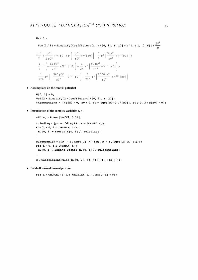
Hsvil =

Sum@1 i! * Simplify@Coefficient@i! * H@0, iD, r, iDD * r^i, 8 i, 0, 6<D +pr2

2

pr2

2+

pΘ2

2 r02+ V@r0D + r -

pΘ2

r03+ V¢@r0D +

1

2r2

3 pΘ2

r04+ V¢¢@r0D +

1

6r3 -

12 pΘ2

r05+ VH3L@r0D +

1

24r4

60 pΘ2

r06+ VH4L@r0D +

1

120r5 -

360 pΘ2

r07+ VH5L@r0D +

1

720r6

2520 pΘ2

r08+ VH6L@r0D

Assumptions on the central potential

H@0, 1D = 0;

Veff2 = Simplify@2 * Coefficient@H@0, 2D, r, 2DD;

$Assumptions = 8Veff2 > 0, r0 > 0, pΘ Sqrt@r0^3 V'@r0DD, pΘ > 0, 3 + g@r0D > 0<;

Introduction of the complex variables Ξ, Η

cfdiag = Power@Veff2, 1 4D;

rulediag = 8pr ® cfdiag PR, r ® R cfdiag<;

For@i = 0, i £ ORDMAX, i++,

HD@0, iD = Factor@H@0, iD . rulediagD;

Drulecomplex = 8PR ® 1 Sqrt@2D HΖ + I ΗL, R ® I Sqrt@2D HΖ - I ΗL<;

For@i = 0, i £ ORDMAX, i++,

HC@0, iD = Expand@Factor@HD@0, iD . rulecomplexDDDΩ = CoefficientRules@HC@0, 2D, 8Ζ, Η<D@@1DD@@2DD I;

Birkhoff normal form algorithm

For@i = ORDMAX + 1, i £ ORDBIRK, i++, HC@0, iD = 0D;


For@i = 3, i £ ORDBIRK, i++,

8ZHC@i - 2, iD, RHC@i - 2, iD< = myKernelRange@HC@i - 3, iDD;

C@iD = myHomologicalEquation@Ω, RHC@i - 2, iDD;

For@j = 0, j £ ORDBIRK, j++,

HC@i - 2, jD = Expand@Factor@HC@i - 3, jDDDD;

For@j = 0, j £ ORDBIRK, j++,

tmp = HC@i - 3, jD;

For@l = 1, l £ IntegerPart@HORDBIRK - jL Hi - 2LD, l++,

tmp = myPoissonBracket@tmp, C@iDD;

HC@i - 2, j + l Hi - 2LD += tmp;

HC@i - 2, j + l Hi - 2LD = Expand@Factor@HC@i - 2, j + l H i - 2LDDD;

tmp = Expand@Factor@tmp Hl + 1LDD;

DD

Dpteta = Sqrt@r0^3 V'@r0DD;

d1 = 1 D@pteta, r0D;

rulact = 8Ζ ® Sqrt@I1D, Η ® -I Sqrt@I1D<;

Haz@0D = HC@ORDBIRK - 2, 0D;

Haz@1D = HC@ORDBIRK - 2, 2D . rulact;



Ham = Haz@0D + Haz@1D + Haz@2D + Haz@3D;

F@r0_D := r0 V''@r0D V'@r0Dg0 = F@r0D;

g1 = D@F@r0D, 8r0, 1<D;

g2 = D@F@r0D, 8r0, 2<D;

g3 = D@F@r0D, 8r0, 3<D;

g4 = D@F@r0D, 8r0, 4<D;

We express the function V[r0] and its derivatives in terms of g and its derivatives

s0 = Flatten@Solve@g@r0D g0, D@V@r0D, 8r0, 2<DDD

:V¢¢@r0D ®g@r0D V¢@r0D

r0>

s1 = Flatten@Solve@D@g@r0D, 8r0, 1<D g1, D@V@r0D, 8r0, 3<DDD;

S1 = Flatten@Simplify@s1 . s0DD

:VH3L@r0D ®I-g@r0D + g@r0D2 + r0 g¢@r0DM V¢@r0D

r02>


s2 = Flatten@Solve@D@g@r0D, 8r0, 2<D g2, D@V@r0D, 8r0, 4<DDD;

S2 = Flatten@Simplify@s2 . s1 . s0DD

:VH4L@r0D ®1

r03

V¢@r0D I-3 g@r0D2 + g@r0D3 + g@r0D H2 + 3 r0 g¢@r0DL + r0 H-2 g¢@r0D + r0 g¢¢@r0DLM>s3 = Flatten@Solve@D@g@r0D, 8r0, 3<D g3, D@V@r0D, 8r0, 5<DDD;

S3 = Flatten@Simplify@s3 . s2 . s1 . s0DD

:VH5L@r0D ®1

r04V¢@r0D I-6 g@r0D3 + g@r0D4 +

g@r0D2 H11 + 6 r0 g¢@r0DL + 2 g@r0D I-3 - 7 r0 g¢@r0D + 2 r02 g¢¢@r0DM +

r0 I6 g¢@r0D + 3 r0 g¢@r0D2 + r0 I-3 g¢¢@r0D + r0 gH3L@r0DMMM>s4 = Flatten@Solve@D@g@r0D, 8r0, 4<D g4, D@V@r0D, 8r0, 6<DDD;

S4 = Flatten@Simplify@s4 . s3 . s2 . s1 . s0DD

:VH6L@r0D ®1

r05V¢@r0D I-10 g@r0D4 + g@r0D5 +

5 g@r0D3 H7 + 2 r0 g¢@r0DL + 10 g@r0D2 I-5 - 5 r0 g¢@r0D + r02 g¢¢@r0DM +

g@r0D I24 + 70 r0 g¢@r0D + 15 r02 g¢@r0D2 - 25 r02 g¢¢@r0D + 5 r03 gH3L@r0DM +

r0 I-20 r0 g¢@r0D2 + 2 g¢@r0D I-12 + 5 r02 g¢¢@r0DM +

r0 I12 g¢¢@r0D - 4 r0 gH3L@r0D + r02 gH4L@r0DMMM>d2 = Simplify@d1 . s0D;

We rewrite the Hamiltonian in BNF in terms of V¢@r0D, g[r0] and its derivatives

Hbirk = Factor@Expand@Ham . S4 . S3 . S2 . S1 . s0 . pΘ ® ptetaDD;

CoeffHbirk = CoefficientList@Hbirk, I1D;

Hbirk0 = Simplify@CoeffHbirk@@1DDD

V@r0D +1

2r0 V¢@r0D


H3 + g@r0DL V¢@r0Dr0


I-180 + 10 g@r0D3 - 2 g@r0D4 + 102 r0 g¢@r0D - 5 r02 g¢@r0D2 + g@r0D2 H94 - r0 g¢@r0DL +

9 r02 g¢¢@r0D + g@r0D I78 + 31 r0 g¢@r0D + 3 r02 g¢¢@r0DMM I48 r02 H3 + g@r0DL2M


Hbirk3 = Simplify@CoeffHbirk@@4DDD1

6912 r072 H3 + g@r0DL92 V¢@r0DI184 g@r0D7 + 20 g@r0D8 + 4044 r03 g¢@r0D3 - 235 r04 g¢@r0D4 +

4 g@r0D6 H279 + 17 r0 g¢@r0DL + g@r0D5 I4000 - 72 r0 g¢@r0D - 84 r02 g¢¢@r0DM +

54 r02 g¢@r0D2 I-494 + 25 r02 g¢¢@r0DM -

108 r0 g¢@r0D I-364 + 181 r02 g¢¢@r0D + 14 r03 gH3L@r0DM -

g@r0D4 I6820 + 3504 r0 g¢@r0D - 129 r02 g¢@r0D2 + 1152 r02 g¢¢@r0D + 48 r03 gH3L@r0DM +

27 I8880 + 3432 r02 g¢¢@r0D - 17 r04 g¢¢@r0D2 + 576 r03 gH3L@r0D + 24 r04 gH4L@r0DM -

g@r0D2 I1515 r02 g¢@r0D2 + 94 r03 g¢@r0D3 +

12 r0 g¢@r0D I-1389 + 100 r02 g¢¢@r0D + 14 r03 gH3L@r0DM + 3 I58 356 -

5976 r02 g¢¢@r0D + 17 r04 g¢¢@r0D2 - 1296 r03 gH3L@r0D - 72 r04 gH4L@r0DMM +

2 g@r0D3 I411 r02 g¢@r0D2 + r0 g¢@r0D I-3916 + 81 r02 g¢¢@r0DM +

12 I-3695 - 100 r02 g¢¢@r0D + 6 r03 gH3L@r0D + r04 gH4L@r0DMM +

2 g@r0D I533 r03 g¢@r0D3 + 9 r02 g¢@r0D2 I-964 + 25 r02 g¢¢@r0DM -

9 r0 g¢@r0D I-3408 + 643 r02 g¢¢@r0D + 56 r03 gH3L@r0DM +

9 I1416 + 4554 r02 g¢¢@r0D - 17 r04 g¢¢@r0D2 + 792 r03 gH3L@r0D + 36 r04 gH4L@r0DMMMHBIRK = Hbirk0 + Hbirk1 * I1 + Hbirk2 * I1^2 + Hbirk3 * I1^3;

The Burgers equation

The expansion of the two frequencies Ω1 and Ω2

$Assumptions = 8V'@r0D > 0, r0 > 0<;

The frequency Ω1

Ω1 = D@HBIRK, I1D;

CoeffΩ1 = CoefficientList@Ω1, I1D;

Ω10 = Simplify@CoeffΩ1@@1DDD

H3 + g@r0DL V¢@r0Dr0


I-180 + 10 g@r0D3 - 2 g@r0D4 + 102 r0 g¢@r0D - 5 r02 g¢@r0D2 + g@r0D2 H94 - r0 g¢@r0DL +

9 r02 g¢¢@r0D + g@r0D I78 + 31 r0 g¢@r0D + 3 r02 g¢¢@r0DMM I24 r02 H3 + g@r0DL2M


Ω12 = Simplify@CoeffΩ1@@3DDD1

2304 r072 H3 + g@r0DL92 V¢@r0DI184 g@r0D7 + 20 g@r0D8 + 4044 r03 g¢@r0D3 - 235 r04 g¢@r0D4 +

4 g@r0D6 H279 + 17 r0 g¢@r0DL + g@r0D5 I4000 - 72 r0 g¢@r0D - 84 r02 g¢¢@r0DM +

54 r02 g¢@r0D2 I-494 + 25 r02 g¢¢@r0DM -

108 r0 g¢@r0D I-364 + 181 r02 g¢¢@r0D + 14 r03 gH3L@r0DM -

g@r0D4 I6820 + 3504 r0 g¢@r0D - 129 r02 g¢@r0D2 + 1152 r02 g¢¢@r0D + 48 r03 gH3L@r0DM +

27 I8880 + 3432 r02 g¢¢@r0D - 17 r04 g¢¢@r0D2 + 576 r03 gH3L@r0D + 24 r04 gH4L@r0DM -

g@r0D2 I1515 r02 g¢@r0D2 + 94 r03 g¢@r0D3 +

12 r0 g¢@r0D I-1389 + 100 r02 g¢¢@r0D + 14 r03 gH3L@r0DM + 3 I58 356 -

5976 r02 g¢¢@r0D + 17 r04 g¢¢@r0D2 - 1296 r03 gH3L@r0D - 72 r04 gH4L@r0DMM +

2 g@r0D3 I411 r02 g¢@r0D2 + r0 g¢@r0D I-3916 + 81 r02 g¢¢@r0DM +

12 I-3695 - 100 r02 g¢¢@r0D + 6 r03 gH3L@r0D + r04 gH4L@r0DMM +

2 g@r0D I533 r03 g¢@r0D3 + 9 r02 g¢@r0D2 I-964 + 25 r02 g¢¢@r0DM -

9 r0 g¢@r0D I-3408 + 643 r02 g¢¢@r0D + 56 r03 gH3L@r0DM +

9 I1416 + 4554 r02 g¢¢@r0D - 17 r04 g¢¢@r0D2 + 792 r03 gH3L@r0D + 36 r04 gH4L@r0DMMMThe frequency Ω2

D2 = FullSimplify@d2D2

H3 + g@r0DL r0 V¢@r0DΩ2 = Simplify@D@HBIRK, r0D * D2 . s0D;

CoeffΩ2 = CoefficientList@Ω2, I1D;


V¢@r0Dr0

Ω21 = Simplify@CoeffΩ2@@2DDD-3 + 2 g@r0D + g@r0D2 + r0 g¢@r0D

r02 H3 + g@r0DL32

Ω22 = Simplify@CoeffΩ2@@3DDD1

24 r072 H3 + g@r0DL4 V¢@r0DI4 g@r0D5 - 111 r02 g¢@r0D2 + 10 r03 g¢@r0D3 - 4 g@r0D4 H2 + r0 g¢@r0DL -

g@r0D3 I248 + 13 r0 g¢@r0D + r02 g¢¢@r0DM + g¢@r0D I288 r0 - 39 r03 g¢¢@r0DM +

g@r0D2 I-720 + 62 r0 g¢@r0D + 28 r02 g¢¢@r0D + 3 r03 gH3L@r0DM +

9 I120 + 34 r02 g¢¢@r0D + 3 r03 gH3L@r0DM + g@r0D I-37 r02 g¢@r0D2 +

g¢@r0D I291 r0 - 13 r03 g¢¢@r0DM + 3 I-36 + 65 r02 g¢¢@r0D + 6 r03 gH3L@r0DMMMΩ23 = Simplify@CoeffΩ2@@4DDD;


The expansion of the ratio of the frequencies Ν=Ω1/Ω2

InvΩ20 = Simplify@1 Ω20D;

W1 = Simplify@Ω1 * InvΩ20D;

w20 = 1;

w21 = Simplify@Ω21 * InvΩ20D;

w21

-3 + 2 g@r0D + g@r0D2 + r0 g¢@r0DHr0 H3 + g@r0DLL32 V¢@r0D

w22 = Simplify@Ω22 * InvΩ20D;

w22

1

24 r03 H3 + g@r0DL4 V¢@r0DI4 g@r0D5 - 111 r02 g¢@r0D2 + 10 r03 g¢@r0D3 - 4 g@r0D4 H2 + r0 g¢@r0DL -

g@r0D3 I248 + 13 r0 g¢@r0D + r02 g¢¢@r0DM + g¢@r0D I288 r0 - 39 r03 g¢¢@r0DM +

g@r0D2 I-720 + 62 r0 g¢@r0D + 28 r02 g¢¢@r0D + 3 r03 gH3L@r0DM +

9 I120 + 34 r02 g¢¢@r0D + 3 r03 gH3L@r0DM + g@r0D I-37 r02 g¢@r0D2 +

g¢@r0D I291 r0 - 13 r03 g¢¢@r0DM + 3 I-36 + 65 r02 g¢¢@r0D + 6 r03 gH3L@r0DMMMw23 = Simplify@Ω23 * InvΩ20D;

Omega2 = SimplifyAw20 + w21 * I11+ w22 * I12

+ w23 * I13E;

W2 = Series@1 Omega2, 8I1, 0, 3<D;

Ν = Simplify@W1 * W2D;

The Burgers equation

ΝSecon = Simplify@Ν * D@Ν, r0D * D2D;

ΝPrim = Simplify@D@Ν, I1DD;

Burg = ΝPrim - ΝSecon;

We extract the order 0 (burg0) and the order 1 (burg1) of the Burgers equation

CoeffBurg = CoefficientList@Burg, I1D;

burg0 = Simplify@Expand@CoeffBurg@@1DDDD

-I14 g@r0D3 + 2 g@r0D4 + 42 r0 g¢@r0D + 5 r02 g¢@r0D2 + g@r0D2 H26 + r0 g¢@r0DL +

g@r0D I-6 + 17 r0 g¢@r0D - 3 r02 g¢¢@r0DM - 9 I4 + r02 g¢¢@r0DMM J24 r032 H3 + g@r0DL2 V¢@r0D N


burg1 = Simplify@CoeffBurg@@2DDD . s0

1

1152 r03 H3 + g@r0DL92 V¢@r0D2I-48 g@r0D H3 + g@r0DL2 V¢@r0D

I14 g@r0D3 + 2 g@r0D4 - 30 r0 g¢@r0D + 5 r02 g¢@r0D2 + g@r0D2 H26 + r0 g¢@r0DL -

9 I4 + r02 g¢¢@r0DM - g@r0D I6 + 7 r0 g¢@r0D + 3 r02 g¢¢@r0DMM +

V¢@r0D I376 g@r0D7 + 20 g@r0D8 + 444 r03 g¢@r0D3 - 235 r04 g¢@r0D4 +

4 g@r0D6 H687 + 17 r0 g¢@r0DL + g@r0D5 I9664 + 1080 r0 g¢@r0D - 84 r02 g¢¢@r0DM +

54 r02 g¢@r0D2 I26 + 25 r02 g¢¢@r0DM + g@r0D4

I15 068 + 6336 r0 g¢@r0D + 129 r02 g¢@r0D2 - 1248 r02 g¢¢@r0D - 48 r03 gH3L@r0DM -

108 r0 g¢@r0D I44 + 9 r02 g¢¢@r0D + 14 r03 gH3L@r0DM -

27 I-240 + 648 r02 g¢¢@r0D + 17 r04 g¢¢@r0D2 - 24 r04 gH4L@r0DM -

g@r0D2 I-5349 r02 g¢@r0D2 + 94 r03 g¢@r0D3 +

12 r0 g¢@r0D I-1569 - 72 r02 g¢¢@r0D + 14 r03 gH3L@r0DM + 3 I7380 +

7128 r02 g¢¢@r0D + 17 r04 g¢¢@r0D2 + 432 r03 gH3L@r0D - 72 r04 gH4L@r0DMM +

2 g@r0D I-67 r03 g¢@r0D3 + 9 r02 g¢@r0D2 I388 + 25 r02 g¢¢@r0DM -

9 r0 g¢@r0D I-168 - 45 r02 g¢¢@r0D + 56 r03 gH3L@r0DM -

9 I744 + 1710 r02 g¢¢@r0D + 17 r04 g¢¢@r0D2 + 72 r03 gH3L@r0D - 36 r04 gH4L@r0DMM +

2 g@r0D3 I723 r02 g¢@r0D2 + r0 g¢@r0D I8444 + 81 r02 g¢¢@r0DM +

12 I49 - 306 r02 g¢¢@r0D - 18 r03 gH3L@r0D + r04 gH4L@r0DMMMM The iterative procedure

We put burg0 and burg1 equal to 0 and solve with respect to g¢¢@r0D and gH4L@r0D respectively

equa1 = Flatten@Simplify@Solve@burg0 0, D@g@r0D, 8r0, 2<DDDD

9g¢¢@r0D ® I-36 + 14 g@r0D3 + 2 g@r0D4 + 42 r0 g¢@r0D + 5 r02 g¢@r0D2 +

g@r0D2 H26 + r0 g¢@r0DL + g@r0D H-6 + 17 r0 g¢@r0DLM I3 r02 H3 + g@r0DLM=equazione2 = Simplify@equa1@@1DD@@2DDD

I-36 + 14 g@r0D3 + 2 g@r0D4 + 42 r0 g¢@r0D + 5 r02 g¢@r0D2 +

g@r0D2 H26 + r0 g¢@r0DL + g@r0D H-6 + 17 r0 g¢@r0DLM I3 r02 H3 + g@r0DLM


equa2 = Flatten@Simplify@Solve@burg1 0, D@g@r0D, 8r0, 4<DDDD

:gH4L@r0D ®

1

24 r04 H3 + g@r0DL3I-280 g@r0D7 - 20 g@r0D8 - 444 r03 g¢@r0D3 + 235 r04 g¢@r0D4 -

4 g@r0D6 H375 + 17 r0 g¢@r0DL + 4 g@r0D5 I-880 - 258 r0 g¢@r0D + 21 r02 g¢¢@r0DM -

54 r02 g¢@r0D2 I26 + 25 r02 g¢¢@r0DM + 27 I-240 + 648 r02 g¢¢@r0D + 17 r04 g¢¢@r0D2M +

108 r0 g¢@r0D I44 + 9 r02 g¢¢@r0D + 14 r03 gH3L@r0DM + g@r0D4

I-1820 - 6384 r0 g¢@r0D - 129 r02 g¢@r0D2 + 1104 r02 g¢¢@r0D + 48 r03 gH3L@r0DM -

2 g@r0D3 I603 r02 g¢@r0D2 + r0 g¢@r0D I9956 + 81 r02 g¢¢@r0DM -

12 I275 + 252 r02 g¢¢@r0D + 18 r03 gH3L@r0DMM -



9 I-120 + 1494 r02 g¢¢@r0D + 17 r04 g¢¢@r0D2 + 72 r03 gH3L@r0DMM +

g@r0D2 I-3909 r02 g¢@r0D2 + 94 r03 g¢@r0D3 +

12 r0 g¢@r0D I-2541 - 72 r02 g¢¢@r0D + 14 r03 gH3L@r0DM +

3 I3060 + 5832 r02 g¢¢@r0D + 17 r04 g¢¢@r0D2 + 432 r03 gH3L@r0DMMM>equazione4 = Simplify@equa2@@1DD@@2DDD

1

24 r04 H3 + g@r0DL3I-280 g@r0D7 - 20 g@r0D8 - 444 r03 g¢@r0D3 + 235 r04 g¢@r0D4 -

4 g@r0D6 H375 + 17 r0 g¢@r0DL + 4 g@r0D5 I-880 - 258 r0 g¢@r0D + 21 r02 g¢¢@r0DM -

54 r02 g¢@r0D2 I26 + 25 r02 g¢¢@r0DM + 27 I-240 + 648 r02 g¢¢@r0D + 17 r04 g¢¢@r0D2M +

108 r0 g¢@r0D I44 + 9 r02 g¢¢@r0D + 14 r03 gH3L@r0DM +

g@r0D4 I-1820 - 6384 r0 g¢@r0D - 129 r02 g¢@r0D2 + 1104 r02 g¢¢@r0D + 48 r03 gH3L@r0DM -

2 g@r0D3 I603 r02 g¢@r0D2 + r0 g¢@r0D I9956 + 81 r02 g¢¢@r0DM -

12 I275 + 252 r02 g¢¢@r0D + 18 r03 gH3L@r0DMM -



9 I-120 + 1494 r02 g¢¢@r0D + 17 r04 g¢¢@r0D2 + 72 r03 gH3L@r0DMM +

g@r0D2 I-3909 r02 g¢@r0D2 + 94 r03 g¢@r0D3 +

12 r0 g¢@r0D I-2541 - 72 r02 g¢¢@r0D + 14 r03 gH3L@r0DM +

3 I3060 + 5832 r02 g¢¢@r0D + 17 r04 g¢¢@r0D2 + 432 r03 gH3L@r0DMMMWe insert g¢¢@r0D in equazione4


equazione4new = Simplify@equazione4 . equa1D1

9 r04 H3 + g@r0DL3I-25 920 + 374 g@r0D7 + 22 g@r0D8 + 9828 r02 g¢@r0D2 - 1434 r03 g¢@r0D3 -

140 r04 g¢@r0D4 + g@r0D6 H2712 - 47 r0 g¢@r0DL - 4 g@r0D5 H-2687 + 69 r0 g¢@r0DL +

2 g@r0D4 I12 083 + 333 r0 g¢@r0D - 42 r02 g¢@r0D2 + 9 r03 gH3L@r0DM +

27 r0 g¢@r0D I908 + 21 r03 gH3L@r0DM +

g@r0D3 I26 238 + 9116 r0 g¢@r0D - 729 r02 g¢@r0D2 + 162 r03 gH3L@r0DM +

g@r0D I4527 r02 g¢@r0D2 - 781 r03 g¢@r0D3 + 54 r0 g¢@r0D I760 + 7 r03 gH3L@r0DM +

54 I-664 + 9 r03 gH3L@r0DMM + g@r0D2 I-1014 r02 g¢@r0D2 - 101 r03 g¢@r0D3 +

63 r0 g¢@r0D I455 + r03 gH3L@r0DM + 54 I-46 + 9 r03 gH3L@r0DMMMWe compute the second order derivative of equazione2 , we solve for gH4L@r0D and we equal this new expression to

equazione4new. We solve for gH3L@r0Dequazione2Der2 = Simplify@D@equazione2, 8r0, 2<DD

1

3 r04 H3 + g@r0DL3I12 g@r0D6 + 10 r04 g¢@r0D4 +

6 g@r0D5 I26 - 4 r0 g¢@r0D + r02 g¢¢@r0DM + g¢@r0D2 I378 r02 - 75 r04 g¢¢@r0DM +

g@r0D4 I768 - 278 r0 g¢@r0D + 12 r02 g¢@r0D2 + 68 r02 g¢¢@r0D + r03 gH3L@r0DM +

9 r0 g¢@r0D I60 + 9 r02 g¢¢@r0D + 10 r03 gH3L@r0DM +

18 I-108 - 39 r02 g¢¢@r0D + 5 r04 g¢¢@r0D2 + 21 r03 gH3L@r0DM + g@r0D3 I122 r02 g¢@r0D2 +

262 r02 g¢¢@r0D + r0 g¢@r0D I-1186 + 3 r02 g¢¢@r0DM + 23 I72 + r03 gH3L@r0DMM +

g@r0D2 I972 + 450 r02 g¢@r0D2 + 306 r02 g¢¢@r0D + 10 r04 g¢¢@r0D2 +

153 r03 gH3L@r0D + r0 g¢@r0D I-2142 + 27 r02 g¢¢@r0D + 10 r03 gH3L@r0DMM +

g@r0D I-324 r02 g¢¢@r0D + 60 r04 g¢¢@r0D2 + g¢@r0D2 I702 r02 - 25 r04 g¢¢@r0DM +

405 I-4 + r03 gH3L@r0DM + 3 r0 g¢@r0D I-378 + 27 r02 g¢¢@r0D + 20 r03 gH3L@r0DMMMequa3 = Flatten@Simplify@

Solve@equazione2Der2 - equazione4new 0, D@g@r0D, 8r0, 3<DD . equa1DD9gH3L@r0D ® I98 496 - 10 g@r0D7 + 10 g@r0D8 - 131 328 r0 g¢@r0D - 9450 r02 g¢@r0D2 +

5757 r03 g¢@r0D3 + 385 r04 g¢@r0D4 + g@r0D6 H-1788 + 217 r0 g¢@r0DL + 2 g@r0D5H-7742 + 1131 r0 g¢@r0DL + g@r0D4 I-57 422 + 7254 r0 g¢@r0D + 519 r02 g¢@r0D2M +

g@r0D3 I-96 594 - 3136 r0 g¢@r0D + 4932 r02 g¢@r0D2M +

g@r0D2 I-31 968 - 72 855 r0 g¢@r0D + 14 529 r02 g¢@r0D2 + 373 r03 g¢@r0D3M +

2 g@r0D I52 380 - 84 375 r0 g¢@r0D + 5031 r02 g¢@r0D2 + 1519 r03 g¢@r0D3MM I9 r03 H3 + g@r0DL2 I-42 + g@r0D + 5 g@r0D2 + 11 r0 g¢@r0DMM=


equazione3 = Simplify@equa3@@1DD@@2DDD

I98 496 - 10 g@r0D7 + 10 g@r0D8 - 131 328 r0 g¢@r0D - 9450 r02 g¢@r0D2 + 5757 r03 g¢@r0D3 +

385 r04 g¢@r0D4 + g@r0D6 H-1788 + 217 r0 g¢@r0DL + 2 g@r0D5 H-7742 + 1131 r0 g¢@r0DL +

g@r0D4 I-57 422 + 7254 r0 g¢@r0D + 519 r02 g¢@r0D2M +

g@r0D3 I-96 594 - 3136 r0 g¢@r0D + 4932 r02 g¢@r0D2M +

g@r0D2 I-31 968 - 72 855 r0 g¢@r0D + 14 529 r02 g¢@r0D2 + 373 r03 g¢@r0D3M +

2 g@r0D I52 380 - 84 375 r0 g¢@r0D + 5031 r02 g¢@r0D2 + 1519 r03 g¢@r0D3MM I9 r03 H3 + g@r0DL2 I-42 + g@r0D + 5 g@r0D2 + 11 r0 g¢@r0DMMWe compute the first order derivative of the equazione2 and we solve for gH3L@r0D

equazione2Der1 = Simplify@D@equazione2, 8r0, 1<D . equa1D1

9 r03 H3 + g@r0DL2I-864 + 36 g@r0D5 + 2 g@r0D6 + 1080 r0 g¢@r0D + 657 r02 g¢@r0D2 + 35 r03 g¢@r0D3 +

3 g@r0D4 H76 + 13 r0 g¢@r0DL + g@r0D3 H616 + 327 r0 g¢@r0DL +

3 g@r0D2 I174 + 343 r0 g¢@r0D + 6 r02 g¢@r0D2M +

3 g@r0D I-180 + 519 r0 g¢@r0D + 91 r02 g¢@r0D2MMWe equal the two expressions for gH3L@r0D obtaining two equations for g¢@r0D

Eq1 = Simplify@equazione2Der1 - equazione3D;

equa1New = Simplify@Solve@Eq1 0, D@g@r0D, 8r0, 1<DDD

99g¢@r0D ® I177 + 110 g@r0D + 5 g@r0D2 - 4 g@r0D3 +

3 ,IH3 + g@r0DL2 I851 + 690 g@r0D + 171 g@r0D2 + 16 g@r0D3MMM H29 r0 - 2 r0 g@r0DL=, 9g¢@r0D ® I177 + 110 g@r0D + 5 g@r0D2 - 4 g@r0D3 -

3 ,IH3 + g@r0DL2 I851 + 690 g@r0D + 171 g@r0D2 + 16 g@r0D3MMM H29 r0 -

2 r0 g@r0DL==equazione11 = equa1New@@1DD@@1DD@@2DD

K177 + 110 g@r0D + 5 g@r0D2 - 4 g@r0D3 +

3 H3 + g@r0DL2 I851 + 690 g@r0D + 171 g@r0D2 + 16 g@r0D3M O H29 r0 - 2 r0 g@r0DLequazione12 = Simplify@equa1New@@2DD@@1DD@@2DDD

K177 + 110 g@r0D + 5 g@r0D2 - 4 g@r0D3 -

3 H3 + g@r0DL2 I851 + 690 g@r0D + 171 g@r0D2 + 16 g@r0D3M O H29 r0 - 2 r0 g@r0DLWe consider the first one, compute the first oder derivative, susbtitute the expression for g¢@r0D and solve for g¢¢@r0D

equa1New@@1DD@@1DD@@2DD

K177 + 110 g@r0D + 5 g@r0D2 - 4 g@r0D3 +

3 H3 + g@r0DL2 I851 + 690 g@r0D + 171 g@r0D2 + 16 g@r0D3M O H29 r0 - 2 r0 g@r0DL


Eq1Der = Simplify@D@equazione11, 8r0, 1<D . equa1New@@1DD@@1DDD

-II177 + 110 g@r0D + 5 g@r0D2 - 4 g@r0D3 +

3 ,IH3 + g@r0DL2 I851 + 690 g@r0D + 171 g@r0D2 + 16 g@r0D3MMMI179 400 3 + 200 686 3 g@r0D + 626 3 g@r0D4 - 48 3 g@r0D5 +

2703 ,IH3 + g@r0DL2 I851 + 690 g@r0D + 171 g@r0D2 + 16 g@r0D3MM +

406 g@r0D ,IH3 + g@r0DL2 I851 + 690 g@r0D + 171 g@r0D2 + 16 g@r0D3MM +

2 g@r0D2 I40 455 3 -

181 ,IH3 + g@r0DL2 I851 + 690 g@r0D + 171 g@r0D2 + 16 g@r0D3MMM + 2 g@r0D3

I6813 3 + 8 ,IH3 + g@r0DL2 I851 + 690 g@r0D + 171 g@r0D2 + 16 g@r0D3MMMMM Kr02 H-29 + 2 g@r0DL3 H3 + g@r0DL2 I851 + 690 g@r0D + 171 g@r0D2 + 16 g@r0D3M O

equazione2New = Simplify@equazione2 . equa1New@@1DDD1

r02 H29 - 2 g@r0DL2K50 760 - 249 g@r0D3 - 138 g@r0D4 + 32 g@r0D5 +

332 3 H3 + g@r0DL2 I851 + 690 g@r0D + 171 g@r0D2 + 16 g@r0D3M -

2 g@r0D2 I-5594 + 7 3 ,IH3 + g@r0DL2 I851 + 690 g@r0D + 171 g@r0D2 + 16 g@r0D3MMM +

3 g@r0D I15 469 + 19 3 ,IH3 + g@r0DL2 I851 + 690 g@r0D + 171 g@r0D2 + 16 g@r0D3MMMOWe equal the two expressions for g¢¢@r0Dand obtain that the solutions are g@r0D = constant. Precisely,

Num = Numerator@Simplify@Eq1Der - equazione2NewDD;

Soluzioni1 = Flatten@Simplify@Solve@Num 0DDD

:g@r0D ® -3, g@r0D ®29

2, g@r0D ® RootA

179 147 + 458 229 ð1 + 394 875 ð12 + 162 491 ð13 + 35 862 ð14 + 4140 ð15 + 200 ð16 &, 1E,

g@r0D ® RootA179 147 + 458 229 ð1 + 394 875 ð12 + 162 491 ð13 +

35 862 ð14 + 4140 ð15 + 200 ð16 &, 5E, g@r0D ® RootA179 147 + 458 229 ð1 + 394 875 ð12 + 162 491 ð13 + 35 862 ð14 + 4140 ð15 + 200 ð16 &, 6E>

NSolve@Num 0D88g@r0D ® -3.85584 + 2.12369 ä<, 8g@r0D ® -3.85584 - 2.12369 ä<,8g@r0D ® -3.<, 8g@r0D ® -3.<, 8g@r0D ® -3.<, 8g@r0D ® -2.14151<<88g@r0D ® -3.85584 + 2.12369 ä<, 8g@r0D ® -3.85584 - 2.12369 ä<,8g@r0D ® -3.<, 8g@r0D ® -3.<, 8g@r0D ® -3.<, 8g@r0D ® -2.14151<<

Analogously, we consider the second equation for g¢@r0D and we do the same

Eq2Der = Simplify@D@equazione12, 8r0, 1<D . equa1New@@2DDD;

equazione2New2 = Simplify@equazione2 . equa1New@@2DDD;

Num2 = Numerator@Simplify@Eq2Der - equazione2New2DD;


Soluzioni2 = Flatten@Simplify@Solve@Num2 0DDD9g@r0D ® -3, g@r0D ® -2, g@r0D ® 1, g@r0D ® RootA

179 147 + 458 229 ð1 + 394 875 ð12 + 162 491 ð13 + 35 862 ð14 + 4140 ð15 + 200 ð16 &, 2E,

g@r0D ® RootA179 147 + 458 229 ð1 + 394 875 ð12 + 162 491 ð13 +

35 862 ð14 + 4140 ð15 + 200 ð16 &, 3E, g@r0D ® RootA179 147 + 458 229 ð1 + 394 875 ð12 + 162 491 ð13 + 35 862 ð14 + 4140 ð15 + 200 ð16 &, 4E=

NSolve@Num2 0D88g@r0D ® -3.<, 8g@r0D ® -3.<, 8g@r0D ® -3.<,8g@r0D ® -2.<, 8g@r0D ® 1.<, 8g@r0D ® -0.743563<< Check of the solutions

eq = Numerator@equazione2 . g'@r0D ® 0D

-36 - 6 g@r0D + 26 g@r0D2 + 14 g@r0D3 + 2 g@r0D4

Check for the first group of solutions

For@i = 1, i £ 5, i++,

Solut1@iD = FullSimplify@eq . Soluzioni1@@iDDDD;

For@i = 1, i £ 5, i++,

If@Simplify@Solut1@iD 0D,

Print@"g@r0D=", Soluzioni1@@iDD@@2DD, " is a solution" D,

Print@"g@r0D=", Soluzioni1@@iDD@@2DD, " is not a solution" DDD

g@r0D=-3 is a solution

g@r0D=29

2is not a solution

g@r0D=

RootA179 147 + 458 229 ð1 + 394 875 ð12 + 162 491 ð13 + 35 862 ð14 + 4140 ð15 + 200 ð16 &, 1Eis not a solution

g@r0D=


g@r0D=


Check for the second group of solutions

For@i = 1, i £ 6, i++,

Solut2@iD = FullSimplify@eq . Soluzioni2@@iDDDD;


For@i = 1, i £ 6, i++,

If@Simplify@Solut2@iD 0D,

Print@"g@r0D=", Soluzioni2@@iDD@@2DD, " is a solution" D,

Print@"g@r0D=", Soluzioni2@@iDD@@2DD, " is not a solution" DDD



g@r0D=1 is a solution

g@r0D=


g@r0D=


g@r0D=


We obtain that g[r0]=-3, g[r0]=-2 and g[r0]=1 are solutions. We exclude the case g[r0]=-3 since it does not satisfy thehypothesis on the effective potential


Bibliography

[Arn91] Vladimir I Arnold. Mathematical methods of classical mechanics. trans-lated from the 1974 russian original by k. vogtmann and a. weinstein.corrected reprint of the second (1989) edition. Graduate Texts in Math-ematics, 60:229234, 1991.

[Bam99] Dario Bambusi. Nekhoroshev theorem for small amplitude solutions innonlinear schrödinger equations. Mathematische Zeitschrift, 230(2):345387, 1999.

[BC17] L. Biasco and L. Chierchia. KAM Theory for secondary tori. ArXive-prints, February 2017.

[Ber73] J. Bertrand. Théorèm relatif au mouvement d'un point attiré vers uncentre xe. Comptes Rendus, 77:849853, 1873.

[BF17] Dario Bambusi and Alessandra Fusè. Nekhoroshev theorem for perturb-ations of the central motion. Regul. Chaotic Dyn., 22(1):1826, 2017.

[BFS17] D. Bambusi, A. Fusè, and M. Sansottera. Quasi-convexity of theHamiltonian for non Harmonic or non Keplerian central potentials.ArXiv e-prints, May 2017.

[Bla01] A. D. Blaom. A geometric setting for Hamiltonian perturbation theory.Number 727. American Mathematical Soc., 2001.

[Ehr48] Charles Ehresmann. Les connexions innitésimales dans un espace brédiérentiable. Séminaire Bourbaki, 1:153168, 1948.

[Fas95] F. Fassò. Hamiltonian perturbation theory on a manifold. CelestialMechanics and Dynamical Astronomy, 62(1):4369, 1995.

[Fas05] F. Fassò. Superintegrable Hamiltonian systems: geometry and perturb-ations. Acta Applicandae Mathematica, 87(1-3):93121, 2005.

106

BIBLIOGRAPHY 107

[FK04] J. Féjoz and L. Kaczmarek. Sur le théorème de Bertrand (d'après MichaelHerman). Ergodic Theory and Dynamical Systems, 24(05):15831589,2004.

[GCB16] M. Guzzo, L. Chierchia, and G. Benettin. The steep Nekhoroshev'stheorem. Comm. Math. Phys., 342(2):569601, 2016.

[Gio01] A. Giorgilli. Unstable equilibria of Hamiltonian systems. Discrete Con-tin. Dynam. Systems, 7(4):855871, 2001.

[GM96] Massimilliano Guzzo and Alessandro Morbidelli. Construction of a nek-horoshev like result for the asteroid belt dynamical system. CelestialMechanics and Dynamical Astronomy, 66(3):255292, 1996.

[Guz99] Massimiliano Guzzo. Nekhoroshev stability of quasi-integrable degen-erate hamiltonian systems. Regular and chaotic dynamics, 4(2):78102,1999.

[KM12] Mihail Vladimirovi Karasev and Viktor Pavlovi Maslov. Nonlinear Pois-son brackets: geometry and quantization, volume 119. American Math-ematical Soc., 2012.

[Loc92] Pierre Lochak. Canonical perturbation theory: an approach based onjoint approximations. Uspekhi Mat. Nauk, 47(6):288, 1992.

[MF78] A.S. Mishchenko and A.T. Fomenko. Generalized liouville method ofintegration of hamiltonian systems. Functional analysis and its applica-tions, 12(2):113121, 1978.

[Nei87] AI Neishtadt. On the change in the adiabatic invariant on crossing aseparatrix in systems with two degrees of freedom. Journal of AppliedMathematics and Mechanics, 51(5):586592, 1987.

[Nek72] N.N. Nekhoroshev. Action-angle variables, and their generalizations.Trudy Moskovskogo Matematicheskogo Obshchestva, 26:181198, 1972.

[Nek77] Nikolai Nikolaevich Nekhoroshev. An exponential estimate of the timeof stability of nearly integrable Hamiltonian systems. Uspehi Mat. Nauk,32(6(198)):566, 287, 1977.

[Nek79] Nikolai Nikolaevich Nekhoroshev. An exponential estimate of the timeof stability of nearly integrable Hamiltonian systems. II. Trudy Sem.Petrovsk., (5):550, 1979.

BIBLIOGRAPHY 108

[Nie96] Laurent Niederman. Stability over exponentially long times in the plan-etary problem. Nonlinearity, 9(6):1703, 1996.

[Sch96] Wolfgang M Schmidt. Diophantine approximation, volume 785. SpringerScience & Business Media, 1996.